Article

A Measure–Correlate–Predict Approach for Transferring Wind Speeds from MERRA2 Reanalysis to Wind Turbine Hub Heights

1
Department of Mechanical Engineering, University of Las Palmas de Gran Canaria, Campus de Tafira s/n, 35017 Las Palmas de Gran Canaria, Spain
2
Department of Sustainability and Planning, Aalborg University, Rendsburggade 14, 9000 Aalborg, Denmark
*
Author to whom correspondence should be addressed.
J. Mar. Sci. Eng. 2025, 13(7), 1213; https://doi.org/10.3390/jmse13071213
Submission received: 28 May 2025 / Revised: 12 June 2025 / Accepted: 18 June 2025 / Published: 23 June 2025
(This article belongs to the Section Coastal Engineering)

Abstract

Reanalysis datasets, such as MERRA2, are frequently used in wind resource assessments. However, their wind speed data are typically limited to fixed altitudes that differ from wind turbine hub heights, which introduces significant uncertainty in energy yield estimations. To address this challenge, we propose a reproducible Measure–Correlate–Predict (MCP) framework that integrates Random Forest (RF) supervised learning to estimate hub-height wind speeds from MERRA2 data at 50 m. The method includes the fitting of 21 vertical wind profile models using data at 2 m, 10 m, and 50 m, with model selection based on the minimum mean square error. The approach was applied to seven wind-prone locations in the Canary Islands, selected for their strategic relevance in current or planned wind energy development. Results indicate that a three-parameter logarithmic wind profile achieved the best fit in 51.31% of cases, significantly outperforming traditional single-parameter models. The RF-based MCP predictions at different hub heights achieved RMSE metrics below 0.425 m/s across a 10-year period. These findings demonstrate the potential of combining physical modeling with machine learning to enhance wind speed extrapolation from reanalysis data and support informed wind energy planning in data-scarce regions.

1. Introduction

Renewable energy resources are integral to sustainable energy planning, significantly contributing to the mitigation of climate change, the reduction of fossil fuel dependency, and enhancing local economic development and living conditions [1]. Effective modeling of these resources supports optimal planning, efficient management, and strategic deployment of renewable energy technologies, especially in isolated or islanded energy systems where resource management is critical [2]. This type of modeling also enables extensive analysis of future scenarios, aiding decision-makers in evaluating the feasibility of renewable integration and ensuring reliable energy system operation and planning [3].
The power produced by a wind turbine (WT) at any given moment is directly proportional to the air density and the cube of the wind speed at hub height [4]. Among these variables, wind speed has the greatest influence on both the estimation of wind power density (WPD) [5] and the energy output of the WT [6]. In fact, many studies assume air density to be constant over time, typically adopting a value of 1.225 kg m−3, which corresponds to standard atmospheric conditions [7], or using its mean value estimated at hub height [8]. Accurately estimating hub-height wind speeds is critical for wind farm operation and planning, as highlighted by Yu and Vautard [9] and Crippa et al. [10]. Furthermore, precise knowledge of wind speed profiles is essential for assessing wind farm feasibility, as emphasized by Mohandes et al. [11].
When no historical wind speed measurements are available at a target site (TS) to evaluate daily, seasonal, or interannual variability, statistical methods known as Measure–Correlate–Predict (MCP) techniques are commonly used [12]. These methods require historical wind speed data from nearby reference stations. However, when MCP methods are infeasible for long-term wind speed estimation at a TS, reanalysis data provide an alternative solution [12]. According to de Aquino et al. [13], reanalysis datasets have gained increasing importance in recent years as a promising alternative for climate studies in regions with sparse or missing meteorological data. One of the most widely used datasets is the Modern-Era Retrospective Analysis for Research and Applications (MERRA2) [14], which is publicly available and provides extensive historical records. Produced by NASA’s Global Modelling and Assimilation Office (GMAO), MERRA2 offers hourly wind speed data at three heights above ground level (2 m, 10 m, and 50 m). This dataset is widely used in renewable energy resource modeling [7]. However, when wind speeds at heights other than those provided by MERRA2 are required, appropriate vertical wind profile models must be employed to account for wind variability with height while ensuring a good fit to the reanalysis data. For this purpose, practitioners use available models listed in the literature (see Section 1.1).

1.1. Literature Review of Reanalysis Wind Speed Transfer Models

According to Pelser et al. [15], in 2021 the average hub height of onshore wind turbines in the United States was approximately 94 m. However, in Europe, the average hub height for turbines installed in 2020 was 104 m. Additionally, the authors noted that wind speed data are typically provided at heights between 10 and 50 m above ground level.
Various models have been proposed in the literature to extrapolate wind speed from a reference height to WT hub height. Among the most used are the logarithmic law and the power law models [13,15,16,17,18,19,20]. According to the analysis made by Pelser et al. [15], forty studies employed the logarithmic law, while another forty-four utilized the power law. Likewise, the authors [15] found that five studies used linear spline interpolation to determine wind speed at hub height based on two known wind speeds, whereas one hundred and three studies did not specify the method used for extrapolation.
The log law model, derived from meteorological theory, is typically applied under the assumption that the boundary layer is neutrally buoyant [16]. According to Watson [19], this is a common approximation when stability information is unavailable, in which case the logarithmic profile is considered adiabatic. Conversely, the power law model is empirical and is primarily used in engineering and mathematical applications rather than being grounded in meteorological theory [17]. For both the logarithmic and power law models, if wind speed data are available at two different heights, model parameters can be estimated accordingly. According to Gualtieri [21], the power law is the most widely used method in the literature, likely due to its relative reliability and ease of use. However, interpolation between two heights may be required as the preferred method. Gruber et al. [22] applied the power law by estimating the shear exponent factor from MERRA2 wind speeds recorded at 10 m and 50 m. Several studies have proposed logarithmic wind profile models for MERRA2 data in different regions, including Australia [23], the Arabian Peninsula [24], the USA [25], South Germany [26], and mainland China [27,28,29]. In these studies, the zero-plane displacement was incorporated under the assumption of neutral atmospheric stratification. Other approaches have considered more complex three-parameter logarithmic wind profile models [30]. These models introduce additional parameters such as the Monin–Obukhov length (which depends on boundary layer stability) and a term related to friction velocity and the von Kármán constant. The unknown parameters are determined by solving a three-dimensional equation system using MERRA2 wind speed data at 2 m, 10 m, and 50 m.
Recently, alternative methods based on machine learning (ML) have been explored, including a set of limitations which are discussed below. Yu and Vautard [9] proposed a transfer method that employs ML techniques to estimate ERA5 wind speeds at 100 m based on wind speeds at 10 m. The authors reported that ML algorithms provided more accurate estimations at 100 m than traditional extrapolation models. However, this approach requires known wind speed data at hub height for supervised learning and does not generalize to other heights. Similarly, Valsaraj et al. [31] introduced a symbolic regression method for wind speed extrapolation. However, their approach also requires wind speed measurements at multiple heights, including hub height, making it impractical when only MERRA2 data are available. Mohandes et al. [11] proposed an adaptive neuro-fuzzy inference system to address these limitations. Their approach estimates wind speeds iteratively based on four equally spaced height measurements (10 m, 20 m, 30 m, and 40 m). Subsequent works by Mohandes and Rehman [32], Nuha et al. [33], Islam et al. [34], Al-Shaikhi et al. [35,36], and Rheman et al. [37] have extended this concept using different ML techniques. However, these methods are not directly applicable to MERRA2 data given the irregular spacing of the available height levels (2 m, 10 m, and 50 m) and their limited number.

1.2. Aim, Novelty, and Key Contributions of This Paper

To overcome the limitations discussed in Section 1.1, this study develops a methodology to estimate hourly wind speeds at hub height which combines physical extrapolation models and ML techniques. The approach integrates an MCP strategy with Random Forest (RF) regression, trained using one year of hub-height data. A total of 21 vertical wind profile models are evaluated based on their fit to MERRA2 wind speed observations at 2 m, 10 m, and 50 m. For each hour, the model that minimizes the mean square error (MSE) is selected to provide the input for the RF training phase. This combined strategy addresses a key gap in the existing literature by enabling robust, data-driven extrapolation without relying on dense vertical measurements.
The considered wind profiles include the following:
  • Engineering-based and mathematical models, such as the power law and log law.
  • Meteorologically derived formulations, including three-parameter log profiles.
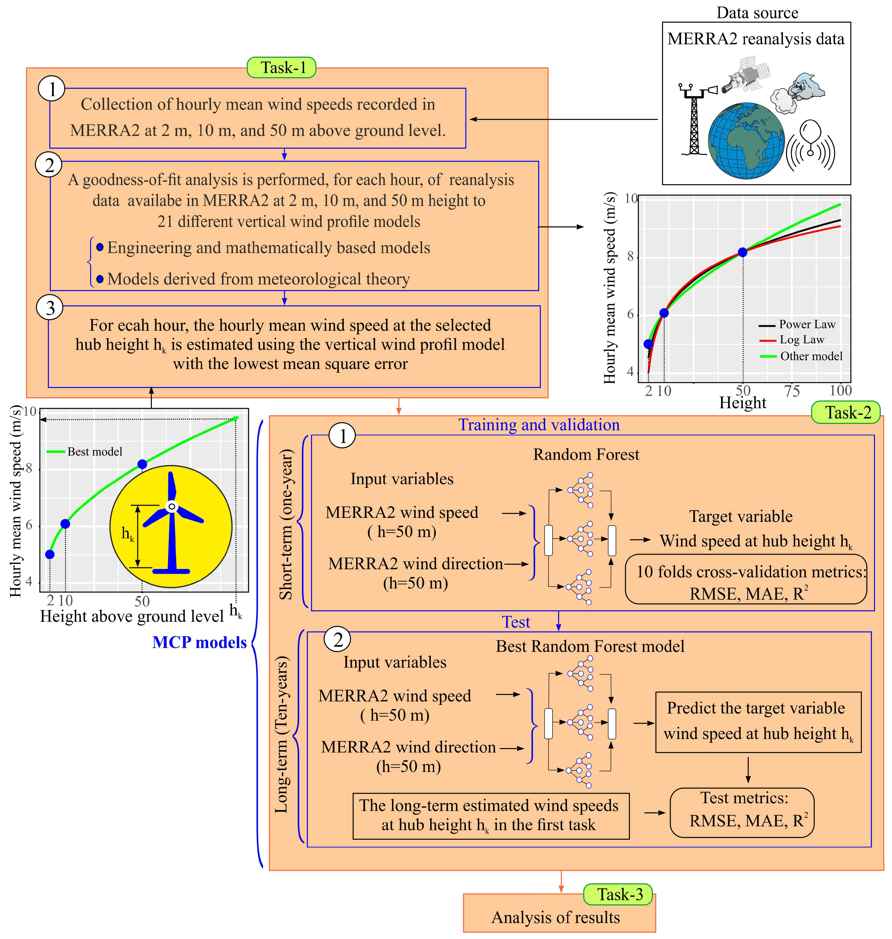
By integrating MCP techniques with ML, this study contributes a robust methodology for transferring MERRA2 wind speeds to wind turbine hub heights, addressing a critical need in wind resource assessment. The methodology was validated in the Canary Archipelago (Spain), selected for its strategic aim of boosting renewable energy use, particularly wind, and thereby reducing external energy dependency. Seven sites representing typical coastal and varied terrain conditions influenced by the predominant NE trade winds are studied.

2. Method

The methodology proposed in this study is structured into three main tasks. First, a set of 21 vertical wind profile models are fitted and evaluated using MERRA2 reanalysis data at 2 m, 10 m, and 50 m heights. Second, a supervised learning approach using RF is employed to build a predictive model that estimates hub-height wind speeds from the reanalysis inputs. Third, the trained model is applied to generate long-term wind speed estimations at typical hub heights and assess its predictive performance. This approach is applied to seven wind-favorable sites in the Canary Islands, selected due to their relevance for current or planned wind farm developments. While geographically limited, these sites are representative of real-world wind resource exploitation scenarios, providing a robust test of the method under typical siting conditions. The methodology has been designed to be replicable and applicable in other regions, particularly those lacking direct measurements at turbine hub height.
A block diagram illustrating the proposed method, covering the process from data collection to result analysis, is shown in Figure 1.
The method comprises three tasks. The first step in Task-1 consists of collecting the wind speeds recorded in MERRA2 at 2 m, 10 m, and 50 m above ground level.
In the second step of Task-1, a detailed goodness-of-fit procedure is applied to the MERRA2 reanalysis dataset, evaluating the performance of 21 vertical wind speed profile models against hourly wind speed data at 2 m, 10 m, and 50 m. This is performed in order to identify the most accurate extrapolation model for each time step. The wind profiles considered range from engineering and mathematically based formulations to those derived from meteorological theory. In the third step of Task-1, for each hour, the wind speed at the selected hub height is estimated using the vertical wind profile with the lowest mean square error. This profile will be considered the optimum profile. In Task-2, the RF-based MCP model is built, trained, validated, and tested. The model is subjected to short-term training (one year) to establish, through supervised learning, the relationship between the hourly mean wind speeds of MERRA2 at 50 m above ground level and the hourly mean speeds estimated at the height of the wind turbine hub in Task-1. Task-2 also calculates the test errors obtained between the long-term (multi-year) predictions of the MCP model and the long-term estimated data using the optimal extrapolation models obtained in Task-1.
Task-3 presents and analyzes the results obtained with reanalysis data for 11 years (2011–2021) from 7 sites in the Canary Archipelago (Spain), which are used as case studies. The heights selected to represent hub heights were 60 m, 70 m, 80 m, 90 m, and 100 m. Each of the tasks and steps are described in greater detail below.

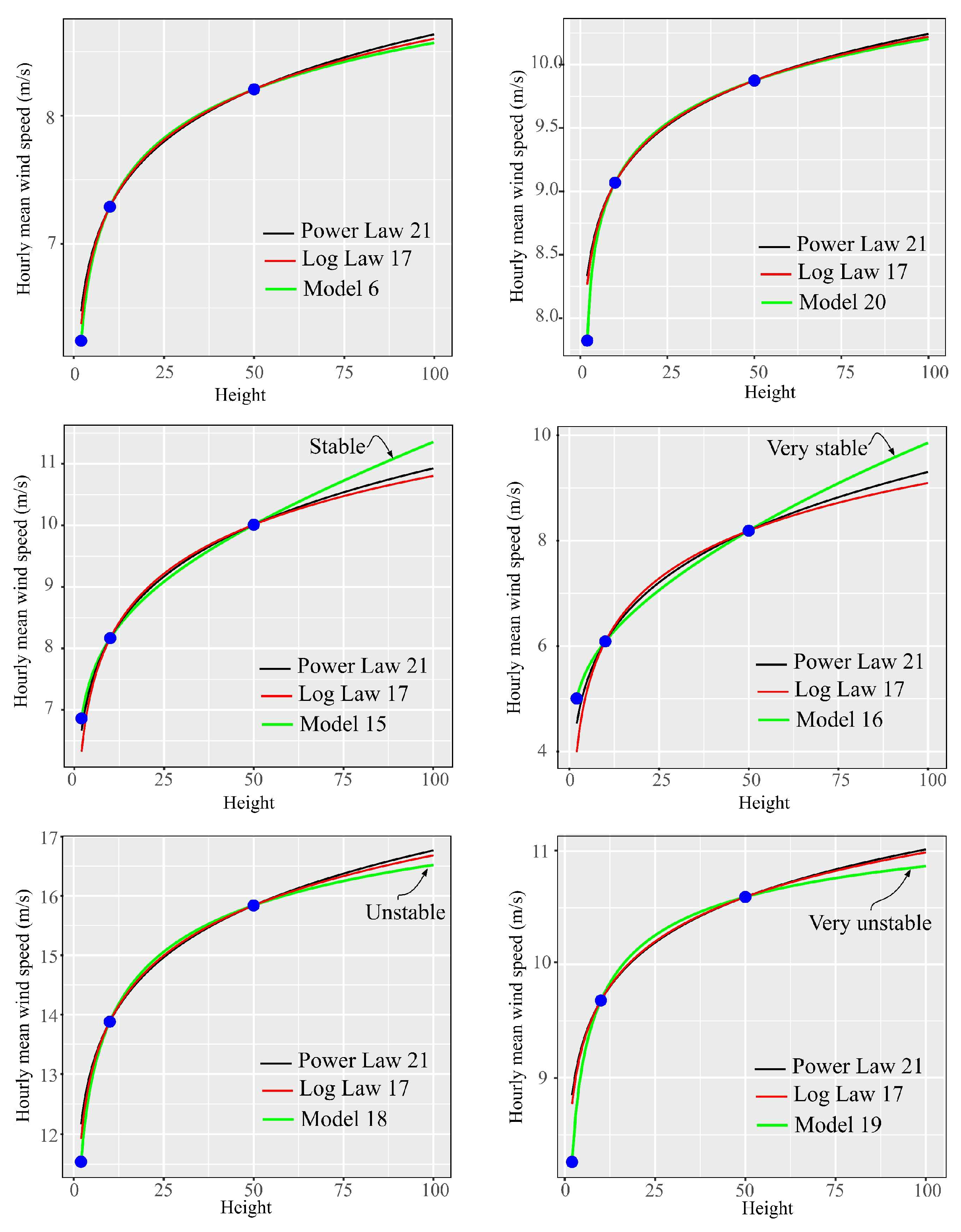
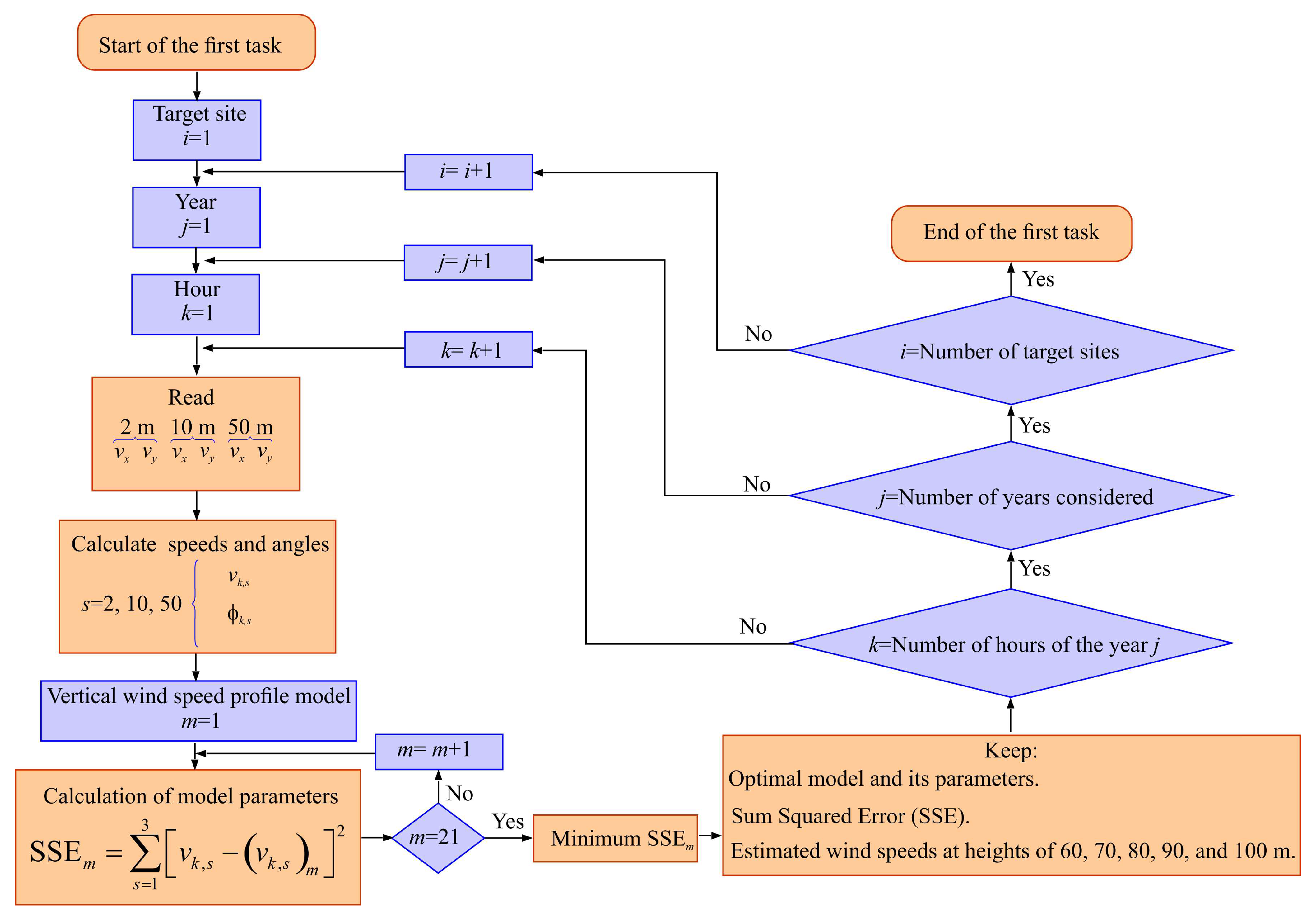
2.1. Task-1: Analysis of the Vertical Wind Speed Models

This task is summarized through the schematic representation shown in Figure 2.
The variable i represents the TS, j the study year, k the time step (hours), and m the vertical wind speed profile considered. In each time step, the variables vx and vy, extracted from MERRA2, are read, which are the x and y components (or longitude and latitude components) at heights of 2 m, 10 m, and 50 m.
The Cartesian components of wind speed (vx and vy) are converted to polar coordinates (v and f). North is defined as f = 0°, and clockwise rotation is considered positive. To calculate v and f, Equations (1) and (2) are used.
v = v x 2 + v y 2
f = tan 1 ( v x v y ) , i f   v y > 0 ,   v x 3 0 p 2 , i f   v y = 0 ,   v x > 0 tan 1 (   v x v y ) + p , i f   v y < 0 tan 1 ( v x v y ) , i f   v y 3 0 , v x < 0 u n d e f i n e d , i f   v y = 0 ,   v x = 0
The analysis of a total of 21 vertical wind speed profile models is proposed (Table 1).
To estimate the parameters q(a, b) of the empirical nonlinear two-parameter models shown in Table 1 and q(A, z0, and L) of the log law model, in stable, very stable, unstable, and very unstable conditions (assigned numbers 15, 16, 18, and 19, respectively; Table 1), the idea is to minimize the sum of squared errors (SSE) function, given by Equation (3). For this purpose, the R 4.4.2 ‘nloptr’ package is used [38], with the ISRES (Improved Stochastic Ranking Evolution Strategy) algorithm.
S S E = v 2 v m h = 2 , θ 2 + v 10 v m h = 10 , θ 2 + v 50 v m h = 50 , θ 2
This method supports arbitrary nonlinear inequality and equality constraints in addition to the bound constraints and is specified within ‘nloptr’ as NLOPT_GN_ISRES. The tolerance used was 1.0 × 10⁻¹⁵, and the maximum number of evaluations was set to 500.
To estimate the parameters q (A, d, z0) of the model designated as model 20 (Table 1), the sequential calculation procedure proposed in [30] was used. In [30], firstly, d (zero-plane displacement) is estimated using the Newton–Raphson method. This is iterated until |dn + 1 − dn| < 0.0001 or until 80 loops is reached. Then, z0 (the aerodynamic surface roughness length) is calculated and, finally,   A = u * k . u* is called the friction velocity and k is the von Karman constant with a value equal to 0.4 [17].
Table 1. Vertical wind speed profile models used. Classification of atmospheric stability according to Obukhov length intervals [39]. y(h/L) is the empirical stability function.
Empirical Nonlinear Two-Parameter (a and b) Models
NumberModelNumberModel
1 v h = 1 + b × ln ( h ) 8 v h = 1 a + b × l n ( h )
2 v h = exp a + b h 9 v h = a × h b
3 v h = 1 a + b h 10 v h = a + b × h
4 v h = a + b × h 11 v h = a + b × e x p ( h )
5 v h = a + b h 12 v h = e x p a + b × l n h
6 v h = a + b × l n h 13 v h = 1 a + b × h
7 v h = a + b × l n h 2 14 v h = a + b h 1.5
Logarithm models based on meteorological theory: Surface layer
NumberModelClass boundariesClass name
15 v h = A × l n h z 0 y h L 200 < L£500 mStable
16 v h = A × l n h z 0 y h L 0£L < 200 mVery stable
17 v h = v r × l n h z 0 l n h r z 0 L > 500 mNeutral
18 v h = A × ln h z 0 y h L −500£L < −200 mUnstable
19 v h = A × ln h z 0 y h L −200£L < 0 mVery unstable
20 v h = A × l n h d z 0 L > 500 mNeutral
NumberThe power law model, an engineering approximation
21 v h = v r × h h r a
The parameter z 0 of the log law model, designated as model 17, was estimated using the wind speeds registered at heights of 10 m and 50 m, shown in Equation (4) [40].
z 0 = exp v 10 ln 50 v 50 ln 10 v 10 v 50
The parameter a (the shear exponent factor) of the power law model, designated as model 21, was estimated using the wind speeds registered at heights of 10 m and 50 m, shown in Equation (5) [13,17].
a = l n v 50 v 10 l n 50 10
Models based on meteorological theory (Table 1) depend on the empirical stability function y(h/L) (Table 2).

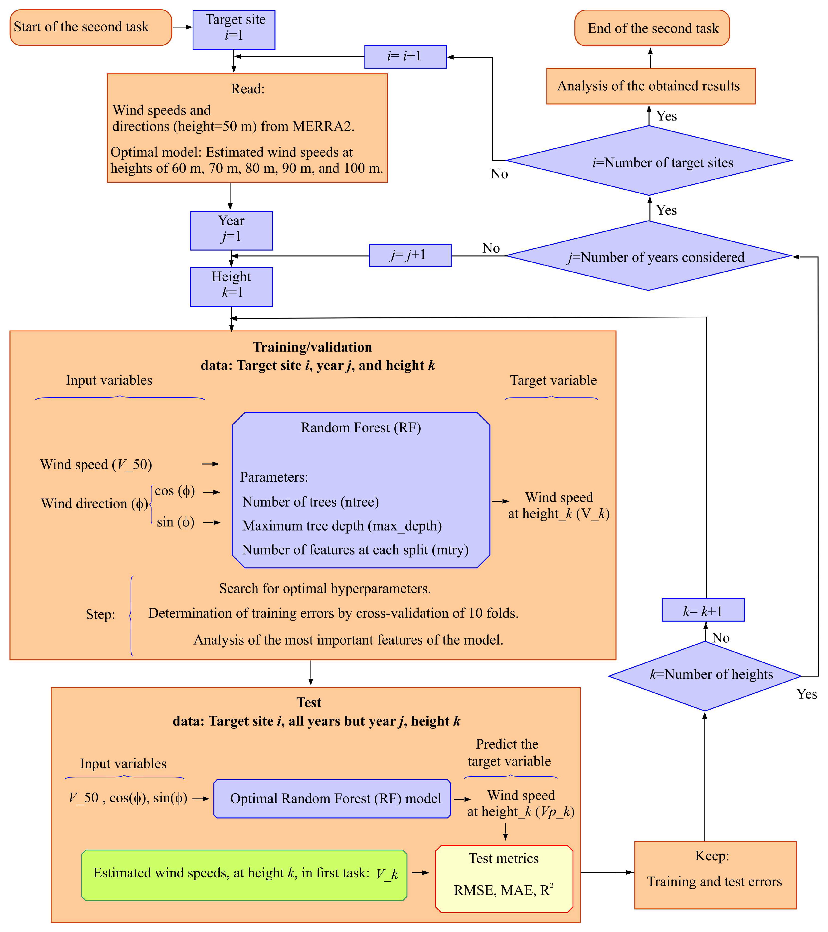
2.2. Second Task: Proposed Machine Learning (ML) Models

Figure 3 shows a block diagram of the second task of the proposed method. For each TS considered (loop i), the data stored during the execution of the first task are read. For each year (loop j) and height (loop k), the training and validation of an ML model is undertaken so that it learns, under supervision, the relationship that exists between the MERRA2 data used as input data and the wind speeds estimated at height k by the optimal models obtained in the first task.
The model for wind speed estimation at height k uses a multiple regression approach, which is represented in Equation (6). In the functional form of the model, X = (X1,X2,X3)T are the input features, the subscript t indicates the instant evaluated, and (vh)t represents the estimated output feature or response.
v h t = f X t = f v 50 t , c o s f 50 t , s i n f 50 t
In this work, the regression function given in Equation (6) is estimated using the RF technique, proposed by Breiman [45]. It was selected for the present study in view of its robustness against overfitting. In addition, in previous studies it was concluded that this technique provides adequate metrics compared to other ML techniques [6,30,46]. Yu and Vautard [9] concluded that RF gave the best simulation accuracy of the three techniques they used for vertical wind speed extrapolation, showing a good performance in temporal and spatial simulation.
In the model proposed here, one of the input features is the wind speed registered in MERRA2 at 50 m. As also considered in other studies [46,47], the wind direction signal, registered in MERRA2 at 50 m, is decomposed into its sine and cosine components, and the angle corresponding to N is taken as angle 0°. The direction feature is introduced to consider the changes in z0 according to wind direction [48].
Given that RFs should not be affected by the presence of highly correlated input features, in this work a feature evaluation was not used, unlike other studies based on other ML techniques [49]. However, an analysis of the importance of the selected features is proposed, as will be seen.
For programming of the RF-based extrapolation model, the randomForest package [50] of the open-source multi-platform R Statistics software (version 4.4.2) [51] was used. RFs are not very sensitive to the choice of hyperparameters used. However, given that the fitting of hyperparameters can help improve performance in RF models, a model tuning via a grid search was used to estimate the hyperparameters of the RF model. The tune_grid() function available in the ‘tune’ package [52] of R Statistics software was used. tune_grid() computes a set of performance metrics, in this case the root mean square error (RMSE), Equation (7), for a pre-defined set of tuning parameters that correspond to a model.
The hyperparameters selected using the expand_grid() function were the number of trees (ntree), the number of features considered at each split (mtry), and the maximum tree depth (max.depth). The first parameter is fitted in this work in the range of 500 to 2000, the second in the range of 1 to the total number of features, and the third in the range of 20 to 50. Although in various published studies [9,47] a proportion of the data is used for training of the RF and the rest for testing, in this study use is proposed of the 10-fold cross-validation criterion which estimates the generalization error more robustly. With this validation, the result is not dependent on the manner in which the partition into two subsets (training and validation) of the complete data sample is carried out. For this purpose, use of the vfold_cv() function, available in the ‘rsample’ package [53] of R Statistics software, is proposed.
The RF model is then trained and evaluated with the best hyperparameters, and the most important features to the model are determined. For this, the permutation feature importance measurement is used, which was introduced by Breiman [45] for RFs.
Once the RF model has been defined, the long-term wind speed prediction at height k is undertaken using the predict() function, available in the ‘randomForest’ package [50] of R Statistics software. ‘Long-term’ is taken as all the years in the study except for the year j used to train and validate the RF model. With the predicted wind speeds and the long-term estimated wind speeds in the first task, it is then proposed to calculate the test metrics, in this case the RMSE, Equation (7), and the mean absolute error (MAE), Equation (8),which have previously been used in methods to estimate hub-height wind speed based on RF [30,53]. The coefficient of determination (R2), Equation (9), is also considered, which has also been used previously in these methods [54] and in MCP techniques [44,47] where the procedure is similar to that proposed in the present work. RMSE is used to evaluate large deviations, while MAE is more robust to outliers. In this task, R2 serves as a measure of how much of the variability in the TS data is explained by the reanalysis data.
In Equations (7)–(9), yi is the observed (true) value, y ^ i is the predicted value, and n is the total number of observations.
R M S E = 1 n i = 1 n y i y ^ i 2
M A E = 1 n i = 1 n y i y ^ i
R 2 = 1 i = 1 n y i i = 1 n y i n 2 i = 1 n y i y ^ i 2

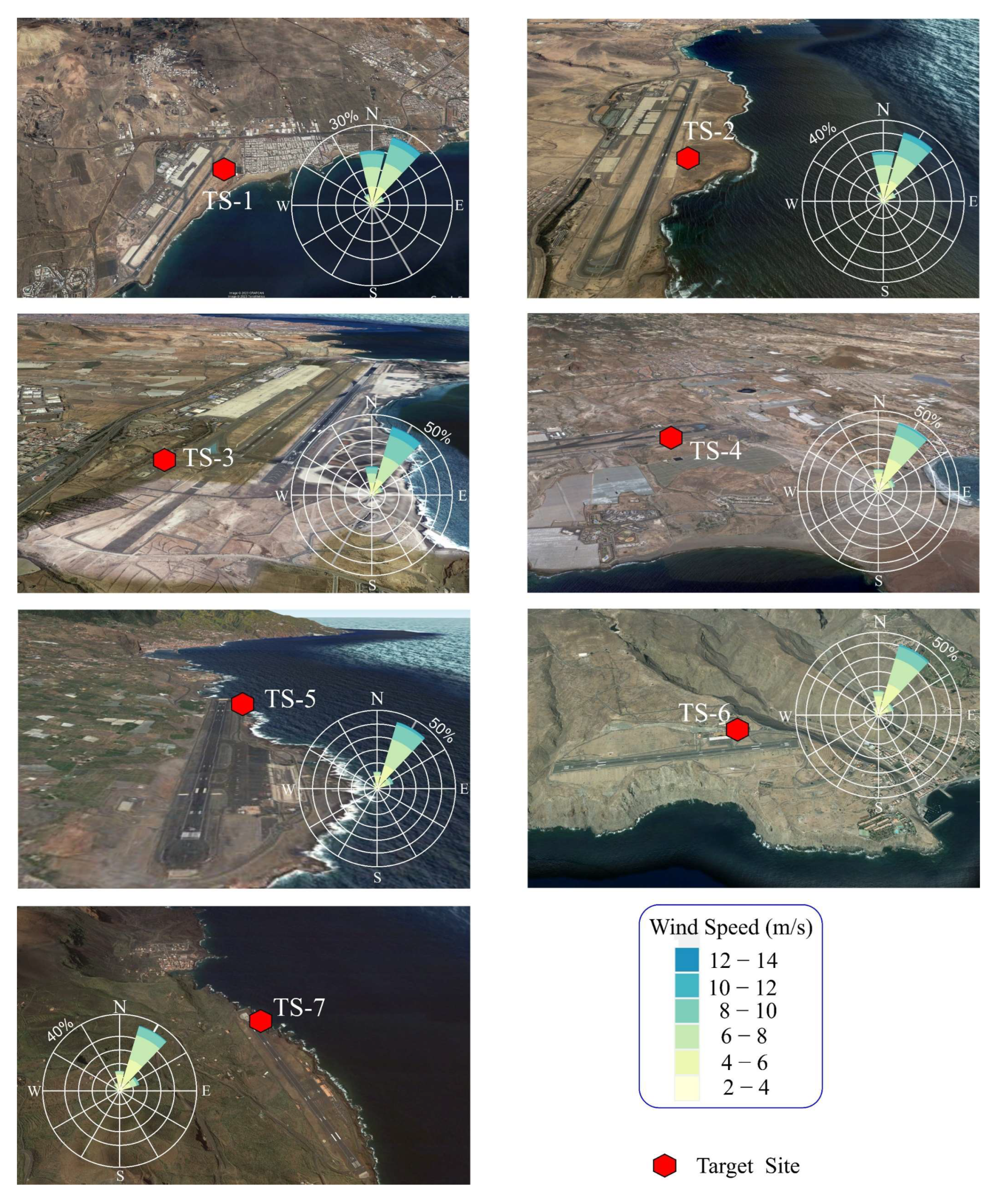
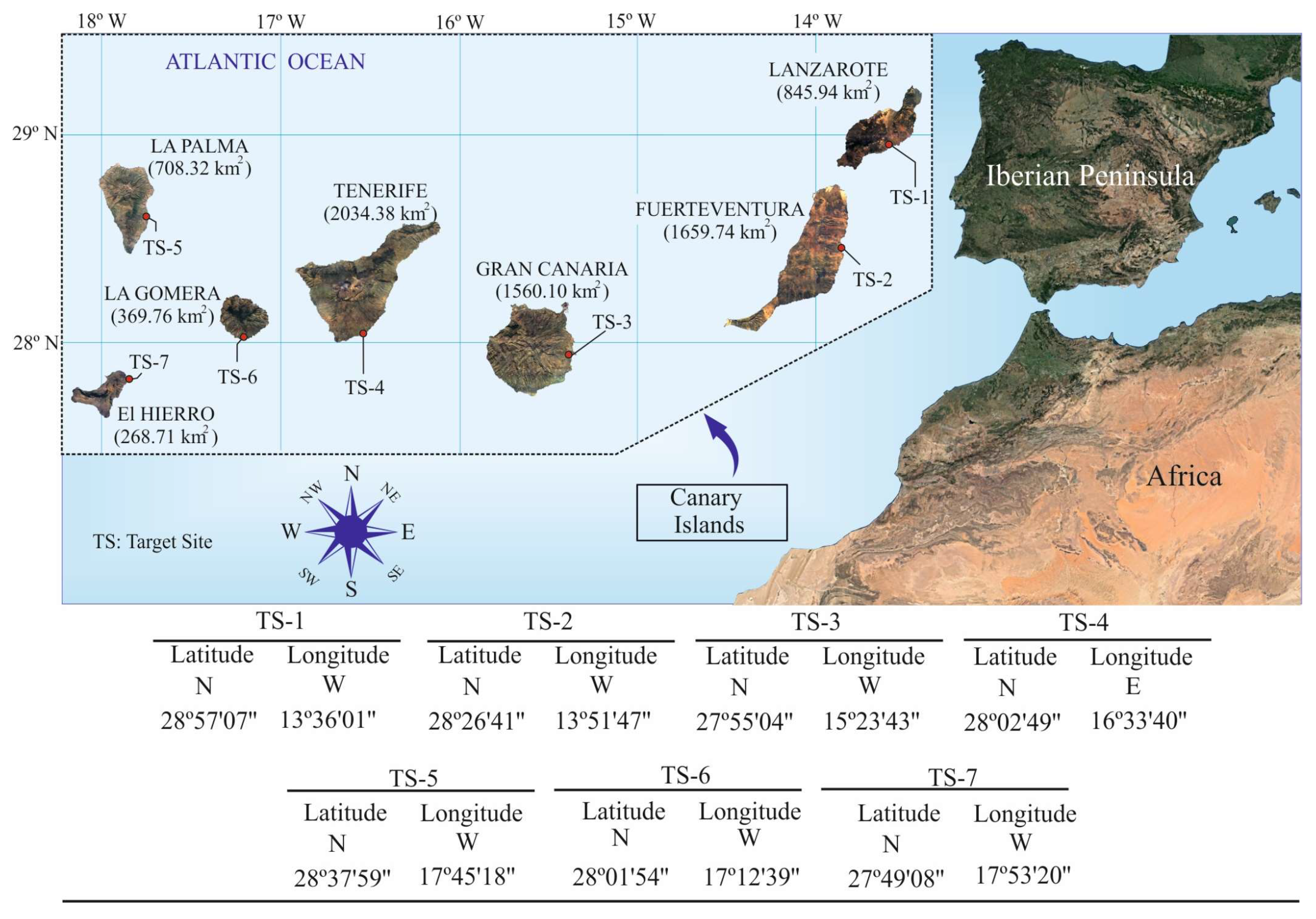
3. Case Study: Canary Islands

To verify the utility of the MCP model, the Canary Archipelago (Spain), which comprises seven main islands (Lanzarote, Fuerteventura, Gran Canaria, Tenerife, La Palma, La Gomera, and El Hierro), was selected. This archipelago is situated northwest of the African continent (Figure 4). In order to reduce external energy dependency and combat climate change, the autonomous Canary Islands Government has established a strategy targeted at maximizing the exploitation of renewable energies through the promotion of wind farm installations, principally in the coastal areas of the E and SE. In this context, as a case study, seven TSs were selected, the coordinates of which are shown in Figure 4.
The area surrounding the selected TSs and their wind roses is shown in Appendix A.1 (Figure A1). The predominant NE wind direction is typical of the trade winds crossing the Canary Archipelago [55]. Given the location of the TSs, for most of them the surface properties upstream of the site for which the wind profile is intended to be estimated are those typical of the open sea. However, in other directions, although with lesser frequency, the roughness length will be higher given the characteristics of the terrain (open plane, grass, some isolated obstacles) upstream of the TS.
Using a boxplot representation, Figure 5 summarizes the distribution and variability of the MERRA2 mean monthly wind speeds at heights of 2 m, 10 m, and 50 m, over eleven years (2011–2021) at the seven selected sites (TS-1 to TS-7). The calculated mean monthly wind speeds of the TSs at 10 m above ground level during the considered period of analysis are in the interval 5.3 m/s to 6.7 m/s. As can be seen, the frequency histograms of the mean monthly wind speeds are notably symmetrical, and so the mean and the median (Q2) speeds have similar values.

4. Results and Discussion

The results obtained in the two tasks outlined in the Section 2 are presented and analyzed in this section.

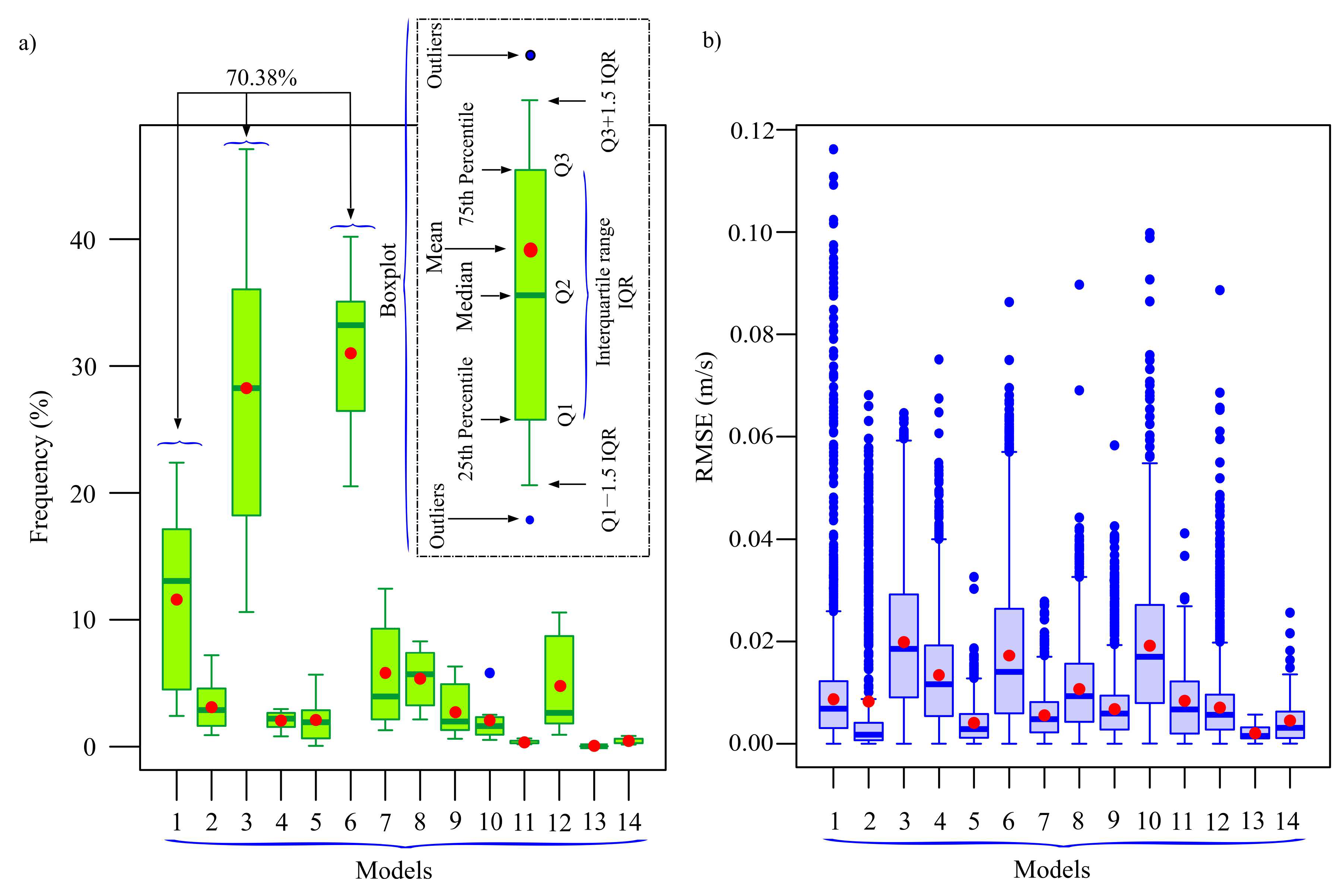
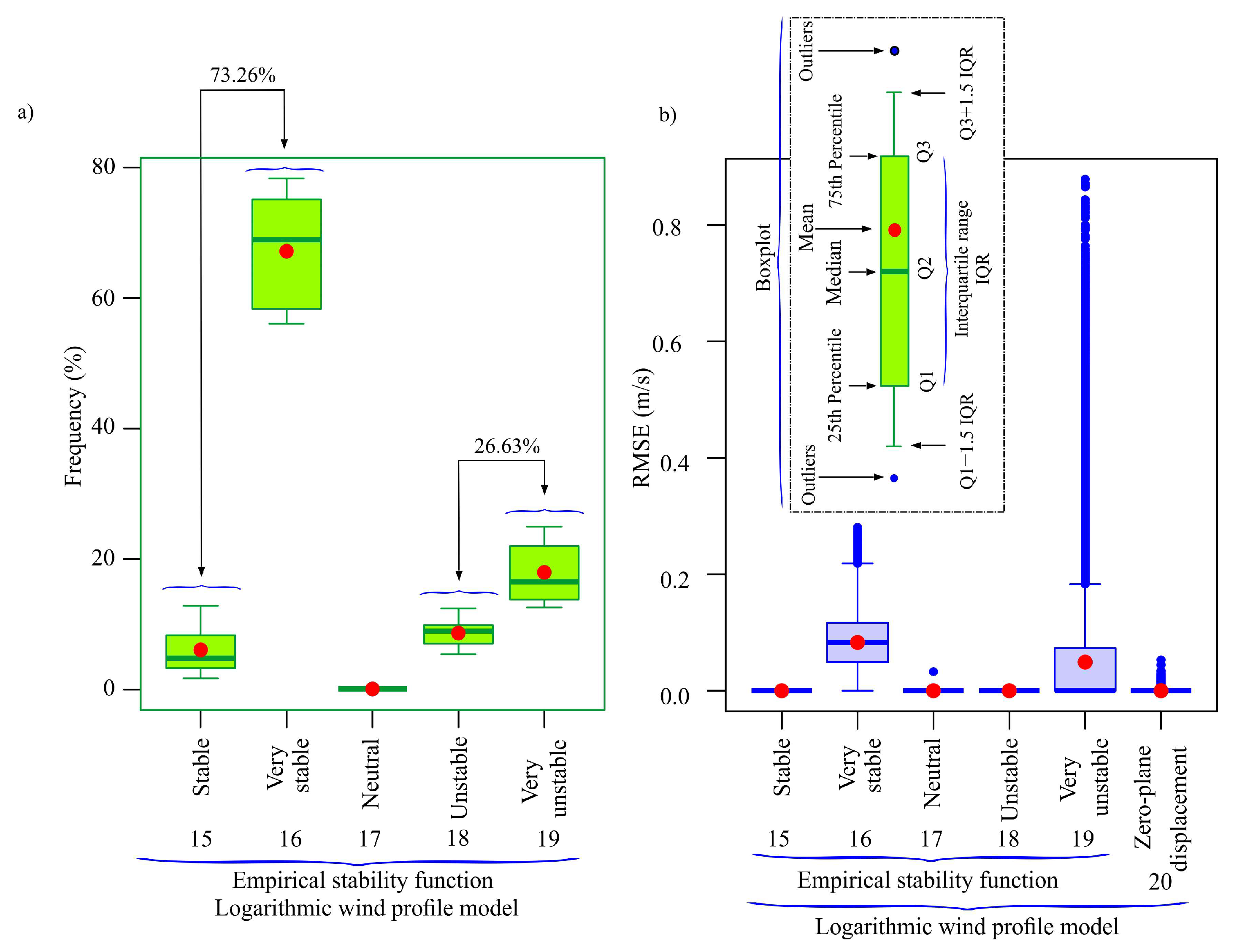
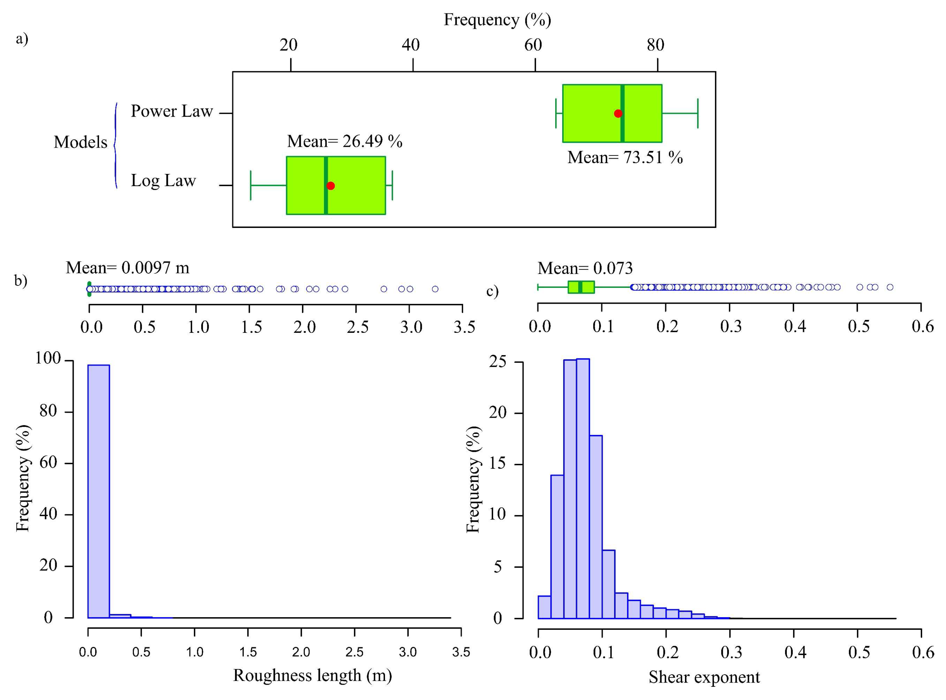
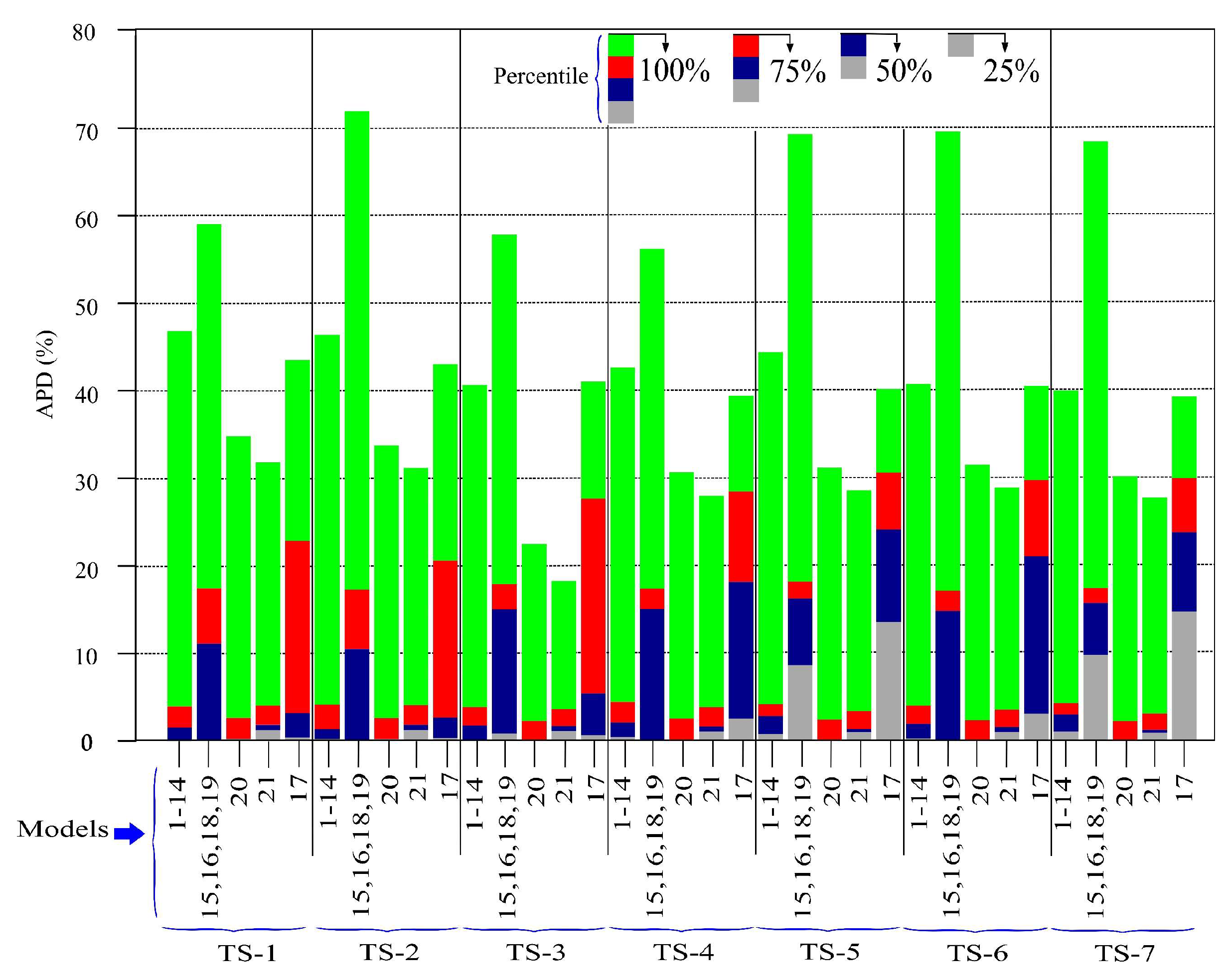
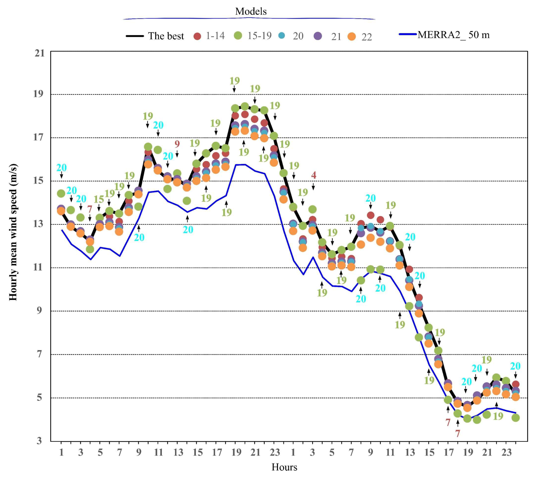
4.1. First Task: Analysis of the Vertical Wind Speed Models

Figure 6 shows the best-fit frequencies of the 21 vertical wind speed models indicated in Table 1. That is, the models are compared according to the percentage of times that they best fitted the mean hourly wind speeds registered at three heights in MERRA2.
As can be observed in Figure 6, the logarithmic wind profile model of three parameters (model 20), which includes the zero-plane displacement and the assumption that the atmosphere is neutrally stratified, fitted the MERRA2 data with the highest mean frequency (51.31%). The log law models which take into account the stability function also present a high mean frequency (26.38%) of best fit, with a slight prevalence, for the TSs of the study, of unstable vs. stable conditions. The two-parameter models proposed in this paper were the best-fitting models in 19.44% of the cases. However, the models of just one parameter (17 and 21), extensively used in the literature [13,20,40] because of their simplicity (log law and power law), presented a very low frequency of best fit.
Figure A2 (Appendix A.2) shows the results obtained in the first task with the 14 nonlinear two-parameter empirical models listed in Table 1. As can be seen in Figure A2, 3 of the 14 models (3, 6, and 1) fit the MERRA2 data with a high frequency compared to the remaining 11. The mean relative frequency of best fit of the three models taken together was 70.38%. It should also be noted that practically half of the models (11,13,14,9,4,5) analyzed adequately fitted the MERRA2 data (see Appendix A), but their relative frequency of fit was very low.
The log law models that include the empirical stability function depend on three parameters and are more complex than the previously discussed nonlinear two-parameter models. However, they can provide information about the atmospheric stabilities. As can be seen in Figure A3 (Appendix A.3), the ‘very stable’ and ‘stable’ atmospheric conditions occur with a mean relative frequency of 73.26%. The ‘very unstable’ and ‘unstable’ conditions present with a mean frequency of 26.63%.
More detailed information on the best-fit frequencies of the power law model and the logarithmic law model is shown in Appendix A.4. Histograms and boxplots of the roughness length and shear exponent are also shown. As can be seen in Figure A5, the power law and log law models perfectly fit the wind speeds registered at 10 m and 50 m, as their parameters (a and z0) were estimated with Equations (4) and (5) so that this would occur. However, on many occasions, these models present difficulties when it comes to the MERRA2 wind speeds registered at 2 m height.
It should be noted that Equation (4), proposed in the literature to estimate z0, gave some outliers of more than 3 m (see Appendix A.4), usually assigned to a city with tall buildings [56] and not corresponding to the surroundings of the TSs of the study. Likewise, Equation (5), proposed in the literature to estimate a, gave some outliers (see Appendix A.4) that do not correspond to the surroundings of the study TSs. These parameters suggest that these models, although they fit MERRA2 data at two heights (10 m and 50 m), are not always adequate to represent the wind profile.
A comparative analysis of the absolute percentage differences (APDs, Equation (10)) between the wind speeds (Vt) and wind power densities (WPDt, Equation (11)) estimated by the models with the best fit (B) to the MERRA2 data and those estimated by the rest of the models allows us to evaluate the magnitude of these differences and their practical importance.
A P D t V = V t B V t o t h e r s V t B × 100 ;   W P D t V = W P D t B W P D t o t h e r s W P D t B × 100
W P D t = 1 2 × r × ¯ V t 3
Figure 7 shows the quantiles of the APDs when estimating the WPD at 100 m height for the seven TSs. As can be seen, the values of the quantiles depend on the characteristics of the TS. However, it should be noted that in all of them the APDs of the WPD can be considerable (Q4 with values close to or even above 70%) if an inadequate vertical extrapolation model is selected. In this context, it is proposed to select in each hour the vertical wind speed profile model that best fits the MERRA2 data at three heights. Additional information on these estimated differences at three heights (60 m, 80 m, and 100 m) is shown in Appendix A.5.
Figure 8 illustrates the hourly selection of the best-fitting vertical wind speed profile models at 100 m height for TS-1 over two consecutive days (23–24 February 2020). The black line traces the optimal model selected each hour based on the minimum MSE. The figure also includes the MERRA2 wind speeds at 50 m as a reference. This visualization highlights how suboptimal model choices can lead to underestimation of wind speeds at hub height, sometimes even falling below the original MERRA2 value at 50 m. This emphasizes the importance of dynamically selecting the most appropriate model at each time step.

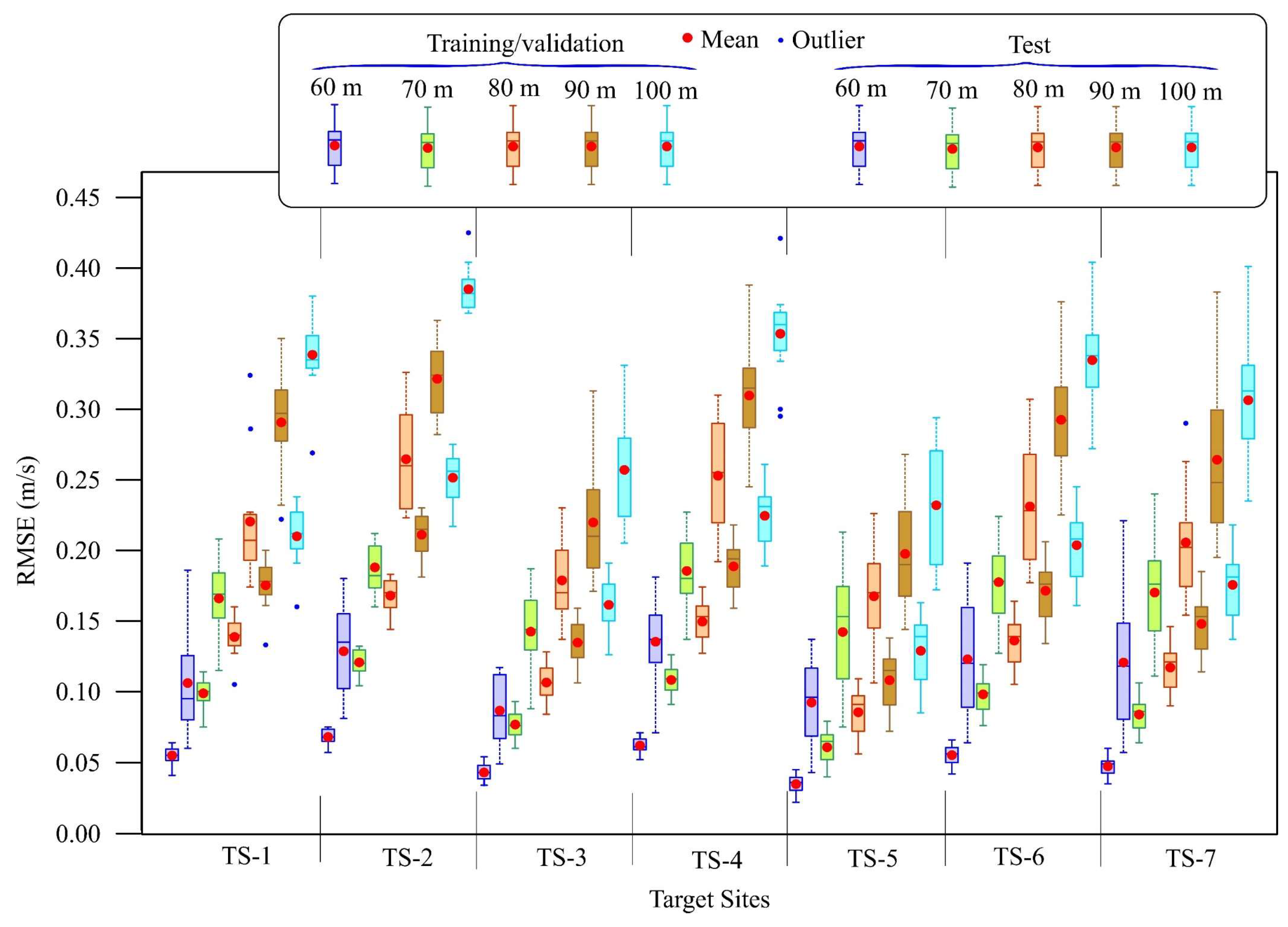
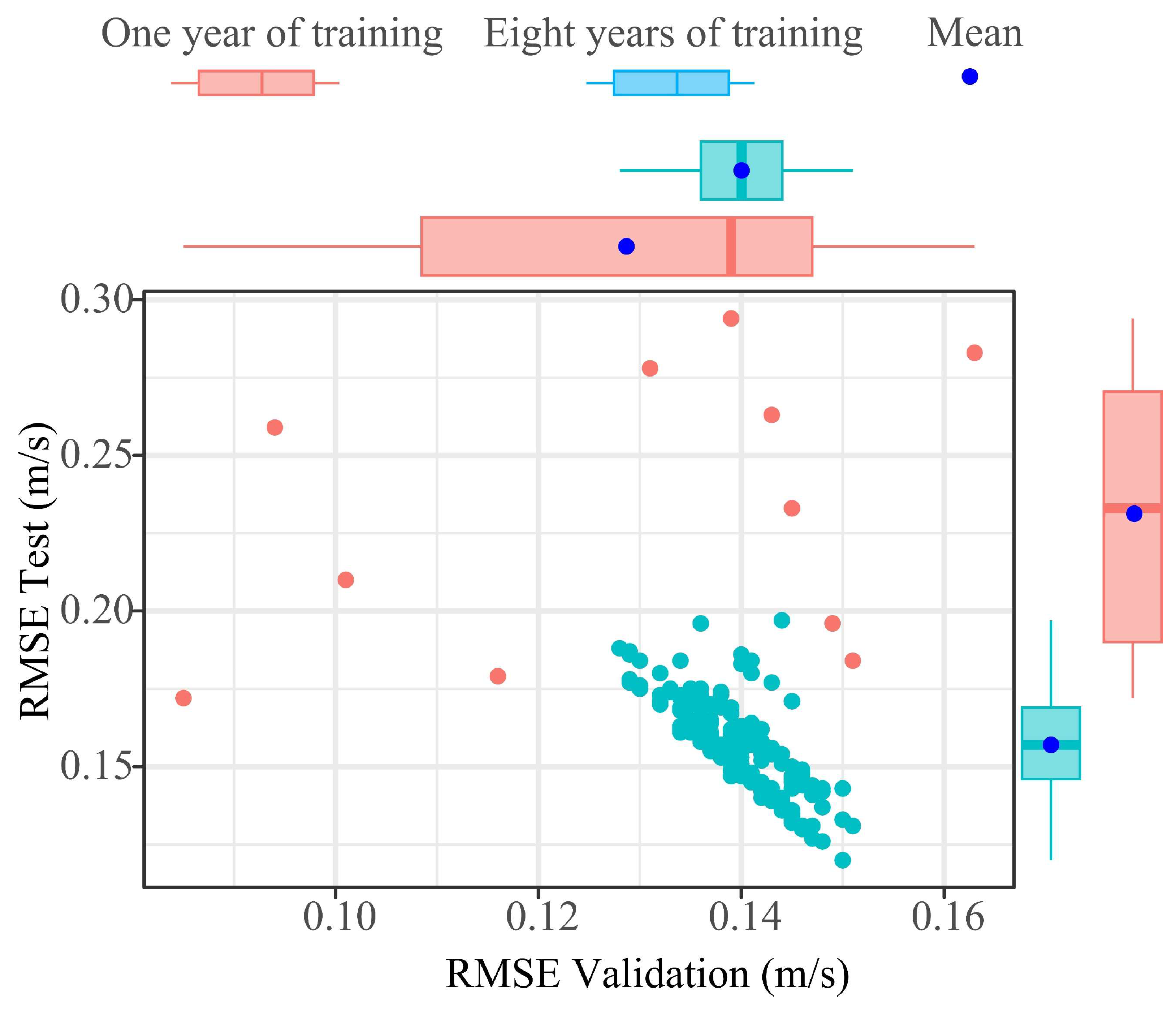
4.2. Second Task: Performance of the Proposed Machine Learning Model

It can be deduced from the analysis of the RF models that there were no significant differences between the values of the optimal parameters. That is to say, with the three input features used, the most frequently obtained values of mtry, ntree, and max_depth were 2, 2000, and 20, respectively, with, in most of the models, stable RMSE values.
It can also be deduced from the analysis of the importance of each of the input features in vertical wind speed prediction, as can be seen in Appendix A.6, that the feature of greatest importance is wind speed registered at 50 m height (V50). This concurs with the results obtained by Yu and Vautard [9] and Optis et al. [47]. In other words, in this case, the removal of V50 would result in the highest percentage decrease in accuracy.
The most frequently selected values for ntree, mtry, and max_depth were 2000, 2, and 20, respectively. These values were obtained through a grid search optimization using 10-fold cross-validation, and they consistently provided stable and low RMSE values across all sites and heights. Their repeatability and alignment with values used in prior studies suggest that they are suitable for the proposed modeling task.
The wind direction, decomposed into its sine and cosine components, is the second most important feature, but it was found not to influence the predictive capacity of the models when the 10-fold cross-validation was performed.
The boxplots of the RMSEs of the 10-fold cross-validation which were obtained when evaluating the trained models are shown, for each TS and extrapolation height, in Figure 9. Figure 9 was generated by the authors based on the results of the models developed in this study. Also shown in Figure 9 are the RMSEs obtained in the tests.
From the analysis of the validation errors (Figure 9), it was found that the validation RMSEs were always lower than 0.275 m/s at the 100 m height, independently of the year of the data used to carry out the training/validation of the models.
Although 10 years were used to carry out the tests, the maximum RMSEs (outliers), obtained in TS-2, were lower than 0.425 m/s at the 100 m height (Figure 9). For purposes of comparison, it should be noted that in the study carried out by Yu and Vautard [9], in which they used a long data series with intervals of three hours for the training (22 years) and validation (3 years) and a short test series, the mean test RMSE value in the region considered in their study was 0.525 m/s. This reflects the capacity for generalization of the RF models trained in the present study to represent the profile of wind variation with height with minimum error, using a reduced number of data to carry out their training/validation.
The MAE values of the tests, which are lower than the RMSE, are shown in Appendix A.7. The maximum value at 100 m height was 0.262 m/s (at TS-2). The lower MAE values are due to the fact that the MAE metric is more robust than the RMSE and that the MAE metric does not give as much importance to outliers as the RMSE. The test R2 results are also shown in Appendix A.8, where it can be seen how they decrease with extrapolation height but still maintain high values. The smallest R2 at 100 m was an outlier of 0.972 (TS-7), indicating that at least 97.2% of the target feature is predicted by the model in the case considered.
Methods that use ML techniques, like MCP methods, are based on the assumption that the data are statistically stationary [12]. That is, the effects of climate change are ignored, and it is assumed that the behavior of the wind is similar in other years. Therefore, one option to even further reduce the prediction errors of the models is to use a sample with a larger number of years of data for the training. In this way, a more varied set of data could be obtained which represents interannual variations. For the case of MCP methods, Taylor et al. [57] concluded that the results obtained in their study provide evidence that there is a significant seasonal influence on the quality of the long-term estimations. In consequence, they highlighted the importance of having at least 12 months (or multiples thereof) of measurements for the target site. According to Miguel et al. [58], the studies that they undertook showed increasing reductions in the uncertainty of the prediction when adding one, two, three, and four years to a two-year series.
Figure 10 shows, by way of example, the validation and test RMSE boxplots of TS-5 at 100 m height when employing just one year and when employing eight years of data for the training and 10-fold cross-validation. When long-term training (LTT) was used, short series of three years were used to carry out the test, as also done by other authors [9]. A total of 165 series of eight years were used to carry out the training and 10-fold cross-validations. These series comprise the 165 combinations (without repetition) of eight of the eleven years available (2011–2021). The three remaining years of each of the 165 series were used to carry out the tests.
As can be deduced from Figure 10, the test RMSEs decrease when using LTT compared to those produced when using short-term training (STT). The percentage of relative variation in the mean training RMSE between the two types of models is 8.4%, while the percentage of relative decrease in the mean RMSE when using LTT reaches 32.4%. This could be considered a high percentage, but, in absolute values, the reduction is just 0.075 m/s (=0.2319 m/s − 0.1568 m/s). This means that in the case of considering an air density of 1.225 kg m−3, the mean absolute difference in WPD estimation is 0.037 kW/m2.
Appendix A.9 shows, for the case of TS-5 at 100 m height, the boxplots of all the test metrics of the models based on one year and eight years of training/validation. These metrics correspond to the wind speed and the WPD feature. In all of them a decrease can be observed in the MAE and RMSE error metrics and an increase in R2. However, the absolute values of the metrics do not differ substantially between the two types of models, and the R2 values of the models with one year of training show that a high percentage of the target feature is predicted by the model in the case considered.
A comparison is shown in Figure 11 of the mean hourly power output (estimated through Equation (12) [4]) that an ENERCON E-70 wind turbine (2300 kW rated power) [59] would have generated if operating with the wind speeds estimated by the RF models and with the TS-5 target (La Palma Airport, Spain) it wind speeds at 100 m height.
P t = 1 2 × r t × c p l , b × S × v t 3
The power Pt produced by a WT in an instant t, Equation (12), depends on the wind speed vt at hub height, the rotor-swept area S, and the air density rt and its power coefficient cp, which is a function of the tip speed ratio l and the pitch angle b [4].
Figure 11 shows, by way of example, 700 h in 2015 not used by any of the models in their training.
In the estimation of the power output using Equation (12), a constant air density over time is assumed, using the mean value corresponding to the study area. This simplification is considered appropriate given that wind speed, which exhibits greater temporal variability and relative magnitude, has a dominant influence on wind power output. Moreover, this assumption is commonly adopted in studies focused on the preliminary assessment of wind resources and the identification of potentially suitable sites for wind turbine deployment. Therefore, any errors introduced by this assumption do not significantly affect the comparative validity of the results presented.
It is important to note that the wind speed data used in this study, derived from the MERRA2 reanalysis dataset, have an hourly resolution. While this temporal resolution does not capture short-term wind fluctuations, it is commonly used and accepted in preliminary assessments of wind resource potential at regional or mesoscale levels. For detailed design and dynamic modeling of wind turbines or wind farms, higher-frequency wind measurements would be required.
It can be seen that the target values of power output and the predicted values at 100 m height are in close agreement. When the years 2015, 2016, and 2020 were simulated, the RMSE and MAE obtained with the model trained with eight years of data were 36.91 kW and 14.74 kW, respectively. In the case of using the model with one year of training, the RMSE and MAE were 40.89 kW and 17.62 kW, respectively. It can be seen how the difference between the errors produced by the two models is not large. The magnitudes of these errors are lower than those published in works on the estimation of wind turbine output power using soft computing models [60]. In order to provide a fairer comparison with other studies using wind turbines with different rated powers, the RMSE and MAE values obtained in this study have also been expressed as percentages of the turbine’s rated power (2300 kW). For the model trained with eight years of data, the RMSE and MAE correspond to approximately 1.6% and 0.64% of the rated power, respectively. In contrast, a referenced study using a 3300 kW turbine [60] reported normalized errors of 2.38% (RMSE) and 1.48% (MAE). These results highlight the relatively strong predictive performance of the models developed in this work.
In the case study, the use of RF techniques with one year of data for training/validation can be considered acceptable. However, it should be noted that, if a large number of years is required for the training and validation (because the short-term training models generate inadmissible errors), the ML-based extrapolation method would lose its advantages. That is, the peculiarities of these models (in terms of reduction in the time employed in the MERRA2 data processing tasks and in model selection computing in the first task) would be lost given that long-term data series, following the strategy established in the first task, would also need to be obtained.

5. Conclusions

This study proposes a Measure–Correlate–Predict (MCP) strategy to transfer hourly mean wind speeds at 50 m above ground level from MERRA2 reanalysis to wind turbine hub heights. Seven target sites in the Canary Archipelago were selected as case studies. The key conclusions derived from the analysis are as follows. These findings have been consistent throughout the case studies, which have shown different geographical and environmental contexts:
Among the range of vertical wind speed profile models analyzed, the following is shown:
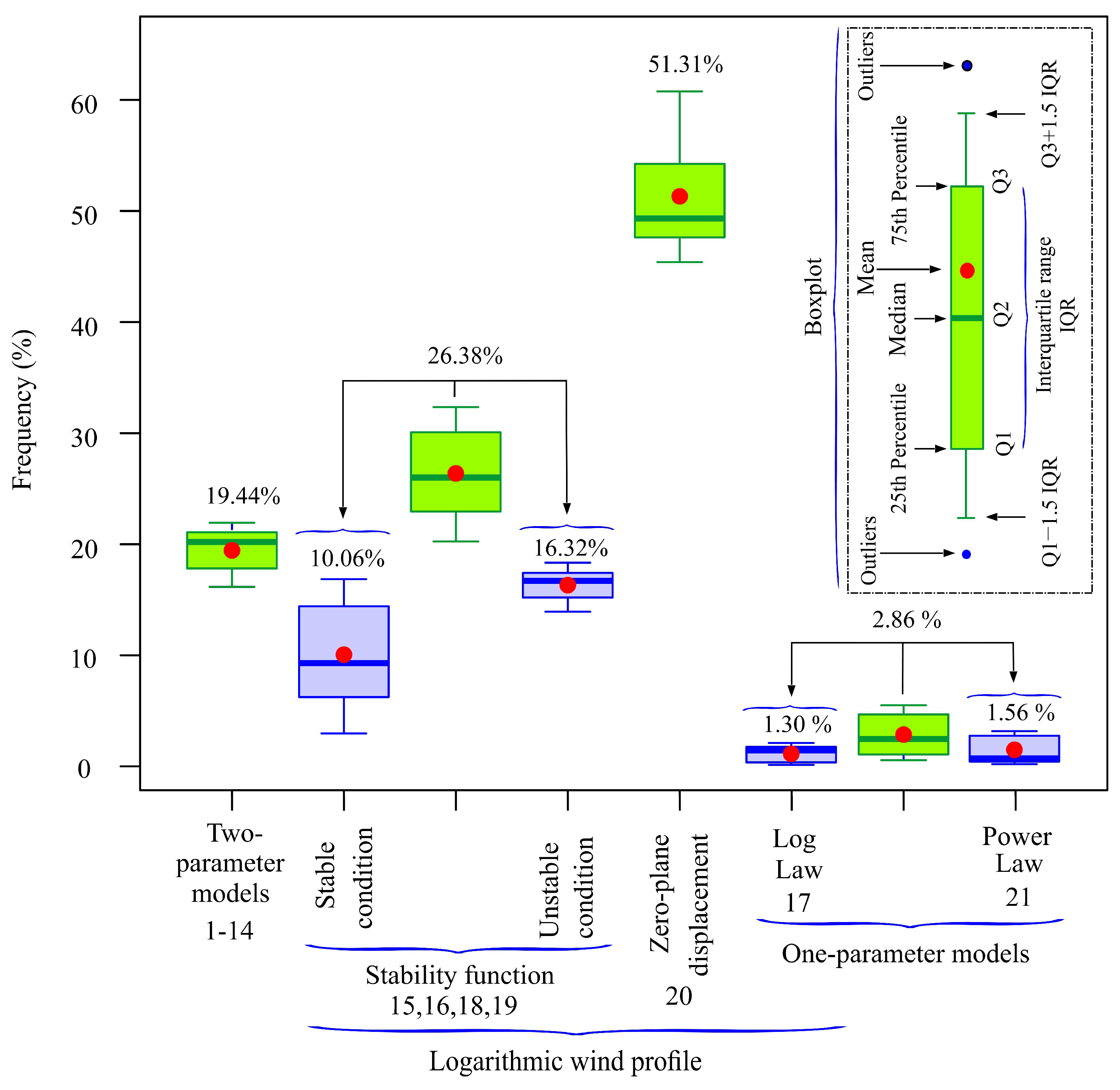
  • The three-parameter logarithmic wind profile model, which incorporates zero-plane displacement and assumes a neutrally stratified atmosphere, demonstrated the best fit to the MERRA2 data, with the highest mean frequency (51.31%).
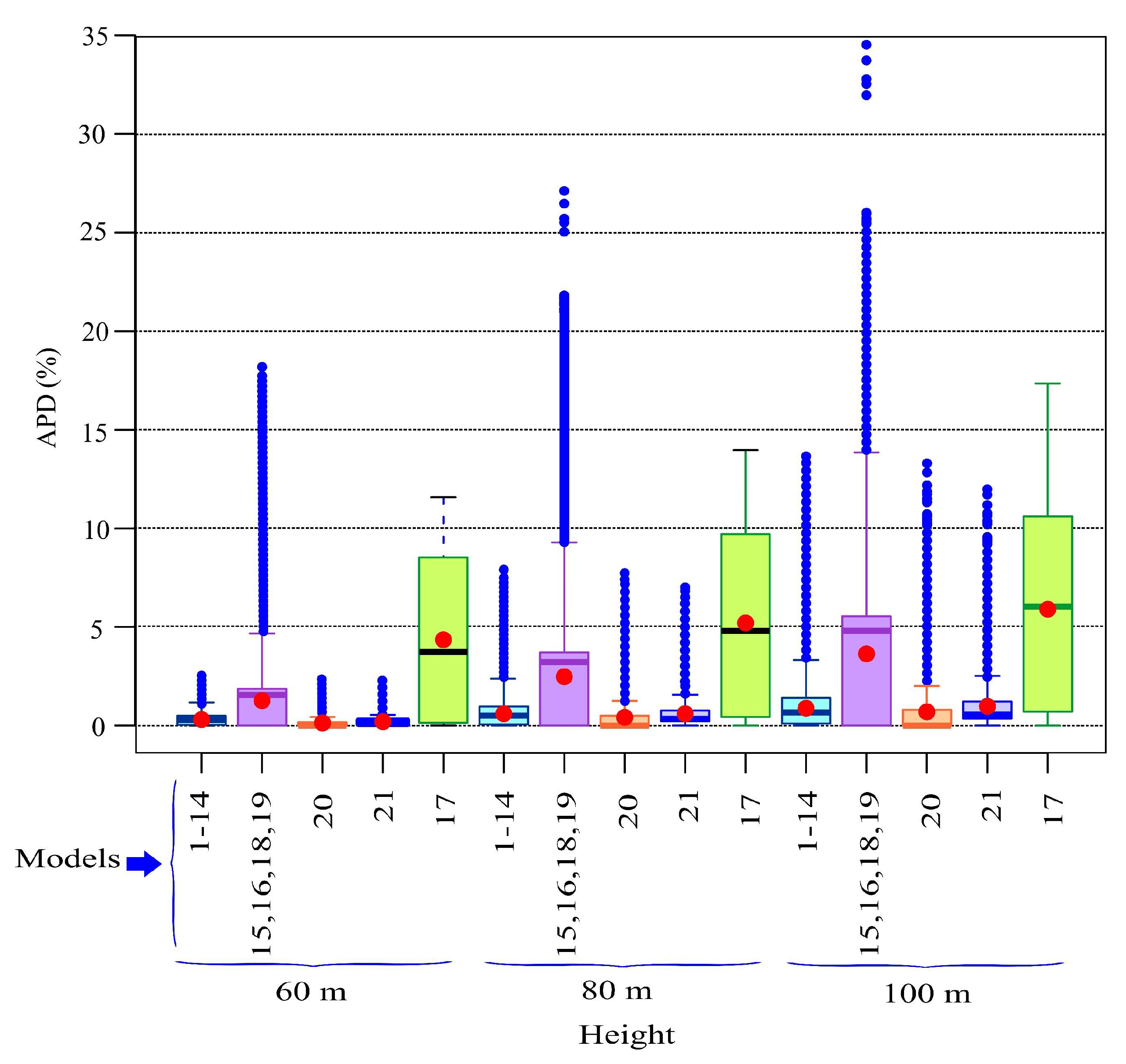
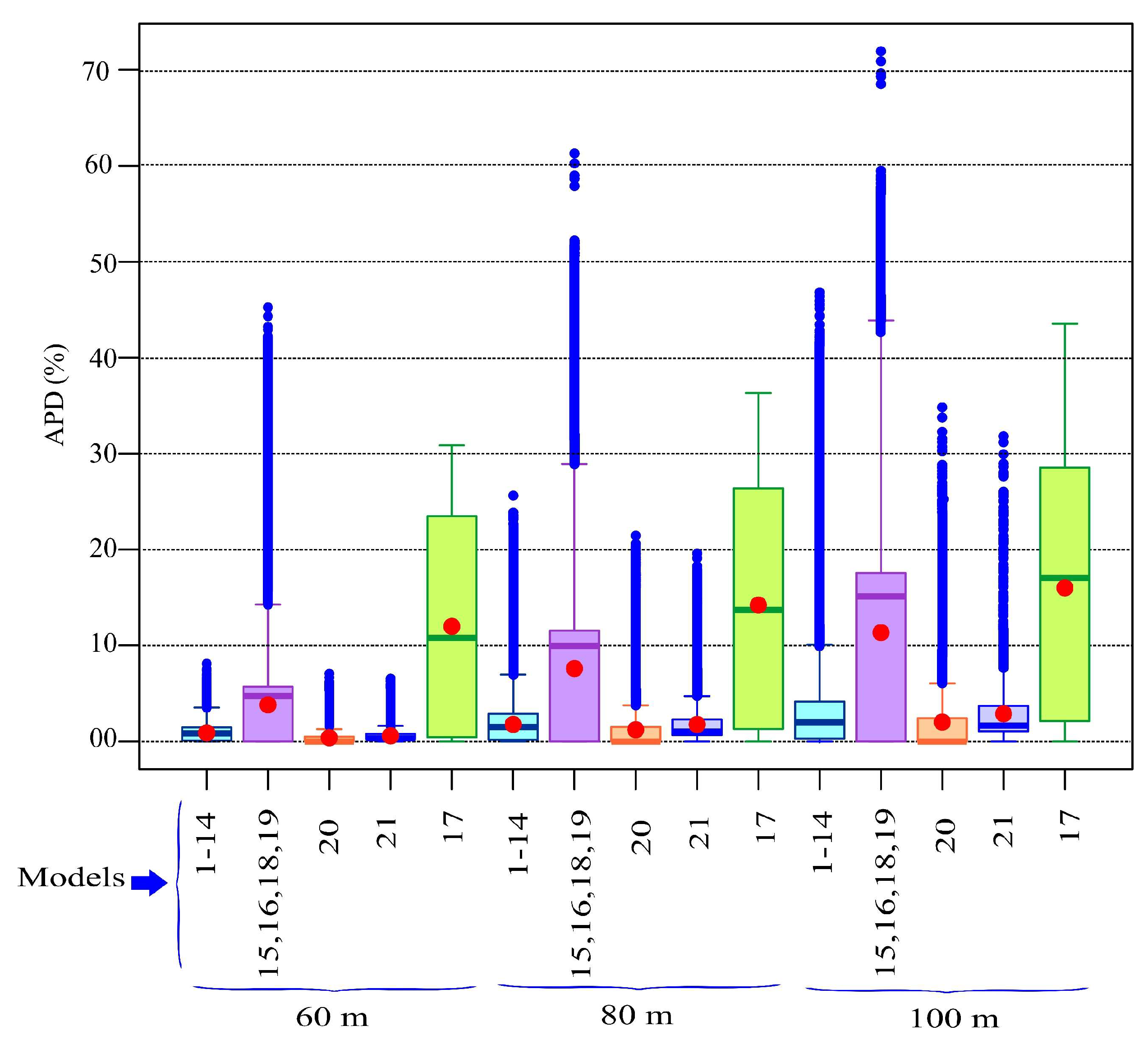
  • The fourteen two-parameter vertical wind speed profile models proposed in this study provided the best fit to the MERRA2 data in 19.44% of cases.
  • The single-parameter vertical wind speed profile models (e.g., power law and log law), widely employed in the literature, showed very low best-fit frequencies in the case study. Additionally, non-representative outliers for the surface roughness length and shear exponent factor were identified when these parameters were estimated using MERRA2 wind speeds at 10 m and 50 m heights.
  • To minimize significant errors in vertical wind speed estimations, and consequently in wind power density and wind turbine power output estimations, it is recommended to select, at each time step, the vertical wind speed profile model that best fits the available MERRA2 wind speed data at 2 m, 10 m, and 50 m heights.
For the performance of the RF-based MCP model, the following is shown:
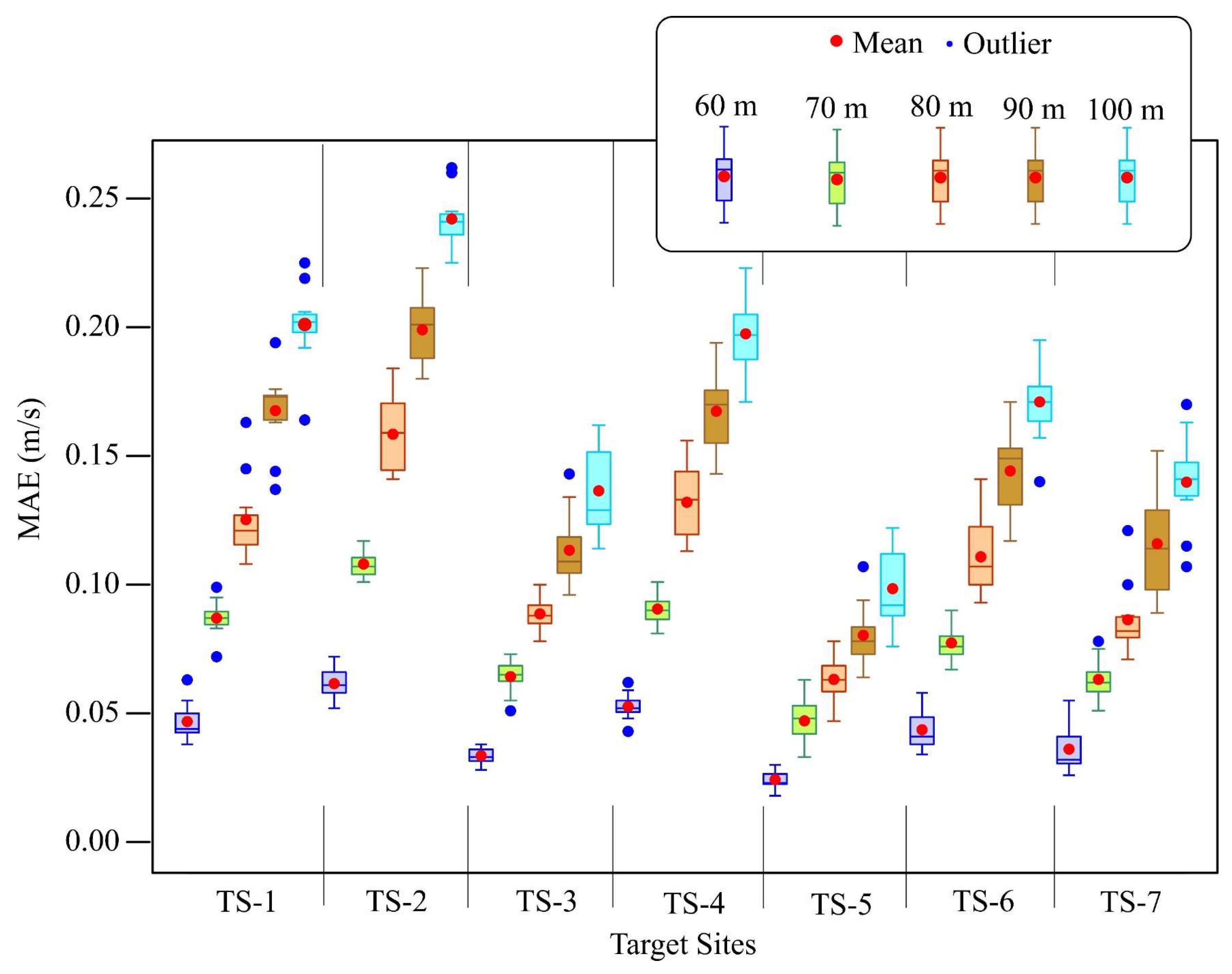
  • In applying the RF-based MCP strategy, trained with short-term (one-year) supervised learning, the methodology achieved strong predictive performance. Tested with 10 years of data, RF-based predictions at 100 m hub height yielded a maximum RMSE (outliers) below 0.425 m/s.
  • These results underscore the effectiveness of combining MCP techniques with ML in significantly improving the accuracy of wind speed estimations at wind turbine hub heights.
These findings not only demonstrate the effectiveness of the proposed MCP strategy but also emphasize the critical role of advanced ML techniques and optimized vertical wind speed profiles in improving wind resource assessments. Future studies could explore the application of this approach in diverse geographical regions and under varying atmospheric conditions to further validate its robustness and scalability.
Although the validation was conducted at seven sites within the Canary Islands, these locations were selected for their technical relevance to wind farm development, based on their wind characteristics and suitability for energy production. While not topographically complex, they reflect real-world conditions where wind resource assessments are most needed. The methodology itself is thoroughly documented and designed to be transferable and replicable in other regions, enabling broader applicability in wind energy planning.

Author Contributions

Conceptualization, J.A.C. and P.C.; methodology, J.A.C., D.M., and P.C.; software, J.A.C.; validation, J.A.C., D.M., and P.C.; formal analysis, J.A.C., D.M., and P.C.; investigation, J.A.C., D.M., and P.C.; resources, J.A.C. and P.C.; data curation, J.A.C. and P.C.; writing—original draft preparation, J.A.C.; writing—review and editing, J.A.C., D.M., and P.C.; visualization, J.A.C.; supervision, P.C. All authors have read and agreed to the published version of the manuscript.

Funding

This research has been co-funded with ERDF funds through the INTERREG MAC 2021–2027 programme in the RESMAC project (1/MAC/2/2.2/0011). No funding sources had any influence on study design, collection, analysis, or interpretation of data, manuscript preparation, or the decision to submit for publication.

Data Availability Statement

The data presented in this study are available on request from the corresponding author.

Conflicts of Interest

The authors declare no conflicts of interest. The funders had no role in the design of the study; in the collection, analyses, or interpretation of data; in the writing of the manuscript; or in the decision to publish the results.

Abbreviations

The following abbreviations are used in this manuscript:
MCPMeasure–Correlate–Predict
GMAONASA’s Global Modelling and Assimilation Office
RFRandom Forest
MERRA2Modern-Era Retrospective Analysis for Research and Applications, Version 2
WTWind Turbine
WPDWind Power Density
TSTarget Site
MLMachine Learning
MSEMean Square Error
MAEMean Absolute Error
RMSERoot Mean Square Error
NLOPTRR Interface to NLopt, a free/open-source library for nonlinear optimization
ISRESImproved Stochastic Ranking Evolution Strategy
SSESum of Squared Errors
STTShort-Term Training
LTTLong-Term Training—using multiple years of data for model training

Appendix A

Appendix A.1. Location of Target Sites (TSs)

Figure A1 shows the area surrounding the selected TSs and their wind roses.
Figure A1. Location of target sites (TSs) and wind roses at 10 m above ground level according to MERRA2.
Jmse 13 01213 g0a1

Appendix A.2. Results Obtained in the First Task with the 14 Empirical Nonlinear Two-Parameter Models

Shown in Figure A2 are the results obtained in the first task with the 14 empirical nonlinear two-parameter models indicated in Table 1. As can be seen in Figure A2a, three of the models (3, 6, and 1) fitted the MERRA2 data with a high frequency compared to the others. The mean relative frequency of best fit of the three models taken together was 70.38%. The mean and median (Q2) RMSEs of fit were below 0.02 m/s, although in some models, such as model 1, there were outliers close to 0.12 m/s over the 11 years of analysis. This latter value is much lower than, according to some authors [61], is generally considered acceptable for wind speed. In this context, in principle, these models could be used, for energy purposes, to represent the vertical extrapolation of mean hourly wind speeds registered in MERRA2 with minimum error.
Figure A2. (a) Best-fit percentages, and (b) RMSEs of the fourteen empirical nonlinear 2-parameter models considered in this study.
Jmse 13 01213 g0a2

Appendix A.3. Results Obtained in the First Task with the Logarithmic Models That Include the Empirical Stability Function

Shown in Figure A3 are the results obtained in the first task with the log law models that include the empirical stability function. They can provide information about the atmospheric stabilities. As can be seen in Figure Aa, the ‘very stable’ and ‘stable’ atmospheric conditions occur with a mean relative frequency of 73.26%. The ‘very unstable’ and ‘unstable’ conditions present with a mean frequency of 26.63%. The mean errors and variances were below 0.1 m/s, although there were some outliers close to 0.9 m/s (Figure A3b).
Figure A3. (a) Percentages of best fit of the logarithmic models that include the empirical stability function. (b) RMSEs of the logarithmic models that include the empirical stability function and the logarithmic model that considers the zero-plane displacement.
Jmse 13 01213 g0a3
According to the results obtained, the neutral condition presents a very low error in the fit to the MERRA2 data, but the frequency of best fit is very small. In general, in the case study, when wind speeds at 50 m height were above 8 m/s there is a tendency towards an increase in the prevalence of ‘stable’ and ‘very stable’ conditions.
Above that wind speed, the ‘neutral’ conditions start to present with greater frequency and there is a decrease in the prevalence of ‘unstable’ and ‘very unstable’ conditions (Figure A4 shows TS-1 as an example). This is important to bear in mind given the tendency in the literature to use log law models that are based on the assumption of neutral conditions in any wind regime. The log law model used in the literature that does not take into account the empirical stability function but does consider zero-plane displacement, d, presents a null mean error, with outliers below 0.053 m/s.
Figure A4. Relative occurrence of stability classes as a function of wind speed at TS-1.
Jmse 13 01213 g0a4

Appendix A.4. Results Obtained in the First Task with the Power Law Model and the Log Law Model

Shown in Figure A5 are the best-fit frequencies of the power law model and the log law model. Also shown are the roughness length and shear exponent histograms and boxplots.
By way of example, Figure A6 shows comparisons of different best-fitting models with the simplest models (17 and 21). On many occasions, these models present difficulties when it comes to the MERRA2 wind speeds registered at 2 m height. Nonetheless, despite the aforementioned lack of model fit, this did not always mean that these models diverged significantly in wind speed estimation at heights greater than 50 m from those better models that assumed that the atmosphere is neutrally stratified (Figure A6).
However, given the high presence of stable and unstable conditions, the wind speeds estimated with the simplest models at greater heights (up to 100 m in Figure A6) are above and below those estimated with the log law models in unstable and stable conditions, respectively.
Figure A5. (a) Percentages of best fit of the power law model and the log law model; (b) histogram and boxplot of roughness length; (c) histogram and boxplot of shear exponent.
Jmse 13 01213 g0a5
Figure A6. Examples of fit (case of TS-3) of different models to the MERRA2 wind speeds.
Jmse 13 01213 g0a6

Appendix A.5. Comparative Analysis of the Models

In the case of the simplest models (log law and power law), as occurs with the other models and as is shown in Figure A7 and Figure A8, the APDs obtained increase with the prediction height. In addition, in the case study, the APDs obtained when estimating wind speed with the log law (number 17 in Figure A7) at 100 m height reached the value of 17.34% (Q3 = 10.6%). Given the dependency of the WPD on the cube of the wind speed, its APD reached the value of 43.5% (Q3 = 28.55%) (Figure A8).
In the case study, these maximum values were 13.30% (Figure A7) and 31.81% (Figure A8), respectively, in the case of the power law (number 21). In fact, as can be deduced from Figure A7 and Figure A8, the Q3 quantiles (75% of the cases) show an APD of 1.22% and 3.71% when estimating wind speed and WPD, respectively. These values are higher than those presented by model 20 (0.8% and 3.7%, respectively) in situations in which it was not the best-fitting model.
Figure A7. Comparison between the APDs of wind speed obtained at different heights (60 m, 80 m, and 100 m) between the best-fitting and the other models.
Jmse 13 01213 g0a7
Figure A8. Comparison of the APDs of wind power density obtained at different heights (60 m, 80 m, and 100 m) between the best-fitting models and the other models analyzed.
Jmse 13 01213 g0a8

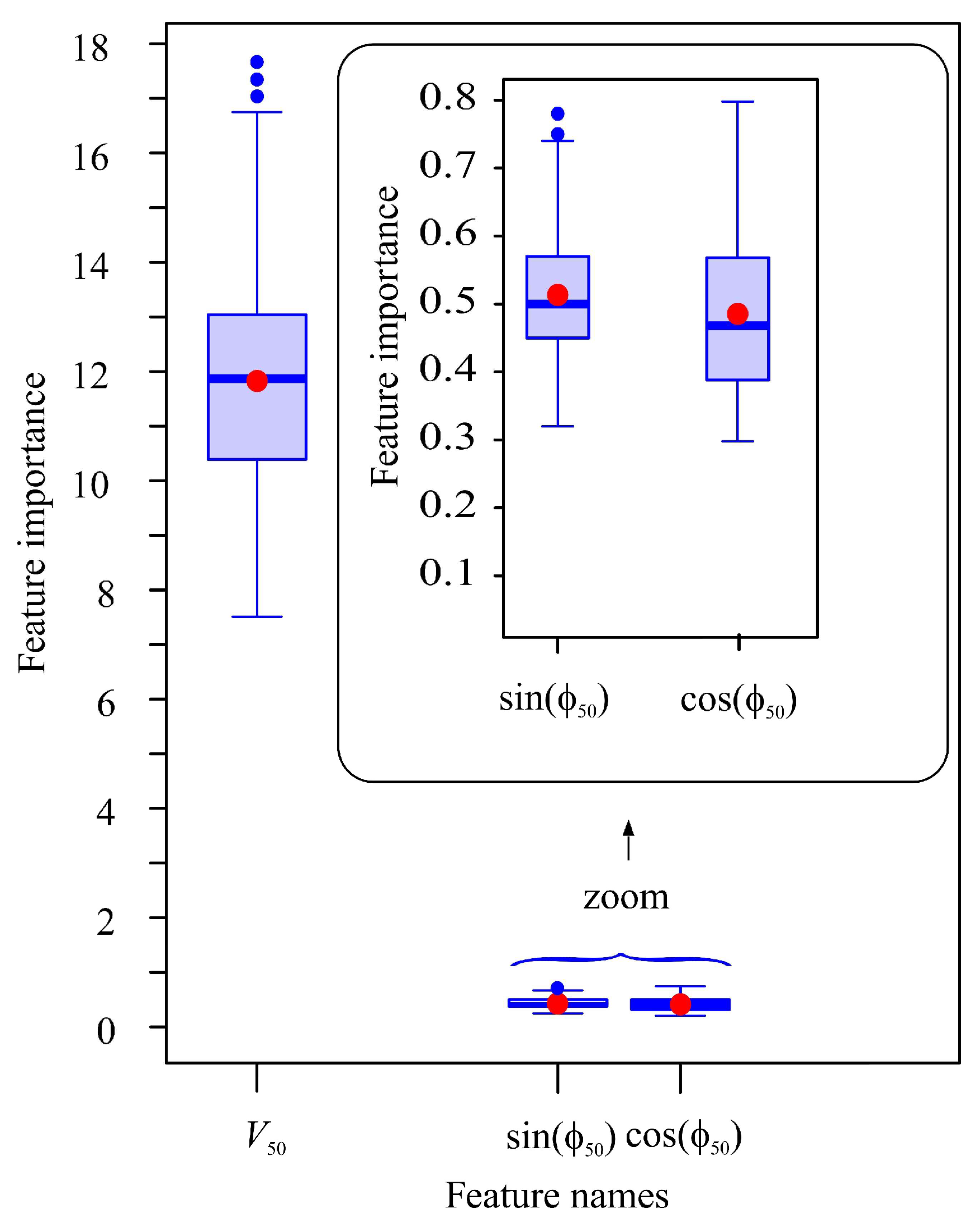
Appendix A.6. Permutation Importance of the Input Features of the RF Models

Figure A9 shows the permutation importance of the input features of the RF models.
Figure A9. Permutation importance of the input features of the RF models.
Jmse 13 01213 g0a9

Appendix A.7. Boxplot of the MAEs Obtained in the Tests Undertaken

Figure A10 shows the Boxplot of the MAEs obtained in the tests undertaken.
Figure A10. Boxplot of the MAEs obtained in the tests undertaken.
Jmse 13 01213 g0a10

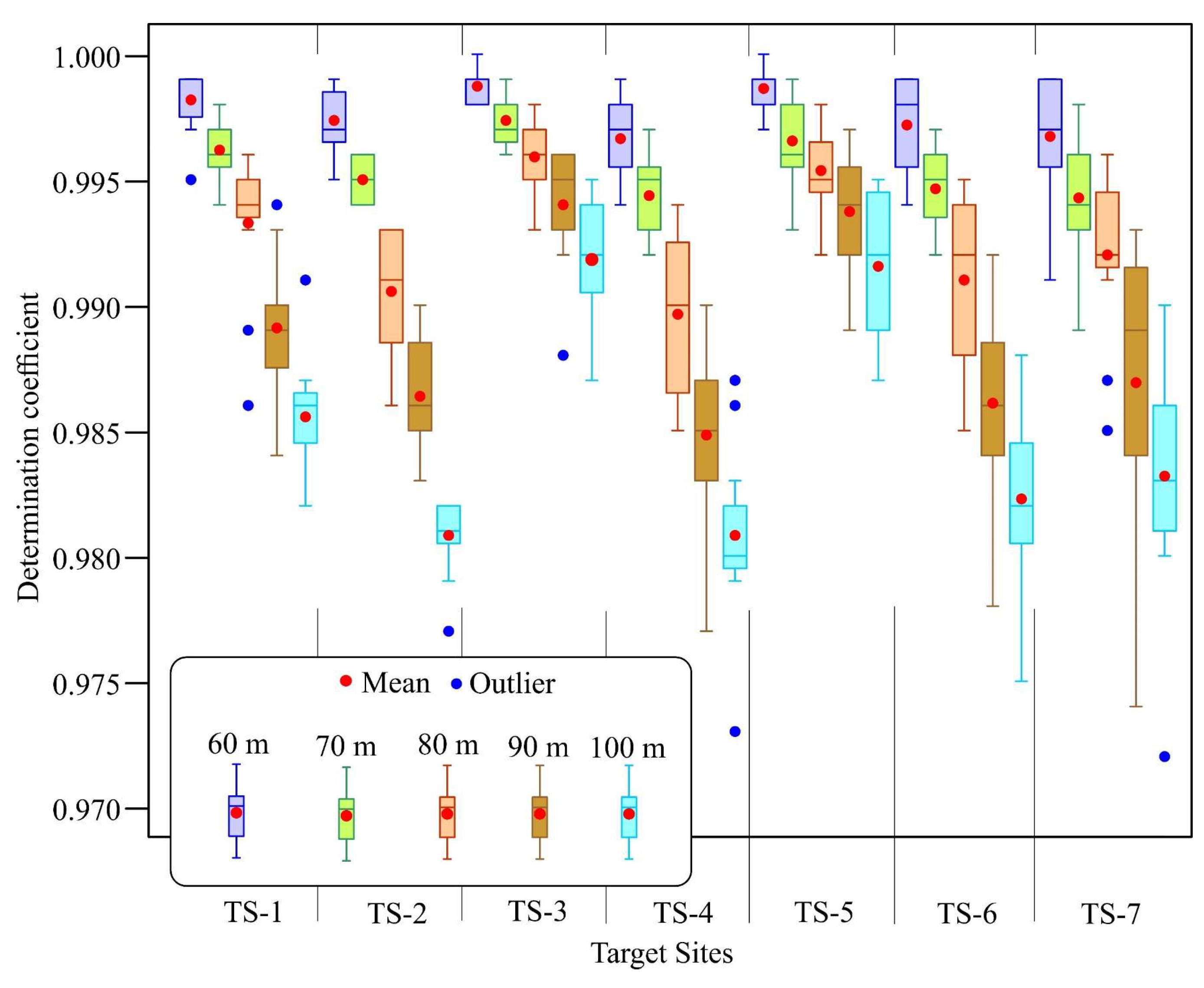
Appendix A.8. Boxplot of the R2 Metrics Obtained in the Tests Undertaken

Figure A11 shows boxplot of the R2 metrics obtained in the tests undertaken.
Figure A11. Boxplot of the R2 metrics obtained in the tests undertaken.
Jmse 13 01213 g0a11

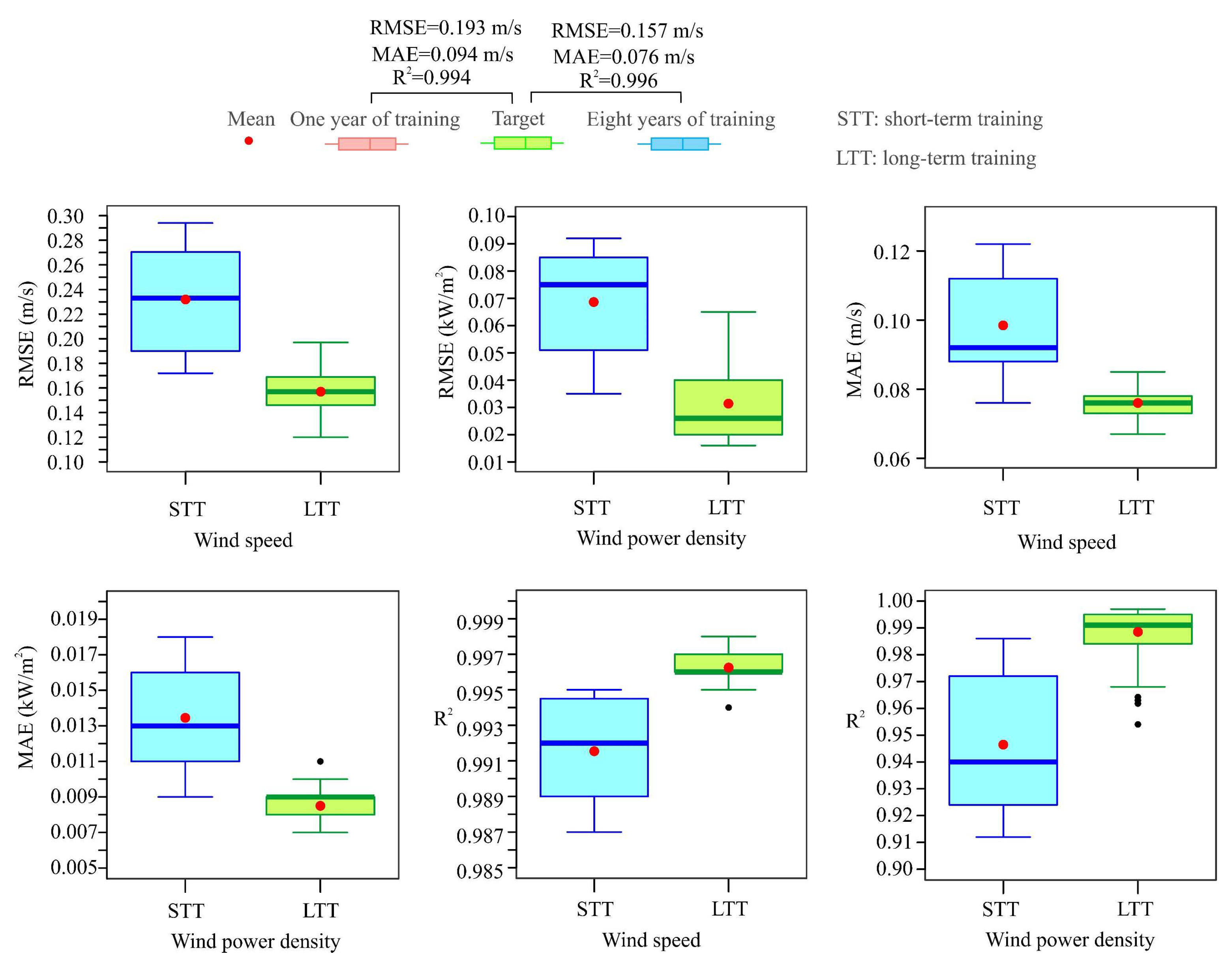
Appendix A.9. Boxplots of the Test Metrics of the RF Models Based on One Year and Eight Years of Training/Validation

Figure A12 shows boxplot of the test metrics of the RF models based on one year and eight years of training/validation.
Figure A12. Boxplots of the test metrics of the RF models based on one year and eight years of training/validation.
Jmse 13 01213 g0a12

References

  1. Cabrera, P.; Lund, H.; Carta, J.A. Smart renewable energy penetration strategies on islands: The case of Gran Canaria. Energy 2018, 162, 421–443. [Google Scholar] [CrossRef]
  2. Lund, H.; Thellufsen, J.Z.; Østergaard, P.A.; Sorknæs, P.; Skov, I.R.; Mathiesen, B.V. EnergyPLAN—Advanced analysis of smart energy systems. Smart Energy 2021, 1, 1000007. [Google Scholar] [CrossRef]
  3. Cabrera, P.; Lund, H.; Thellufsen, J.Z.; Sorknæs, P. The MATLAB Toolbox for EnergyPLAN: A tool to extend energy planning studies. Sci. Comput. Program. 2020, 191, 102405. [Google Scholar] [CrossRef]
  4. Yan, J.; Zhang, H.; Liu, Y.; Han, S.; Li, L. Uncertainty estimation for wind energy conversion by probabilistic wind turbine power curve modelling. Appl. Energy 2019, 239, 1356–1370. [Google Scholar] [CrossRef]
  5. Díaz, S.; Carta, J.A.; Matías, J.M. Comparison of several measure-correlate-predict models using support vector regression techniques to estimate wind power densities. A case study. Energy Convers. Manag. 2017, 140, 334–354. [Google Scholar] [CrossRef]
  6. Díaz, S.; Carta, J.A.; Matías, J.M. Performance assessment of five MCP models proposed for the estimation of long-term wind turbine power outputs at a target site using three machine learning techniques. Appl. Energy 2018, 209, 455–477. [Google Scholar] [CrossRef]
  7. Ahmad, M.; Zeeshan, M. Validation of weather reanalysis datasets and geospatial and techno-economic viability and potential assessment of concentrated solar power plants. Energy Convers. Manag. 2022, 256, 11536. [Google Scholar] [CrossRef]
  8. Liang, Y.; Wu, C.; Zhang, M.; Ji, X.; Shen, Y.; He, J.; Zhang, Z. Statistical modelling of the joint probability density function of air density and wind speed for wind resource assessment: A case study from China. Energy Convers. Manag. 2022, 268, 116054. [Google Scholar] [CrossRef]
  9. Yu, S.; Vautard, R. A transfer method to estimate hub-height wind speed from 10 meters wind speed based on machine learning. Renew. Sustain. Energy Rev. 2022, 169, 112897. [Google Scholar] [CrossRef]
  10. Crippa, P.; Alifa, M.; Bolster, D.; Genton, M.G.; Castruccio, S. A temporal model for vertical extrapolation of wind speed and wind energy assessment. Appl. Energy 2021, 301, 117378. [Google Scholar] [CrossRef]
  11. Mohandes, M.; Rehman, S.; Rahman, S. Estimation of wind speed profile using adaptive neuro-fuzzy inference system (ANFIS). Appl. Energy 2011, 88, 4024–4032. [Google Scholar] [CrossRef]
  12. Carta, J.A.; Velázquez, S.; Cabrera, P. A review of measure-correlate-predict (MCP) methods used to estimate long-term wind characteristics at a target site. Renew. Sustain. Energy Rev. 2013, 27, 362–400. [Google Scholar] [CrossRef]
  13. de Aquino Ferreira, S.C.; Oliveira, F.L.C.; Maçaira, P.M. Validation of the representativeness of wind speed time series obtained from reanalysis data for Brazilian territory. Energy 2022, 258, 124746. [Google Scholar] [CrossRef]
  14. Gelaro, R.; McCarty, W.; Suárez, M.J.; Todling, R.; Molod, A.; Takacs, L.; Randles, C.A.; Darmenov, A.; Bosilovich, M.G.; Reichle, R.; et al. The Modern-Era Retrospective Analysis for Research and Applications, Version 2 (MERRA-2). J. Clim. 2017, 30, 5419–5454. [Google Scholar] [CrossRef]
  15. Pelser, T.; Weinand, J.M.; Kuckertz, P.; McKenna, R.; Linssen, J.; Stolten, D. Reviewing accuracy & reproducibility of large-scale wind resource assessments. Adv. Appl. Energy 2024, 13, 100158. [Google Scholar] [CrossRef]
  16. Brower, M.C.; Bailey, B.H.; Beaucage, P.; Bernadett, D.W.; Doane, J.; Eberhard, M.J.; Elsholz, K.V.; Filippelli, M.V.; Hale, E.; Markus, M.J.; et al. Wind Resource Assessment: A Practical Guide to Developing a Wind Project; John Wiley & Sons, Inc.: Hoboken, NJ, USA, 2012. [Google Scholar] [CrossRef]
  17. Landberg, L. Meteorology for Wind Energy: An Introduction; John Wiley & Sons, Inc.: Hoboken, NJ, USA, 2015; pp. 1–204. [Google Scholar] [CrossRef]
  18. Zhang, M.H. Wind Resource Assessment and Micro-Siting; John Wiley & Sons: Hoboken, NJ, USA, 2015; pp. 1–293. [Google Scholar] [CrossRef]
  19. Watson, S. Handbook of Wind Resource Assessment; John Wiley & Sons: Hoboken, NJ, USA, 2023; pp. 1–297. [Google Scholar] [CrossRef]
  20. de Assis Tavares, L.F.; Shadman, M.; Assad, L.P.d.F.; Estefen, S.F. Influence of the WRF model and atmospheric reanalysis on the offshore wind resource potential and cost estimation: A case study for Rio de Janeiro State. Energy 2022, 240, 122767. [Google Scholar] [CrossRef]
  21. Gualtieri, G. A comprehensive review on wind resource extrapolation models applied in wind energy. Renew. Sustain. Energy Rev. 2019, 102, 215–233. [Google Scholar] [CrossRef]
  22. Gruber, K.; Klöckl, C.; Regner, P.; Baumgartner, J.; Schmidt, J. Assessing the Global Wind Atlas and local measurements for bias correction of wind power generation simulated from MERRA-2 in Brazil. Energy 2019, 189, 116212. [Google Scholar] [CrossRef]
  23. Prasad, A.A.; Taylor, R.A.; Kay, M. Assessment of solar and wind resource synergy in Australia. Appl. Energy 2017, 190, 354–367. [Google Scholar] [CrossRef]
  24. Yip, C.M.A.; Gunturu, U.B.; Stenchikov, G.L. Wind resource characterization in the Arabian Peninsula. Appl. Energy 2016, 164, 826–836. [Google Scholar] [CrossRef]
  25. Gunturu, U.B.; Schlosser, C.A. Characterization of wind power resource in the United States. Atmos. Meas. Tech. 2012, 12, 9687–9702. [Google Scholar] [CrossRef]
  26. Ritter, M.; Deckert, L. Site assessment, turbine selection, and local feed-in tariffs through the wind energy index. Appl. Energy 2017, 185, 1087–1099. [Google Scholar] [CrossRef]
  27. Ren, G.; Wan, J.; Liu, J.; Yu, D. Spatial and temporal assessments of complementarity for renewable energy resources in China. Energy 2019, 177, 262–275. [Google Scholar] [CrossRef]
  28. Ren, G.; Wan, J.; Liu, J.; Yu, D. Characterization of wind resource in China from a new perspective. Energy 2019, 167, 994–1010. [Google Scholar] [CrossRef]
  29. Gao, Y.; Ma, S.; Wang, T.; Wang, T.; Gong, Y.; Peng, F.; Tsunekawa, A. Assessing the wind energy potential of China in considering its variability/intermittency. Energy Convers. Manag. 2020, 226, 113580. [Google Scholar] [CrossRef]
  30. Logarithmic Profile for Wind Profile Program. (n.d.). Available online: http://www.met.reading.ac.uk/~marc/it/wind/interp/log_prof/ (accessed on 10 February 2023).
  31. Valsaraj, P.; Thumba, D.A.; Asokan, K.; Kumar, K.S. Symbolic regression-based improved method for wind speed extrapolation from lower to higher altitudes for wind energy applications. Appl. Energy 2020, 260, 114270. [Google Scholar] [CrossRef]
  32. Mohandes, M.A.; Rehman, S. Wind Speed Extrapolation Using Machine Learning Methods and LiDAR Measurements. IEEE Access 2018, 6, 77634–77642. [Google Scholar] [CrossRef]
  33. Nuha, H.; Mohandes, M.; Rehman, S.; A-Shaikhi, A. Vertical wind speed extrapolation using regularized extreme learning machine. FME Trans. 2022, 50, 412–421. [Google Scholar] [CrossRef]
  34. Islam, S.; Mohandes, M.; Rehman, S. Vertical extrapolation of wind speed using artificial neural network hybrid system. Neural Comput. Appl. 2016, 28, 2351–2361. [Google Scholar] [CrossRef]
  35. Al-Shaikhi, A.; Nuha, H.; Mohandes, M.; Rehman, S.; Adrian, M. Vertical wind speed extrapolation model using long short-term memory and particle swarm optimization. Energy Sci. Eng. 2022, 10, 4580–4594. [Google Scholar] [CrossRef]
  36. Al-Shaikhi, A.; Nuha, H.H.; Lawal, A.; Rehman, S.; Mohandes, M. Vertical Wind Profile Estimation Using Hybrid Convolutional Neural Networks and Bidirectional Long Short-Term Memory. Arab. J. Sci. Eng. 2023, 48, 6915–6924. [Google Scholar] [CrossRef]
  37. Rehman, S.; Nuha, H.H.; Al Shaikhi, A.; Akbar, S.; Mohandes, M. Improving Performance of Recurrent Neural Networks Using Simulated Annealing for Vertical Wind Speed Estimation. Energy Eng. 2023, 120, 775–789. [Google Scholar] [CrossRef]
  38. R Interface to NLopt, version 2.0.3; R package nloptr; The R Foundation: Vienna, Austria, 2022.
  39. Holtslag, M.C.; Bierbooms, W.A.A.M.; van Bussel, G.J.W. Estimating atmospheric stability from observations and correcting wind shear models accordingly. J. Phys. Conf. Ser. 2014, 012052. [Google Scholar] [CrossRef]
  40. Mpholo, M.; Mathaba, T.; Letuma, M. Wind profile assessment at Masitise and Sani in Lesotho for potential off-grid electricity generation. Energy Convers. Manag. 2012, 53, 118–127. [Google Scholar] [CrossRef]
  41. Dyer, A.J. A review of flux-profile relationships. Bound. Layer Meteorol. 1974, 7, 363–372. [Google Scholar] [CrossRef]
  42. Beljaars, A.C.M.; Holtslag, A.A.M. American Meteorological Society Flux Parameterization over Land Surfaces for Atmospheric Models. J. Appl. Meteorol. Climatol. 1988, 30, 327–341. [Google Scholar] [CrossRef]
  43. Paulson, C.A. The Mathematical Representation of Wind Speed and Temperature Profiles in the Unstable Atmospheric Surface Layer. J. Appl. Meteorol. 1970, 9, 857–861. [Google Scholar] [CrossRef]
  44. Grachev, A.A.; Fairall, C.W.; Bradley, E.F. Convective Profile Constants Revisited. Bound. Layer Meteorol. 2000, 94, 495–515. [Google Scholar] [CrossRef]
  45. Breiman, L. Random forests. Mach. Learn. 2001, 45, 5–32. [Google Scholar] [CrossRef]
  46. Carta, J.A.; Cabrera, P. Optimal sizing of stand-alone wind-powered seawater reverse osmosis plants without use of massive energy storage. Appl. Energy 2021, 304, 117888. [Google Scholar] [CrossRef]
  47. Optis, M.; Bodini, N.; Debnath, M.; Doubrawa, P. New methods to improve the vertical extrapolation of near-surface offshore wind speeds. Wind. Energy Sci. 2021, 6, 935–948. [Google Scholar] [CrossRef]
  48. Emeis, S. Wind Energy Meteorology: Atmospheric Physics for Wind Power Generation. Green Energy Technol. 2013, 99, 189–192. [Google Scholar] [CrossRef]
  49. Carta, J.A.; Cabrera, P.; Matías, J.M.; Castellano, F. Comparison of feature selection methods using ANNs in MCP-wind speed methods. A case study. Appl. Energy 2015, 158, 490–507. [Google Scholar] [CrossRef]
  50. randomForest: Breiman and Cutler’s Random Forests for Classification and Regression Version 4.6-10 from R-Forge. Available online: https://rdrr.io/rforge/randomForest/ (accessed on 20 February 2023).
  51. R: The R Project for Statistical Computing. Available online: https://www.R-project.org/ (accessed on 20 February 2023).
  52. Package “Tune” Title Tidy Tuning Tools, version 1.0.1; The R Foundation: Vienna, Austria, 2022.
  53. V-Fold Cross-Validation—Vfold_cv—rsample. Available online: https://rsample.tidymodels.org/reference/vfold_cv.html (accessed on 20 February 2023).
  54. Hatfield, D.; Hasager, C.B.; Karagali, I. Vertical extrapolation of ASCAT ocean surface winds using machine learning techniques. Wind Energy Sci. Discuss. 2022, 8, 1–26. [Google Scholar]
  55. Carta, J.; Ramírez, P.; Velázquez, S. A review of wind speed probability distributions used in wind energy analysis. Renew. Sustain. Energy Rev. 2009, 13, 933–955. [Google Scholar] [CrossRef]
  56. Chavan, D.S.; Gaikwad, S.; Singh, A.; Himanshu; Parashar, D.; Saahil, V.; Sankpal, J.; Karandikar, P.B. Impact of vertical wind shear on wind turbine performance. In Proceedings of the IEEE International Conference on Circuit, Power and Computing Technologies (ICCPCT 2017), Kollam, India, 20–21 April 2017; Institute of Electrical and Electronics Engineers Inc.: Piscataway, NJ, USA, 2017. [Google Scholar] [CrossRef]
  57. Taylor, M.; Mackiewicz, P.; Brower, M.C.; Markus, M. An analysis of wind resource uncertainty in energy production estimates. In Proceedings of the European Wind Energy Conference & Exhibition, London, UK, 22–25 November 2004; pp. 951–952. [Google Scholar]
  58. Miguel, J.V.P.; Fadigas, E.A.; Sauer, I.L. The Influence of the Wind Measurement Campaign Duration on a Measure-Correlate-Predict (MCP)-Based Wind Resource Assessment. Energies 2019, 12, 3606. [Google Scholar] [CrossRef]
  59. ENERCON Product Porfolio. Available online: https://portal.ct.gov/-/media/csc/1_dockets-medialibrary/petition_983/dm_plan/2020_0109_dandm_modification/exhibitaenerconturbinesbrochuree138ep3pdf.pdf?rev=b0d2297308b3476fab665df83d8d952c&hash=B1EBFE98A964A8BA9D5A98BB6258828A (accessed on 27 May 2025).
  60. Tümse, S.; İlhan, A.; Bilgili, M.; Şahin, B. Estimation of wind turbine output power using soft computing models. Energy Sources Part A Recover. Util. Environ. Eff. 2022, 44, 3757–3786. [Google Scholar] [CrossRef]
  61. Prasad, K.M.; Nagababu, G.; Jani, H.K. Enhancing offshore wind resource assessment with LIDAR-validated reanalysis datasets: A case study in Gujarat, India. Int. J. Thermofluids 2023, 18, 100320. [Google Scholar] [CrossRef]
Figure 1. Schematic representation of the process used for extrapolating hourly mean wind speeds from the MERRA2 reanalysis to wind turbine hub heights.
Jmse 13 01213 g001
Figure 2. Schematic representation of the first task of the method employed.
Jmse 13 01213 g002
Figure 3. Schematic representation of the second task of the method employed.
Jmse 13 01213 g003
Figure 4. Location of the case study.
Jmse 13 01213 g004
Figure 5. Boxplot of the monthly mean wind speeds at 2 m, 10 m, and 50 m above ground level at the target sites during the 11 years considered (2011–2021).
Jmse 13 01213 g005
Figure 6. Relative frequencies of best fit of the 21 models analyzed.
Jmse 13 01213 g006
Figure 7. Comparison of APDs obtained at 100 m height between the best models and the other models analyzed, for the seven TSs of the case study.
Jmse 13 01213 g007
Figure 8. Example of models used in TS-1, in each time step, when estimating wind speeds at 100 m height. Dates: 23 and 24 February 2020.
Jmse 13 01213 g008
Figure 9. Boxplot of the RMSEs obtained in the validation and testing of the models at the different target sites (TSs) and at different heights.
Jmse 13 01213 g009
Figure 10. Validation and test boxplot of TS-5 at 100 m height.
Jmse 13 01213 g010
Figure 11. Comparison of the mean hourly power output that the ENERCON E-70 wind turbine (2300 kW rated power) would have generated with mean hourly TS-5 target wind speed at 100 m height (red) for 700 h in 2015, RF eight-year wind speed (blue), and RF one-year wind speed (green).
Jmse 13 01213 g011
Table 2. The surface layer wind speed profile. Empirical stability function y(h/L). L is the Obukhov length.
Numbery(h/L)Reference
15 ψ h L = 5 h L [41]
16 ψ h L = h L 2 3 h L 5 0.35 exp 0.35 h L 10 1.05 [42]
17 and 20 ψ h L = 0 [19]
18 ψ h L = 2 L n 1 + X 2 + ln 1 + X 2 2 2 arctan X + π 2 [43]
X = ( 1 16 h L ) 1 / 4
19 ψ h L = 3 2 Ln y 2 + y + 1 3 3 arctan 2 y + 1 3 + π 3 y = ( 1 10 h L ) 1 / 3 [44]
Disclaimer/Publisher’s Note: The statements, opinions and data contained in all publications are solely those of the individual author(s) and contributor(s) and not of MDPI and/or the editor(s). MDPI and/or the editor(s) disclaim responsibility for any injury to people or property resulting from any ideas, methods, instructions or products referred to in the content.

