Impacts of Wind Assimilation on Error Correction of Forecasted Dynamic Loads from Wind, Wave, and Current for Offshore Wind Turbines

Abstract

In this study, a dynamic load forecasting model was developed for offshore wind turbines, based on the COAWST (Coupled Ocean-Atmosphere-Wave-Sediment Transport) model, the GRU (Gated Recurrent Unit) algorithm, and a data assimilation module. The model was able to forecast aerodynamic, wave, and current loads acting on the turbines. Four groups of forecasting tests were conducted to evaluate the model’s performance under different strategies and to assess the impact of atmospheric assimilation on improving dynamic load forecasts. The wind turbines in Cangnan Offshore Wind Farm, located in the west of the East China Sea, were chosen as the study object. The results indicated that the model achieved high forecasting accuracy, with the RMSEs (root mean square errors) of 275.59 kN, 335.85 kN, and 313.51 N, for the aerodynamic, wave, and current loads. The errors were reduced by about 13%, 10.09%, and 6.7% when compared with the original COAWST model, and were also lower than the atmospheric and oceanic reanalysis data. Atmospheric data assimilation was demonstrated to reduce the forecasting RMSE of aerodynamic load by about 12%, and its error improvement was able to be combined with GRU-based error correction. Additionally, atmospheric assimilation mitigated the reduction in temporal variability caused by forecasting error correction, preventing a decrease in the standard deviation of aerodynamic load forecasts. However, atmospheric assimilation had minimal impacts on wave and current load forecasts, with the RMSEs increased by about 2.5% and 0.1%, and had almost the same performance in correlation coefficients and standard deviations.

1. Introduction

Wind energy is widely recognized as one of the most promising sources of renewable energy [1]. According to the Global Wind Energy Report by the Global Wind Energy Council (available online at https://www.gwec.net/reports/globalwindreport/2024, accessed on 19 June 2025), a record 117 GW of new wind energy capacity was installed worldwide in 2023, representing a 50% increase compared to 2022. Offshore wind power is growing particularly rapidly, owing to fewer environmental and noise concerns compared to onshore wind power. Additionally, wind speed generally increases with distance from the shore, resulting in higher energy generation [2].

Most offshore wind turbines are typically installed on concrete-piled foundations anchored to the seabed. Under these conditions, wind turbines are subjected to stresses from multiple factors, including soil, currents, waves, and wind [3]. Unlike soil stresses, which change gradually, dynamic loads from the ocean and atmosphere fluctuate in real time. During long-term operation, wind turbine structures are exposed to fluctuating dynamic loads, leading to increased structural fatigue and a higher risk of damage [4].

In extreme environments (e.g., strong winds and large waves), the risk of structural damage to wind turbines increases considerably [5]. For instance, in 2003, Typhoon Dujuan struck the Honghai Bay wind farm, damaging the blades of nine turbines and destroying the control systems of six. This occurred despite the fact that the typhoon’s wind speed was much lower than the design-level extreme wind speed [6]. In 2013, Typhoon Usagi struck a wind farm on an island off the east coast of Shanwei City, causing rotor blade damage, tower collapse, and even turbine combustion [7]. On 8 August 2015, Typhoon Soudelor made landfall in Taiwan, fracturing the blades of one wind turbine and toppling six turbine towers [8].

These accidents were engineering failures induced by extreme weather, leading to substantial economic losses. However, the structural strength of wind turbines cannot be infinitely increased during manufacturing and construction. Therefore, accurate prediction and assessment of dynamic loads on offshore wind turbines serve as crucial references for engineering design and construction, playing a critical role in ensuring the stability and safety of offshore wind power systems.

The dynamic load on a wind turbine is influenced by both the turbine’s geometry and environmental factors. According to previous studies [9,10,11,12,13,14], the dynamic loads acting on wind turbines from air and seawater can be divided into two main categories. Loads from the air are generally called aerodynamic loads, which are typically divided into blade wind loads and tower loads for separate calculation. The primary environmental factor affecting aerodynamic loads is the wind speed profile. Loads from seawater are typically categorized as wave loads and current loads, influenced by wave speed and current speed, respectively. Thus, variations in dynamic loads depend on the accurate prediction of three key factors: wind speed, wave speed, and current speed.

Extensive efforts have been made to improve the forecasting accuracy of ocean dynamic environments, aiming to obtain more accurate predictions of wind, wave, and current conditions. Among these efforts, numerical prediction methods are the most commonly employed. Researchers generate conventional forecasts using numerical models and improve the accuracy of initial and boundary conditions by incorporating observational data through data assimilation techniques. For instance, in wind speed forecasting, Rana et al. enhanced numerical predictions by using wind speed inversion data near the Wadden Sea in Western Europe. Compared to the ECMWF (European Centre for Medium-Range Weather Forecasts) forecast product, the RMSE (root mean square error) was reduced by 42.4% [15]. Cassola et al. combined a Kalman filter assimilation method with a numerical weather model to forecast both wind speed and wind energy. The MAE (mean absolute error) of the assimilated wind speed forecast was reduced by approximately 25% for short-term forecasts and by about 10% for near-term wind speed predictions [16]. Mirouze et al. assimilated satellite surface current velocity observations into the MOI (Mercator Ocean International) system. In simulations of the tropical Atlantic Ocean, Gulf Stream, and Equatorial Current, the RMSE of surface current forecasts was reduced when compared to the NR (Nature Run) model, with greater improvements observed in tropical regions [17]. Rusu developed a numerical wave prediction system for the Black Sea using the SWAN (Simulating Waves Nearshore) model, combined with a Kalman filter assimilation method. Historical hindcast tests demonstrated that data assimilation significantly improved the accuracy of numerical wave forecasts [18].

In addition to conventional numerical forecasting, data-driven empirical forecasting methods have developed rapidly in recent years. These empirical forecasting methods establish mapping models between historical data and future changes through data mining. The most commonly used empirical forecasting methods can generally be divided into two categories. The first category includes traditional mathematical statistical methods, both linear and nonlinear. For instance, Kavasseri et al. used the fractional ARIMA (Auto Regressive Integrated Moving Average) method to forecast wind speed in North Dakota, USA, for 24 h and 48 h. Compared with other methods, the RMSE was reduced by 42% [19]. The second category consists of artificial intelligence forecasting methods based on machine learning or deep learning [20]. With the advancements in artificial intelligence, the accuracy of these models continues to improve, making them an important development direction for future meteorological and hydrological forecasting. For example, Zhou et al. employed the LS-SVM (Least Squares-Support Vector Machine) method to forecast short-term wind speed in North Dakota, USA, and compared it with persistence models. They found that the RMSE of wind speed was reduced by 38% [21]. Özger applied the WFL (Wavelet Transform Fuzzy Logic) method to forecast significant wave height on the U.S. west coast, and compared it with other models, such as ARMA (Auto Regressive Moving Average), ANN (Artificial Neural Network), and FL (Fuzzy Logic). The results showed that the WFL model was particularly superior in long-term forecasting [22]. Liu et al. introduced an exponential function-based step size and elite reverse learning strategy in the MODA (Multi-Objective Dragonfly Algorithm), developing the ICEEMDAN-MMODA model, and used it for short-term wind speed forecasting on the Shandong Peninsula. Comparative studies with various classical single models and optimized algorithm models demonstrated that this model not only offered high efficiency and low cost but also significantly improved forecasting accuracy [23]. Halicki et al. employed AR (Autoregressive Model), ARIMA, and LSTM (Long-Short Term Memory) models for short-term wave forecasting in the Baltic Sea. The study found that the LSTM model exhibited outstanding prediction accuracy over longer time periods, further validating the advantages of neural networks in effective wave height forecasting. Additionally, the research demonstrated that proper adjustments, such as optimization, regularization, and validation, could achieve better results in wave forecasting [24]. However, it is undeniable that due to the lack of physical mechanism constraints and interpretability, these empirical methods still face significant challenges in short-term forecasting within seven days.

In recent years, error correction based on numerical forecasting results has gained widespread attention with the rise in artificial intelligence. This method establishes error correction models for numerical models using artificial intelligence algorithms to eliminate forecasting errors. This approach combines the advantages of both numerical dynamic simulations and empirical algorithms [25]. Compared to purely empirical forecasting models, it provides more stable results under physical mechanism constraints, reducing the likelihood of unreasonable outcomes. For example, Han et al. developed the WRF-PCC-CEEMDAN-CNN-BLSTM-AMGS model, which integrated the WRF (Weather Research and Forecasting) model with a novel hybrid deep learning algorithm. This model was used to correct wind speed forecasts in Colorado, with the MAE, MAPE (Mean Absolute Percentage Error), and RMSE decreasing by 94.13%, 91.75%, and 93.93%, respectively, compared to the uncorrected forecasts [26]. Frnda et al. used neural networks for error correction on two basic meteorological parameters from the ECMWF global forecast product, namely surface temperature and 24 h accumulated precipitation, in the Czech Republic and Slovakia. The verification results showed that the corrected errors (RMSE) were reduced by 13% (surface temperature) and 45% (24 h precipitation) [27]. Yang et al. applied the UNet model to correct wind speed forecast biases from the ECMWF High Resolution Model (HRES) in the East China region. The results indicated that the corrected wind speed forecasts improved by an average of 22.8% compared to the original forecasts [28].

While the above error correction studies have achieved effective results, many issues remain to be addressed. During the development of error correction models, we observed that the level of original forecasting errors is related to the effectiveness of error correction. Since correction models are prone to learning spurious relationships in the data, it becomes particularly challenging to build accurate correction models when the original errors are large [29]. Given that data assimilation can reduce forecasting errors by incorporating observational data, how would the introduction of data assimilation into the modeling process of empirical error correction models affect the correction of forecast errors? Would differences in assimilated data lead to variations in the correction results? Past studies have attempted to integrate data assimilation with deep learning or machine learning algorithms to enhance the prediction capabilities of environmental factors. For instance, Bourgin et al. studied the impact of data assimilation and model post-processing methods on hydrological ensemble forecasting. The study found that both methods significantly influenced the reliability of predictions, and the two strategies exhibited complementary effects [30]. Ham et al. developed a deep learning-based global ocean assimilation system, DeepDA, by integrating partial convolutional neural networks and generative adversarial networks. Using ocean assimilation data for observational system simulation experiments, the results showed that DeepDA significantly reduced the analysis errors of ocean temperature, with the RMSE of three-dimensional temperature analysis data decreasing by 40% [31].

The Cangnan Offshore Wind Farm is located along the coast of Wenzhou in Zhejiang Province, China. Construction of the project began in 2018, with plans to install 77 units of 5.2 MW offshore wind turbines. Supporting infrastructure includes a 220 kV offshore booster station and an onshore centralized control center, bringing the total installed capacity to 400 MW. Situated in the nearshore area of the East China Sea, the wind farm is vulnerable to extreme weather events, such as typhoons. Accurately predicting the dynamic load on the turbines can significantly enhance the wind farm’s safety and reliability.

Previously, we developed a forecasting system based on the COAWST (Coupled Ocean-Atmosphere-Wave-Sediment Transport) model, with good simulation capabilities for surface wind, waves, and other environmental factors. This study will build upon that system, integrating a three-dimensional ensemble variational assimilation model and the GRU error post-processing algorithm to establish a forecasting model for turbine dynamic loads. By constructing multiple sensitivity experiments and comparing the results of forecasts with and without assimilation, we aim to explore the impacts of the assimilation process on corrected forecasts and to investigate the changes in forecasting accuracy under different correction strategies.

2. Model and Data

2.1. Dynamic Load Forecasting Model for Wind Turbines

The dynamic load forecasting system developed in this study consists of the COAWST model, assimilation module, error correction module, and load calculation module.

2.1.1. COAWST Model

The COAWST model, developed by Warner et al. in 2010 [32], is a coupled model composed of several components: the WRF, ROMS (Regional Ocean Modeling System), and SWAN models. The MCT (Model Coupling Toolkit) is used to decompose each component model into segments, with processors assigned to each segment. The parallel coupling method then facilitates the transmission and conversion of various distributed data among the components [32].

Previous studies have shown that the COAWST model demonstrates excellent performance. For example, Liu et al. used the COAWST model to simulate Typhoon Muifa in 2011. The results indicated that the COAWST model was able to accurately simulate the oceanic and atmospheric processes during the typhoon [33]. Thankaswamy et al. used the COAWST model to simulate the development of Typhoons Mujigae, Merbok, and Hato. They found that the deviation in the typhoon’s trajectory, compared to the JTWC (Joint Typhoon Warning Center) report, was reduced by 10% to 40%, demonstrating the model’s good forecasting ability for intense typhoons [34].

2.1.2. Data Assimilation Module

This study utilized the 3D EnVar (three-dimensional ensemble variational assimilation) module in the WRF assimilation system to integrate radiosonde observation data into the COAWST simulation, thereby constraining the model’s initial and boundary fields. The 3D EnVar combines the static covariance in the cost function of 3DVAR (three-dimensional variational assimilation) with the background error covariance matrix, which changes with flow dynamics, in the ensemble Kalman filter method. Ensemble perturbations are added before the simulation each time to dynamically update the static covariance. Compared to the 3DVAR algorithm, which uses a static background error covariance matrix, the 3D EnVar algorithm is more adaptable to the rapid changes in weather conditions. Numerous studies have shown that this method outperforms three-dimensional variational assimilation in terms of forecast accuracy for meteorological elements [35,36,37].

2.1.3. Bias Correction Algorithm

In this study, the GRU algorithm was employed to correct the forecasting errors. The GRU algorithm captures dependencies across different time scales adaptively, enabling each recurrent unit to handle sequential data more effectively. Similarly to the LSTM algorithm, GRU includes gating units to regulate the flow of information within the unit. However, GRU does not have a separate memory cell, simplifying its structure [38]. Using historical observation data and continuous hindcast simulations of COAWST, a dataset for wind speed, current speed, and wave speed forecast errors was constructed for the training of the GRU neural network. After training, the GRU error correction module was coupled online with the COAWST model, and ultimately outputted the corrected forecasts for wind speed, current speed, and wave speed.

2.1.4. Dynamic Load Calculation Module

Wind turbines standing on seabed bedrock foundations are subjected to the combined forces of air, waves, water currents, and soil. In this study, soil stress calculation was not included. The other loads acting on the turbine include aerodynamic loads (separately calculated for blade wind loads and tower loads), wave loads, and current loads. The specific calculation methods are as follows:

(a)

Aerodynamic Loads

The aerodynamic loads on offshore wind turbines are divided into blade wind loads and tower loads. The blade wind loads can be calculated using the simplified formula as follows [39]:

$$F_a={\displaystyle \frac{1}{2}}{\rho }_a{A}_R{C}_T{U}^2$$

(1)

Here, $F_a$ represents the turbine load, ${\rho }_a$ is the air density, ${\rho }_a=1.255\mathrm{kg}/{\mathrm{m}}^3$. $A_R$ is the swept area of the rotor, calculated based on the blade size, $C_T$ is the thrust coefficient, and $U$ is the wind speed. Considering different wind speed ranges, the thrust coefficient can be obtained under three scenarios:

When the cut-in wind speed ($U_{in}$) ≤ wind speed ($U$) ≤ rated wind speed ($U_R$), the thrust coefficient is calculated using the following formula:

$$C_T={\displaystyle \frac{3.5\left(2U_R+3.5\right)}{U_R^2}}$$

(2)

When the rated wind speed ($U_R$) ≤ wind speed ($U$) ≤ cut-out wind speed ($U_{\mathrm{out}}$), the thrust coefficient is calculated using the following formula:

$$C_T=3.5U_R\left(2U_R+3.5\right)\cdot {\displaystyle \frac{1}{U^3}}$$

(3)

When operating under low wind speed conditions, it is assumed that the rotor thrust coefficient does not exceed 1. As a result, Equation (2) would overestimate the thrust coefficient, so its value is limited to 1.

The calculation formula for tower wind load is as follows [40]:

$$F_t={\displaystyle \frac{1}{2}}{\rho }_a{U}^2(Z)C_{\mathrm{d}}D$$

(4)

Here, $F_t$ represents the tower wind load, $C_{\mathrm{d}}$ is the drag coefficient, which is only related to the shape of the structure. In engineering, it is used to represent the resistance characteristics of an object in motion. For a tower with a cylindrical cross-section, $C_{\mathrm{d}}$ is typically taken as 0.5 after calculation. $D$ is the diameter of the monopile, and $U(Z)$ is the average wind speed at height $Z$.

(b)

Wave Loads

The wave load is simplified using the Morison equation [41], with the calculation formula as follows:

$$F_W={\displaystyle \frac{1}{2}}{C}_D{\rho }_s{A{U}_w}^2+C_M\rho V_0{U}_w$$

(5)

Here, $F_W$ represents the wave load, $A$ is the projected area of the unit cylindrical height perpendicular to the direction of wave propagation, $V_0$ is the displacement volume of the unit cylindrical height, ${\rho }_s$ is the seawater density, here ${\rho }_s=1025\mathrm{k}\mathrm{g}/{\mathrm{m}}^3$. $C_D$ is the drag coefficient in the direction perpendicular to the cylinder axis, $C_M$ is the inertia coefficient, and $U_w$ is the wave velocity. According to the industry standard “Hydrographic Specifications for Ports and Waterways” (JTS145-2015) [42], the $C_D$ and $C_M$ are set as 1.2 and 2.0 for cylinders under the influence of wave and current loads.

(c)

Current Loads

According to the industry standard “Code for Design of Wind Turbine Foundations for Offshore Wind Power Projects” (NB/T10105-2018) [43], the calculation method for current load is as follows:

$$F_C={\displaystyle \frac{1}{2}}{C}_W{\rho }_s{A{U}_c}^2$$

(6)

Here, $F_C$ represents the current load, $C_W$ is the drag coefficient, which is 0.73 for circular components, $A$ is the projected area, as previously explained, and $U_c$ is the current speed.

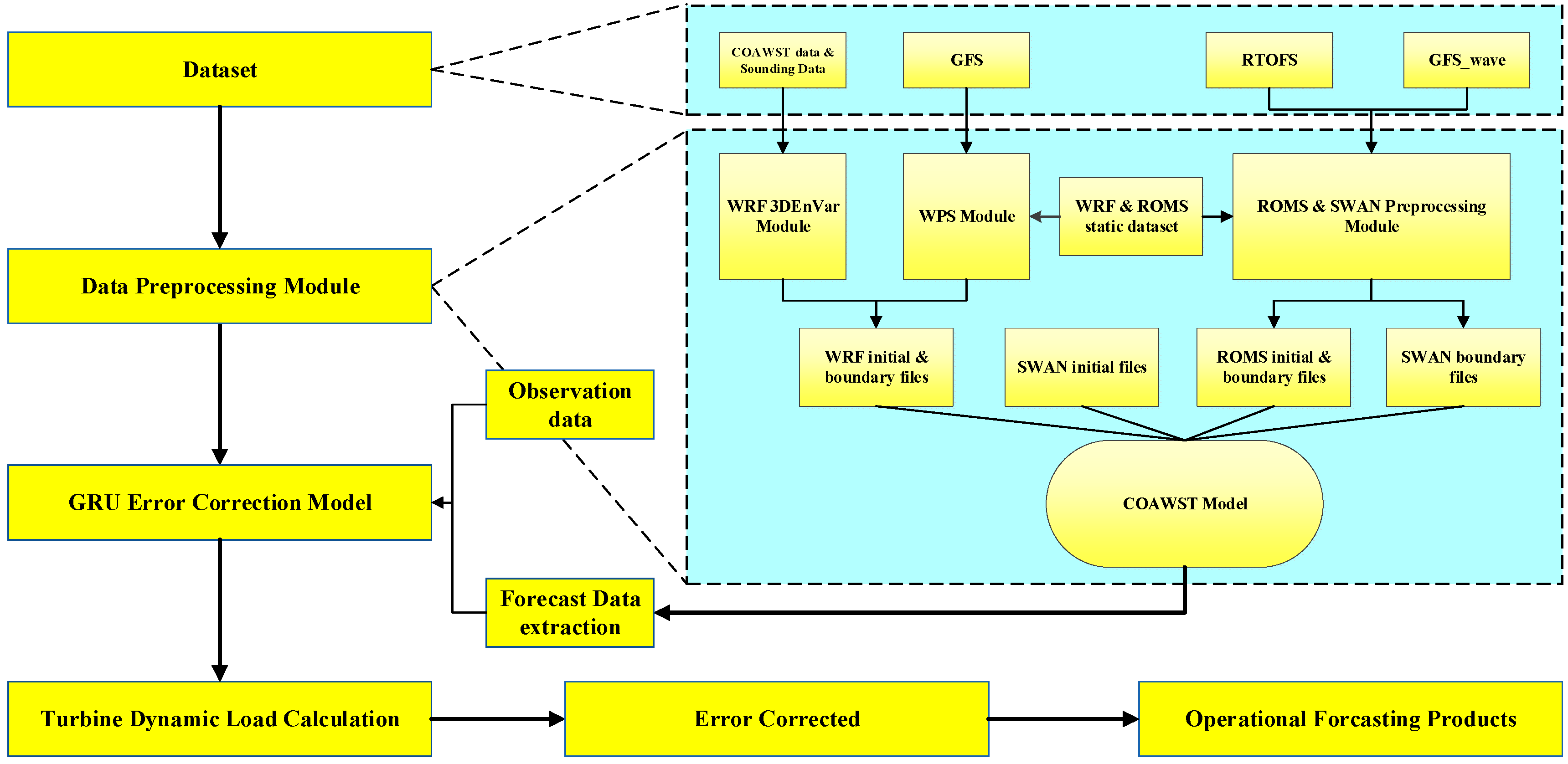
2.1.5. Flowchart of the Forecasting System

Figure 1 shows the flowchart of the forecasting system. First, a one-month continuous simulation was performed using the COAWST model, and the resulting data was used as a sample to calculate the static background covariance matrix. Next, radiosonde observation data was input into the data assimilation system, and observations of wind speed were assimilated at 00:00 UTC. These data were used as the observational input. Then, 10 ensemble samples were generated for the three-dimensional environment under the random CV scheme. The generated files were subsequently used as input for the minimization process of the 3D ensemble system. Finally, the analysis field files were updated to replace the initial and boundary field files of the COAWST model. The updated COAWST model input data drove the simulation, generating forecast results for the next 48 h. We extracted forecast variables such as wind speed, wave speed, and current speed, and used the GRU network for error correction training, ultimately outputting the corrected forecast results for wind speed, wave speed, and current speed. These corrected forecast results were then used for the corresponding load calculations.

2.2. Data Description

This study used wind, wave, and current observational data from the Cangnan Offshore Wind Farm to train and validate the forecast error correction module.

The Cangnan wind farm uses wind turbines supplied by Envision Technology Group, each with a rated capacity of 5.2 MW. The rotor diameter is 161 m, with a cut-in wind speed of 3.0 m/s, a cut-out wind speed of 25.0 m/s, and a rated wind speed of 10.7 m/s. All turbines are offshore and installed on piles anchored to the seabed. Tower heights vary, with the tallest tower reaching 230 m above mean sea level. The distance from the sea surface to the pile base is approximately 35 m. The turbines are designed to withstand a maximum horizontal load of 2811.1 kN [44,45].

The vertical wind data was obtained from wind sensors installed at various heights on the wind turbine towers. Wave observations were made using wave sensors on a sea surface buoy, and current measurements were taken from current meters on a subsurface buoy at different depths. The wind observation data consists of 19 height levels: 10 m, 50 m, 60 m, 70 m, 80 m, 90 m, 100 m, 110 m, 120 m, 130 m, 140 m, 150 m, 160 m, 170 m, 180 m, 190 m, 200 m, 210 m, and 230 m. The current observation data includes 7 depth levels: 4 m, 6 m, 12 m, 18 m, 24 m, 28 m, and 32 m. The raw observational data was quality-controlled according to the national standard “The Specification for Marine Observation—Part 6: Data Processing and Quality Control of Marine Observational Data” (GB/T14914.6-2021) [46]. During the data processing, values deviating more than three standard deviations from the mean were removed as anomalous. Missing data were filled using linear interpolation to ensure data continuity. All data were processed to a half-hour interval to match the time resolution of the model outputs.

The wind measurement data from the wind farm, together with surrounding radiosonde observation data, were incorporated into the data assimilation process. The radiosonde stations used for assimilation include Hangzhou, Hongjia, Fuzhou, Xiamen, and Quxian stations (site locations are shown in Figure 2). The radiosonde data was sourced from the University of Wyoming’s sounding data platform, with an observation frequency of every 12 h.

ERA5 (ECMWF Reanalysis v5) and CMEMS (Copernicus Marine Environment Monitoring Service) atmospheric and oceanic reanalysis data were also used in the evaluation of wind speed, current speed, and wave speed. ERA5 is the fifth generation of atmospheric reanalysis data produced by the European Centre for Medium-Range Weather Forecasts (ECMWF), with a spatial resolution of 0.25° × 0.25°. CMEMS data, provided by the EU Copernicus program, currently includes ocean physical data (temperature, salinity, sea level, currents), sea ice data (concentration, thickness, drift), and biogeochemical data (chlorophyll a, oxygen, pH, nutrients). The resolution of the data products is 1/12° for global scales [47]. Both datasets are frequently used as benchmark data for climate diagnostics and model comparisons.

3. Experimental Design

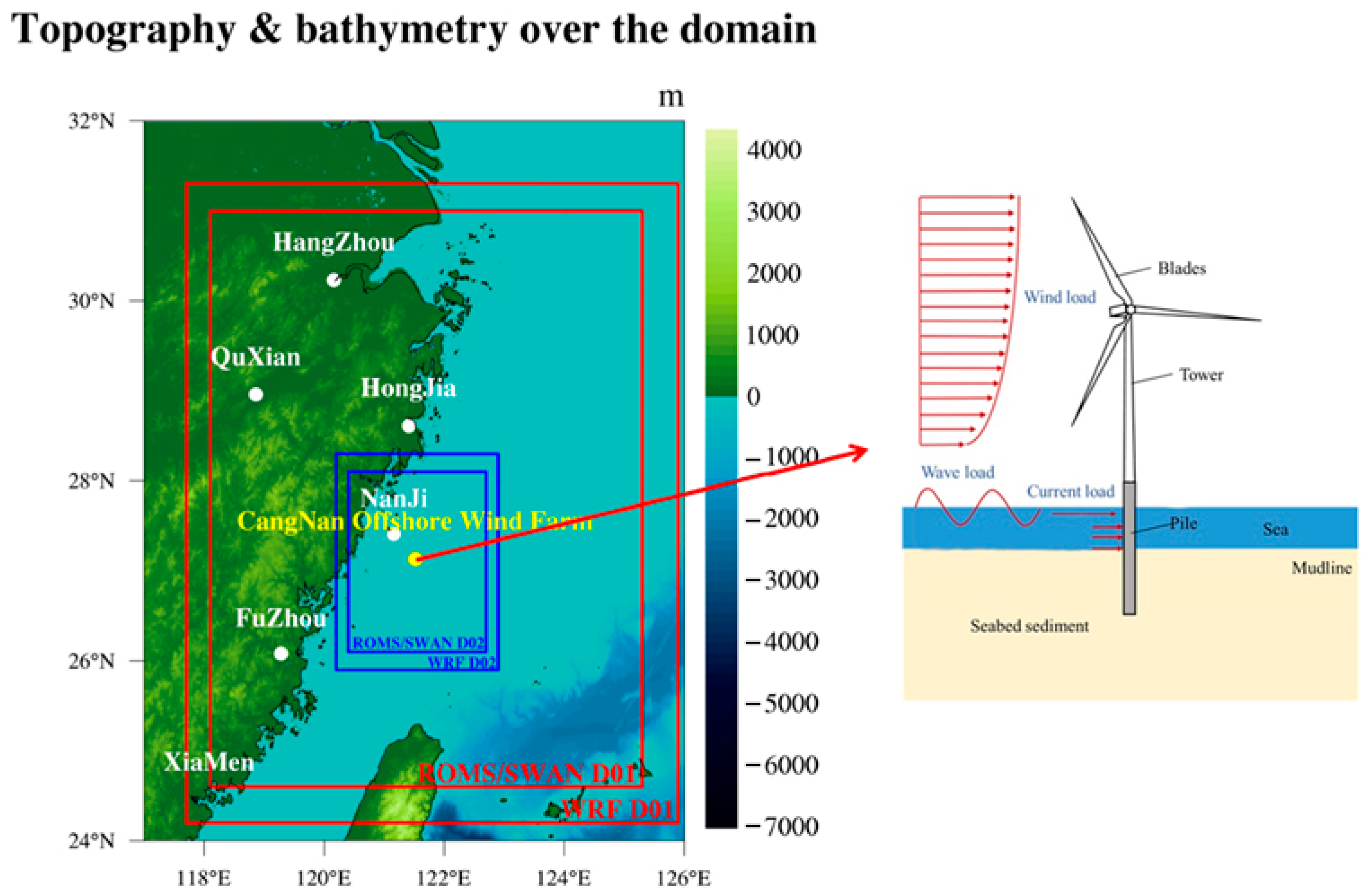
3.1. Model Configuration

In this study, the research domain is the region surrounding Cangnan Offshore Wind Farm, as shown in Figure 2.

The model configuration of COAWST is listed in

Table 1. Model configurations for the sub-models in the COAWST.

	WRF	ROMS	SWAN
Time Step	30 s	60 s	180 s
Gird Nesting	YES	YES	YES
Outer Grid Number	100 × 100	97 × 97	97 × 97
Inner Grid Number	100 × 100	97 × 97	97 × 97
Horizontal Grid Resolution	9 km for outer grid, 3 km for inner grid	9 km for outer grid, 3 km for inner grid	9 km for outer grid, 3 km for inner grid
Vertical Layer Number	51	16	None
Initial Data Source	GFS	RTOFS	GFS_wave
Variable Exchange Frequency	1800 s−1	1800 s−1	1800 s−1

.

The primary parameterization schemes for WRF included the WSM6 (WRF Single-Moment 6-Class) cloud microphysics scheme, the RRTM (Rapid Radiative Transfer Model) longwave radiation scheme, the Noah Land Surface Model for surface processes, and the GF (Grell-Freitas) cumulus convection parameterization scheme. For the ROMS setup, the Mellor-Yamada scheme was used to calculate turbulent mixing in the vertical direction, and the Flather boundary condition method was applied to calculate anisotropic currents, allowing the free propagation of wind-generated currents and tidal effects.

The WRF driving data was derived from the GFS (Global Forecast System, available online at https://www.ncei.noaa.gov/products/weather-climate-models/global-forecast, accessed on 19 June 2025), the ROMS driving data came from the RTOFS (Real-Time Ocean Forecast System, available online at https://www.nco.ncep.noaa.gov/pmb/products/rtofs/, accessed on 19 June 2025), and the SWAN driving data is sourced from GFS_wave. For model initial conditions, the WRF used the initial field after assimilating observational data. Due to the slow change in the ocean surface, a one-month simulation was run in advance to achieve a well-balanced state for the ocean and wave conditions. Based on the final results of this simulation, both ROMS and SWAN simulations were conducted using the restart method.

As the error correction module requires historical training data, historical hindcast simulations were performed from November 2022 to June 2023, with the simulation results and concurrent observational data used as the training set. The formal simulation period for validation was1–30 April 2023, for a total of 30 days, with forecasts made for the next 24 h every day.

3.2. Design of Sensitivity Tests

To investigate the impacts of the assimilation process on the error correction procedure, this study designed a series of sensitivity simulation tests. The control test (CTL) used the COAWST model for forecasting without assimilation or error correction. The T1 test used the forecasting scheme in Section 2.1.5 for simulation, with artificial intelligence-based error correction applied to the assimilated simulation results. The T2 test retained the assimilation process but did not apply error correction, while the T3 test did not use assimilation and applied error correction solely to the simulation results.

Thus, this study compared the forecast errors in wind, wave, current, and dynamic loads between the T1 and CTL tests to validate the forecasting performance of the model developed in this study. Additionally, by comparing the error changes in the T2 and T3 tests, the role of data assimilation in model error correction was investigated.

4. Result

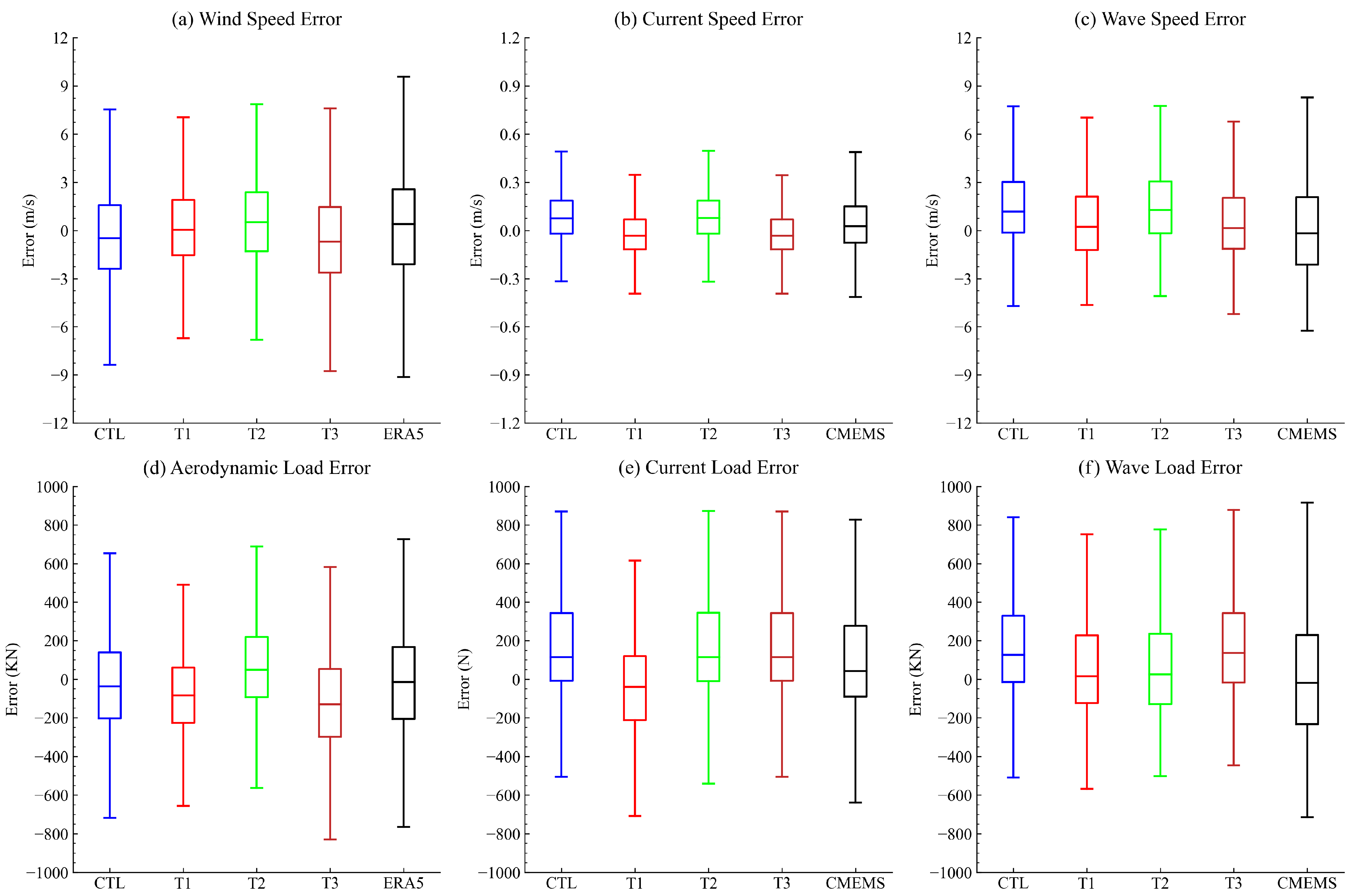
4.1. Error Distribution of Forecasted Dynamic Factors

Based on observational data from the Cangnan wind farm, the total number of samples for wind speed, wave speed, and current speed was 1403, 1357, and 1357, respectively. The quality control module identified 15, 32, and 21 samples as anomalous ones for each variable, respectively, while the total number of missing samples for linear interpolation filling was 38, 84, and 84. Among the valid observations, the mean wind, wave, and current speed were 8.5 m/s, 5.38 m/s, and 0.28 m/s, respectively, with corresponding maximum values of 22.87 m/s, 13.17 m/s, and 0.77 m/s.

Figure 3 presents vertical profiles of wind speed and current speed at 00:00, 06:00, 12:00, and 18:00 UTC on 6 April 2023. Figure 3a shows wind speed profiles at all observed heights, while Figure 3b displays current speed profiles at all observed depths. It can be seen that wind speed generally increases with height, with the 06:00 UTC time corresponding to 14:00 local time, when atmospheric stratification is unstable, causing a decrease in wind speed above 150 m. The current speed profile decreases gradually with increasing depth, and diurnal variations are not significant.

Figure 4 presents box plots illustrating the 24 h forecast errors for the speeds and corresponding dynamic loads of wind, current, and wave components. In each box plot, the upper and lower whiskers represent the maximum and minimum forecast errors, respectively; the central line within the box denotes the median error, while the upper and lower edges correspond to the upper and lower quartiles of the error distribution. To compute the forecast errors, observational data included wind speed measurements at 19 different heights, current speed at 7 depths, and wave speed at the sea surface during the validation period. For consistency and comparability, the model forecast outputs were interpolated to match the corresponding observational heights and depths. Additionally, the forecast errors of ERA5 reanalysis data relative to observations were included as a reference baseline.

Figure 4a shows the distribution of wind speed forecast errors at all observation heights. The wind speed error distribution range for all tests was roughly between −8.0 m/s and 8.0 m/s, with medians close to zero. Among them, the error distributions for the CTL, T1, T2, and T3 tests were relatively concentrated. Compared to the CTL test, the T1 test, which considers both data assimilation and error correction, showed a significantly reduced error range, a shorter box length, and a median closer to zero, indicating a reduction in overall bias. The T2 test, which only considered the assimilation process, showed a smaller error range compared to the CTL test, but the overall improvement was not significant. For the T3 test, which considered only the error correction process without assimilation, the overall error distribution was similar to that of the T1 test, but the improvement was not as pronounced, indicating that the error correction process had a more significant impact on forecast accuracy than the assimilation process. Additionally, the error range for the ERA5 data was significantly wider compared to the three simulation tests, indicating greater overall error fluctuation.

Figure 4b shows the distribution of current speed forecast errors at all observation depths, with the error for CMEMS data included as a reference; Figure 4c presents the distribution of wave speed forecast errors, also including CMEMS data. The error distributions for current speed and wave speed were similar to those for wind speed (Figure 4a), with the T1 test showing the most concentrated errors and the smallest fluctuations. The current speed error distribution (Figure 4b) indicated that the T2 test’s error levels were nearly identical to those of the CTL test, suggesting that atmospheric data assimilation had a much smaller impact on current speed than on wind speed and wave speed. In the case of minimal atmospheric assimilation influence, the error distribution for the T3 test became very similar to that of the T1 test.

Figure 4d–f shows the box plots of aerodynamic load, current load, and wave load forecast errors at the location of the Cangnan Offshore Wind Farm. Aerodynamic loads include both blade load and tower load. In Figure 4d, the aerodynamic load forecast error distributions for the CTL, T1, T2, and T3 tests were similar to those in Figure 4a, with the T1 test still outperforming the others. The T3 test showed more negative bias, resulting in an average error level lower than that of the CTL test, which was probably related to the segmented calculation of rotor thrust coefficient. The current load errors in Figure 4e and the wave load errors in Figure 4f were consistent with the errors in Figure 4b,c, indicating that the statistical distributions of the corresponding load errors remain unchanged.

4.2. Statistical Characteristics of Predicted Dynamic Factors

Figure 5 shows the profile of the RMSEs for the 24 h forecast during the validation period within 230 m above the surface. The formula for calculating the RMSE is as follows:

$$RMSE=\sqrt{{\displaystyle \frac{{\displaystyle \sum _{i=1}^n{\left(X_{obs,i}-X_{model,i}\right)}^2}}{n}}}$$

(7)

Here, i represents any moment within the validation period, and $\mathrm{n}$ is the total duration of the validation period.

For comparison convenience,

Table 2. The average RMSEs of wind, wave, current speed, and their corresponding loads for the forecasting tests.

	CTL	T1	T2	T3	ERA5	CMEMS
Wind speed	3.51 m/s	2.68 m/s	2.97 m/s	3.19 m/s	3.55 m/s	-
Aerodynamic load	319.21 kN	275.59 kN	278.38 kN	344.82 kN	319.93 kN	-
Wave speed	3.19 m/s	2.83 m/s	3.28 m/s	2.77 m/s	-	3.23 m/s
Wave load	373.58 kN	335.85 kN	382.93 kN	327.67 kN	-	377.48 kN
Current Speed	0.17 m/s	0.13 m/s	0.16 m/s	0.14 m/s	-	0.17m/s
Current load	336.26 N	315.51 N	336.76 N	312.78 N	-	334.02 N

also lists these average RMSE values.

In Figure 5a, the wind speed error profile is displayed. The CTL, T1, T2, T3, and ERA5 data are represented by blue, red, green, brown, and black, respectively. Above 50 m, the RMSE values for all four forecast tests (CTL, T1, T2, T3) and ERA5 data showed very little variation and similar trends with height. As height increased, the error of ERA5 data became noticeably larger than the forecasts of the four tests. Compared to the blue CTL test, the wind speed RMSE values of the T1, T2, and T3 tests were lower. The average RMSE of the T1 test within the 230 m height was 2.68 m/s, which was a reduction of approximately 24% and 25% compared to the CTL test (3.51 m/s) and ERA5 data (3.55 m/s), respectively. The data assimilation in the T2 test had a positive impact, and the error (averaging 2.97 m/s) was lower than the CTL test at all heights. For the T3 test, the average RMSE was 3.19 m/s, with its profile shape similar to that of the T1 test. Below 50 m, the small difference between the T3 and T1 tests indicated that the error correction process played a greater role near the sea surface.

Figure 5b shows the RMSE profile for current speed, with the error for CMEMS data included as a reference. The errors for all tests were observed to decrease in depth. The RMSEs for the CTL (blue line) and T2 test (green line) were nearly identical, with average values of 0.17 m/s and 0.16 m/s, respectively. The RMSE for the T1 (red line) and T3 tests (brown line) were slightly lower, with values of 0.13 m/s and 0.14 m/s. The assimilation of wind speed data seemed to have a minimal effect on current speed simulations.

Figure 5c shows the RMSE profile for aerodynamic loads. Since blade loads only exist within the height range swept by the blades, the aerodynamic load below 150 m is mainly due to tower load. The error profile showed a clear discontinuity near 150 m height. For ease of comparison, the error profile below 150 m was enlarged and shown separately. Below 150 m, the error for the T1 test (red line) was lower than for other tests and ERA5 data, consistent with the results in Figure 4a. However, the average RMSEs for the T3 test and ERA5 data below 150 m were 0.096 kN and 0.11 kN, respectively, significantly lower than the values for the T2 and CTL test (0.16 kN and 0.19 kN). Above 150 m, the T3 test showed an increase in error, likely due to the segmented load calculation, with an average RMSE of 344.82 kN. For the other tests, as height increased, the error profile for the T2 test gradually approached that of the T1 test, with average RMSE values of 278.38 kN and 275.59 kN, respectively, indicating that the assimilation process played a more significant role in load calculation at these heights. On average, the RMSEs for the T1, T2, and T3 tests were reduced by about 13%, 12%, and −8% compared to the CTL test.

Figure 5d shows the RMSE profile for current loads. Between 16 m depth and 4 m depth, the RMSEs for T1 and T3 were slightly higher than for the others, but on average, the RMSEs for T1 and T3 were 313.51 N and 312.78 N, respectively, slightly lower than for the others (CTL: 336.26 N, T2: 336.76 N, CMEMS: 334.02 N). The RMSEs for the T1, T2, and T3 tests were reduced by approximately 6.7%, −0.1%, and 6.9% compared to the CTL test.

For wave speed forecasts, the RMSEs for the various tests were as follows: 3.19 m/s (CTL), 2.83 m/s (T1), 3.28 m/s (T2), 2.77 m/s (T3), and 3.23 m/s (CMEMS). Similarly, the RMSEs for wave load forecasts were 373.58 kN (CTL), 335.85 kN (T1), 382.93 kN (T2), 327.67 kN (T3), and 377.48 kN (CMEMS). The results for wave speed and wave load forecasts were generally consistent, with the T1 test showing lower errors than the CTL test and CMEMS data. However, the assimilation of atmospheric data slightly increased the wave simulation errors, and the T3 test, relying solely on error correction, showed even lower errors. The RMSEs for the T1, T2, and T3 tests were reduced by about 10.09%, −2.50%, and 12.29%, respectively, compared to the CTL test.

In addition to RMSE, Figure 6 presents the temporal correlation coefficient (CC) profiles between the forecast results and the observations during the validation period. For comparison convenience,

Table 3. The average CCs of wind, wave, current speed, and their corresponding loads for the forecasting tests.

	CTL	T1	T2	T3	ERA5	CMEMS
Wind speed	0.47	0.65	0.63	0.44	0.47	-
Aerodynamic load	0.38	0.53	0.51	0.39	0.42	-
Wave speed	0.16	0.11	0.14	0.12	-	0.08
Wave load	0.18	0.11	0.11	0.17	-	0.12
Current Speed	0.28	0.18	0.27	0.19	-	0.19
Current load	0.24	0.17	0.24	0.18	-	0.21

also presents the average CC values. The formula for calculating the correlation coefficient is as follows:

$$CC={\displaystyle \frac{{\displaystyle {\sum }_{i=1}^n(x_{mi}-\overline{x_m})(x_{oi}-\overline{x_o})}}{\sqrt{{{\displaystyle {\sum }_{i=1}^n\left(x_{mi}-\overline{x_m}\right)}}^2\cdot {\displaystyle {\sum }_{i=1}^n{\left(x_{oi}-\overline{x_o}\right)}^2}}}}$$

(8)

Figure 6a shows the vertical profile of the average wind speed correlation coefficient. The forecasted wind speed for all tests had a high correlation with the observations. The assimilation process appeared to help make the forecast results’ temporal variability closer to the observations. The T1 and T2 tests showed the highest correlation with the observations, with average values of 0.65 and 0.63, respectively. The T3 test, which only considered error correction, reduced the forecast error but did not significantly improve the correlation coefficient. The correlation coefficients for all tests showed little variation with height, and the ERA5 data shows similar values to the CTL test.

Figure 6b shows the vertical profile of the current speed forecast correlation coefficient. Due to the weak impact of atmospheric assimilation on current speed simulation, the correlation coefficients for the T2 and CTL tests were nearly identical, with average values of 0.27 and 0.28, respectively. The correlation coefficients for the T1 and T3 tests decreased compared to the CTL test, with values of 0.18 and 0.19, respectively. This result was consistent with the findings in Figure 6a, indicating that the GRU error correction module was more inclined to correct the mean and error of the forecast results, but did not significantly improve the variance and temporal variability of the forecasts.

Figure 6c shows the vertical profile of the aerodynamic load forecast correlation coefficient. Below 150 m, where only tower loads were considered, the correlation coefficient for the T1 test was better than the other tests. Above 150 m, the T3 test had the lowest correlation coefficient, while the T1 and T2 tests showed relatively higher correlation coefficients.

The vertical profile of the current load forecast correlation coefficient (Figure 6d) was roughly consistent with the results in Figure 6b, with all correlation coefficient values being below 0.4. The correlation coefficients for the CTL and T2 tests were slightly higher, both at 0.24, while the T1 and T3 tests had weaker correlations with the observations, with values of 0.17 and 0.18, respectively. The CMEMS data had a correlation coefficient of 0.21, which was generally lower than the CTL and T2 tests.

Additionally, the wave speed forecast correlation coefficients for all tests were as follows: 0.16 (CTL), 0.11 (T1), 0.14 (T2), 0.12 (T3), and 0.08 (CMEMS). The wave load forecast correlation coefficients were generally consistent, with values of 0.18 (CTL), 0.11 (T1), 0.11 (T2), 0.17 (T3), and 0.12 (CMEMS). The correlation coefficients for all tests were relatively low, which was also due to the high randomness of the wave processes and the difficulty in simulating them. Compared to the other test, although the T1 test showed a reduction in RMSE, the correlation coefficient did not improve and was even slightly lower than the CTL test.

Figure 7 shows the Taylor diagrams for the 24 h forecasts of wind speed, current speed, wave speed, and their corresponding loads. The Taylor diagram contains two dimensions: one dimension is the standard deviation, and the other dimension is the correlation coefficient. Figure 7a presents the Taylor diagram for forecasted wind speed at 230 m height. The accuracy of the CTL test and ERA5 data was nearly identical, with the standard deviation showing minimal difference from the observation. The assimilation process improved the correlation coefficient while maintaining the standard deviation of the data relatively unchanged, making the T2 test closer to the reference point compared to other tests. The error correction process seemed to reduce the deviation of the forecast results, with the standard deviations of the T1 and T3 tests being lower than those of the others.

Figure 7b presents the Taylor diagram for forecasted current speed. The correlation coefficients for all four forecast results were relatively low, and the standard deviations were also lower than the observations, indicating that the forecast current speed had relatively weak temporal variability. Due to the limited impact of atmospheric assimilation on current speed forecasts, the T2 and CTL results were nearly identical. The T1 and T3 tests, however, show lower values for both the correlation coefficient and standard deviation, and were farther from the reference point. The forecast wave speed in Figure 6c was consistent with the results in Figure 7b, with the only difference being a lower correlation coefficient. Notably, in Figure 7a–c, the standard deviations of both the T1 and T3 tests were lower than those of the T2 or CTL tests before correction, suggesting that during the correction process, the fluctuation amplitude of the forecast wind speed over time was somewhat diminished.

Figure 7d–f shows the Taylor diagrams for aerodynamic, current, and wave loads, respectively. The forecast aerodynamic load for the T1 test was closer to the reference point when compared to the others. However, for the current load and wave load distributions, the T1 tests did not show a significant advantage over the others, indicating that the integration of error correction with atmospheric assimilation did not improve the correlation coefficients and standard deviations of the current speed and wave speed forecasts.

$$\mathrm{The}\mathrm{variance}(\mathrm{VAR})\mathrm{can}\mathrm{be}\mathrm{calculated}\mathrm{by}:\mathrm{VAR}={\displaystyle \frac{1}{n}}{\displaystyle {\sum }_{i=1}^n{\left(x_i-\overline{x}\right)}^2}$$

(9)

To clearly illustrate the variance characteristics of each test and the reanalysis datasets,

Table 4. The variances of wind, wave, current speed, and their corresponding loads for the forecasting tests.

	OBS	CTL	T1	T2	T3	ERA5	CMEMS
Wind speed (m2/s2)	3.21	3.43	2.34	3.49	2.04	3.42	-
Aerodynamic load (106N2)	284.69	270.74	277.69	294.96	236.27	289.94	-
Wave speed (m2/s2)	2.56	1.09	0.98	1.13	0.95	-	1.88
Wave load (106N2)	299.78	110.96	102.29	111.59	101.59	-	201.27
Current Speed (m2/s2)	0.13	0.093	0.092	0.094	0.091	-	0.12
Current load (N2)	298.31	140.24	228.32	140.59	227.83	-	244.22

presents the variances of wind speed, wave speed, current speed, and their corresponding loads. The variance calculation formula is provided in Equation (9). As shown in Table 4, the wind speed forecast variances from the control test (CTL), the assimilation test (T2), and ERA5 were generally consistent with observations. In contrast, the variances in T1 and T3, after deep learning-based error correction, were significantly reduced. For current speed and wave speed, the variances in CMEMS data were clearly closer to observations compared to those in the forecast tests. After load calculations, the variances for all datasets were amplified to varying degrees. Among them, the aerodynamic load variance from ERA5 and the wave load variance from CMEMS remained the closest to observations. However, the current load variance from CMEMS deviated further from the observed values. Overall, in terms of data variability, the ERA5 and CMEMS reanalysis datasets outperformed the COAWST model’s forecasts.

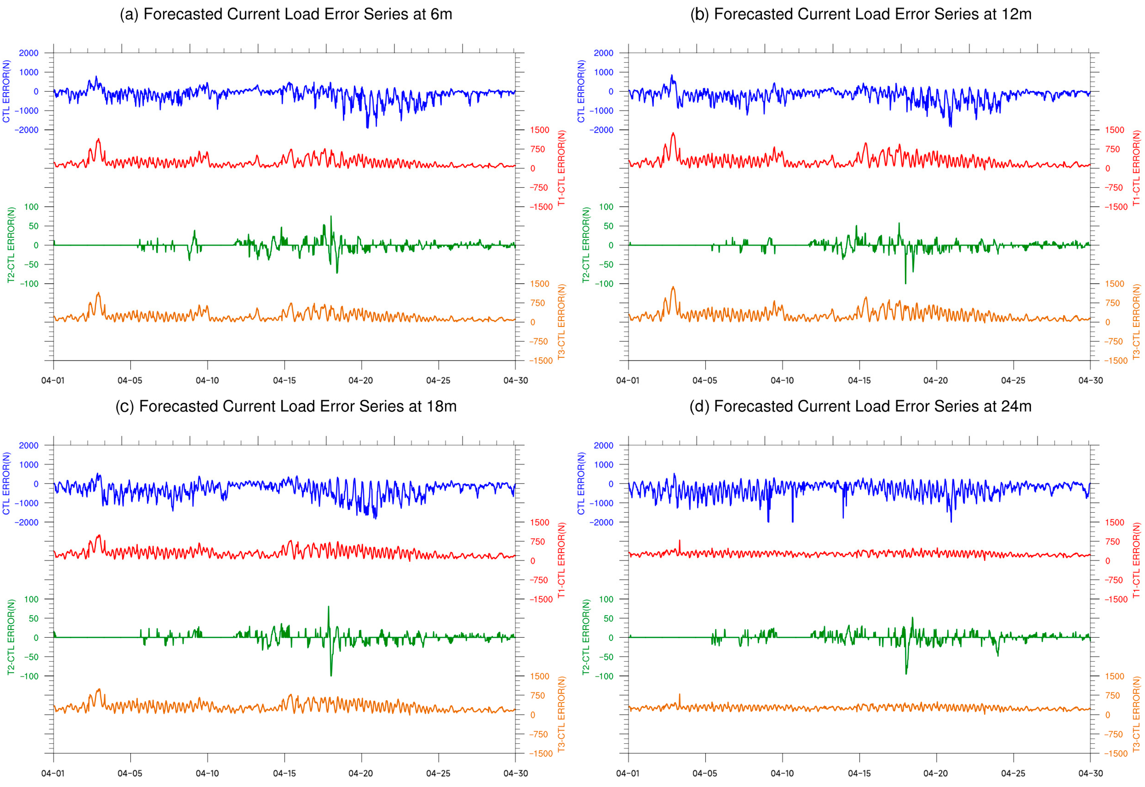
4.3. Temporal Variability of Predicted Dynamic Factors

In addition to the aforementioned statistical indicators, the time series of dynamic load variations during the validation period is also presented. Figure 8 shows the 24 h forecast error time series for aerodynamic load at heights of 60 m, 120 m, 180 m, and 230 m. In Figure 8a, the error time series between CTL and the observations (CTL–OBS) at 60 m is shown, along with the differences between T1, T2, and T3 tests and the CTL one (T1–CTL, T2–CTL, T3–CTL). By comparing the error of the CTL test with the relative changes in the other three tests, the improvements compared to the original model can be assessed. The average value of the CTL–OBS error series during the validation period was 1157.69 N. In most cases, the forecast error of the CTL test showed minimal variation. Around 5 April and 19 April, the wind speed in the study domain significantly increased, with the average wind speed reaching 13.41 m/s and 12.83 m/s, respectively, resulting in large fluctuations in the error.

The average differences (T1–CTL, T2–CTL, T3–CTL) during the validation period were −1074.32 N, −333.96 N, and −889.26 N, respectively, all of which reduced the error of the CTL test. The difference series for all three tests showed a high negative correlation with the CTL error series, with values of −0.81, −0.43, and −0.79, respectively. This negative correlation indicated that when the CTL error changed, the errors in the other three tests generally reduced the amplitude of the CTL error changes. The negative correlation between the T1–CTL and T3–CTL series with the CTL–OBS series was notably stronger, suggesting that the error correction process in the T1 and T3 tests effectively reduced the mean error while also dampening the fluctuations of the original forecast results. The fluctuation amplitude of the T2–CTL series, which did not include error correction, was clearly higher than that of the T1–CTL and T3–CTL series. It indicated that the assimilation process did not alter the fluctuation characteristics of the forecast, but its phase changes did not fully match the CTL–OBS series, resulting in a less noticeable reduction in error.

Figure 8b shows the time series for CTL–OBS, T1–CTL, T2–CTL, and T3–CTL at 120 m height. The series were roughly the same as in Figure 8a, with no significant change. Their average values were 1411.52 N, −1039.98 N, −407.188 N, and −1084.24 N, respectively. The correlation coefficients between T1–CTL, T2–CTL, T3–CTL, and CTL–OBS were −0.81, −0.43, and −0.81, respectively.

After incorporating blade load calculations, the overall aerodynamic load forecast error no longer showed a simple positive correlation with wind speed errors. As shown in Figure 8c, the average error for the CTL test in aerodynamic load forecasting at 180 m height was 336.58 kN. The differences between the T1, T2, and T3 tests and the CTL one were 438.60 kN, −915.69 kN, and 1292.69 kN, respectively. Their fluctuation of series was significantly higher compared to Figure 8a,b. The correlation coefficients between the T1–CTL, T2–CTL, and T3–CTL series and CTL–OBS dropped to −0.59, −0.56, and −0.29, respectively. The fluctuation of the T2–CTL and T1–CTL series was significantly higher than that of the T3–CTL series, suggesting that the T1 test was able to effectively enhance the temporal variability of the data, which was consistent with the standard deviation results in Figure 7d. The time series at 230 m height (Figure 8d) was similar to that in Figure 8c. The average values for the four series were 248.88 kN (CTL–OBS), 577.05 kN (T1–CTL), −877.31 kN (T2–CTL), and 1412.92 kN (T3–CTL). The correlation coefficients between CTL–OBS and the latter three series were −0.59, −0.58, and −0.34, respectively.

Similarly to Figure 8, Figure 9 shows the time series of current load forecast errors for the CTL test, along with the difference series between T1, T2, T3, and CTL at depths of 6 m, 12 m, 18 m, and 24 m during the validation period. In Figure 9a, the average values of the four series were −155.51 N (CTL–OBS), 216.42 N (T1–CTL), −0.51 N (T2–CTL), and 217.46 N (T3–CTL). The T1 and T3 tests effectively improved the negative error of the CTL test, but their temporal variability did not align with the CTL error. The correlation coefficients between T1–CTL, T2–CTL, T3–CTL, and CTL–OBS were 0.32, 0.056, and 0.32, respectively. The T2–CTL series consistently fluctuated around zero, with almost no correlation with the CTL error series, indicating that atmospheric assimilation had little impact on the current speed simulation. At certain moments, the T2–CTL series showed stronger fluctuations, but it remained centered around zero, suggesting that it was more influenced by short-term environmental changes rather than changes to the CTL error. Figure 9b–d shows similar results to Figure 9a. As depth increased, the fluctuation of the time series for each group gradually decreased. For the average error values, the CTL test showed a negative current load error at all depths. After correction by the T1 and T3 tests, this negative error was effectively eliminated, but the correlations between the CTL–OBS and the T1–CTL, T2–CTL, and T3–CTL series were still low, ranging from 0.2 to 0.3.

Figure 10 presents the time series of wave load for the four tests, with average values of −197 kN (CTL–OBS), 106.7 kN (T1–CTL), −1.09 kN (T2–CTL), and 108.21 kN (T3–CTL). The error correction module’s strategy for wave load error correction was very conservative, only correcting the mean error of the CTL test, contributing little to the reduction in temporal variability. The difference series for the T3 test, which only considered error correction, showed lower temporal variability compared to the CTL test, resulting in the T1–CTL and T2–CTL series showing extremely similar variability, aside from the mean differences. In other words, the T1–CTL series suggested that the data assimilation process and error correction process together were able to present a combined effect in wave load forecasting.

5. Discussion and Conclusions

This study developed a prediction model for turbine environmental dynamic loads in offshore wind farms based on the COAWST ocean-atmosphere coupled model, a GRU algorithm, and a three-dimensional ensemble variational atmospheric data assimilation system. Four sensitivity tests were designed for the Cangnan offshore wind farm region: (1) the CTL test utilizing the original COAWST forecast, (2) the T1 test incorporating both atmospheric assimilation and GRU-based error correction, (3) the T2 test applying only atmospheric assimilation, and (4) the T3 test employing only error correction. Comparative analysis of these tests enabled a systematic evaluation of the contributions of each component to forecast improvement.

Compared with previous studies, this study revealed through a series of tests that wind assimilation improved the prediction of aerodynamic loads on wind turbines. This improvement was able to be further enhanced when combined with bias correction, leading to higher forecasting accuracy. However, wind assimilation had a limited impact on wave and current loads on offshore wind turbines. Although wind assimilation did not significantly reduce errors in wave load prediction, it helped mitigate the drawback of reduced temporal variability caused by deep learning-based bias correction. In terms of engineering application, this study proposed a novel approach that integrated data assimilation and deep learning, which had the potential to significantly reduce forecast errors and improve the accuracy of turbine dynamic load prediction.

However, the experimental results presented in this study still contained certain uncertainties, primarily related to data, model configurations, and experimental design.

In terms of data, acquiring dense vertical observations for a specific region is challenging. As a result, this study conducted validation using data from a single observation site, and the applicability of the forecast results to other regions remains to be verified. For the observations at the Cangnan wind farm, although the 19-layer wind measurements and seven-layer current observations provided sufficient vertical resolution, the height and depth levels were rather uniformly distributed. This configuration may not adequately capture turbulent processes in the atmospheric boundary layer or the current shear effects in the subsurface ocean layer.

Additionally, the presence of the wind turbine tower introduced some risks in wind observation, which probably led to an underestimation of wind speed observation from certain directions. Figure 11 shows the statistical distribution of observed wind direction during the validation period in the Cangnan wind farm. Located in a monsoon region, the prevailing winds were concentrated in the 0~60° and 180~240° sectors. Observations within the 120~150° range were notably sparse, which may be influenced not only by prevailing wind patterns but also by structural interference from the turbine itself.

As a result, the actual mean wind speed was probably higher than what was recorded by the sensors. In this study, all forecast tests tended to exhibit positive biases in wind speed compared to the observations. Therefore, the true forecast performance may be even better than what was reported.

Other risks for observation data are associated with the sensors themselves, especially for the underwater sensors. The harsh underwater environment posed significant challenges to the long-term stable operation of buoys and subsurface buoys. A large proportion of missing data introduced uncertainties into the validation process of this study. Due to objective constraints, the observational data used in this study cover only one year, and some months suffer from substantial data gaps caused by equipment failures. Consequently, the month with the most complete observations was selected for model validation. However, the short validation period introduces uncertainty to the conclusions. The absence of data from different seasons and the lack of extreme weather events, such as typhoons, during the validation period further reduce the representativeness and robustness of the study’s findings. In future work, we plan to collect longer-term observations for more comprehensive validation and systematic model evaluation. In addition, the vertical distribution of observation heights and depths at the Cangnan Wind Farm is relatively uniform, which may overlook key physical processes at certain critical levels and reduce simulation accuracy.

From a modeling perspective, the COAWST system has difficulty capturing small-scale physical processes in atmospheric variables, which may result in the omission of important factors during the calculation of dynamic loads. In future work, we plan to further optimize and improve the COAWST model to enhance its capability in resolving finer-scale processes. To improve the accuracy of wave and current forecasts, we also intend to incorporate additional wave and ocean data assimilation systems, integrating satellite observations and other datasets to refine the prediction outputs. Moreover, the accuracy of deep learning models is partially dependent on the training strategy employed. Previous studies have shown that feature extraction and classification techniques, such as data clustering and principal component analysis (PCA), can significantly improve model performance. These methods were not implemented in the current study, and future work will address this limitation with dedicated investigations. In the early phase of this research, we evaluated the correction performance of several algorithms, including BP (Backpropagation), Random Forests, LSTM, and CNN. Among these, the GRU-based approach demonstrated the lowest prediction error and was ultimately selected for the final correction procedure. However, we observed that all neural network-based correction methods tend to suppress the temporal variability of the corrected forecasts, which poses challenges in predicting extreme events. To mitigate the limitations of a single learning model under varying meteorological conditions, future improvements will explore the use of ensemble learning strategies, modifications to neural network architectures, and hybrid approaches. These enhancements are expected to improve model robustness and better capture the dynamic characteristics of atmospheric and oceanic processes.

In terms of experimental design, this study conducted horizontal comparisons using reanalysis data but did not quantitatively assess how errors in reanalysis data propagate into the dynamic load calculations. Future work will address this issue by systematically evaluating the impact of reanalysis uncertainties on load prediction accuracy.

To further verify the model’s performance at other sites, we collected observational data from a buoy station (Nanji) located within the study area. The buoy data, obtained from the National Marine Data Center of China (https://mds.nmdis.org.cn, accessed on 19 June 2025), were used to validate 10 m wind speed and wave phase speed. The station’s location is shown in Figure 2. During the validation period, the mean absolute errors (MAEs) of 10 m wind speed at the buoy site were 2.01 m/s (CTL), 1.75 m/s (T1), 1.87 m/s (T2), and 1.85 m/s (T3), while the MAEs for wave phase speed were 1.82 m/s (CTL), 1.77 m/s (T1), 1.88 m/s (T2), and 1.79 m/s (T3). These results are generally consistent with those at the Cangnan offshore wind farm. The T1 test exhibited the lowest prediction errors for both wind and wave speed across both sites. The T3 test, which applied only error correction, also achieved notable improvements, though slightly less than T1. In contrast, the T2 test, which applied only wind assimilation, showed a comparable improvement in 10 m wind speed but yielded limited enhancement in wave speed predictions, with errors slightly higher than those in the CTL run. For the four forecast tests, the correlation coefficients of the 10 m wind speed were 0.32 (CTL), 0.37 (T1), 0.32 (T2), and 0.36 (T3), respectively. The wave speed correlation coefficients were 0.12 (CTL), 0.09 (T1), 0.10 (T2), and 0.10 (T3). These correlation coefficients showed a pattern similar to that of the mean absolute errors, with wind speed correlations generally higher than those of wave speed. These findings suggest that the proposed forecasting framework can reduce the original prediction errors at multiple sites. However, the magnitude and consistency of the improvements vary among different locations, indicating that the model’s performance still carries significant spatial uncertainty. Future studies will conduct additional simulations and validations across broader regions to enhance the reliability and generalizability of the results.

In addition, the noise check for the T1 test was performed. The forecast time series of aerodynamic load at 180 m height, current load at 18 m depth, and wave load were selected for autocorrelation analysis at first. Figure 12a–c shows the distributions of the autocorrelation functions (ACF) for the three types of loads. Most of the autocorrelation values fell outside the 95% confidence intervals, indicating that the forecast results were non-stationary time series. Subsequently, the three time series were differenced to address non-stationarity: the aerodynamic load and wave load forecasts were processed using first-order differencing, while the current load forecast was processed using seasonal differencing. The ACF distributions after processing are shown in Figure 12d–f. After differencing, most autocorrelation coefficients fall within the 95% confidence bounds (i.e., within ±2 standard deviations), suggesting that the differenced series can be considered stationary. Furthermore, the Box–Pierce test was performed with lag orders of three and six. In both cases, the p-values were less than 0.05, indicating that the null hypothesis of white noise was rejected at the 95% confidence level. This confirmed that the three forecast time series were not purely random (white noise) processes. The results for the CTL, T2, and T3 tests were consistent with those of T1, suggesting that the forecasts contained meaningful temporal structure rather than being random noise.

The conclusions of this study are as follows:

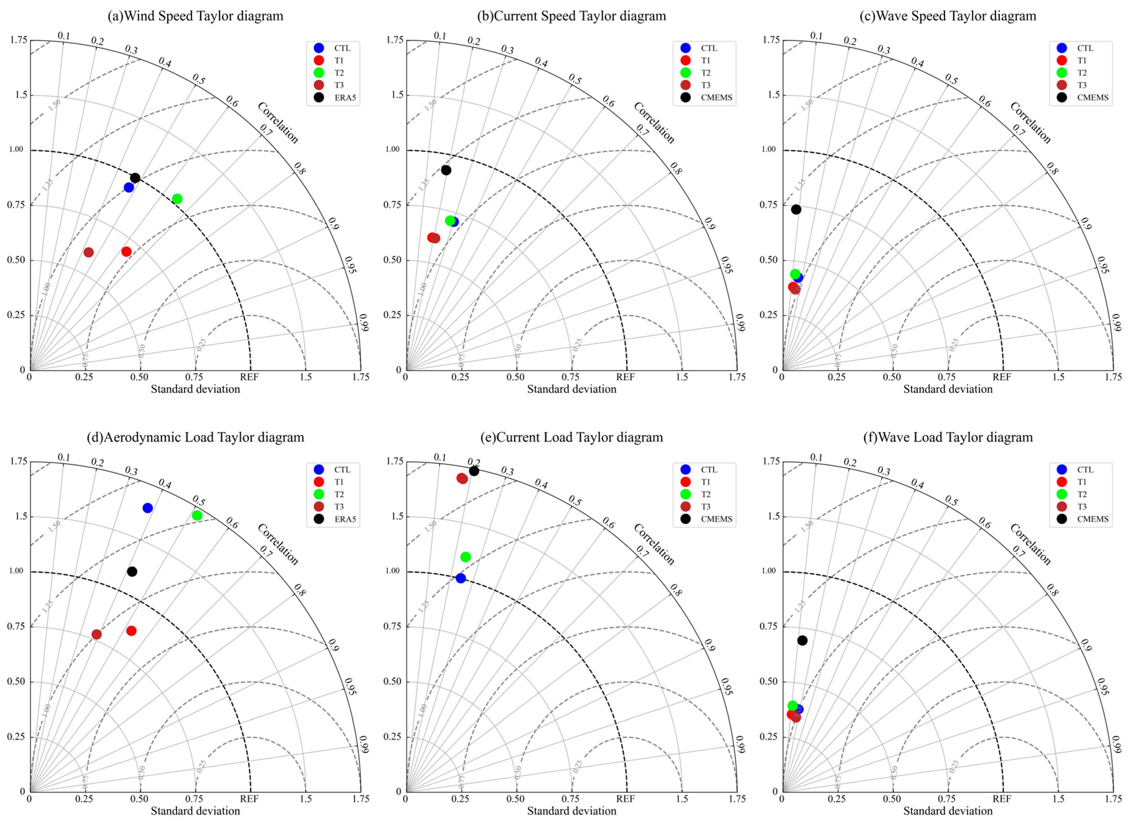
• The atmospheric assimilation process effectively reduces forecasting errors, particularly for aerodynamic loads on offshore wind turbines, and can be further enhanced through integration with deep learning-based error correction. During validation, the T3 test, which applied only error correction, reduced RMSEs of aerodynamic, current, and wave loads by approximately 8%, 6.9%, and 12.9%, respectively, compared to the control test (CTL). In contrast, the T1 test, which incorporated both atmospheric assimilation and error correction, achieved greater reductions of about 13%, 6.7%, and 10.09%, respectively. Overall, the combined approach produced forecasts that were more consistent with observational data and outperformed ERA5 and CMEMS reanalysis datasets across multiple evaluation metrics, including RMSE and correlation coefficient.
• While atmospheric assimilation effectively reduced forecast errors for environmental wind speed and aerodynamic loads at turbine height, it had a limited impact on the forecast accuracy of current speed, wave speed, and their associated dynamic loads. In the case of wave loads, atmospheric assimilation introduced minor fluctuations in the simulation results, but the overall changes in error and standard deviation were not substantial. For current load forecasts, the differences caused by atmospheric assimilation were negligible and could even be considered as noise-level effects.
• The error correction module based on the GRU algorithm, although effective in reducing dynamic load forecasting errors, primarily corrects the mean bias of the forecast results. This process tends to suppress the temporal variability or fluctuations in the forecasts. Consequently, the corrected results exhibit limited improvement in terms of correlation coefficient and standard deviation. In contrast, atmospheric assimilation does not significantly alter the temporal variability of the original forecast. In the case of aerodynamic load forecasting, where the improvement was most significant, the integration of atmospheric assimilation effectively compensated for the decline in the correlation coefficient between the corrected forecasts and actual observations. However, for wave and current load forecasts, atmospheric assimilation had minimal impact on enhancing the correlation coefficient.
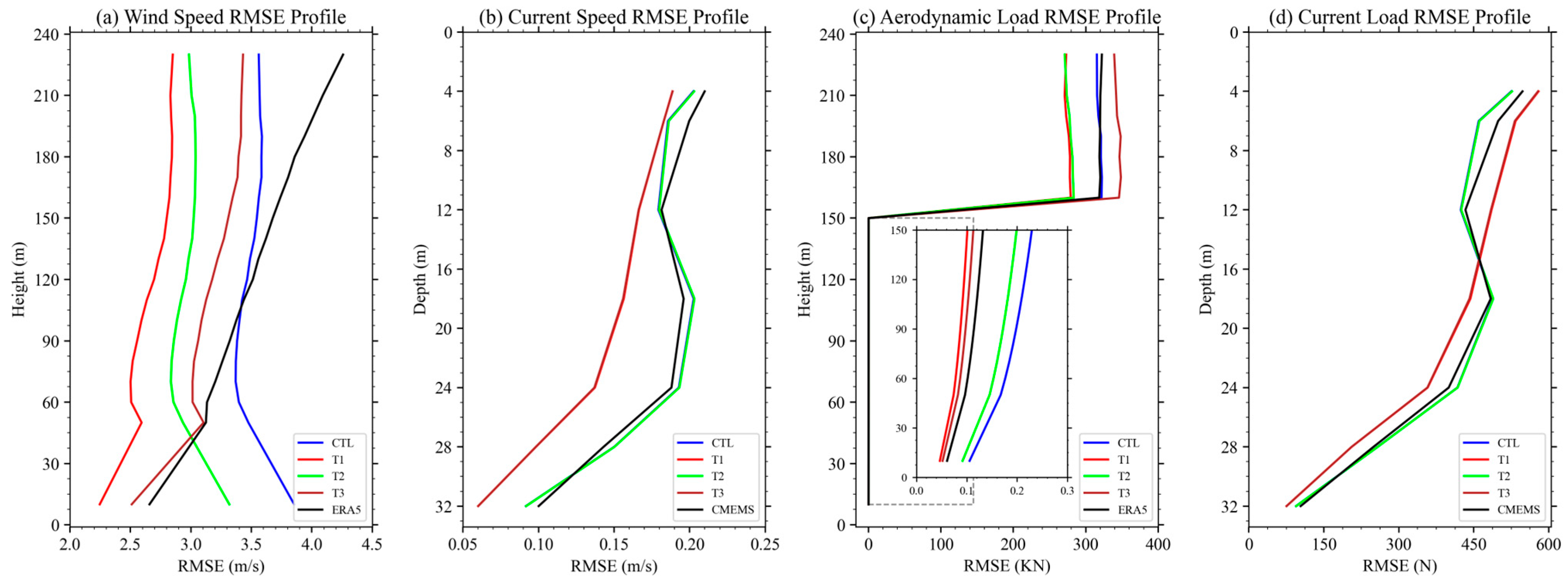
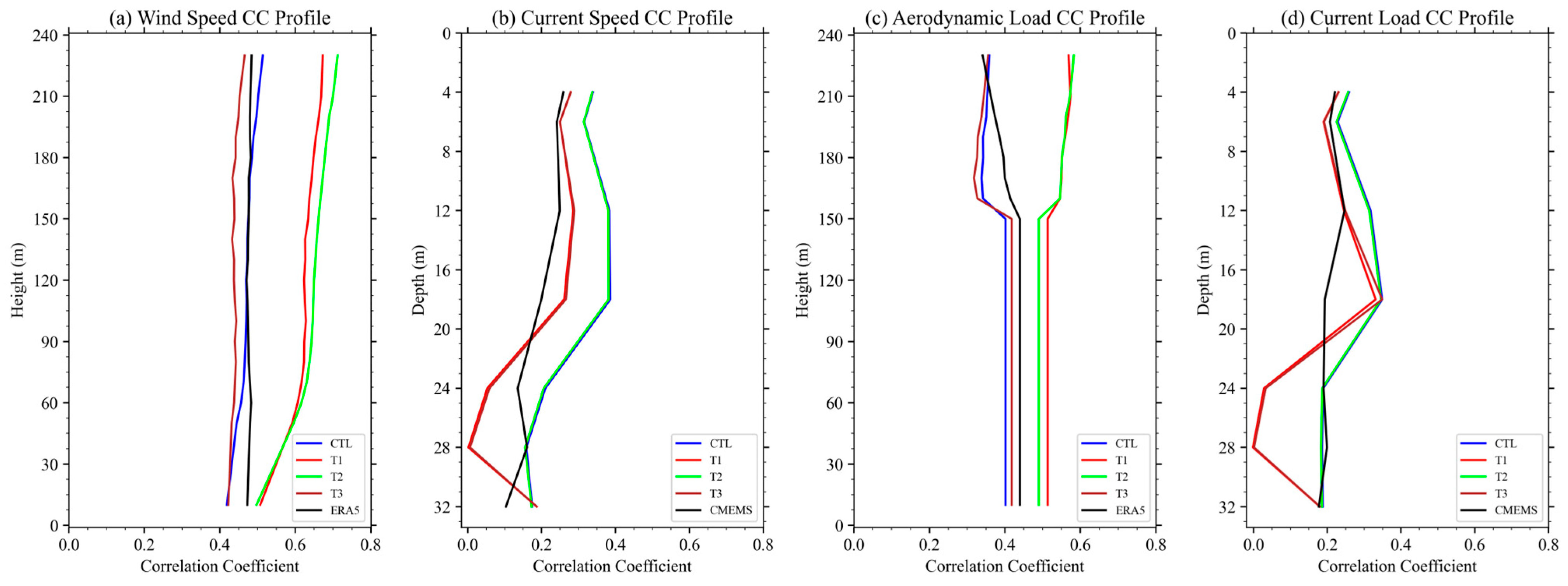
• The forecast errors for aerodynamic and current loads exhibited vertical variations that were generally consistent with the magnitude of their baseline values. At higher altitudes or shallower depths—where wind and current speeds tend to be greater—the corresponding load forecast errors were also relatively larger. However, the vertical variation in correlation coefficients was minimal, indicating that the forecast accuracy, in terms of trend consistency with observations, remained relatively stable across different heights.

References

1. Liu, H.; Mi, X.; Li, Y. Smart Deep Learning Based Wind Speed Prediction Model Using Wavelet Packet Decomposition, Convolutional Neural Network and Convolutional Long Short Term Memory Network. Energy Convers. Manag. 2018, 166, 120–131. [Google Scholar] [CrossRef]
2. Bilgili, M.; Yasar, A.; Simsek, E. Offshore Wind Power Development in Europe and Its Comparison with Onshore Counterpart. Renew. Sustain. Energy Rev. 2011, 15, 905–915. [Google Scholar] [CrossRef]
3. Jahani, K.; Langlois, R.G.; Afagh, F.F. Structural Dynamics of Offshore Wind Turbines: A Review. Ocean. Eng. 2022, 251, 111136. [Google Scholar] [CrossRef]
4. Marino, E.; Giusti, A.; Manuel, L. Offshore Wind Turbine Fatigue Loads: The Influence of Alternative Wave Modeling for Different Turbulent and Mean Winds. Renew. Energy 2017, 102, 157–169. [Google Scholar] [CrossRef]
5. Moulas, D.; Shafiee, M.; Mehmanparast, A. Damage Analysis of Ship Collisions with Offshore Wind Turbine Foundations. Ocean. Eng. 2017, 143, 149–162. [Google Scholar] [CrossRef]
6. Lian, J.; Jia, Y.; Wang, H.; Liu, F. Numerical Study of the Aerodynamic Loads on Offshore Wind Turbines under Typhoon with Full Wind Direction. Energies 2016, 9, 613. [Google Scholar] [CrossRef]
7. Chen, X.; Li, C.; Xu, J. Failure Investigation on a Coastal Wind Farm Damaged by Super Typhoon: A Forensic Engineering Study. J. Wind. Eng. Ind. Aerodyn. 2015, 147, 132–142. [Google Scholar] [CrossRef]
8. Chou, J.-S.; Ou, Y.-C.; Lin, K.-Y.; Wang, Z.-J. Structural Failure Simulation of Onshore Wind Turbines Impacted by Strong Winds. Eng. Struct. 2018, 162, 257–269. [Google Scholar] [CrossRef]
9. Pokhrel, J.; Seo, J. Statistical Model for Fragility Estimates of Offshore Wind Turbines Subjected to Aero-Hydro Dynamic Loads. Renew. Energy 2021, 163, 1495–1507. [Google Scholar] [CrossRef]
10. Hu, Y.; Yang, J.; Baniotopoulos, C.; Wang, X.; Deng, X. Dynamic Analysis of Offshore Steel Wind Turbine Towers Subjected to Wind, Wave and Current Loading during Construction. Ocean. Eng. 2020, 216, 108084. [Google Scholar] [CrossRef]
11. Zuo, H.; Bi, K.; Hao, H.; Xin, Y.; Li, J.; Li, C. Fragility Analyses of Offshore Wind Turbines Subjected to Aerodynamic and Sea Wave Loadings. Renew. Energy 2020, 160, 1269–1282. [Google Scholar] [CrossRef]
12. Bisoi, S.; Haldar, S. Impact of Climate Change on Dynamic Behavior of Offshore Wind Turbine. Mar. Georesour. Geotechnol. 2017, 35, 905–920. [Google Scholar] [CrossRef]
13. Chen, C.; Ma, Y.; Fan, T. Review of Model Experimental Methods Focusing on Aerodynamic Simulation of Floating Offshore Wind Turbines. Renew. Sustain. Energy Rev. 2022, 157, 112036. [Google Scholar] [CrossRef]
14. Buljac, A.; Kozmar, H.; Yang, W.; Kareem, A. Concurrent Wind, Wave and Current Loads on a Monopile-Supported Offshore Wind Turbine. Eng. Struct. 2022, 255, 113950. [Google Scholar] [CrossRef]
15. Rana, F.M.; Adamo, M.; Lucas, R.; Blonda, P. Sea Surface Wind Retrieval in Coastal Areas by Means of Sentinel-1 and Numerical Weather Prediction Model Data. Remote Sens. Environ. 2019, 225, 379–391. [Google Scholar] [CrossRef]
16. Cassola, F.; Burlando, M. Wind Speed and Wind Energy Forecast through Kalman Filtering of Numerical Weather Prediction Model Output. Appl. Energy 2012, 99, 154–166. [Google Scholar] [CrossRef]
17. Mirouze, I.; Rémy, E.; Lellouche, J.-M.; Martin, M.J.; Donlon, C.J. Impact of Assimilating Satellite Surface Velocity Observations in the Mercator Ocean International Analysis and Forecasting Global 1/4° System. Front. Mar. Sci. 2024, 11, 1376999. [Google Scholar] [CrossRef]
18. Rusu, E. Reliability and Applications of the Numerical Wave Predictions in the Black Sea. Front. Mar. Sci. 2016, 3, 95. [Google Scholar] [CrossRef]
19. Kavasseri, R.G.; Seetharaman, K. Day-Ahead Wind Speed Forecasting Using f-ARIMA Models. Renew. Energy 2009, 34, 1388–1393. [Google Scholar] [CrossRef]
20. Leutbecher, M.; Palmer, T.N. Ensemble Forecasting. J. Comput. Phys. 2008, 227, 3515–3539. [Google Scholar] [CrossRef]
21. Zhou, J.; Shi, J.; Li, G. Fine Tuning Support Vector Machines for Short-Term Wind Speed Forecasting. Energy Convers. Manag. 2011, 52, 1990–1998. [Google Scholar] [CrossRef]
22. Özger, M. Significant Wave Height Forecasting Using Wavelet Fuzzy Logic Approach. Ocean. Eng. 2010, 37, 1443–1451. [Google Scholar] [CrossRef]
23. Liu, Z.; Jiang, P.; Zhang, L.; Niu, X. A Combined Forecasting Model for Time Series: Application to Short-Term Wind Speed Forecasting. Appl. Energy 2020, 259, 114137. [Google Scholar] [CrossRef]
24. Halicki, A.; Dudkowska, A.; Gic-Grusza, G. Short-Term Wave Forecasting for Offshore Wind Energy in the Baltic Sea. Ocean Eng. 2025, 315, 119700. [Google Scholar] [CrossRef]
25. Krivec, T.; Kocijan, J.; Perne, M.; Grašic, B.; Božnar, M.Z.; Mlakar, P. Data-Driven Method for the Improving Forecasts of Local Weather Dynamics. Eng. Appl. Artif. Intell. 2021, 105, 104423. [Google Scholar] [CrossRef]
26. Han, Y.; Mi, L.; Shen, L.; Cai, C.S.; Liu, Y.; Li, K.; Xu, G. A Short-Term Wind Speed Prediction Method Utilizing Novel Hybrid Deep Learning Algorithms to Correct Numerical Weather Forecasting. Appl. Energy 2022, 312, 118777. [Google Scholar] [CrossRef]
27. Frnda, J.; Durica, M.; Rozhon, J.; Vojtekova, M.; Nedoma, J.; Martinek, R. ECMWF Short-Term Prediction Accuracy Improvement by Deep Learning. Sci. Rep. 2022, 12, 7898. [Google Scholar] [CrossRef]
28. Yang, X.; Dai, K.; Zhu, Y. Calibration of Gridded Wind Speed Forecasts Based on Deep Learning. J. Meteorol. Res. 2023, 37, 757–774. [Google Scholar] [CrossRef]
29. Schultz, M.G.; Betancourt, C.; Gong, B.; Kleinert, F.; Langguth, M.; Leufen, L.H.; Mozaffari, A.; Stadtler, S. Can Deep Learning Beat Numerical Weather Prediction? Philos. Trans. R. Soc. A Math. Phys. Eng. Sci. 2021, 379, 20200097. [Google Scholar] [CrossRef]
30. Bourgin, F.; Ramos, M.H.; Thirel, G.; Andréassian, V. Investigating the Interactions between Data Assimilation and Post-Processing in Hydrological Ensemble Forecasting. J. Hydrol. 2014, 519, 2775–2784. [Google Scholar] [CrossRef]
31. Ham, Y.-G.; Joo, Y.-S.; Kim, J.-H.; Lee, J.-G. Partial-Convolution-Implemented Generative Adversarial Network for Global Oceanic Data Assimilation. Nat. Mach. Intell. 2024, 6, 834–843. [Google Scholar] [CrossRef]
32. Warner, J.C.; Armstrong, B.; He, R.; Zambon, J.B. Development of a Coupled Ocean–Atmosphere–Wave–Sediment Transport (COAWST) Modeling System. Ocean. Model. 2010, 35, 230–244. [Google Scholar] [CrossRef]
33. Liu, N.; Ling, T.; Wang, H.; Zhang, Y.; Gao, Z.; Wang, Y. Numerical Simulation of Typhoon Muifa (2011) Using a Coupled Ocean-Atmosphere-Wave-Sediment Transport (COAWST) Modeling System. J. Ocean. Univ. China 2015, 14, 199–209. [Google Scholar] [CrossRef]
34. Thankaswamy, A.; Xian, T.; Wang, L.-P. Typhoons and Their Upper Ocean Response over South China Sea Using COAWST Model. Front. Earth Sci. 2023, 11, 1102957. [Google Scholar] [CrossRef]
35. Gao, S.; Chen, J.; Yu, C.; Hu, H.; Wu, Y. Direct Assimilation of Radar Reflectivity Using an Ensemble 3DEnVar Approach to Improve Analysis and Forecasting of Tornadic Supercells over Eastern China. Q. J. R. Meteorol. Soc. 2024, 150, 2581–2601. [Google Scholar] [CrossRef]
36. Montmerle, T.; Michel, Y.; Arbogast, E.; Ménétrier, B.; Brousseau, P. A 3D Ensemble Variational Data Assimilation Scheme for the Limited-Area AROME Model: Formulation and Preliminary Results. Q. J. R. Meteorol. Soc. 2018, 144, 2196–2215. [Google Scholar] [CrossRef]
37. Michel, Y.; Brousseau, P. A Square-Root, Dual-Resolution 3DEnVar for the AROME Model: Formulation and Evaluation on a Summertime Convective Period. Mon. Weather. Rev. 2021, 149, 3135–3153. [Google Scholar] [CrossRef]
38. Cho, K.; Chung, J.; Gülçehre, Ç.; Bengio, Y. Empirical Evaluation of Gated Recurrent Neural Networks on Sequence Modeling. arXiv 2014, arXiv:1412.3555. [Google Scholar]
39. Arany, L.; Bhattacharya, S.; Macdonald, J.; Hogan, S.J. Design of Monopiles for Offshore Wind Turbines in 10 Steps. Soil Dyn. Earthq. Eng. 2017, 92, 126–152. [Google Scholar] [CrossRef]
40. Liu, G.; Jiang, Z.; Zhang, H.; Du, Y.; Tian, X.; Wen, B.; Peng, Z. A Novel Real-Time Hybrid Testing Method for Twin-Rotor Floating Wind Turbines with Single-Point Mooring Systems. Ocean. Eng. 2024, 312, 119151. [Google Scholar] [CrossRef]
41. Morison, J.R.; Johnson, J.W.; Schaaf, S.A. The Force Exerted by Surface Waves on Piles. J. Pet. Technol. 1950, 2, 149–154. [Google Scholar] [CrossRef]
42. JTS145-2015; Hydrographic Specifications for Ports and Waterways. Ministry of Transport: Beijing, China, 2015.
43. NB/T10105-2018; Code for Design of Wind Turbine Foundations for Offshore Wind Power Projects. China Energy Administration: Beijing, China, 2018.
44. Ghafoorian, F.; Wan, H.; Chegini, S. A Systematic Analysis of a Small-Scale HAWT Configuration and Aerodynamic Performance Optimization Through Kriging, Factorial, and RSM Methods. J. Appl. Comput. Mech. 2024, 1–17. [Google Scholar] [CrossRef]
45. Zhou, J.; Gu, R.; Shen, P.; Liu, C.; Li, Z.; Zhu, K.; Shi, Z. CPTU-Based Offshore Wind Monopile Rigid Bearing Mechanism Analysis. J. Mar. Sci. Eng. 2025, 13, 130. [Google Scholar] [CrossRef]
46. GB/T14914.6-2021; The Specification for Marine Observation—Part 6: Data Processing and Quality Control of Marine Observational Data. National Marine Data & Information Service: Dalian, China, 2021.
47. Traon, P.-Y.L.; Reppucci, A.; Fanjul, E.Á.; Aouf, L.; Behrens, A.; Belmonte, M.; Bentamy, A.; Bertino, L.; Brando, V.E.; Kreiner, M.B.; et al. From Observation to Information and Users: The Copernicus Marine Service Perspective. Front. Mar. Sci. 2019, 6. [Google Scholar] [CrossRef]
Figure 1. The flowchart of the forecasting system.
Jmse 13 01211 g001
Figure 2. The topography and bathymetry over the research domain. The yellow dot denotes the location of Cangnan Offshore Wind Farm, the white dots denote the radiosonde stations whose sounding data was used for assimilation. The red and blue frames denote the outer and inner grids for WRF and ROMS/SWAN.
Jmse 13 01211 g002
Figure 3. The vertical profiles of (a) wind speed and (b) current speed at 00:00, 06:00, 12:00, and 18:00 UTC on 6 April 2023.
Jmse 13 01211 g003
Figure 4. The box plots of the 24 h forecast errors for the (a) wind speed, (b) current speed, (c) current speed, (d) aerodynamic load, (e) current load, and (f) wave load.
Jmse 13 01211 g004
Figure 5. This profile of the RMSEs for the 24 h forecast of (a) wind speed, (b) current speed, (c) aerodynamic load, and (d) current load.
Jmse 13 01211 g005
Figure 6. The temporal correlation coefficient profiles between the observations and the forecast of (a) wind speed, (b) current speed, (c) aerodynamic load, and (d) current load.
Jmse 13 01211 g006
Figure 7. The Taylor diagrams for the 24 h forecasts of (a) wind speed, (b) current speed, (c) wave speed, (d) aerodynamic load, (e) current load, and (f) wave load.
Jmse 13 01211 g007
Figure 8. The 24 h forecast error time series (including CTL–OBS, T1–CTL, T2–CTL, and T3–CTL) for aerodynamic load at heights of (a) 60 m, (b) 120 m, (c) 180 m, and (d) 230 m.
Jmse 13 01211 g008
Figure 9. The 24 h forecast error time series (including CTL–OBS, T1–CTL, T2–CTL, and T3–CTL) for current load at depths of (a) 6 m, (b) 12 m, (c) 18 m, and (d) 24 m.
Jmse 13 01211 g009
Figure 10. The 24 h forecast error time series (including CTL–OBS, T1–CTL, T2–CTL, and T3–CTL) for wave load.
Jmse 13 01211 g010
Figure 11. The wind direction frequency rose diagram.
Jmse 13 01211 g011
Figure 12. The autocorrelation function distributions of (a) aerodynamic load series at 180 m height, (b) current load series at 18 m depth, (c) wave load series, (d) first-order differenced aerodynamic load series at 180 m height, (e) Seasonal differenced current load series at 18 m depth, and (f) first-order differenced wave load series the T1 test during the validation period at Cangnan wind farm.
Jmse 13 01211 g012