Multidimensional Comprehensive Evaluation Method for Sonar Detection Efficiency Based on Dynamic Spatiotemporal Interactions

Abstract

The detection efficiency evaluation of sonars is crucial for optimizing task planning and resource scheduling. The existing static evaluation methods based on single indicators face significant challenges. First, static modeling has difficulty coping with complex scenes where the relative situation changes in real time in the task process. Second, a single evaluation dimension cannot characterize the data distribution characteristics of efficiency indicators. In this paper, we propose a multidimensional detection efficiency evaluation method for sonar search paths based on dynamic spatiotemporal interactions. We develop a dynamic multidimensional evaluation framework. It consists of three parts, namely, spatiotemporal discrete modeling, situational dynamic deduction, and probability-based statistical analysis. This framework can achieve dynamic quantitative expression of the sonar detection efficiency. Specifically, by accurately characterizing the spatiotemporal interaction process between the sonars and targets, we overcome the bottleneck in entire-path detection efficiency evaluation. We introduce a Markov chain model to guide the Monte Carlo sampling; it helps to specify the uncertain situations by constructing a high-fidelity target motion trajectory database. To simulate the actual sensor working state, we add observation error to the sensor, which significantly improves the authenticity of the target’s trajectories. For each discrete time point, the minimum mean square error is used to estimate the sonar detection probability and cumulative detection probability. Based on the above models, we construct the multidimensional sonar detection efficiency evaluation indicator system by implementing a confidence analysis, effective detection rate calculation, and a data volatility quantification analysis. We conducted relevant simulation studies by setting the source level parameter of the target base on the sonar equation. In the simulation, we took two actual sonar search paths as examples and conducted an efficiency evaluation based on multidimensional evaluation indicators, and compared the evaluation results corresponding to the two paths. The simulation results show that in the passive and active working modes of sonar, for the detection probability, the box length of path 2 is reduced by 0∼0.2 and 0∼0.5, respectively, compared to path 1 during the time period from T = 11 to T = 15. For the cumulative detection probability, during the time period from T = 15 to T = 20, the box length of path 2 decreased by 0∼0.1 and 0∼0.2, respectively, compared to path 1, and the variance decreased by 0∼0.02 and 0∼0.03, respectively, compared to path 1. The numerical simulation results show that the data distribution corresponding to path 2 is more concentrated and stable, and its search ability is better than path 1, which reflects the advantages of the proposed multidimensional evaluation method.

1. Introduction

With the continuous growth of ocean resource exploitation and maritime security needs, sonar for target search tasks has emerged as a pivotal technology in the field of ocean exploration [1,2,3,4]. The detection efficiency of different sonar search paths varies significantly. How to scientifically evaluate sonar search path detection efficiency and select the optimal search scheme has emerged as a core challenge in optimizing the relevant task success rate.

The search path detection efficiency of sonar directly restricts the success rate of target detection. Inefficient search paths can easily lead to the expansion of the detection blind zone, making it difficult to achieve effective contact with potential targets. Establishing a quantitative efficiency evaluation model for sonar and scientifically evaluating candidate search schemes through multidimensional indicators have notable significance: (1) Efficiency evaluation can significantly improve the robustness of task planning. By using scientific evaluation methods, the optimal scheme is selected from candidate search paths to ensure that the sonar contacts potential targets in the most efficient and accurate way, thereby improving the success rate and reliability of the task. (2) Efficiency evaluation helps reduce the decision-making risk of task failure and resource waste. By quantitatively evaluating and identifying inefficient or ineffective search paths, we can reduce task failure and resource waste caused by decision-making errors. Therefore, establishing a quantitative efficiency evaluation model for the sonar search path is not only a necessary means to improve the success rate of tasks, but also a key challenge in optimizing resource allocation and reducing decision risk.

Regarding the evaluation of sonar search path detection efficiency, traditional efficiency evaluation methods are mostly limited to static modeling and lack dynamic analysis processes. The scenarios for target search tasks based on sonar have the characteristics of uncertainty and real-time changes, so traditional static modeling methods cannot handle complex scene changes in the sonar search process. As time goes by, the sonar and the target move along their respective trajectories, and their relative positions and heading angles change in real time. These parameters seriously affect the sonar detection efficiency. Therefore, we discretize the sonar and target motion trajectories, and obtain multiple discrete trajectory points, so that the relative situation between the sonar and the target becomes a known quantity at each discrete time point. We use dynamic deduction methods to calculate the sonar detection efficiency point by point. The dynamic deduction and point-by-point evaluation of the relative situation between sonar and targets is an effective method for solving the problem of quantifying detection efficiency under target motion uncertainty. Its necessity stems from the extreme sensitivity of sonar detection models to relevant parameters, and its advantage lies in using spatiotemporal discrete analysis instead of path average fuzzy estimation.

In target search research, some scholars model the movement of the target or searcher as a Markov process, where the next state is determined solely by the current state via transition probabilities. Regarding target motion models, simply assigning different probabilities to movements toward adjacent directions is simplistic. While this captures motion uncertainty through varying transition probabilities, it still poorly reflects real target motion patterns. If movement probabilities to adjacent directions are equal, this essentially reduces to random Monte Carlo sampling. To address this, we developed a more sophisticated Markov state transition model by analyzing actual target motion patterns. This model also incorporates measurement errors from sonar, better aligning with realistic target behavior and sensor performance. The Markov chain constrains trajectory generation through state transition probabilities, while the sensor error model introduces uncertainty at the observation level. Together, they account for the dual stochastic nature of the system, yielding assessments that more accurately reflect real-world conditions.

In statistical research, methods such as estimation analysis, interquartile range analysis, analysis of variance, and confidence analysis are commonly used for conducting data analysis. They are fundamental and powerful tools in the statistical toolbox. Estimation analysis answers the question of ‘what is the most likely value’, interquartile range analysis answers the question of ‘where is the distribution of most of the data in the middle’, variance analysis quantifies data volatility, and confidence analysis answers the question of ‘how reliable is the estimation value’. These analysis methods provide different dimensions of information, and when combined, they can help us extract more meaningful information from the data, making the evaluation results more reliable. However, there is relatively little research on their application to sonar detection efficiency evaluation. In the evaluation of sonar search path detection efficiency, due to the uncertainty of target motion and system errors of detection sensors, multiple target detection probabilities are obtained at each time point. If only a single mean or point estimation is used for efficiency evaluation, it will face limitations in characterizing the distribution of data uncertainty and ignoring extreme scene risks. In order to comprehensively evaluate the sonar search path detection efficiency, we introduce multidimensional statistical indicators for quantitative analysis. At a certain discrete time point, there are multiple target detection probability values and cumulative detection probability values. We use the minimum mean square error method to obtain an estimate. Then we conduct data volatility analysis and confidence analysis. Data volatility analysis is conducted to quantify the degree of dispersion, distribution characteristics, and stability of data from different dimensions. The specific analysis includes (1) quantifying the degree of data dispersion by calculating variance, and (2) determining the interval where the middle $50\%$ of the values in the data are located through quartile range analysis. Confidence analysis is conducted to quantify the uncertainty of the estimated values. By introducing multidimensional statistical indicators, the robustness of the search strategy evaluation can be enhanced. The evaluation model can quantify the multidimensional performance of the search path, and it avoids the problem of insufficient risk estimation caused by a single evaluation indicator, which provides a scientific basis for decision makers and provides better support for search strategy optimization.

The main innovations and contributions of this paper are as follows:

(1)

We propose a novel method for evaluating the detection efficiency of the sonar search path based on dynamic spatiotemporal interactions. We discretize the sonar search path and target motion trajectory in the spatiotemporal dimension. Through this processing, we construct a point-by-point dynamic efficiency calculation model. It accurately characterizes the spatiotemporal interaction process and detection efficiency evolution law between sonar and targets, and it can overcome the limitations of entire-path sonar detection efficiency evaluation. This method can effectively improve the dynamic adaptability of efficiency evaluation in complex scenarios.

(2)

We design a Monte Carlo optimization sampling strategy based on the Markov chain model. Under the guidance of the Markov model, the Monte Carlo search space is reduced, so we can obtain a high-fidelity target motion trajectory database. At the same time, to simulate the actual working state of the sensor, we add observation errors to the sensor. These two methods can improve the trajectory realism and noise robustness of the model.

(3)

We construct a multidimensional sonar detection efficiency evaluation index system, which includes efficiency index estimation, data volatility analysis, and confidence analysis. In the constructed model, we consider the statistical reliability of detection efficiency. This method can avoid the problem of a single estimate masking the data distribution. For the evaluation results, it achieves a leap from ‘single point estimation’ to ‘interval distribution’, and it can provide more comprehensive decision support information.

(4)

We complete a series of numerical simulation calculations. The target search efficiency of sonar in both active and passive working modes is evaluated, and we provide the estimation results of the evaluation indicators, volatility analysis results, and confidence interval analysis results, which verify the effectiveness of the established model.

The remainder of this paper is organized as follows: Section 2 introduces the relevant work, Section 3 establishes a sonar search path detection efficiency evaluation model, Section 4 conducts a series of numerical simulations and analyses to verify the effectiveness of the established model, and finally, Section 5 summarizes the entire paper.

2. Related Works

2.1. Efficiency Evaluation

Evaluation is a universal concern, spanning key areas like efficiency assessment, water-level change evaluation [5,6,7], reliability analysis, and data quality verification. The evaluation of target search efficiency based on sonar is a part of efficiency evaluation. In the 1960s, the United States and the Soviet Union proposed an efficiency evaluation model, known as the ADC (Availability–Dependability–Capability) model [8]. In recent years, efficiency evaluation techniques have been widely studied. Liu et al. proposed a distributed efficiency evaluation method for unmanned aerial vehicle (UAV) clusters based on the DoDAF (Department of Defense Architecture Framework) to address the issues of insufficient completeness and systematicity, as well as strong subjectivity in traditional UAV cluster distributed efficiency evaluation [9]. Lan et al. established mathematical models for systems and node strike rates based on complex network theory, and studied efficiency from basic theory to simulation calculations [10]. Jiang et al. analyzed the main indicators and factors affecting the efficiency of UAV clusters through the OODA (Observe, Orient, Decide, Act) loop, and used a comprehensive evaluation method based on AHP-FCE (Analytic Hierarchy Process–Fuzzy Comprehensive Evaluation) to obtain the evaluation value of UAV cluster efficiency [11]. In response to the ambiguity and uncertainty of the evaluation indicators for the efficiency of small-bore naval guns, Yao et al. established a fuzzy evaluation model for the efficiency of small-bore naval guns on the basis of the analytic hierarchy process and fuzzy evaluation theory [12]. Wang et al. proposed a Bayesian network-based method for evaluating UAV cluster efficiency and verified the operability of the method through examples [13]. Jia et al. proposed a method for evaluating UAV cluster system efficiency based on system dynamics models and conducted model simulation research [14]. Sun et al. proposed a conditional entropy combination weighting method to evaluate unmanned aerial vehicle (UAV) collaborative efficiency, which addresses the problems of large indicator dispersion, excessive weight coefficients, and failure to consider the interrelationships between indicators in traditional entropy methods. The efficiency evaluation method was verified through case analysis [15]. Ma et al. proposed a CG (Cloud Generator)-Fuzzy comprehensive evaluation method to assess radar efficiency and verified its effectiveness through examples [16].

Some researchers use neural network models to solve the problem of efficiency evaluation. Ding et al. proposed a method for evaluating the UUV collaborative efficiency based on the GAPSO-BP neural network, and verified it through simulation analysis [17]. Zhou et al. introduced a method for evaluating equipment efficiency based on big data mining. It is based on massive amounts of data and analyzes and processes the data through machine learning, statistical analysis, neural networks, databases, and other methods to mine the correlations among test data, evaluation indicators, and evaluation conclusions [18]. In response to the problems of complex data simulation process and low data quality in the Bayesian network-based efficiency method, Yu et al. used a BP neural network method based on a genetic algorithm to learn and map its data collection process, laying a good foundation for the construction of subsequent capability evaluation models [19]. In summary, based on the different principles of efficiency evaluation methods, they can be divided into four categories [20]: (1) experience knowledge-driven; (2) mathematical model-driven; (3) deduction- and simulation-driven type; (4) machine learning-driven.

There is relatively little research on the evaluation of sonar search efficiency. Fortunately, the research review on efficiency evaluation in this section has value, as it shares similarities with our research in terms of purpose and methods. During the target search process, owing to real-time changes in the relative situation between the sonar and the target, the detection efficiency also changes in real time. The efficiency evaluation model needs to adapt to the complex dynamic changes in the task scene. The above efficiency evaluation methods are mostly limited to static modeling and lack dynamic analysis processes, which cannot cope with complex scene environments with real-time changes in relative situations. Therefore, they are not suitable for solving the problem of evaluating sonar search path detection efficiency. If the total detection probability value is analyzed based on the entire path, the spatiotemporal interaction between the sonar search path and the target motion trajectory is ignored. Therefore, it is necessary to discretize the search path and target motion trajectory in time and space, and calculate the detection efficiency point by point. This can accurately depict the spatiotemporal interaction process between sonar and target, and enhance dynamic adaptability.

2.2. Markov Chain Model

Some scholars consider the movement process of the target or searcher as a ‘Markov process’. Hou et al. designed a distributed search method for multiple drones based on multi-agent reinforcement learning (MARL) [21]. Considering the complexity and dynamics of large-scale search scenarios, they modeled the search task as a Markov decision process (MDP). Xu et al. developed a target search algorithm based on the Markov prediction model in a marine environment [22], in which they use a Markov decision process (MDP) to predict the potential location of targets in an uncertain environment. Wang et al. proposed a multi-drone collaborative search method based on improved pigeon swarm optimization and Markov chain [23]. In this method, the model is modeled as a Markov chain dynamic model that satisfies a Gaussian distribution. For the multi-objective search problem, Xia et al. modeled the cooperative search problem as a decentralized partially observable Markov decision process (Dec-POMDP) and proposed a distributed partially observable multi-objective searching proximity strategy optimization (DPOMH-PPO) algorithm [24]. Regarding the problem of rescuing lost targets at sea based on search task planning, Zhang et al. assumed that the position movement law of the lost target follows a Markov process and modeled the process of the lost target moving from one position to another [25].

The scene situation of target search tasks based on sonar has the characteristics of uncertainty and real-time changes. Among the above efficiency evaluation methods, the method based on Monte Carlo simulation can solve the problem of an ‘uncertain situation’. However, traditional Monte Carlo random sampling can lead to sample space redundancy, reducing the accuracy of the efficiency evaluation. If the target motion law is considered and Monte Carlo sampling is guided based on the Markov chain model, the true motion law of the target can be more accurately characterized, avoiding wasting a lot of sampling resources in states that the target is highly unlikely to reach. This method enables a limited number of samples to more effectively cover the potential high-probability motion range of the target. And while building a high-fidelity target motion trajectory library, we can simulate the actual working conditions of sensors by adding sensor observation errors.

2.3. Multidimensional Indicator Statistical Analysis

In statistical research, some scholars use various mathematical methods to conduct data analysis on related issues, including estimation analysis, interquartile range analysis, analysis of variance, and confidence analysis. Dai et al. used the interquartile range analysis method to impose economic constraints on stock return forecasting, significantly enhancing the predictive performance [26]. In reference [27], Guo et al. estimated the minimum mean square error (MMSE) of any random variable from observations contaminated with Gaussian noise. In order to achieve better network intrusion detection, Vinutha et al. used the quartile range method to detect outliers from intrusion datasets [28]. In reference [29], Siddarth Somarajan et al. modeled and analyzed the volatility of time series data. In reference [30], Wan et al. proposed a new method for estimating sample mean and standard deviation based on data sample size, median, range, and/or interquartile range.

The uncertainty of target motion and the system error of detection sensors result in significant uncertainty in detection efficiency. Traditional efficiency evaluation indicators mostly consist of one or a few estimated values, and a single estimated value cannot reflect the full distribution of possible values. The multi-dimensional sonar detection efficiency evaluation index system can avoid the problem of single evaluation index estimation masking the data distribution characteristics. When we need to compare the detection performance of two sonar search paths and provide a conclusion on which one is better or worse, our proposed multidimensional evaluation method can provide more comprehensive information and help decision-makers make more accurate judgments.

3. Sonar Search Path Detection Efficiency Evaluation Model

The evaluation of sonar detection efficiency is based on the determination of the relative situation between sonar and the target, but due to the uncertainty of target motion, there are multiple possibilities for the position of the target at any time. When the target state transition law is complex, it is not feasible to directly analyze the trajectory distribution expression. The Monte Carlo method provides a feasible approach to solving this problem. Its idea is to generate a large number of random trajectory samples to numerically approximate the true distribution, thereby transforming the uncertain situation between sonar and targets into multiple relative deterministic situations.

However, when modeling the uncertainty of target motion, the Monte Carlo random sampling modeling method is too simplified, facing difficulties in reflecting the true motion characteristics of the target, and brings a lot of sample redundancy. In the process of target motion, although the target motion law may have a certain degree of ‘purposefulness’ or be governed by other conditions, within a sufficiently short time interval, the target motion state satisfies ‘no aftereffect’—that is, the next state is mainly determined by the current state (position, velocity, direction). The core assumption of Markov chain’s ‘no aftereffect’ makes it an effective and reasonable approximation model that reflects the dynamic characteristics of the target. Aiming at the uncertainty of target motion trajectory, a Markov chain model optimization Monte Carlo random sampling strategy considering the target motion law is designed, which can preferentially generate high-probability trajectories and accelerate the coverage of key motion patterns. It is an efficient method that integrates stochastic process theory and sampling optimization. It should be explained that Markov chains are simplified approximations of reality, and their accuracy is essentially limited by the validity of the assumption that ‘the current state determines the future’. During the movement of this target, we assume that the state transition of the target in a short period of time conforms to the Markov no-aftereffect assumption.

Due to the uncertainty of target motion and the system error of detection sensors, the detection efficiency also has significant uncertainty, such as the detection probability presenting a certain complex probability distribution. Single mean or point estimation can mask the discreteness, skewness, and tail risk of data distribution, resulting in incomplete decision information. Therefore, a single estimated value faces the limitations of being unable to characterize the distribution of data uncertainty and ignoring extreme scenario risks. There is an urgent need to replace the ‘single indicator evaluation method’ with a ‘multidimensional indicator evaluation method’. The multidimensional evaluation method analyzes the uncertainty structure of data more comprehensively by complementing different evaluation indicators, and provides more accurate results for evaluating the detection efficiency of sonar search paths. Therefore, we propose a multidimensional performance evaluation method that includes estimation calculation, quartile range analysis, variance calculation, and confidence analysis. The estimation provides baseline performance, quartile range analysis reveals subject volatility, variance quantifies global dispersion, and confidence analysis converts uncertainty into probability boundaries to support risk decision-making. Their combination can comprehensively evaluate the detection efficiency of sonar search paths, provide a comparison of the advantages and disadvantages of search paths, and provide comprehensive support for decision-makers.

In summary, in order to evaluate the sonar search path detection efficiency, it is necessary to establish target behavior models and sonar detection models and design detection efficiency evaluation indicators. In this section, we have provided a detailed introduction to the target motion model, sonar detection model, and multidimensional evaluation index model.

We summarize the symbols and meanings of the equation variables contained within the entire text in the ‘Glossary’ at the end of the manuscript.

3.1. Target Motion Model Based on Markov Chain Optimization and Monte Carlo Optimization Sampling Strategy

• Background Knowledge

The Russian mathematician Andrei Markov proposed a general model for studying natural processes based on mathematical analysis methods—Markov chain, which reveals the law of system state transitions through the principle of ‘no aftereffect’. The Markov process is a type of memory-less stochastic process, whose core characteristic is the Markov nature of state transitions—that is, for any time $n\ge 1$ in a discrete time series, the n-th state $X_n$ is only related to the previous state $X_{n-1}$, and is independent of the initial state $X_0$ and the historical state sequence $X_k\left(k=1,2,\dots ,n-2\right)$. The Markov processes satisfy the conditional probability relationships in the state space; Equation (1) accurately reflects the principle of ‘no aftereffect’.

$$P\left(X_n=x_n\mid X_{n-1}=x_{n-1},X_{n-2}=x_{n-2},\dots ,X_0=x_0\right)=P\left(X_n=x_n\mid X_{n-1}=x_{n-1}\right)$$

(1)

The target motion state space is divided into a heading state space and a velocity state space. In the heading state space, the next movement heading of the target is distributed within a certain angle range, and different angles correspond to different transition probabilities. Similarly, in the velocity state space, the next movement velocity of the target is distributed within a certain speed range, and different velocities correspond to different transition probabilities.

Sonar detection error is the comprehensive result of various independent small disturbances, such as sound velocity fluctuations, environmental noise, equipment jitter, etc. According to the central limit theorem, the sum of a large number of independent and identically distributed random variables approximately follows a normal distribution.

Therefore, we assume that the sensor observation error follows a normal distribution [31,32]. If the target position obtained via the Markov process is $(X,Y)$, then X and Y follow a normal distribution with a mean of 0 and a variance of ${\delta }^2$; that is,

$$\left\{\begin{array}{cc}{f}_X\left(x\right)={\displaystyle \frac{1}{\sqrt{2\pi }\delta }}{e}^{-{\displaystyle \frac{x^2}{2{\delta }^2}}},\hfill & x\in (-\infty ,+\infty )\hfill \\ f_Y\left(y\right)={\displaystyle \frac{1}{\sqrt{2\pi }\delta }}{e}^{-{\displaystyle \frac{y^2}{2{\delta }^2}}},\hfill & y\in (-\infty ,+\infty )\hfill \end{array}\right.$$

(2)

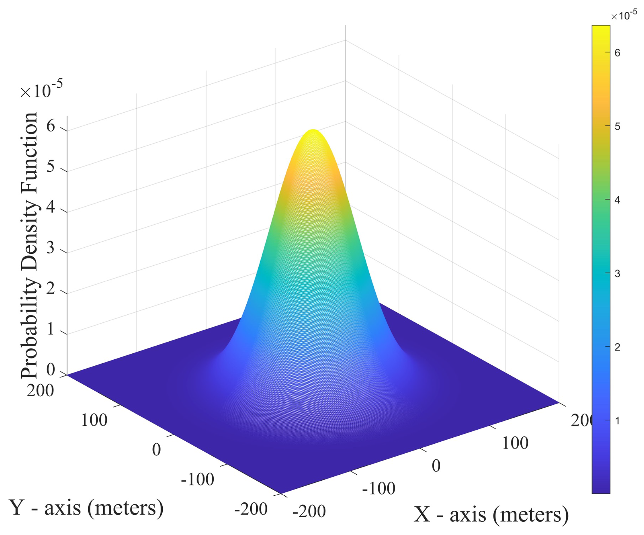
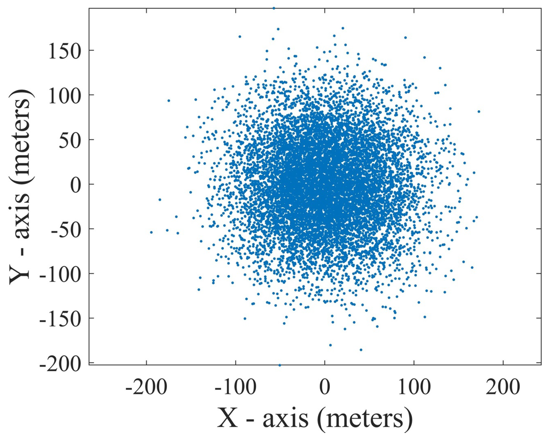
Equation (2) provides the probability density function of the target position in the x−axis and y−axis directions. In the following simulation study, we set the variance to 2500, indicating that the standard deviation of error dispersion is 50 m, which is consistent with the assumption scenario of ‘superposition of small disturbances’.

B.

Target Motion Model

This section uses Markov chain models to model the target motion characteristics. By guiding Monte Carlo sampling through target motion state transition rules, the target motion patterns are constrained to concentrate the sample space in high-probability motion pattern regions, avoiding redundant calculations of low-probability paths in Monte Carlo random sampling. On this basis, the influence of sensor measurement error is considered, which better simulates the actual working state of the sonar and improves the authenticity of the evaluation results.

The Markov chain model guides Monte Carlo sampling through state transition probabilities. In the Markov chain modeling process, we fully consider the target motion law, so the generated target motion trajectory is more realistic and reliable. With the target motion trajectory and sonar search path, the relative situation at different time points becomes a known quantity, and the detection probability can be solved based on the sonar equation. Therefore, in the Markov chain model, different state transition probabilities result in different probabilities of the target moving in different directions, leading to different generated target motion trajectories and ultimately resulting in different target detection probabilities.

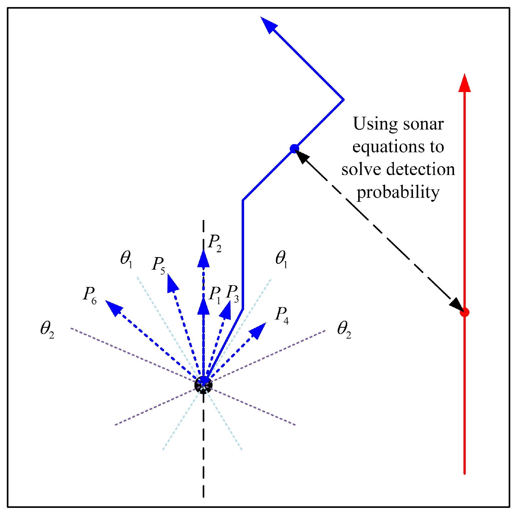
When modeling target motion via the Markov process, it is assumed that the target heading state transition rule is as follows: (1) The probability that the target maintains its original heading is A. (2) The probability of target turning is $1-A$. When the target turns, the probability of turning at a small angle ($0\sim {\theta }_1$) is B, and the probability of turning at a large angle (${\theta }_1\sim {\theta }_2$) is $1-B$. Among them, if the target turns at a small angle, the heading is taken randomly between $0\sim {\theta }_1$, and the same applies to the turns at a large angle. The transition rule for the state of the target velocity is as follows: (1) The probability that the target velocity remains unchanged is C. (2) The probability of a change in the velocity of the target is $1-C$. If the target velocity changes, the velocity is randomly selected between $\left[{\nu }_{min},{\nu }_{max}\right]$. In practical applications, we use the random number generator rand function in MATLAB R2020b to randomly select values, and set the convergence standard according to the number of simulations. We set the Monte Carlo number to 10,000 and stop running when the maximum number of simulations is reached. Therefore, the transition probabilities of the target motion state can be expressed as the following six types and satisfy $P_1+P_2+P_3+P_4+P_5+P_6=1$.

(1) The probability that the target heading and velocity remain unchanged is $P_1=AC$.

(2) The probability of the target heading remaining unchanged and the velocity changing is $P_2=A(1-C)$.

(3) The probability of turning at a small angle without changing the target velocity is $P_3=(1-A)BC$.

(4) The probability of turning at a large angle without changing the target velocity is $P_4=(1-A)(1-B)C$.

(5) The probability of a small angle turn with a change in target velocity is $P_5=(1-A)B(1-C)$.

(6) The probability of a large angle turn with a change in the target velocity is $P_6=(1-A)(1-B)(1-C)$.

According to the above modeling, the schematic diagram of target motion state transition and trajectory generation based on Markov model optimization is shown in Figure 1.

Figure 1 fully illustrates how the Markov chain state transition probability guides the motion of the target, and the next motion state of the target is calculated based on the state transition probabilities in different directions. The length of the blue dashed line in Figure 1 represents the current movement distance in the next time interval. At a certain moment, the target is at the blue dot position and the sonar is at the red dot position. At this time, the relative position between the sonar and the target is determined, and the detection probability can be obtained by solving the sonar equation.

When the target position obtained via the Markov process is the coordinate origin, assuming that X and Y follow a normal distribution with a mean of 0 and a variance of 2500, the joint probability density function of the sensor observation position is shown in Figure 2, and the possible distribution of observation position points is shown in Figure 3.

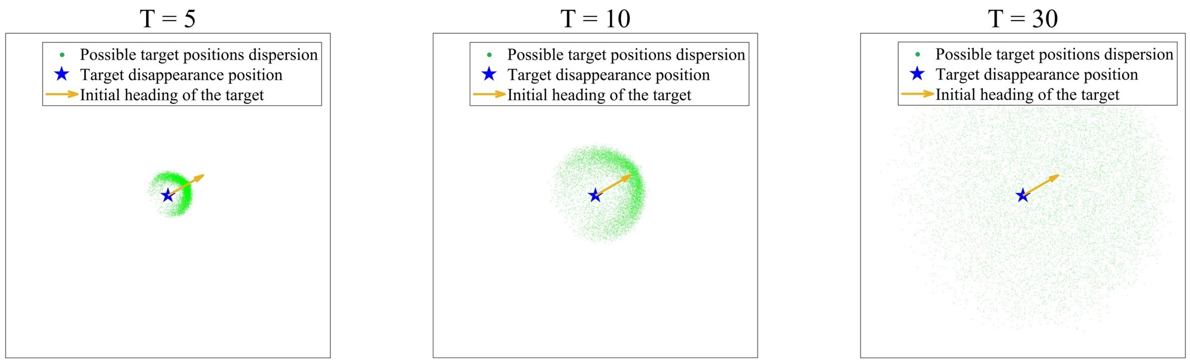
After the initial motion information of the target is given, Figure 4 shows the distribution of possible observed positions of the target at three time points of $T=5,10,30$, with the x-axis and y-axis values in the same range.

3.2. A Sonar Detection Performance Model Based on Spatiotemporal Discretization

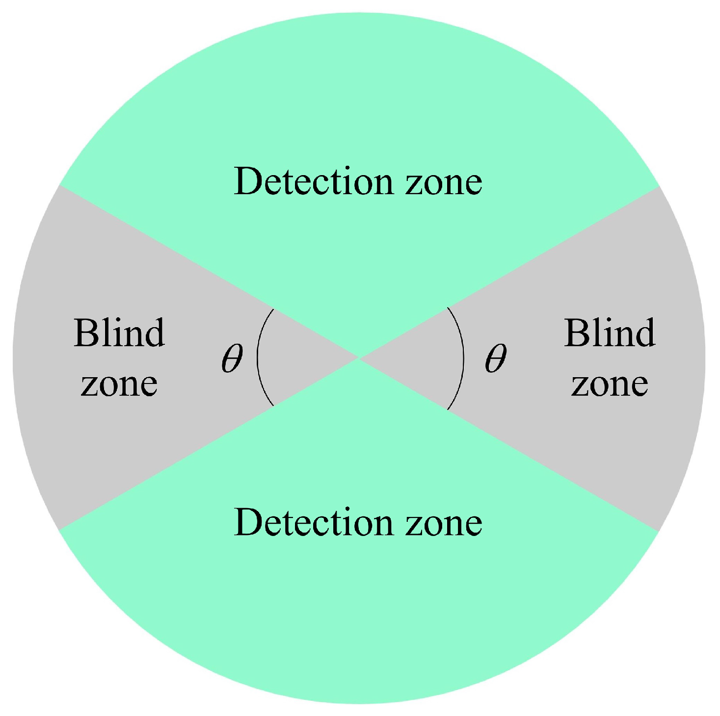
In practical operating environments, we assume sonar is limited by the beamforming characteristics of the sensor array, and there are common acoustic detection blind zones in the front and rear directions [33,34], as shown in Figure 5.

The calculation of sonar detection probability requires comprehensive consideration of multiple parameters such as environmental background noise, target radiation noise, and target sound scattering characteristics. Based on the sonar equation, the quantitative representation of the detection probability is achieved by calculating the signal excess, and its mathematical expression is as follows [35]:

$$\left\{\begin{array}{c}SNR={\displaystyle \frac{lg{P}_f}{lgP{d}_i}}-1\hfill \\ P{d}_i={10}^{{\displaystyle \frac{lg{P}_f}{(SN{R}_{0.5}\times {10}^{0.1\times SE}+1)}}}\hfill \end{array}\right.$$

(3)

Equation (3) provides a method for solving the detection probability, where $P_f$ represents the false alarm probability, usually taken as ${10}^{-4}$, and $SN{R}_{0.5}$ is the signal-to-noise ratio obtained when $P{d}_i$ equals 0.5. $SE$ represents the signal excess, which can be calculated using the sonar equation.

In the passive working mode of sonar [36,37], when noise is the main interference type, the signal excess is expressed as $SE=SL-TL-NL-DT+DI$, where $SL$ represents the target radiation sound source level, $TL$ represents the transmission loss between the target and the receiver, $NL$ represents the marine environmental noise level, $DT$ represents the sonar detection threshold, and $DI$ represents the receiving directionality index. Among them, $TL$ is calculated according to the empirical equation $20lgr+\alpha ·r$, where r represents the distance between the target and the receiver, $\alpha$ represents the attenuation coefficient, and its relationship with frequency is expressed as follows [38]: $\alpha ={\displaystyle \frac{0.1f^2}{1+f^2}}+{\displaystyle \frac{40f^2}{4100+f^2}}+2.75\times {10}^{-4}{f}^2+0.003$.

In the active working mode of sonar [36,37,39], when noise is the main type of interference, the signal excess is expressed as $SE=S{L}_1-2TL+TS-NL-DT+DI$. Here, $S{L}_1$ represents the emission sound source level, $TS$ represents the target strength, which is strongly correlated with the real-time situation and is constantly changing. The meanings of the other parameters are the same as those in the previous text.

The detection probability only characterizes the detection efficiency of sonar at a specific time point, while the cumulative detection probability [40], as a time series analysis method based on probability theory, can more comprehensively reflect the comprehensive performance of sonar systems by dynamically integrating the detection efficiency at various time points throughout the entire process. Owing to the certain correlation between the two detection results with a small time interval, the $(\lambda ,\sigma )$ process model considering temporal correlation is used to solve the cumulative detection probability. The mathematical expression is as follows [41]:

$$CD{P}_i=1-{\displaystyle \frac{1-max\left(P{d}_i\right)}{1-\beta ·max\left(P{d}_i\right)}}\prod _{i=1}^N(1-\beta ·P{d}_i)$$

(4)

Equation (4) provides a method for solving the cumulative detection probability, where $P{d}_i$ represents the instantaneous detection probability corresponding to n time points, $max\left(P{d}_i\right)$ represents the maximum value of $P{d}_i$, $\beta =1-exp(1-\lambda \Delta )$, $\Delta$ represents the sonar detection time interval, and $\lambda$ represents the signal jump rate.

3.3. Efficiency Evaluation Model Based on Multidimensional Indicators

In the actual sonar search scene, traditional detection probability estimation values often fall into the dilemma of ‘achieving laboratory accuracy and prioritizing actual efficiency’ because they ignore the uncertainty of the target spatial distribution. We introduce the effective detection rate as an evaluation indicator, achieving a leap from ‘single point detection efficiency’ to ‘regional control capability’. This indicator not only integrates physical characteristics such as sonar equation and transmission loss models, but also converts complex underwater acoustic physical models into decision-making languages through the ‘detection threshold’.

During the target search process, factors such as uncertainty in target location and blind zone in sonar detection may lead to extreme values in detection efficiency. These extreme values are not data anomalies, but rather reflections of the boundary characteristics of sonar detection efficiency in the practical scene. As a robust statistic, the interquartile range (IQR) can stably reflect the fluctuation characteristics of the detection interval by measuring the middle $50\%$ range of the data distribution, avoiding evaluation distortion caused by extreme value interference and being more in line with the practical application scene. Variance quantifies the degree of data dispersion and is suitable for evaluating the overall volatility of core indicators such as detection probability. It can effectively reveal the systematic influence of uncertainty factors on sensor detection efficiency. Confidence analysis can provide the credibility of sonar detection efficiency evaluation results, achieving a leap from ‘point estimation’ to ‘interval estimation’. In order to characterize the effective detection capability of sonar systems for targets at different discrete time points, an evaluation index of the ‘effective detection rate’ is designed. By setting a certain ‘detection threshold’, the effective detection capability of sonar systems at different time points can be quantitatively expressed, avoiding misleading the overall evaluation by local high-probability areas.

Taking into account the above evaluation indicators, we can effectively compensate for the limitation of a single estimated value not reflecting the possible value distribution. Therefore, the multidimensional statistical index analysis introduced in this paper includes detection probability estimation, cumulative detection probability estimation, effective detection rate calculation, volatility analysis (including quartile range analysis and variance calculation), and confidence analysis. A sonar detection efficiency evaluation index system is constructed from multiple dimensions such as anti-interference and credibility. We introduce multidimensional statistical indicators to quantify detection efficiency at a certain point in time, and use uncertainty quantification analysis instead of single estimation analysis, which provides more comprehensive information for evaluating sonar detection efficiency and helps decision-makers better understand the risks of search schemes.

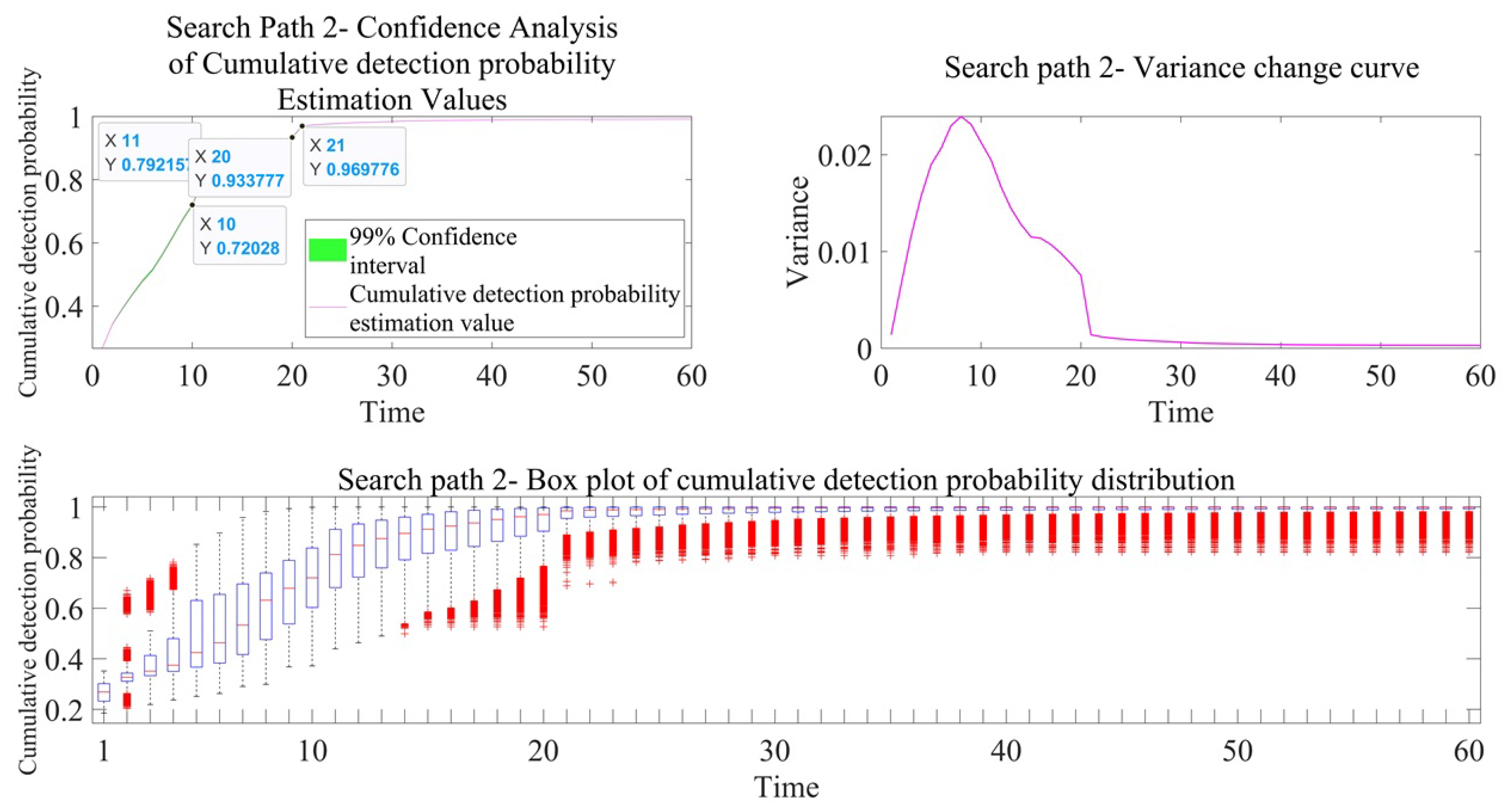
For a certain point in time, multiple Monte Carlo processes will obtain multiple detection probability values and multiple cumulative detection probability values. The minimum mean square error method is used to estimate the detection probability and cumulative detection probability values. Assuming that the detection probability and cumulative detection probability corresponding to a certain time point are $P{d}_1,P{d}_2,P{d}_3,\dots ,P{d}_N$ and $CD{P}_1,CD{P}_2,CD{P}_3,\dots ,CD{P}_N$, respectively, we get the corresponding values of $Pd$ and $CDP$ when $min\left(\sqrt{{\sum }_{i=1}^N{(P{d}_i-\overline{Pd})}^2}\right)$ and $min\left(\sqrt{{\sum }_{i=1}^N{(CD{P}_i-\overline{CDP})}^2}\right)$, and use them as the estimated values of the detection probability and cumulative detection probability.

By statistically analyzing the multiple detection probability values mentioned above, and using detection probability values greater than or equal to $\omega$ as effective probability values, the effective detection rate $P_e$ can be obtained, which can intuitively quantify the overall effectiveness of sonar systems in detecting targets in complex environments. Equation (5) provides a method for solving the effective detection rate. Therein, $\omega \in \left[0,1\right]$.

$$\left\{\begin{array}{c}{P}_e={\displaystyle \frac{1}{N}}{\sum }_{i=1}^{N}f\left(P{d}_i\right)\hfill \\ f\left(P{d}_i\right)=\left\{\begin{array}{cc}1,\hfill & P{d}_i\ge \omega \hfill \\ 0,\hfill & P{d}_i<\omega \hfill \end{array}\right.\hfill \end{array}\right.$$

(5)

We perform data volatility analysis on the multiple detection probability values and cumulative detection probability values mentioned above, use the quartile range analysis method to determine the intervals $I_{Pd}$ and $I_{CDP}$ occupied by the middle 50% of the data, and calculate the variances ${{\epsilon }_{Pd}}^2$ and ${{\epsilon }_{CDP}}^2$ to quantify the data dispersion at that time point. When there is skewness in the data distribution, the interquartile range (25–75% interval) better reflects the fluctuation characteristics of the data subject than the variance, avoids extreme value interference, and characterizes the stable range of detection efficiency. Equation (6) provides a method for solving the interquartile range. Equation (7) provides a method for solving the variance.

$$\left\{\begin{array}{c}{I}_{Pd}\in [Q_{1\_Pd},Q_{3\_Pd}]=[\mathrm{quantile}(P{d}_i,0.25),\mathrm{quantile}(P{d}_i,0.75)]\hfill \\ I_{CDP}\in [Q_{1\_CDP},Q_{3\_CDP}]=[\mathrm{quantile}(CD{P}_i,0.25),\mathrm{quantile}(CD{P}_i,0.75)]\hfill \end{array}\right.$$

(6)

$$\left\{\begin{array}{c}{{\epsilon }_{Pd}}^2={\displaystyle \frac{1}{N-1}}{\sum }_{i=1}^N{(P{d}_i-Pd)}^2\hfill \\ {{\epsilon }_{CDP}}^2={\displaystyle \frac{1}{N-1}}{\sum }_{i=1}^N{(CD{P}_i-CDP)}^2\hfill \end{array}\right.$$

(7)

We conduct confidence analysis on the estimated values of multiple detection probability values and cumulative detection probability values mentioned above, converting the uncertainty of the estimated values into interval ranges in a probabilistic sense, and quantifying the 99% confidence interval of the estimated values. Through confidence analysis, the fluctuation range of the estimated value can be quantified.

We use statistical theory knowledge to quantitatively analyze data uncertainty, which avoids the extreme risks that a single estimate may bring and provides decision-makers with a complete information chain from ‘point estimation’ to ‘interval estimation’.

When using multidimensional indicator evaluation methods to evaluate sonar detection efficiency, we can obtain the effective detection rate, estimated detection probability, estimated cumulative detection probability, and their corresponding data volatility analysis confidence analysis results. When decision-makers need to compare the detection efficiency of two search paths and draw a conclusion on which one is better or worse, first of all, the detection probability is the most important. Whichever has a higher detection probability will have better detection performance. However, in practical situations, the detection probability is a variable over time, and we cannot judge the quality of the corresponding path based on the detection probability value at a certain point in time. Therefore, the cumulative detection probability index has certain advantages, but it is also a variable over time, and sometimes there may be situations where the cumulative detection probability curves of two search paths are roughly the same. In this case, we need to increase the judgment basis and compare the results of data volatility analysis and confidence analysis. When the data volatility of a certain search path is small (in quartile range analysis, the smaller the box length and variance of the middle $50\%$ of the data, the better the quality of the search path) and the confidence interval is small, it indicates that the quality of the search path is better.

If we use the proposed multidimensional evaluation method to determine the effectiveness of search path detection, the key lies in how to fully utilize and analyze the relevant detection probability data obtained to draw effective conclusions. Obtaining data through simulation can also provide powerful explanations for how decision-makers can use this indicator system. From this perspective, the effectiveness of using simulation data to support the proposed method is equivalent to using measured data.

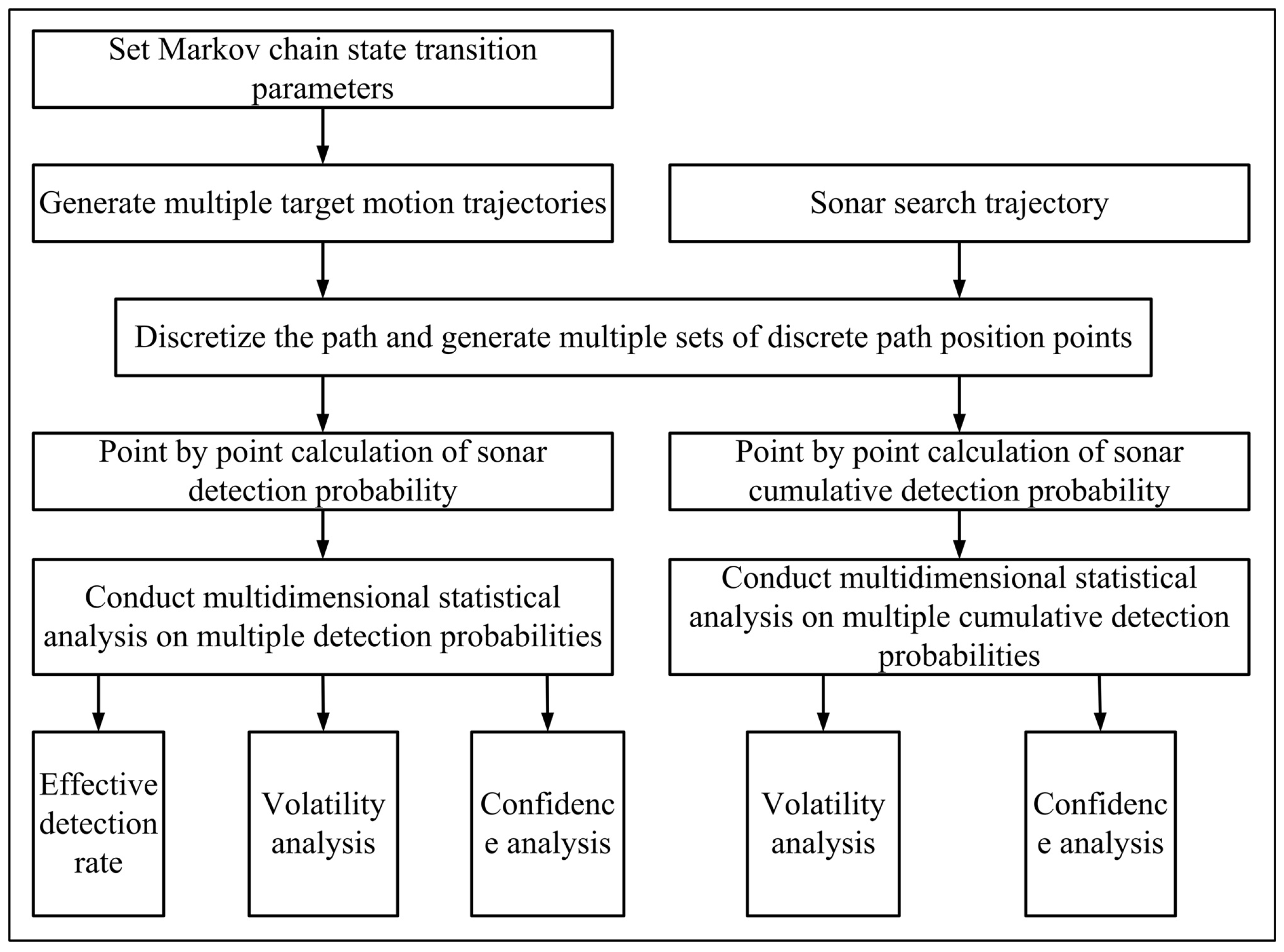
Based on the above content, a schematic diagram of the sonar search path detection efficiency evaluation model is shown in Figure 6.

In the process of solving the established model, the detection probability is mainly calculated based on the sonar equation, and then relevant statistical analysis is carried out on the detection probability data. Therefore, calculating the detection probability is the most fundamental and important step, and the parameters of the sonar equation in the model can be adjusted according to the actual situation. The changes in factors such as different sonar types and environmental conditions will ultimately be reflected in the changes of relevant parameters in the sonar equation. Therefore, this model is applicable to changes in external factors such as different sonar types and environmental conditions.

4. Numerical Results and Analysis

4.1. Numerical Simulation Calculation

The computer hardware configuration used for our simulation was the 11th Gen Intel (R) Core (TM) i7-11800H @ 2.30 GHz, and the software environment was MATLAB R2020b.

This section distinguishes between the active and passive working modes of sonar and uses multidimensional efficiency evaluation indicators as the driving force to conduct a detailed evaluation of the sonar search path detection efficiency, while conducting a simulation analysis and providing discussion. The simulation parameters are as follows: the probability of target turning is $1-A=50\%$, when the target turns, the probability of small angle turning (0∼${45}^{\circ }$) is $B=60\%$, and the probability of large angle turning (45∼${90}^{\circ }$) is $1-B=40\%$. The probability that the target velocity changes is $1-C=50\%$. The detection threshold $\omega =0.5$ is used to calculate the effective detection rate. The sensor observation error follows a normal distribution, $\delta =50$. It is well-known that the frequency band of radiated noise varies for different targets. In the simulation experiment of this paper, we are only concerned with the source level of the target according to the sonar equation, so we did not refine it to the frequency level. From the perspective of the efficiency evaluation model, this is reasonable.

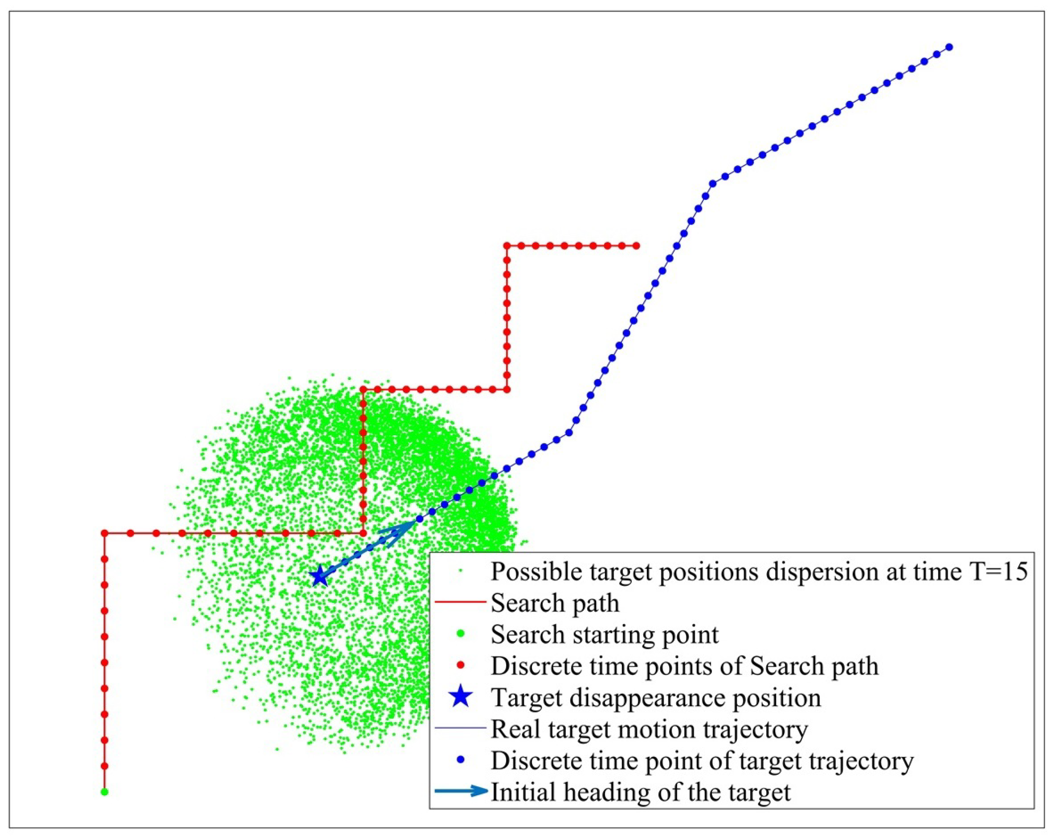
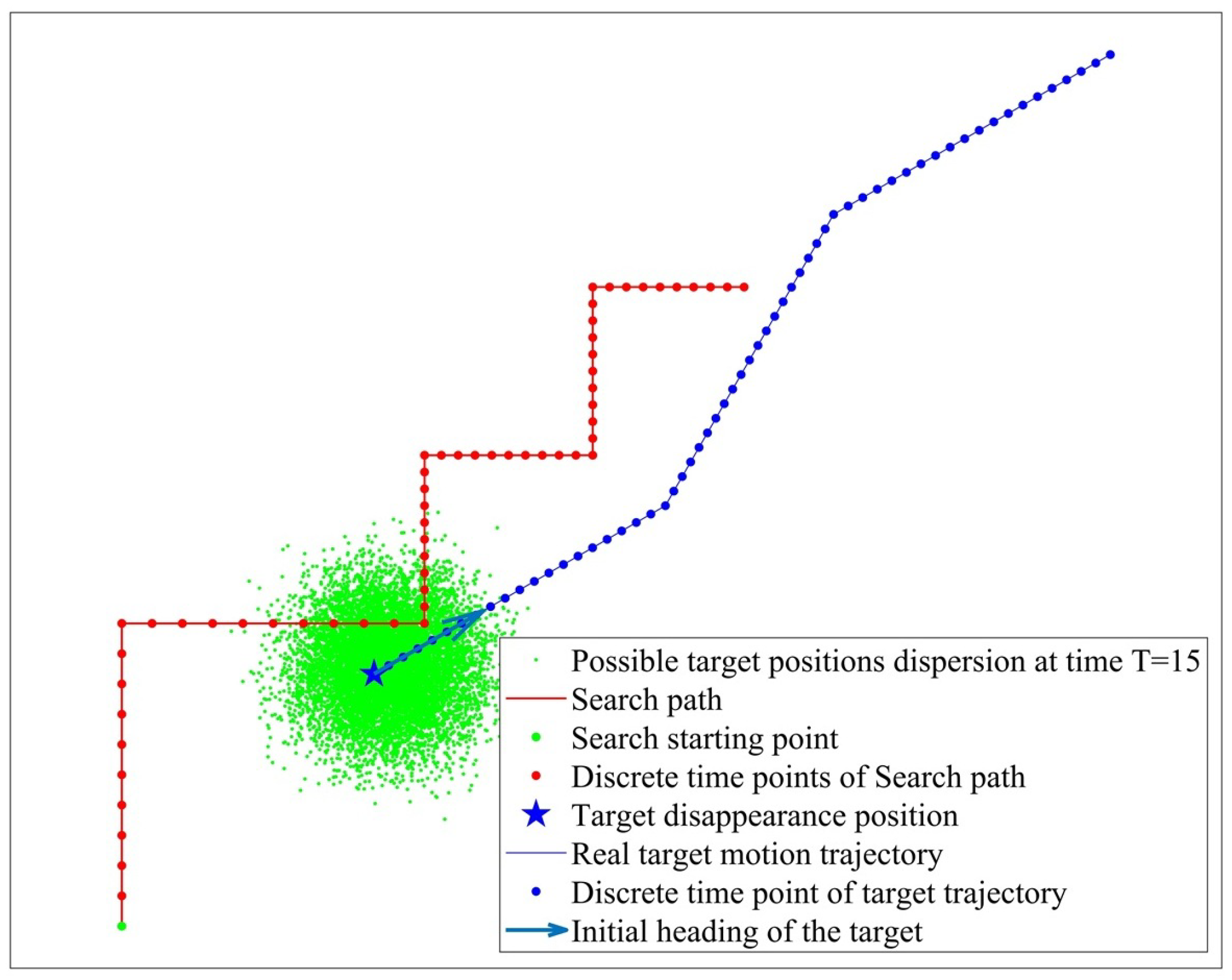
In order to verify the effectiveness of Monte Carlo sampling guided by the Markov chain model, we assume a real target trajectory and construct a target motion trajectory database via the Monte Carlo random sampling method and the Markov chain model-guided Monte Carlo sampling method. The evaluation results of the two target motion trajectories are compared and analyzed with the detection efficiency evaluation results of the real trajectory. Among them, during Monte Carlo random sampling, the next heading and velocity of target are randomly selected between 0∼${360}^{\circ }$ and $\left[{\nu }_{min},{\nu }_{max}\right]$. Furthermore, ${\nu }_{min}$ and ${\nu }_{max}$ are 180 m/min and 220 m/min, respectively. The sonar search path, the real target motion trajectory, and the possible target position distribution at T = 15 under the two sampling methods are shown in Figure 7 and Figure 8, respectively. By analyzing Figure 7 and Figure 8, it can be concluded that, taking into account the target motion pattern, Monte Carlo sampling guided by Markov chains can obtain more accurate target position dispersion.

The working process of sonar mainly relies on the sonar equation to solve the target detection probability, so changes in the relevant parameters of the sonar equation will seriously affect the accuracy of the detection probability. Among them, the target radiation sound source level SL will increase with the increase in target motion speed, the directivity index DI and detection threshold DT are related to the performance of the sonar itself, the background noise NL of the marine environment is related to the sea state, and the target reflection intensity TS is related to the real-time relative situation between the sonar and the target. Changes in these parameters cause changes in signal excess, which in turn leads to changes in detection probability.

In the simulation study of this article, we assume that the sonar working environment is stable, which means that parameters such as the ocean background noise (NL), detection threshold (DT), and directivity index (DI) remain unchanged. We assume that the propagation loss (TL) is calculated according to an empirical equation.

In the passive working mode of sonar, we assume that the radiated noise of the target will vary with the movement speed of the target. We define $FOM1=SL-NL+DI-DT$ and set it as a variable parameter value. The reason why it is a variable range is because we consider the influence of target motion speed on its radiated noise level SL.

In the active working mode of sonar, the sonar equation also includes the parameter of target reflection intensity, TS, which varies with the relative heading angle between the sonar and the target. We define $FOM2=S{L}_1-NL+DI-DT+TS$ and set it as a variable parameter value. The reason why it is a variable range is because we consider the influence of relative heading angle on target reflection intensity, TS.

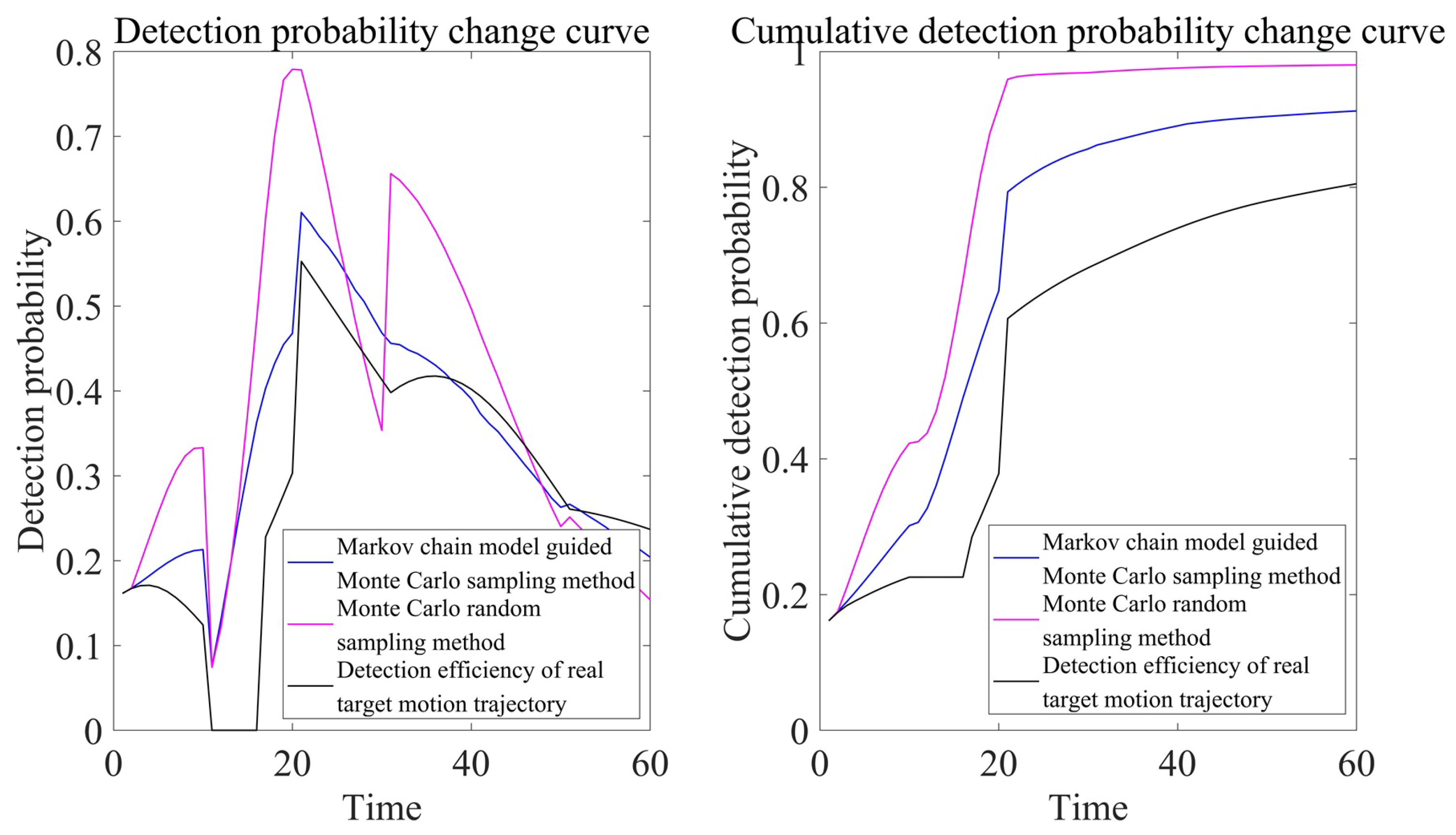
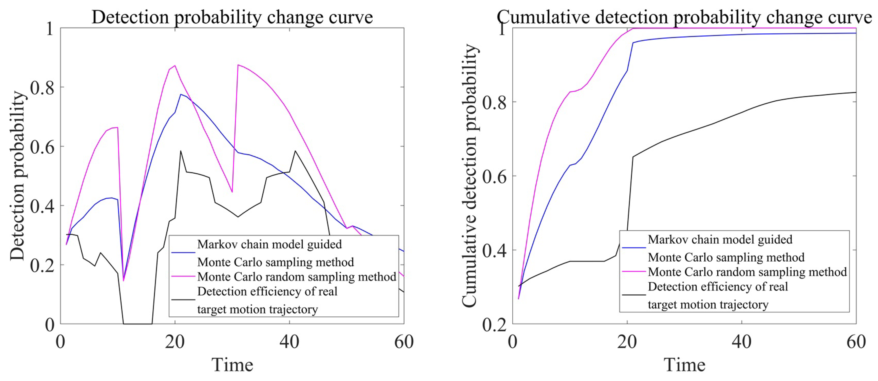
Under the active and passive working modes of sonar, the detection efficiency evaluation results of the two sampling methods and the real target motion trajectory are shown in Figure 9 and Figure 10, respectively.

By analyzing Figure 9 and Figure 10, it can be observed that the target motion trajectory database generated during Monte Carlo sampling guided by the Markov chain model is more accurate, whether in the active or passive working mode of sonar. The efficiency evaluation index results are closer to those of the real target motion trajectory. This indicates that using Markov chain models to guide Monte Carlo sampling can more effectively capture the uncertainty of target motion, verifying the effectiveness of this method.

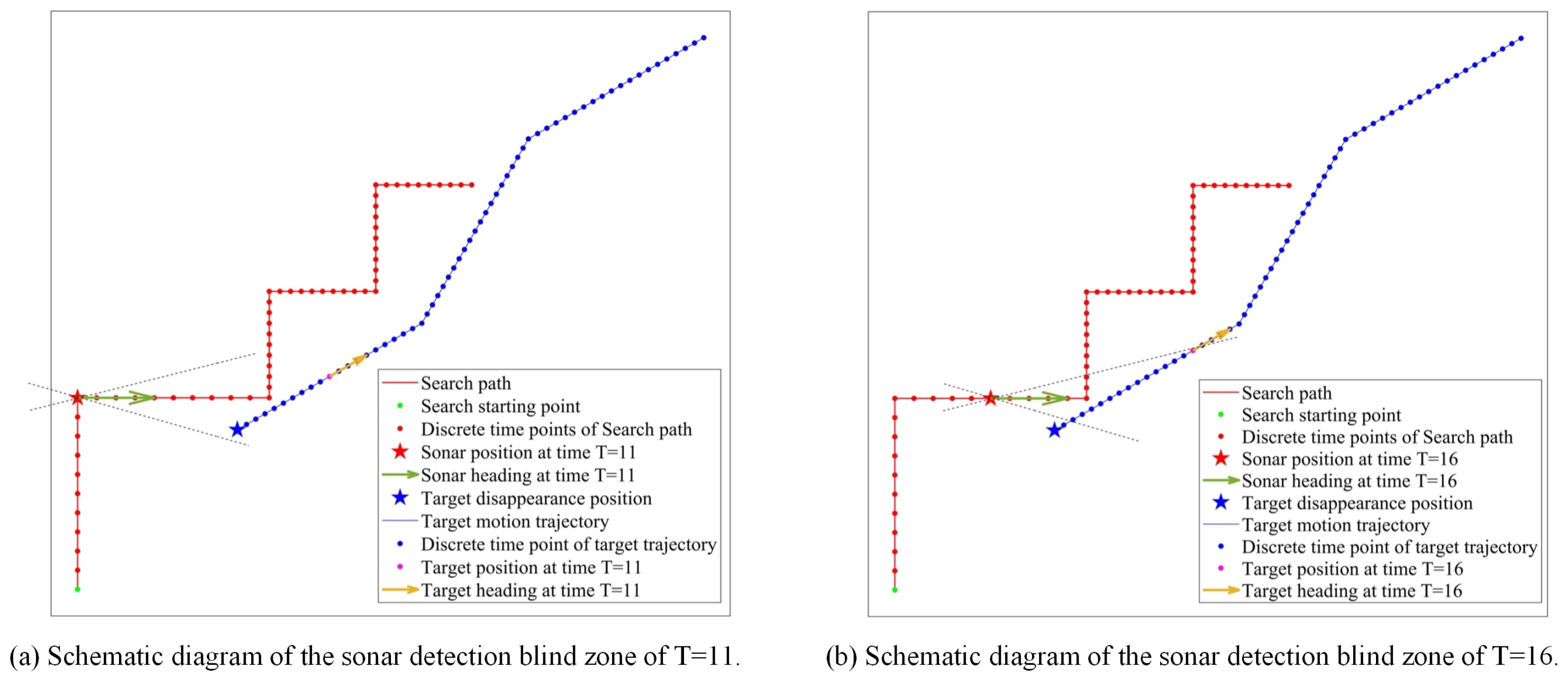
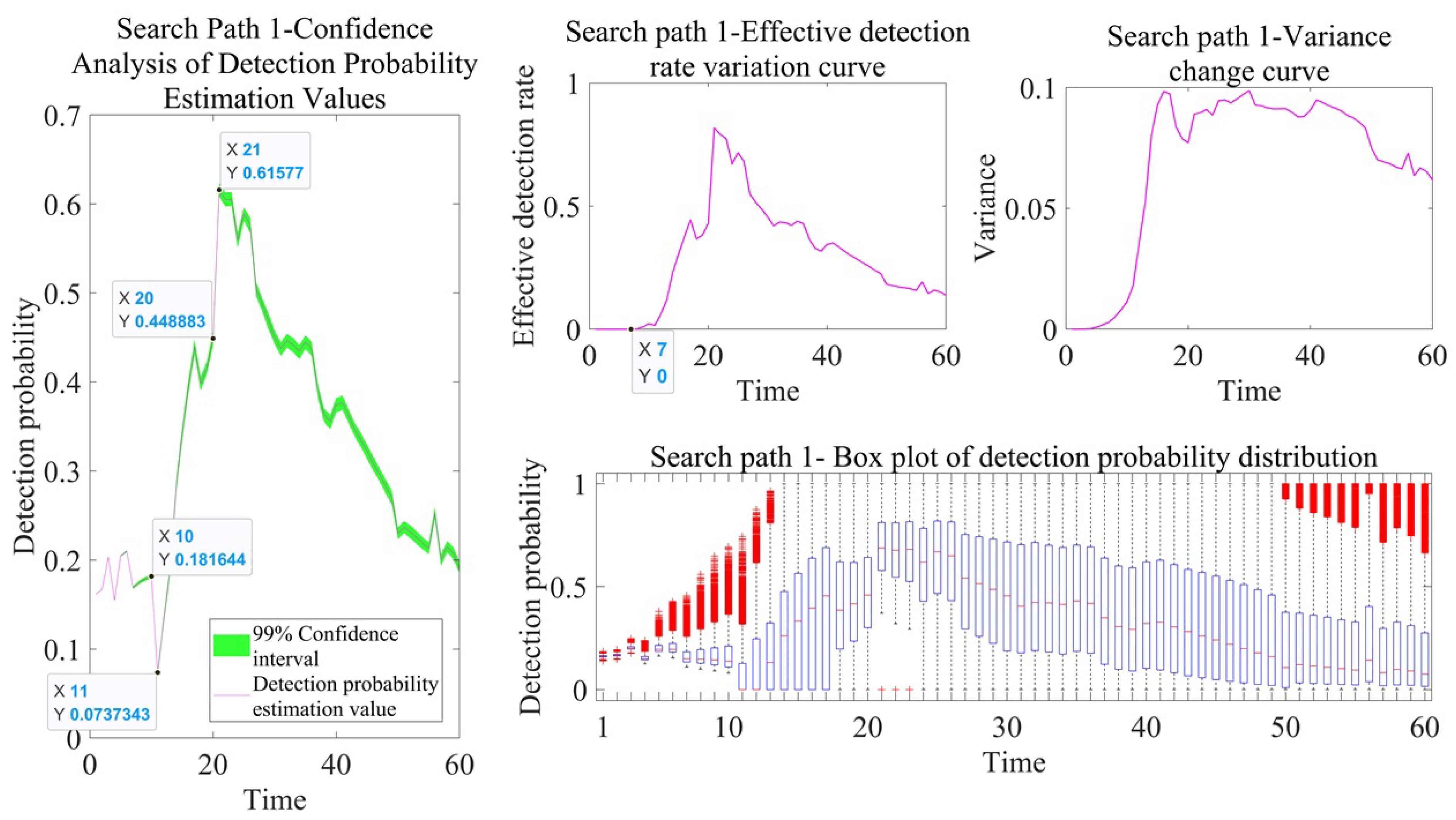
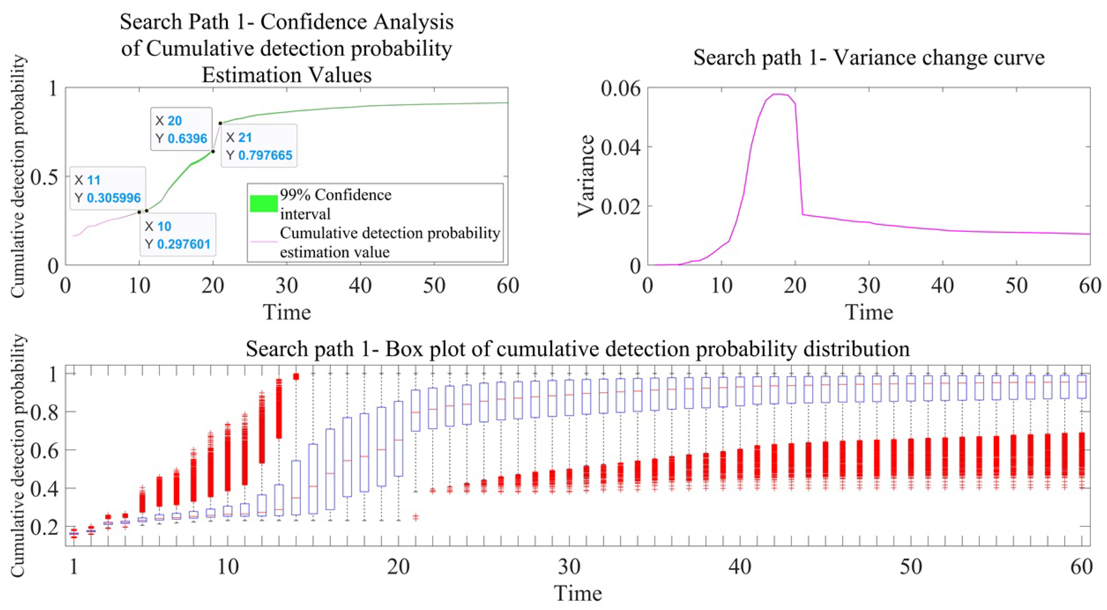
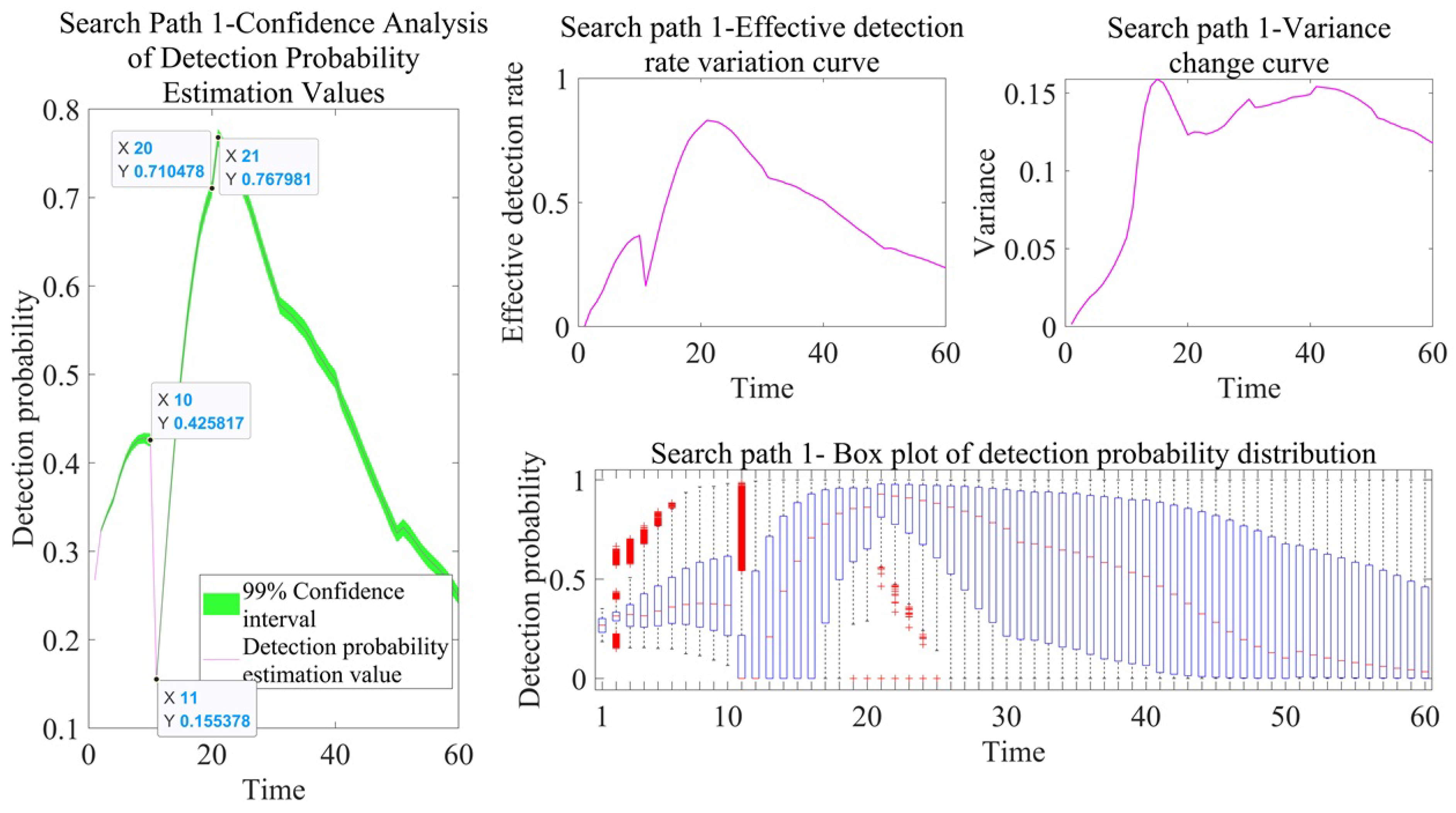
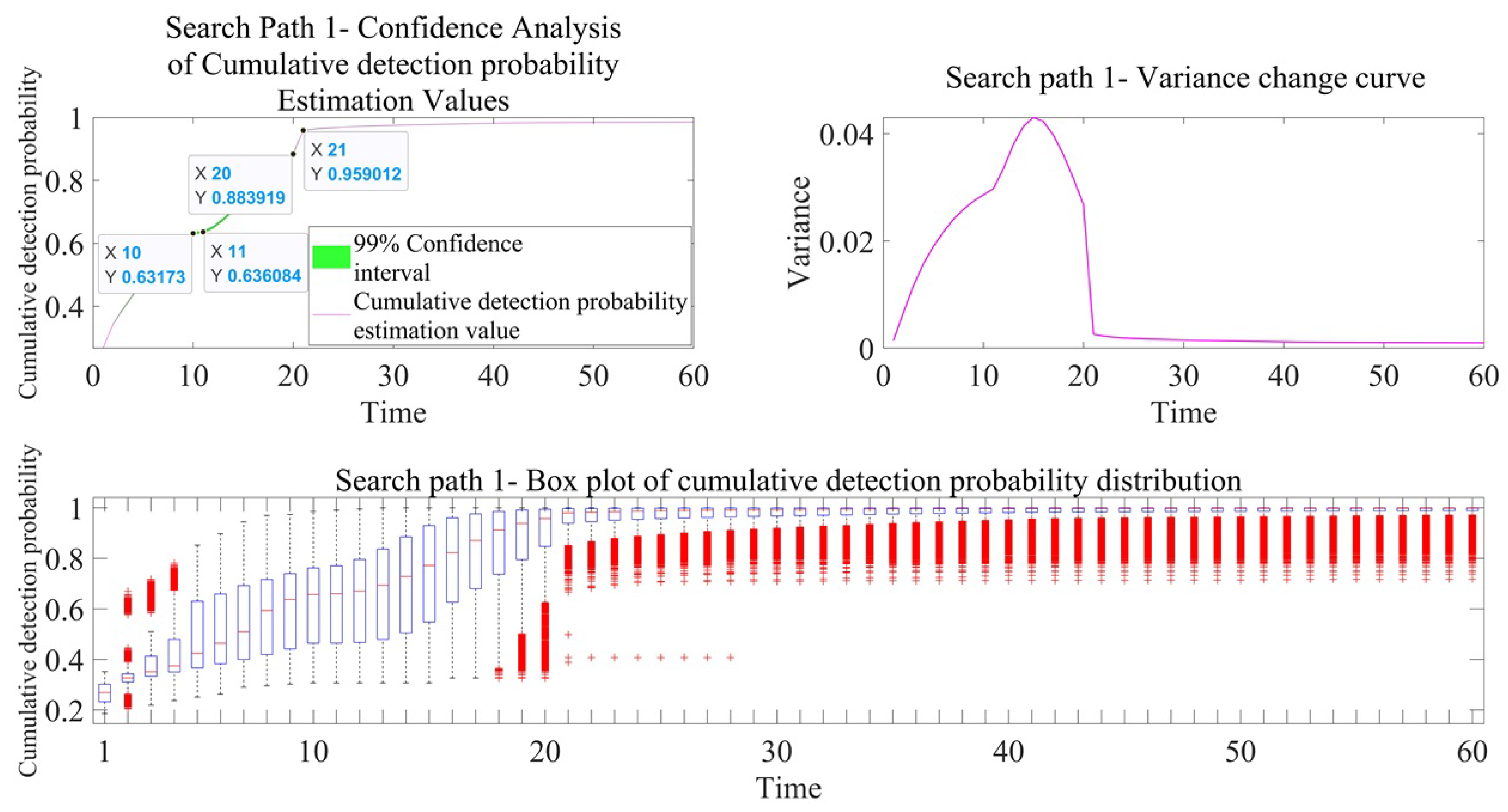
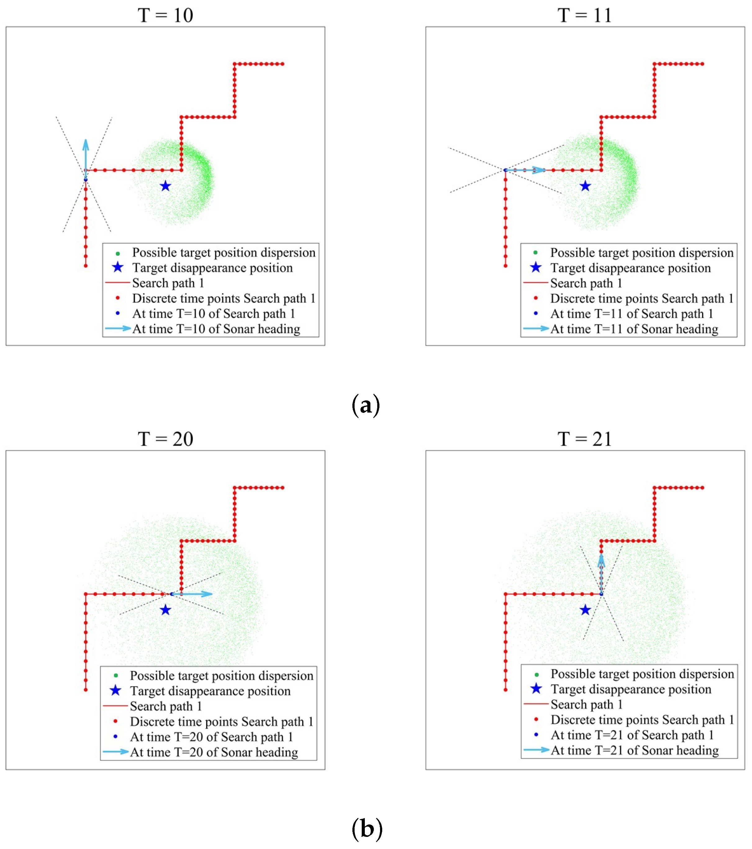
We analyzed the efficiency evaluation results of the real target motion trajectory and found that there was a sudden drop phenomenon between T = 10 and T = 11, which was related to the sonar detection blind zone. During the time period from T = 11 to T = 16, the detection probability remained 0, because the target was always within the detection blind zone range of sonar, as shown in Figure 11.

At different discrete time points, the target has multiple possible positions—that is, there are multiple detection probabilities. Since the process of solving the detection probability using sonar equations is independent when the target is in different positions, we assume that multiple detection probability data at the same discrete time point have strict independence, which meets the requirements for conducting estimation analysis, quartile range analysis, variance analysis, and confidence analysis.

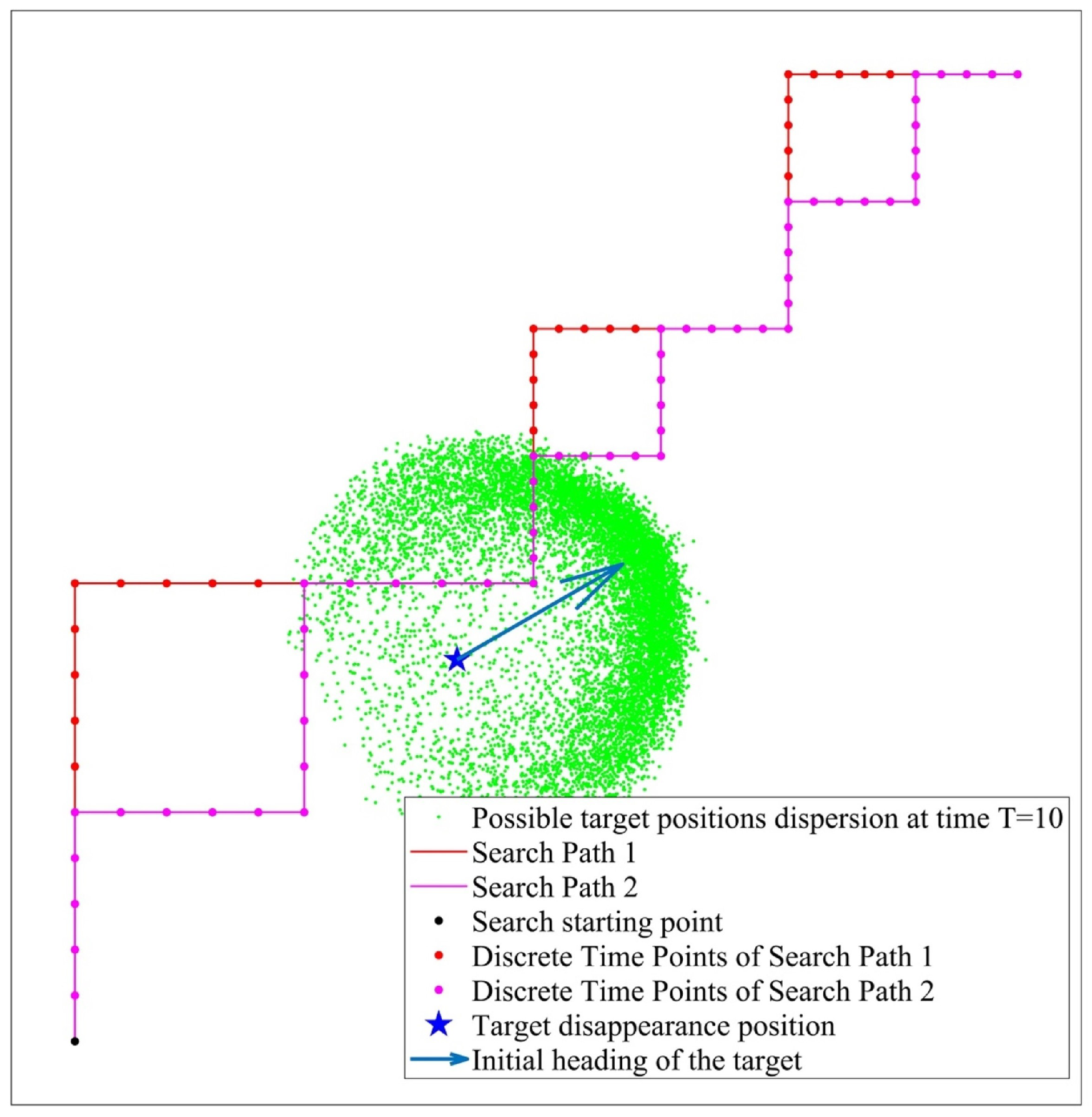
In order to demonstrate the role of multidimensional statistical index analysis, we set up two sonar search trajectories and construct a target motion trajectory database based on Markov chain model-guided Monte Carlo sampling. Figure 12 shows the relative situation between two sonar trajectories and the possible distribution of target positions at time T = 10.

The detection efficiency evaluation results of two search paths for targets under the passive working mode of sonar are shown in Figure 13, Figure 14, Figure 15 and Figure 16.

The detection efficiency evaluation results of two search paths for targets under the active working mode of sonar are shown in Figure 17, Figure 18, Figure 19 and Figure 20.

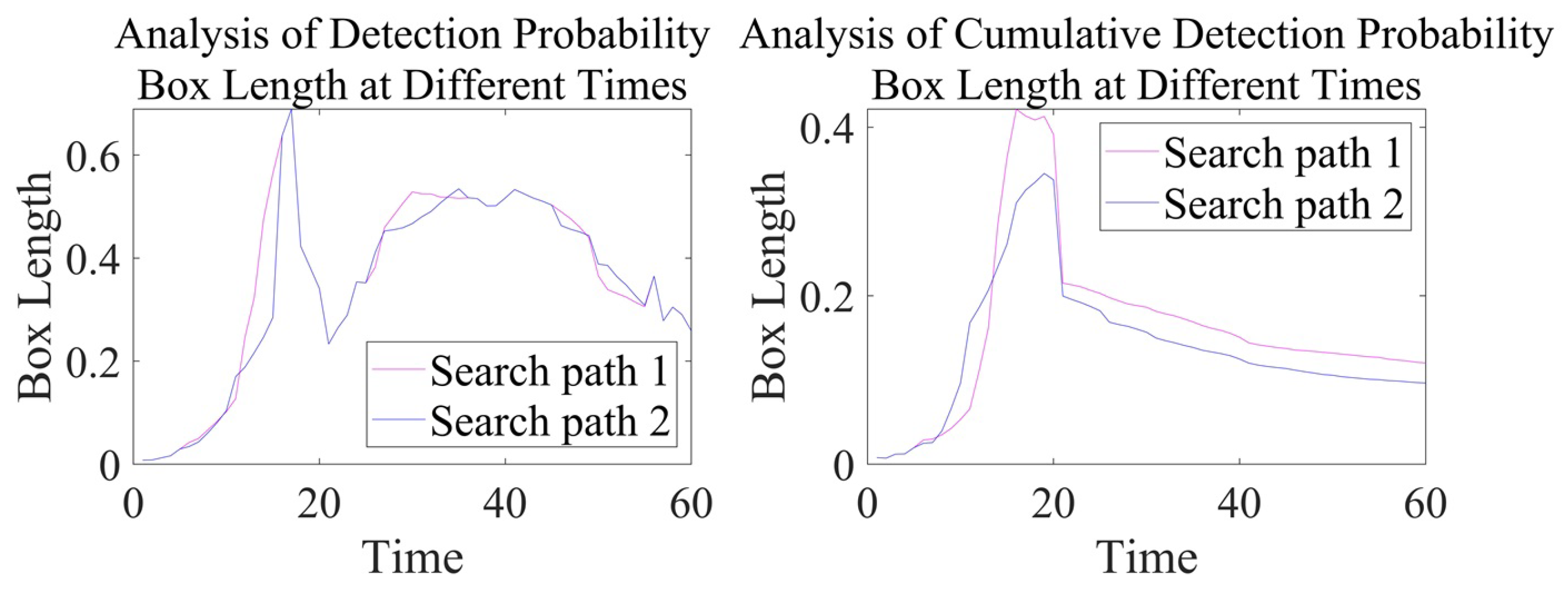
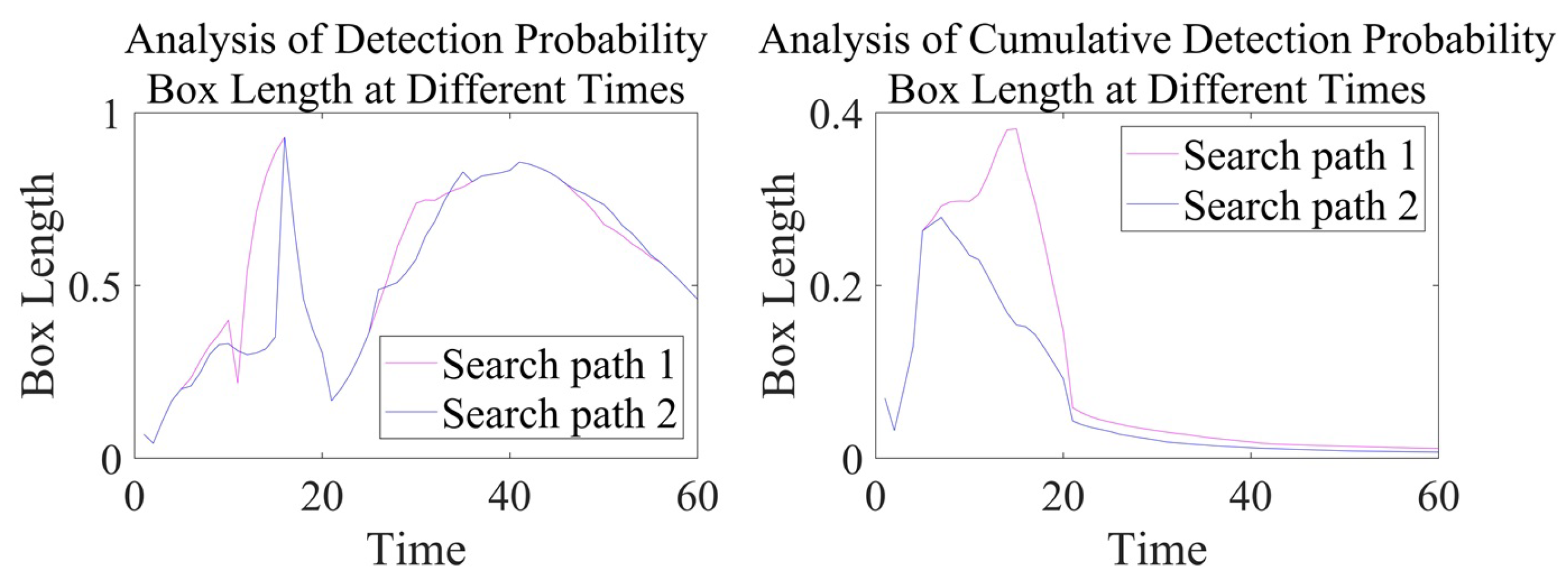
An analysis of the simulation results of the different sonar search path detection efficiency in both active and passive working modes reveals the following: (1) For the detection probability, the amplitude and trend of the estimated detection probability values for the two search paths are roughly similar. However, by analyzing the detection probability box plot, it can be concluded that in the passive and active working modes of sonar, during the time period from T = 11 to T = 15, the box length of path 2 is reduced by 0∼0.2 and 0∼0.5, respectively, compared to path 1, indicating that the data are concentrated in a narrower range and that the data dispersion is lower, reflecting the compactness and low volatility of the data distribution. (2) For the cumulative detection probability, the estimated amplitude and trend of the cumulative detection probability for the two search paths are roughly similar, making it difficult to distinguish the advantages and disadvantages of the two search paths. However, through data volatility analysis and quartile range analysis, it can be concluded that in the passive and active working modes of sonar, during the time period from T = 15 to T = 20, the box length of path 2 is reduced by 0∼0.1 and 0∼0.2, respectively, compared to path 1, and the variance is reduced by 0∼0.02 and 0∼0.03, respectively, compared to path 1. Similarly, this indicates that the distribution of cumulative detection probability data is more concentrated and that the degree of dispersion is lower. In order to quantify the advantages of box plot analysis, statistics were gathered on the box lengths at different times in the above box plot, as shown in Figure 21 and Figure 22.

Overall, at different time points, the data distribution corresponding to path 2 is more concentrated and stable. In order to more intuitively demonstrate the advantages of multidimensional evaluation methods, some key indicators are summarized in

Table 1. Key performance indicators of simulation results at time T = 30.

Sonar Working Mode	Sonar Search Path	$\mathit{CDP}$	99% Confidence Interval Length	Box Length	${\mathit{\epsilon }}_{\mathit{CDP}}^2$
Passive	Path 1	0.8611	0.0060	0.1863	0.0145
	Path 2	0.8841	0.0050	0.1566	0.0095
Active	Path 1	0.9751	0.0021	0.0320	0.0015
	Path 2	0.9839	0.0013	0.0208	0.0006

. Due to the fact that different discrete time points correspond to multiple detection probabilities and multiple cumulative detection probabilities, each discrete time point contains relevant multidimensional indicator analysis. Therefore, the data in Table 1 is the statistical analysis results of multidimensional indicators for a certain time point. In Section 3, we determined that since the detection probability is a variable over time, it is unreasonable to judge the quality of the corresponding path based on the detection probability value at a certain point in time. Therefore, Table 1 only provides the cumulative detection probability value, 99% confidence interval length, variance, and box length in the quartile range analysis at T = 30.

By analyzing the data in Table 1, we can conclude that regardless of whether the sonar is actively or passively working, the difference in cumulative detection probabilities between the two search paths is very small at T = 30. We cannot solely rely on cumulative detection probabilities to evaluate the quality of the two paths. With the assistance of variance and box length indicators, we can more confidently conclude that path 2 has better detection performance, which reflects the advantages of the constructed model.

4.2. Discussion on Numerical Simulation Results

(1)

Discussion on the Detection Probability Results

As time progresses, the estimated detection probability fluctuates up and down. The reason is that after spatiotemporal discretization, the velocity of the target at each time point is different, resulting in different radiation noise levels. In addition, the relative situation between the sonar and the target changes in real time, ultimately affecting the detection probability. For search path 1, there is a significant change in the estimated detection probability during the two time periods of T = 10 to T = 11 and T = 20 to T = 21. For search path 2, there is a significant change in the estimated detection probability during the three time periods of T = 10 to T = 11, T = 15 to T = 16, and T = 20 to T = 21. The reason is that in search path 1, the sonar turns at two time points T = 11 and T = 21, while in search path 2, the sonar turns at three time points, T = 11, T = 16, and T = 21. Owing to the influence of the blind zone in the detection of the head and tail, there is a significant change in the detection probability. The detection probability of other turning moments changes relatively little, because the possible target position distribution range is too small or too large. We provide an explanation for search path 1, as shown in Figure 23.

Before the time point of T = 21, the estimated detection probability showed an overall increasing trend, as the relative distance between the sonar and the possible target position gradually decreased, resulting in an increasing detection probability. After the time point T = 21, the estimated detection probability begins to decrease. This is because the possible target position dispersion area gradually expands outward, and the relative distance between the sonar and the target gradually increases, resulting in a gradual decrease in the detection probability.

(2)

Discussion on Cumulative Detection Probability Results

According to the calculation equation of the cumulative detection probability, it shows a trend of ‘only increasing without decreasing’. The change in detection probability is indirectly reflected in the cumulative detection probability change curve. For example, for search path 1, from time points T = 10 to T = 11, due to a significant decrease in the estimated detection probability, the growth rate of the cumulative detection probability decreases significantly, and even tends to flatten out. From time point T = 20 to T = 21, due to the significant increase in the estimated detection probability, the growth rate of the cumulative detection probability has improved. After the time point of T = 21, as time passes, the detection probabilities of the two search paths gradually decrease; therefore, the increasing trend of the cumulative detection probability tends to flatten out.

(3)

Discussion on Effective Detection Rate Results

As time progresses, the effective detection rate also constantly changes, and its changing trend is the same as that of the estimated detection probability. This is because we set the effective detection rate threshold to 0.5, and as the detection probability increases, the effective detection rate will inevitably increase accordingly. In the passive working mode of sonar, the effective detection rate remains at 0 until time point T = 8. This is because the sonar is relatively far from the possible target position, and the detection probability remains below 0.5. However, due to the strong detection capability of sonar in active working mode, there has been no situation where the effective detection rate is 0.

(4)

Discussion on Confidence Results

Figure 13, Figure 15, Figure 17, and Figure 19 show that the 99% confidence level of the estimated detection probability is relatively high. This indicates that the approach of using the minimum mean square error method to obtain estimates in this article is reasonable and reliable.

(5)

Discussion on the Results of Interquartile Range Analysis

Whether for the detection probability or the cumulative detection probability, the trend of the data distribution box plot is the same as the trend of the estimated value, but there are some outliers (red part in the figure). The outliers represent the extreme values of the detection probability caused by the uncertainty of the target position. Outliers with low detection probabilities are mostly distributed in the sonar detection blind zone, while outliers with high detection probabilities may be concentrated in the sonar detection advantage area. These outliers are not data anomalies, but rather a reflection of the boundary characteristics of sonar detection efficiency in the practical scene. There are two reasons for the occurrence of outliers: (1) It is related to the Tukey coefficient, which is taken as 1.5 in this paper. The larger the coefficient value, the stricter the outlier detection criteria and the larger the threshold range. (2) It is related to the distribution characteristics of the data itself.

(6)

Discussion on Variance Results

Whether for the detection probability or cumulative detection probability, the variation of variance is influenced by various factors such as the sonar blind zone position, the relative situation between the sonar and the target, and the possible target position dispersion range. It reflects the degree of data dispersion, and the variance size is proportional to the 99% confidence interval range of the corresponding estimated value.

(7)

Other Discussions

In the modeling process of Markov chain, we fully consider the target motion law, so the target generated by this model may have a more realistic and accurate position. In different target motion patterns, we can modify the target motion law during the Markov chain modeling process to correspond to the changing target motion patterns. In theory, we can still obtain a high-fidelity target motion trajectory library. In addition, the distribution of sensor measurement errors is added to the possible location points of the target, and different distributions of measurement errors will result in different final detection performances. However, under the condition of adding the same sensor measurement error distribution, the proposed Markov method still has certain advantages compared to traditional methods due to generating more realistic possible target location points. Overall, the constructed model is insensitive to different target motion patterns or sensor error distributions.

In reference [32], the author solved the signal excess based on the sonar equation, and then calculated the detection probability of the target. Essentially, it belongs to a single indicator evaluation method. When we need to compare the detection efficiency of two search paths and provide a conclusion on which one is better or worse, the proposed method can provide a more comprehensive and accurate comparison conclusion.

5. Conclusions

The underwater environment is complex and ever-changing, and the propagation of sound waves is easily affected by factors such as terrain and hydrological conditions. This makes the design and execution of the search path directly determine the success or failure of the detection task. Therefore, it is of great significance to carry out detection efficiency evaluation for sonar search paths. Through systematic performance evaluation, it is possible to quantitatively analyze the changes in the detection probability of specific path schemes for targets in specific environments. This can provide a scientific basis and decision support for optimizing search strategies, rationally allocating detection resources, and improving task success rates. We propose a method of discretizing trajectories and conducting point-by-point detection efficiency evaluation to address the problem of static modeling methods having difficulty handling the complex scene environment of real-time changes in relative situations during sonar search in existing effectiveness evaluation research. In response to the problem that traditional Monte Carlo random sampling strategies have difficulty accurately characterizing target motion patterns, leading to inaccurate performance evaluation, we optimize the Monte Carlo sampling strategy based on Markov models. We have developed a multidimensional efficiency evaluation index system to address the issue of a single evaluation dimension being unable to characterize the data distribution characteristics of efficiency indicators.

In summary, we have proposed a multidimensional comprehensive detection efficiency evaluation method for the sonar search path based on dynamic spatiotemporal interaction, which achieves a full-chain quantitative evaluation of ‘spatiotemporal discrete modeling–situational dynamic deduction–probability-based statistical analysis’. The proposed method overcomes the limitations of entire-path sonar detection efficiency evaluation and avoids the problem that a single evaluation index estimation value masks the data distribution characteristics. And we use the Monte Carlo optimization sampling strategy based on the Markov chain model to establish the target motion model, and add observation error to the sensor, which significantly improves the trajectory authenticity and noise robustness of the model. The numerical simulation results verify the effectiveness of the established model. The research of this paper can provide support for sonar search path optimization and sonar application control. Future research will be focused on further improving the integrity and accuracy of the detection efficiency evaluation system of sonar search paths.

In the simulation, the theoretical rationality and algorithm effectiveness of the constructed model have been verified. However, there are still certain limitations, and the current verification has not yet covered the comprehensive challenges raised by the complex and ever-changing real marine environment. Especially under the influence of key practical factors such as dynamic acoustic noise and non-stationary hydrological conditions, the robustness and generalization ability of the model still need further testing. In addition, under the computer hardware configuration we use, a single sonar search path evaluation takes about 3 min, mainly due to the large number of Monte Carlo sampling times, which still has a certain gap from real-time evaluation. To address these limitations, future work will focus on two directions: (1) We plan to conduct non-cooperative target detection experiments to validate the established model in real marine environments. (2) We will continue to conduct optimization research on sampling strategies.