Consistent Models of Flexural-Gravity Waves in Floating Ice

Abstract

Classification of flexural-gravity waves in floating ice is discussed, using the dispersion relation of these waves and the criterion of sea ice breaking, based on the concept of yield strain. It is shown that flexural-gravity waves, in terms of their wavelength and amplitude, are divided into waves with both inertia and ice rigidity being of major importance, waves with negligible ice inertia, waves with negligible ice rigidity (broken ice) and gravity waves. The effects of water depth and ice thickness on the waves are also investigated.

1. Introduction

Flexural-gravity waves (FGWs) are of interest in studies of ice dynamics in the Polar regions [1,2]. Such waves are observed in transportation on ice cover and navigation near ice fields [3,4]. These waves may break ice, reducing ice-covered waters, which affects climate change issues.

The parameters of FGWs depend on environmental conditions, ice thickness and its rigidity, ice porosity and its viscous characteristics, underwater current, wind and many other conditions. Floating ice is typically modelled as a thin elastic plate with constant rigidity and thickness, which is a rough approximation of actual sea ice conditions. In the simplest formulations, ice viscosity and porosity, as well as under-ice current, are neglected. Such simplified models, which are known as parsimonious models, provide a reasonable level of explanation and prediction with the minimum number of parameters. It should be noted that a model of ice cover for a specific region and a season can be made rather detailed, with several local parameters providing good correspondence of numerical predictions with field measurements. However, such local models, important for local studies, can be of limited value for other regions and conditions. Parsimonious models are not expected to be accurate, but they are of so-called reasonable accuracy. Using “effective” ice thickness or mean ice thickness and “effective” rigidity, parsimonious models are useful and practical for preliminary estimations of flexural-gravity wave characteristics and ice response, in general.

As with any other models, parsimonious models should be consistent, without logical contradictions. For example, it is known that the yield strain of ice ${ϵ}_Y$, which is the maximum allowed relative elongation of ice, is very small. If a model of ice dynamics predicts strains higher than ${ϵ}_Y$ then the model cannot be considered as consistent for these conditions. A consistent model should treat a floating ice sheet as continuous elastic ice if the strains in the ice are smaller then ${ϵ}_Y$, and it should describe breaking ice into floes if the predicted strains exceed ${ϵ}_Y$. In particular, strains in ice are higher for flexural-gravity waves of large amplitude, when the waves are nonlinear. Conditions of wave nonlinearity and ice continuity may contradict one another, leading to the conclusion that nonlinear flexural gravity waves in continuous ice sheets do not exist. Analysis of the conditions of ice continuity and the nonlinearity of ice response, as well as other conditions for different ice characteristics, makes it possible to simplify the description of flexural-gravity waves in practical situations. Note that for other floating elastic plates made of other materials with different values of yield strain, as in experiments with artificial ice, the relations between the plate continuity and the nonlinearity of the plate response can be rather different; see [5,6,7,8,9,10,11,12,13,14,15].

Deflections of a continuous ice sheet should be described by nonlinear equations if the gradient of the ice deflection is not small. On the other hand, ice sheets break into pieces if the strains in the ice, which are proportional to the sheet curvature, are larger than the yield strain ${ϵ}_Y$. Therefore, for the nonlinear effects in ice response to be pronounced, the deflection gradient should be relatively large but the deflection curvature should be small. It is possible that for some conditions these two contradicting requirements cannot be satisfied at the same time.

The frequencies and wavenumbers of linear FGWs on water of finite depth satisfy a dispersion relation that depends on ice inertia, bending stiffness and water depth; see [16]. For different environmental conditions, different effects can be of major or minor importance. We are going to quantify different simplified models of FGWs and relate these simplifications to the linear/nonlinear behaviour of floating continuous/broken ice.

We are concerned with the application range of the linear theory of FGWs in a floating ice sheet that accounts for possible ice breaking. In the following study of FGWs, the two-dimensional ice deflection is assumed to be small, with the ice sheet being of small and constant thickness, and the liquid under the ice is incompressible, inviscid and of constant depth. The flow under the ice is potential. The ice deflection is governed by the linear equation of a thin elastic plate with negligible draft. The plate equation describes the balance of the ice inertia, the hydrodynamic loads and the bending stresses in the ice sheet; see, for example, [17,18,19]. The problem of FGWs is formulated with respect to the velocity potential $\phi (x,y,t)$ and the ice plate deflection $w(x,t)$,

$${\rho }_i{h}_i{\displaystyle \frac{{\partial }^{2}w}{\partial t^2}}+D{\displaystyle \frac{{\partial }^{4}w}{\partial x^4}}=p(x,w(x,t),t)(-\infty <x<\infty ),$$

(1)

$$p(x,y,t)=-{\rho }_w\left({\displaystyle \frac{\partial \phi }{\partial t}}+{\displaystyle \frac{1}{2}}{|\nabla \phi |}^2+gy\right),$$

(2)

$${\nabla }^2\phi =0(-H<y<w(x,t)),$$

(3)

$${\phi }_y={\phi }_x{w}_x+w_t(y=w(x,t),-\infty <x<\infty ),$$

(4)

where H is the liquid depth, $h_i$ is the ice plate thickness, ${\rho }_i$ is the ice density, $D=E_i{h}_i^3/\left[12(1-{\nu }^2)\right]$ is the rigidity of the ice plate, E is Young’s module of ice and $\nu$ is Poisson’s ratio of the ice, ${\rho }_w$ is the liquid density and g is the gravitational acceleration. The hydrodynamic pressure $p(x,y,t)$ is the addition to the atmospheric pressure caused by the gravity and the flow. There are no initial and far-field conditions in the problem of FGWs. Viscous effects and porosity of the ice plate are not included in the model (1)–(4).

The linear model of FGWs is obtained by neglecting the quadratic terms in both the Bernoulli Equation (2) and the kinematic boundary condition (4) and imposing the boundary conditions on the mean liquid level $y=0$. The resulting linear problem has a solution,

$$w(x,t)=asin(kx-\omega t),$$

(5)

where a is the wave amplitude, k is the wave number related to the wavelength $\lambda$ as $k=2\pi /\lambda$ and $\omega$ is the wave frequency. The wave frequency $\omega$ and the wave number k satisfy the dispersion relation

$${\omega }^2\left({\rho }_i{h}_i+{\displaystyle \frac{{\rho }_w}{ktanh\left(kH\right)}}\right)={\rho }_{w}g+D{k}^4.$$

(6)

It seems that dispersion relation (6) was derived for the first time by Greenhill (1886) on page 68 [20]. Greenhill mentioned there: It is remarkable that ice was the first substance for which an experimental determination of E was attempted, as described in Young’s Lectures on Natural Philosophy.

The model of broken ice is obtained by setting $D=0$ in (1) and (6); see [21,22]. The model of free-surface waves is obtained by setting $h_i=0$ in (1) and (6).

The amplitudes of linear FGWs (5) are independent of the water depth H and the ice thickness $h_i$. The frequency of the FGWs increases with increasing water depth and decreases with increasing ice thickness for small $h_i$, with all other parameters in (6) being constant, including the wavelength.

In the present paper, we investigate the validity domains of simplified models (linear, broken ice, neglecting inertia or bending stresses) and provide classification boundaries based on yield strain, wave amplitude and wavelength. This study is relevant to the field of hydroelasticity, polar engineering and wave–ice interactions. The paper addresses a significant gap by proposing a physically consistent framework to distinguish when ice can be modeled as continuous, broken or irrelevant. The yield strain is integrated as a constraint in the determining model validity, which has often been neglected or simplified in prior works. Our study clarifies under what conditions the simplified models are justified. It combines the yield strain constraint and the dispersion relation for FGWs, bridging mechanical and hydrodynamic perspectives. In contrast to previous studies, which have often focused narrowly on a single regime, this study gives a comprehensive map of modelling domains.

2. Linear Versus Nonlinear Response of Continuous Ice

The relative elongations of the ice filaments, known as strains, vary linearly through the ice thickness and are zero at the middle of the plate thickness within the thin elastic plate model. The strain magnitude is maximum on the plate surfaces:

$$\epsilon (x,t)=\pm {\displaystyle \frac{h_i}{2}}{\displaystyle \frac{{\partial }^{2}w}{\partial x^2}}.$$

(7)

We assume that the ice plate breaks instantly then and there, when and where the strain magnitude $\left|\epsilon \right(x,t\left)\right|$ reaches the so-called yield strain ${\epsilon }_Y$, which is a characteristic of the ice; see [23]. It is known that sea ice is rather brittle with ${\epsilon }_Y=8\times {10}^{-5}$; see [24,25]. It was proposed in [26] to increase the strain magnitude (7) by 3.6 times for actual waves in sea ice, using statistical observations that the maximum strain of a Gaussian random sea state is larger than that of a monochromatic wave (5). This correction was confirmed in [27], where two field experiments in the Antarctic and the Arctic were analysed in terms of wave-induced ice motion and ice break-up. The factor of 3.6 was further clarified through investigating the underlying assumptions in [28], where a large uncertainty in the criterion of ice breaking was also discussed.

The yield strain ${\epsilon }_Y$ required in the criterion of sea ice failure is difficult to measure. If the flexural strength, the elastic modulus and the Poisson ratio of the sea ice are known then ${\epsilon }_Y$ is calculated from Hook’s law. The flexural strength of sea ice depends on the liquid brine content; see [29,30] for more details. Sinha [31] showed that the elastic modulus of fresh ice depends also on the temperature and the frequency. The elastic modulus of sea ice depends also on the liquid brine content [32]. Therefore, the value of the yield strain of sea ice depends on many ice characteristics and on the wave frequency. These effects require a deeper analysis. The parameter $I_{br}$ characterizing wave-induced sea ice break-up was applied to experimental results with ice breaking in [27]. In our notations, $I_{br}=\left|\epsilon (x,t)\right|/\left(2{\pi }^2{\epsilon }_Y\right)$. The criterion $\left|\epsilon (x,t)\right|<{\epsilon }_Y$ leads to $I_{br}<1/\left(2{\pi }^2\right)\approx 0.05$. Applying the factor 3.6 to this criterion (see [26] and above), it was obtained in [27] that sea ice breaks if $I_{br}>0.014$. This value was confirmed in [27]; see Figure 8 there.

We conclude that linear sinusoidal waves (5) in continuous ice exist if $max\left|\epsilon (x,t)\right|=a{k}^2{h}_i/2<{\epsilon }_Y$, which gives, in terms of the wavelength $\lambda$ and the wave amplitude a,

$$a<{\displaystyle \frac{{\epsilon }_Y}{2{\pi }^2{h}_i}}{\lambda }^2,$$

(8)

where ${\epsilon }_Y/\left(2{\pi }^2\right)\approx 4\times {10}^{-6}$ for ${\epsilon }_Y=8\times {10}^{-5}$. Experimental and theoretical results on breaking a floating crust were presented in [33]. A commercial glue varnish was used to make a thin brittle solid crust on a water surface in the laboratory experiments. It was shown that the crust breaks under bending stresses like sea ice is broken by ocean swell. Using the energy arguments and Griffith criteria, it was deduced that the limiting wave amplitude is proportional to ${\lambda }^{3/2}$ but not to ${\lambda }^2$ as in (8). This result was confirmed by the experiments.

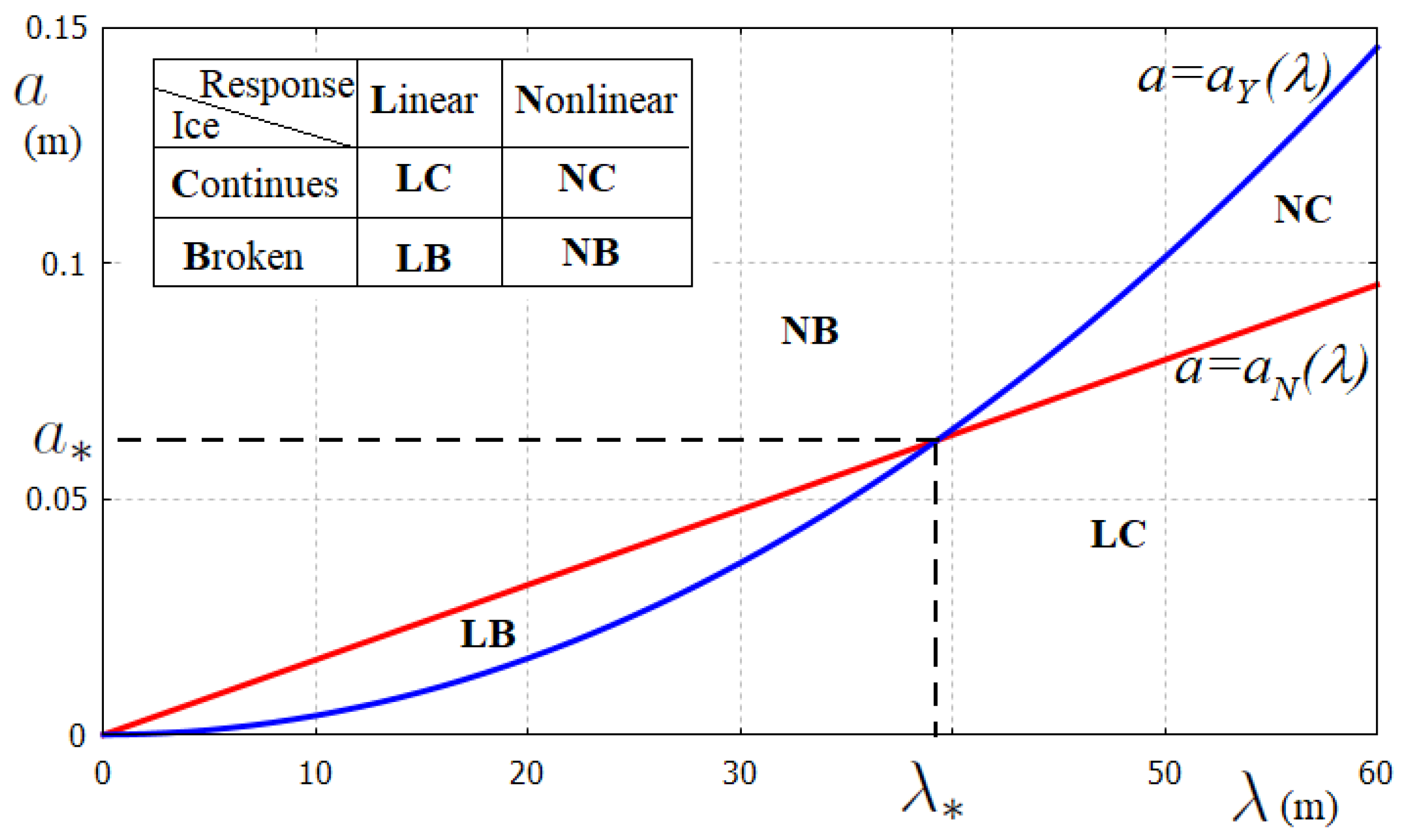
Therefore, sinusoidal waves in a continuous ice of thickness $h_i$ do not exist if the wave amplitude exceeds the right-hand side of (8). The line $a=a_Y\left(\lambda \right)=({\epsilon }_Y/\left(2{\pi }^2{h}_i\right){\lambda }^2$ is shown in Figure 1 by the blue line for ${\epsilon }_Y=8\times {10}^{-5}$ and $h_i=10$ cm. It is seen that the ice sheet can be treated as continuous for wavelength $\lambda =50$ m for a wave amplitude up to 10 cm. The linear model of FGWs can be questionable for such high waves. If the inequality (8) is not satisfied then the ice should be modelled as broken ice.

A flexural-gravity wave can be approximated as a linear one if the product $ak$ is small; see [34,35,36], where second-order FGWs were analysed. The results of the second-order analysis were compared with the experimental results for a plate made of closed-cell rubber sponge in [5]. The plate thickness was 2 cm. All the studied waves were of amplitude 2 cm with wavelengths from 0.92 m to 3.31 m. The product $ak$ varied in the experiments from 0.038 to 0.1366. The theoretical and experimental ratios of the second-order wave amplitude to the linear wave amplitude were shown in Figure 14 of [5] for the mentioned interval of the wavelengths. The comparison confirmed that the nonlinear terms can be neglected with accuracy $O\left(ak\right)$. The maximum ratio 0.14 measured in the experiments occurred at $\lambda =1.24$ m, which was close to the resonant wavelength predicted by the second-order wave theory. Even in this case, with $ak=0.101$, the contribution of the nonlinear effects is of the order of $O\left({\left(ak\right)}^2\right)$. In general, the linear FGW theory can be used if $ak<\delta$, where the value of $\delta$ depends on the wave conditions and required accuracy. As a conservative estimate and a reference case, we take $\delta =0.01$. The line $a=a_N\left(\lambda \right)=\delta /\left(2\pi \right)\times \lambda$ is depicted in Figure 1 in red for $\delta =0.01$. The lines $a=a_N\left(\lambda \right)$ and $a=a_Y\left(\lambda \right)$ intersect at ${\lambda }_{*}=(\pi \delta /{\epsilon }_Y)h_i$, where $a_{*}=({\delta }^2/2{\epsilon }_Y)h_i$. The lines divide the quarter of plane $\lambda >0$ and $a>0$ in four regions (see Figure 1), where LB is for linear waves in broken ice, LC is for linear waves in continuous ice, NB is for nonlinear waves in broken ice and NC is for nonlinear waves in continuous ice. We may conclude that nonlinear FGWs in continuous ice occur, in general, for long waves, $\lambda >{\lambda }_{*}$, of large amplitude with $a_N\left(\lambda \right)<a<a_Y\left(\lambda \right)$.

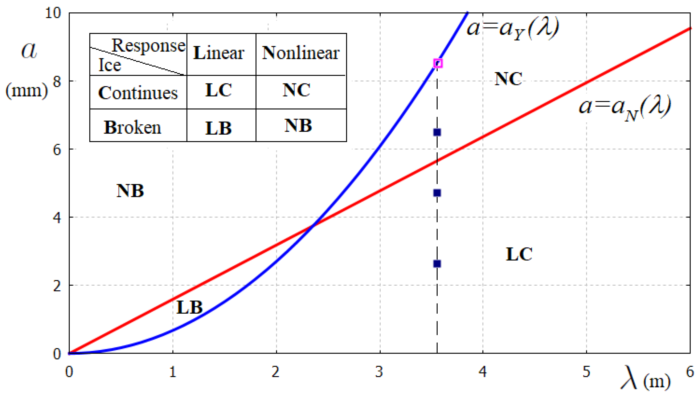
The interaction of water waves with ice was studied experimentally in [37]. The amplitudes of FGWs propagating into an ice plate of 6 mm thickness were found to be approximately two times smaller than the amplitudes of the incident water waves. The effects of current and wind on the FGW amplitudes were also studied. The plane $(\lambda ,a)$ for $h_i=6$ mm and the elastic characteristics of sea ice are shown in Figure 2, where the markers are for the experimental results from [37] without current and wind. The wavelength $\lambda =3.55$ m was obtained using the dispersion relation (6) for the generated wave period 1.5 s. The FGW amplitude $8.5$ mm, at which the ice sheet breaks, was recovered in the experiments (see Figure 5 in [37]), and it is shown by the magenta marker in Figure 2 of our paper. It is seen that the present criterium of ice breaking well corresponds to the experimental finding.

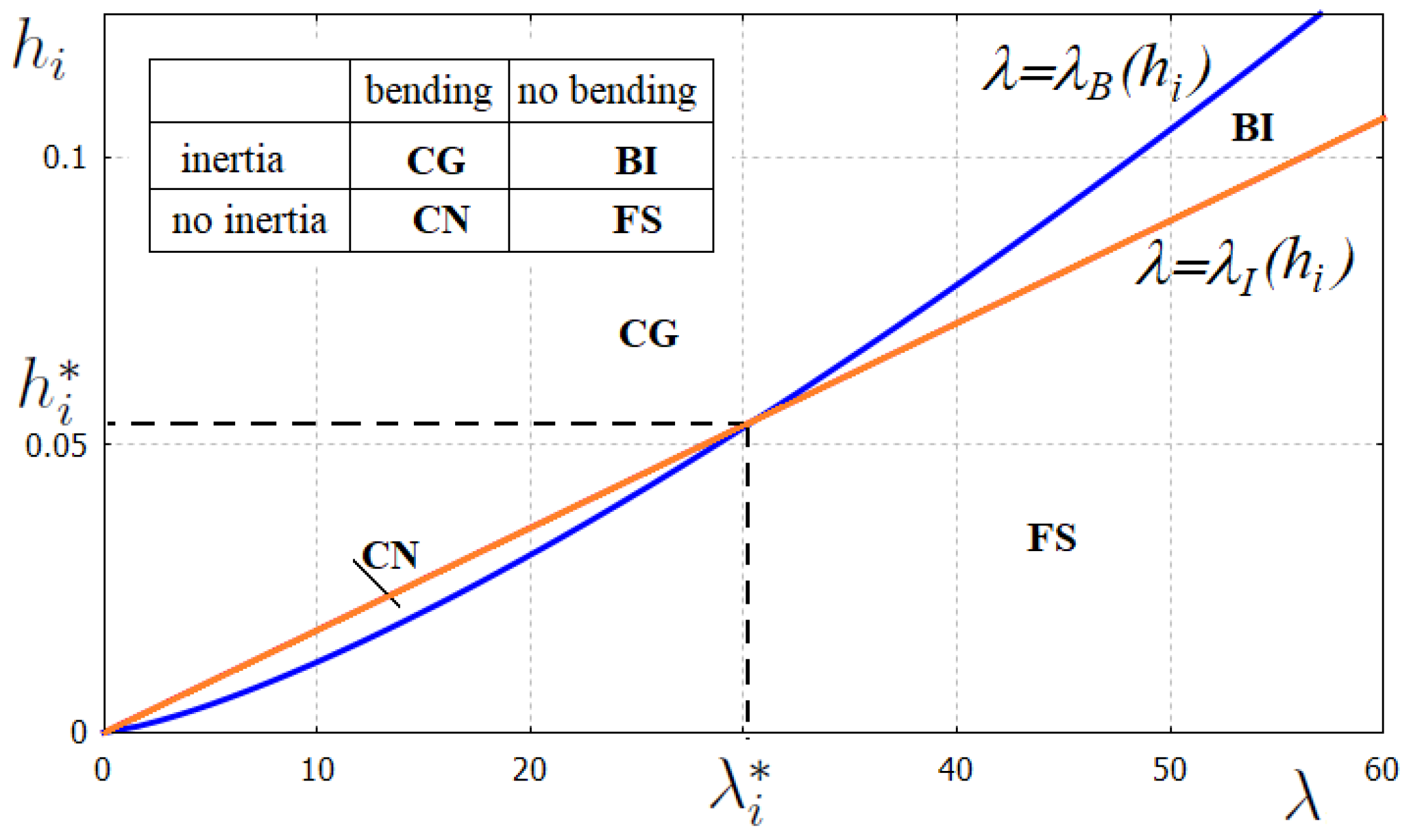
3. Flexural-Gravity Versus Gravity Waves

It is possible that for a long FGW with $\lambda >{\lambda }_{*}$ the bending term $D{k}^4$ in the dispersion relation (6) can be neglected compared to the gravitational term ${\rho }_{w}g$ and the wave can be treated as a gravitational wave but not as an FGW.

The bending term can be neglected if $D{k}^4<{\rho }_{w}g{\delta }_B$, where ${\delta }_B$ is a small dimensionless parameter dependent on the required accuracy. The inequality provides that bending stresses in the ice plate can be neglected for $\lambda >{\lambda }_B\left(h_i\right)$, where

$${\lambda }_B=2\pi h_i^{3/4}{\left[{\displaystyle \frac{E}{12(1-{\nu }^2){\rho }_{w}g{\delta }_B}}\right]}^{1/4}.$$

(9)

For ${\delta }_B=0.01$, which corresponds to the bending term in (6) being less than one percent of the gravitational term and the ice characteristics $E=4.2\times {10}^9$ N/m², $\nu =0.33$, ${\epsilon }_Y=8\times {10}^{-5}$, ${\rho }_w=1026$ kg/m³, $g=9.81$ m/s² from [25], we find that ${\lambda }_B<{\lambda }_{*}$ if

$$h_i>{\displaystyle \frac{4}{3}}{\displaystyle \frac{E}{(1-{\nu }^2){\rho }_{w}g}}{\left({\displaystyle \frac{{\epsilon }_Y}{\delta }}\right)}^4{\displaystyle \frac{1}{{\delta }_B}}={\displaystyle \frac{2.28\times {10}^{-11}}{{\delta }^4{\delta }_B}}m.$$

(10)

The inequality (10) for $\delta ={\delta }_B=0.01$ yields that nonlinear FGWs in ice can be observed only for ice thickness less than 23 cm, where ${\lambda }_B>{\lambda }_{*}$. The wavelengths of these FGWs are in between ${\lambda }_{*}$ and ${\lambda }_B$. The bending effects can be neglected for $\lambda >{\lambda }_B$ and the waves can be approximately treated as gravitational waves. These estimates are valid for linear FGWs, strictly speaking. However, we may accept that the dispersion relation (6) is approximately satisfied even for weakly nonlinear waves; see [38], section 2.1 and discussions there.

The ice inertia that is described by the first term ${\rho }_i{h}_i$ in the brackets on the left-hand side of dispersion relation (6) can be neglected compared with the liquid inertia, which is described by the second term in the brackets, if $2\pi {\rho }_i{h}_i/\left({\rho }_w\lambda \right)<{\delta }_I$, where ${\delta }_I$ is a small dimensionless parameter dependent on the required accuracy. We used, here, $0<tanh\left(kH\right)<1$ for any positive $kH$. Therefore, if $\lambda >{\lambda }_I\left(h_i\right)$, where

$${\lambda }_I={\displaystyle \frac{2\pi }{{\delta }_I}}\left({\displaystyle \frac{{\rho }_i}{{\rho }_w}}\right)h_i,$$

(11)

then the ice inertia can be neglected. The lines $\lambda ={\lambda }_I\left(h_i\right)$ and $\lambda ={\lambda }_B\left(h_i\right)$ are shown on the plane $(\lambda ,h_i)$ for ${\delta }_I=0.01$ and ${\rho }_i=917$ kg/m³; see Figure 3. The other parameters are the same as defined above. Here, ${\lambda }_I=561.57h_i$ and ${\lambda }_B=271.32m^{1/4}{h}_i^{3/4}$. These lines intersect at

$$h_i^{*}={\displaystyle \frac{E}{12(1-{\nu }^2){\rho }_{w}g}}{\left({\displaystyle \frac{{\rho }_w}{{\rho }_i}}\right)}^4{\displaystyle \frac{{\delta }_I^4}{{\delta }_B}}=5.45·{10}^4{\displaystyle \frac{{\delta }_I^4}{{\delta }_B}}m.$$

(12)

For ${\delta }_I={\delta }_B=0.01$, we have $h_i^{*}=5.45$ cm, and the corresponding wavelength is ${\lambda }_i^{*}=30.6$ m.

The lines $\lambda ={\lambda }_I\left(h_i\right)$ and $\lambda ={\lambda }_B\left(h_i\right)$ divide the quarter of plane $\lambda >0$ and $h_i>0$ into four regions, where FS is for gravity waves without account for the ice presence, CN is for continuous ice without ice inertia, BI is for broken ice with inertia and CG is for the most general model of linear FGWs with account for bending and inertia effects. The model of continuous ice without inertia (see region CN in Figure 3), which is popular in theoretical studies (see [39], for example), can be used only for very thin ice and short waves.

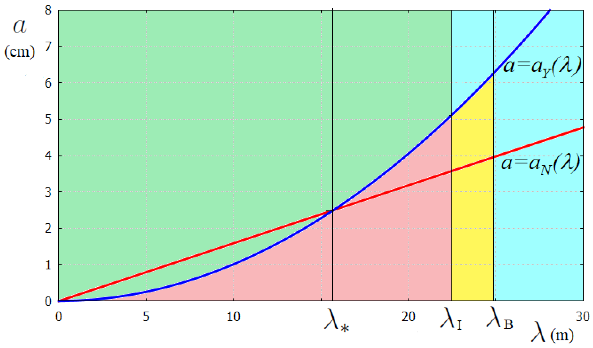
4. Further Simplifications of FGW Descriptions

The classification of FGWs starts with Figure 3. For the given characteristics of the ice and the liquid under the ice, $E,\nu ,{\rho }_i,{\rho }_w,g$, and for the required accuracy parameters, ${\delta }_I,{\delta }_B,\delta$, we plot the curves $\lambda ={\lambda }_I\left(h_i\right)$ and $\lambda ={\lambda }_B\left(h_i\right)$. If the ice thickness $h_i$ is smaller than $h_i^{*}$ then we have three intervals of the wavelength, as follows: $0<\lambda <{\lambda }_I\left(h_i\right)$, where both the bending and inertia of the ice plate matter, ${\lambda }_I\left(h_i\right)<\lambda <{\lambda }_B\left(h_i\right)$, where plate bending matters but plate inertia is minor, and $\lambda >{\lambda }_B\left(h_i\right)$, where both the plate inertia and bending are minor and the presence of the ice plate can be disregarded. We will use, in the following, $\delta ={\delta }_I={\delta }_B=0.01$. Inequality (10) gives that ${\lambda }_B\left(h_i\right)<{\lambda }_{*}$ for $h_i>22.8$ cm. To illustrate the analysis, we take $h_i=4$ cm. Then, ${\lambda }_{*}=15.7$ m, ${\lambda }_I=22.46$ m, ${\lambda }_B=24.87$ m and ${\lambda }_{*}<{\lambda }_I<{\lambda }_B$; see Figure 4 for the corresponding plane $(\lambda ,a)$. Combining the classifications of the FGWs in planes $(h_i,\lambda )$ and $(\lambda ,a)$, we distinguish eleven cases summarised in

Table 1. Eleven cases of FGWs for $h_i<h_i^{*}$.

$0<\lambda <{\lambda }_{*}$	$0<a<a_Y$	linear FGWs
$0<\lambda <{\lambda }_{*}$	$a_Y<a<a_N$	linear waves in broken ice
$0<\lambda <{\lambda }_{*}$	$a>a_N$	nonlinear waves in broken ice
${\lambda }_{*}<\lambda <{\lambda }_I$	$0<a<a_N$	linear FGWs
${\lambda }_{*}<\lambda <{\lambda }_I$	$a_N<a<a_Y$	nonlinear FGWs
${\lambda }_{*}<\lambda <{\lambda }_I$	$a>a_Y$	nonlinear waves in broken ice
${\lambda }_I<\lambda <{\lambda }_B$	$0<a<a_N$	linear FGWs without ice inertia
${\lambda }_I<\lambda <{\lambda }_B$	$a_N<a<a_Y$	nonlinear FGWs without ice inertia
${\lambda }_I<\lambda <{\lambda }_B$	$a>a_Y$	nonlinear gravity waves
$\lambda >{\lambda }_B$	$a<a_N$	linear gravity waves
$\lambda >{\lambda }_B$	$a>a_N$	nonlinear gravity waves

.

The obtained wave classification for $h_i=4$ cm is depicted in Figure 4, where the green region is for waves in broken ice, the red region is for FGWs, the yellow region is for FGW without inertia and the light blue region is for gravity waves. The nonlinear waves correspond to the part of the $(\lambda ,a)$-plane above the red straight line $a=a_N\left(\lambda \right)$ and the linear waves to the part below that line.

The water under the ice can be considered as shallow when $tanh\left(kH\right)$ in (6) can be approximated as $kH$ with a given relative accuracy ${\delta }_S$. Correspondingly, the water can be approximated as infinitely deep if $tanh\left(kH\right)\approx 1$ with a given accuracy ${\delta }_{\infty }.$ Selecting ${\delta }_{\infty }={\delta }_s=0.01$ and using the estimates

$${\displaystyle \frac{tanhx-x}{x}}<0.01\mathrm{for}x<0.174$$

and

$${\displaystyle \frac{1-tanhx}{1}}<0.01\mathrm{for}x>2.7$$

we conclude that the shallow water approximation can be used for $H<0.027\lambda$ and deep water approximation can be used for $H>0.43\lambda$ with a relative error less than 1%. As a reference case, see Figure 4; for $\lambda =20$ m, the water is shallow if $H<54$ cm and infinite deep if $H>8.6$ m. If the water depth is greater than $\lambda /2$, roughly, then the actual bottom topography does not matter, which is important in problems with complex bottom topography.

Dispersion relation (6) is approximated by a sixth-order polynomial equation for shallow water and by a fifth-order polynomial equation for deep water. The polynomial equations are easier to solve than the original transcendental Equation (6). The roots of Equation (6) have been analysed in [40], Section 6. It is shown in [41], Section 5, that some roots of (6) can be double or even triple roots. Helpful estimates of the roots were obtained in [42], Section 4. The authors are not familiar with comprehensive classification of roots of dispersion Equation (6) for different parameters of the problem.

Concerning the linear plate Equation (1), the ice can be modelled as a thin plate if $h_i<\lambda /10$ or thinner, and the ice response is linear if the gradient of the ice deflection, $\partial w/\partial x$, is small. The nonlinear terms in the more general nonlinear equations of a thin elastic plate (see [39]), which are of the order of ${\left(w_x\right)}^2$, can be neglected with relative accuracy of 1% if $a<\lambda /\left(20\pi \right)$. We conclude that Equation (1) can be used for analysis of FGW if $h_i<\lambda /10$ and if the wave amplitude $a<\lambda /\left(20\pi \right)$. Adding the line $a=\lambda /\left(20\pi \right)$ to Figure 1, we can observe that nonlinearity of FGWs is caused mainly by nonlinear hydrodynamics (see Equations (2) and (4)), but not by nonlinearity of the ice deflection. Adding the line $h_i=\lambda /10$ to Figure 2, we may conclude that the wave classification presented here corresponds to thin elastic plate approximation. The ice sheet should be modelled as a plate of a finite thickness only for very short waves.

5. Conclusions

In the study of the particular problem of floating ice response, it is safe to employ a most general model of ice and its interaction with the underlying water. In such a model, ice porosity and anisotropy, viscosity, finite nonconstant thickness and many other effects are included. The numerical results predicted by the model can be difficult to explain. It can also be difficult to separate physical effects from effects induced by the numerical algorithm. In this way, computations provide data files similar to files with laboratory or field measurements, which require their own thorough analysis. The analysis of the data means that we should identify the most important factors (as a rule of thumb, there are two, seldom three, factors governing a studied process) and estimate the contributions of other effects, which modify the main result but do not change its meaning.

The study performed in this paper gives ideas on how such an analysis can be performed. Even though we limited ourselves to linear FGWs, the presented analysis can be used for many other problems. For example, if we study a surface-effect ship moving on sea ice, we can estimate the magnitude of the ice deflection from the static configuration and the length scale $\lambda$ of the ice response, using the known speed of the vessel and the dispersion relation (6). The measured water depth, which is necessarily constant, and the estimated length scale $\lambda$ give us ideas about possibility, so as to approximate water as shallow or of infinite depth. The length scale and measured/estimated ice thickness can either support a thin plate model of ice or guide us towards a more complicated model of ice cover. Estimates of nonlinear, bending and inertia effects, as they are explained in this paper, lead to further/deeper analysis of the studied process. Potentially, after this analysis and these simplifications, we can arrive at a reasonable parsimonious model, predictions of which are not very different from the results of computations within the most complete model.

In the calculations of this paper, the relative accuracies $\delta$, ${\delta }_I$, ${\delta }_B$, ${\delta }_{\infty }$, ${\delta }_S$ were taken as 1%. Changes of the accuracies, either for particular purposes or particular studies, will change the boundaries of the regions in Figure 1, Figure 2 and Figure 4 for some environmental conditions. In particular, the yellow region in Figure 4 for FGWs without ice inertia can be significantly enlarged when ${\delta }_I$ is increased. The calculations were performed for particular values of yield strain, Young modulus, Poisson’s ratio and densities of the ice and water. Variations of these characteristics will shift the boundaries in Figure 4. Other possible criteria of ice failure will also move the boundaries. However, the relative positions of the regions in Figure 4 are expected to be independent of all these variations.

The preliminary results of this study were presented at the workshop “Mathematics of sea-ice”, 22–23 January 2024, Norwich, UK and at the International Innovation & Cooperation in Naval Architecture and Marine Engineering Conference, 22–25 August 2024, Harbin, China.