Experimental Investigation on IceBreaking Resistance and Ice Load Distribution for Comparison of Icebreaker Bows

Abstract

During icebreaker navigation in ice-covered waters, icebreaking resistance and dynamic ice loads acting on the bow critically determine the vessel’s icebreaking performance. Quantitative characterization of the icebreaking resistance behavior and ice load distribution on the bow is essential for elucidating ship-ice interaction mechanisms, assessing icebreaking capability, and optimizing structural design. This study conducted comparative icebreaking tests on two icebreaker bow models with distinct geometries in the small ice model basin of China Ship Scientific Research Center (CSSRC SIMB). Systematic measurements were performed to quantify icebreaking resistance, capture spatiotemporal ice load distributions, and document ice failure patterns under level ice conditions. The analysis reveals that bow geometry profoundly influences icebreaking efficiency: the stem angle governs the proportion of bending failure during vertical ice penetration, while the flare angle modulates circumferential failure modes along the hull-ice interface. Notably, the sunken keel configuration enhances ice clearance by mechanically expelling fractured ice blocks. Ice load distributions exhibit pronounced nonlinearity, with localized pressure concentrations and stochastic load center migration driven by ice fracture dynamics. Furthermore, icebreaking patterns—such as fractured ice dimensions and kinematic behavior during ship-ice interaction—are quantitatively correlated with the bow designs. These experimentally validated findings provide critical insights into ice-structure interaction physics, offering an empirical foundation for performance prediction and bow-form optimization in the preliminary design of icebreakers.

1. Introduction

Icebreaking is a highly complex process, which, depending on the interaction mode between ice and vessel, can be characterized as a cyclic sequence of breaking, rotation, immersion, and sliding of ice along the hull [1]. The icebreaking performance serves as a critical metric for assessing the operability of icebreaking vessels, playing a pivotal role in preliminary design and optimization by informing the selection of installed power and propulsion systems, thereby achieving the desired icebreaking capability and operational efficiency. The bow form significantly influences ice failure modes and icebreaking effectiveness. As early as 1889, Runeberg [2] noted that reducing the stem angle helps decrease resistance, while Makinen (1973) [3] quantified that ice resistance can be reduced by approximately 60% when the stem angle decreases from 82° to 20°. Subsequent studies by Su et al. (2010), Sawamura (2012), and Valanto (2001) [4,5,6] employed various methodologies to investigate the effect of bow geometry on the icebreaking process. Shodi (1995) [7] proposed that in icebreaker bow design, an increasing flare angle combined with decreasing waterline and stem angles tends to improve performance. Currently, analyses of bow geometry mainly focus on icebreaker bows characterized by small stem angles and large flare angles. Enkvist (1972) and Lindqvist (1989) [8,9] developed empirical formulas tailored for such configurations. Utilizing HSVA (Hamburgische Schiffbau- Versuchsanstalt GmbH) ice tank test data collected between 1996 and 2014, Myland et al. (2016) [10] quantified the influence of various bow geometries on icebreaking resistance and failure modes. More recently, Hisette et al. (2019) [11] evaluated the impact of bow parameters—including stem and waterline angles—on the icebreaking process of conventional ship bows, finding that ice bending and fracturing intensified as the waterline angle decreased, accompanied by an increase in ice immersion.

Current ice resistance prediction techniques primarily encompass model testing, numerical simulations, and empirical formulations. Among these, model tests conducted in ice tanks remain the most accurate method for replicating actual ice conditions and ship-ice interaction scenarios, allowing precise control of testing parameters and providing profound insight into underlying physical relationships. For conventional wedge-shaped icebreaker bows with small stem and waterline angles, bending failure generally predominates as the principal ice failure mode. However, Kamarainen (1993) [12] identified extrusion failure occurring at the shoulder region during testing, demonstrating that the bow also imposes extrusion and shear stresses on the ice sheet. Wang and Jones (2008) [13] conducted icebreaking resistance tests on the Canadian Coast Guard ship Terry Fox model under level ice conditions and validated the applicability of ice tank results by comparison with full-scale trial data. Von Bock (2010) [14] performed a series of icebreaker model tests to investigate the influence of hull motions, specifically pitch and heave, on mean and extreme ice resistance values. Extending research beyond traditional icebreaking bows, Müller (2018) [15] tested five bow types, comprising two with bulbous bows and three with large stem angles, under varying ice thicknesses and speeds. Myland et al. (2021) [16] examined ice failure modes, ice resistance, and resistance components for the non-icebreaking DTMB5415 hull form during the icebreaking process, subsequently developing an ice resistance prediction methodology. Sun (2023) [17] conducted a non-icebreaking bow under different levels of ice thicknesses and speeds. During the tests, the total resistance of the model ship was measured, accompanied by the monitoring of the ice load at the stem area with a flexible tactile sensor sheet. Compared with the test results of icebreaker models in former studies, the total ice resistance, as well as the stem ice load, of the present ship was significantly higher.

During icebreaker and sea ice interaction, structural-ice loads exhibit pronounced spatiotemporal nonlinearity. The location and magnitude of high-pressure zones vary dynamically, complicating forecasting efforts. Spatial nonlinearity manifests as uneven distribution of ice loads, with localized high-pressure regions capable of inducing large load peaks, potentially leading to structural damage or safety hazards. Jordaan (1987) [18] analyzed the extrusion interaction between ice sheets and flat surfaces, concluding that ice load distribution concentrates within high-pressure zones, which evolve concurrently with ice failure. Varsta (1983) [19] employed mathematical modeling to investigate ice loads on the hull-ice interface, deriving formulas for average ice pressure while considering hull stiffness and failure progression. Numerical simulations by Su (2011) and Tian (2013) [4,20] quantified ice load magnitudes and vessel response motions. Zhou et al. (2013) [21] utilized model tests to examine the spatial distribution and temporal shifts of ice loads on hulls at varying heading angles. Mikko Kotilainen et al. obtained data on sea ice thickness and icebreaker ship speed in the Baltic Sea and identified ice loads from the measurement data using a Rayleigh separator. Assuming that the ice loads are generated by a common stochastic process, they studied the relationship between the ship speed, ice thickness, and ice loads [22]. Due to the extensive randomness in ice conditions, ice behavior, and contact scenarios, ice loads measured on the hull frames always show high stochastics. Typically, the load peaks are of concern [23].

In this study, two icebreaking bow forms with distinct stem and flare angles were selected for comprehensive ice tank model testing. The ice failure modes, characteristics, and motions of broken ice in front of the bow were observed in detail. The influence of bow geometry on icebreaking resistance was analyzed, alongside investigations into the spatial distribution and temporal evolution of ice loads acting on the bow.

2. Ice Model Basin and Model Ice in CSSRC

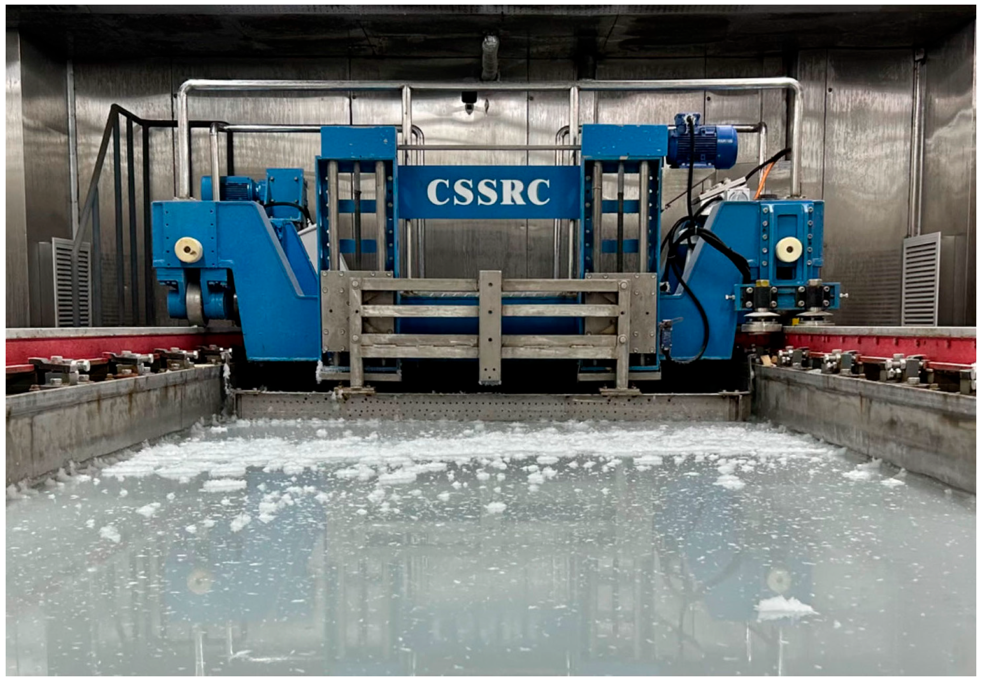
The experiments were performed in the Small Ice Model Basin at China Ship Scientific Research Center (CSSRC, SIMB, Wuxi, China). The basin is 8 m long, 2 m wide, and has a depth of 1 m (Figure 1). The model ice used in the tests was naturally grown columnar-grained model ice frozen from a sodium chloride solution. The seeding method was used to create the initial ice layer. The freezing temperature was kept at −20 °C. After reaching the target thickness, the strength was adjusted by raising the air temperature and warming the ice sheet. When the target strength was reached, the air temperature was kept constant, and the test was started (Tian, 2020) [24].

Through a series of mechanical properties measurements [25], the ice density of the model is 900~920 kg.m⁻³, the initial flexure strength is 60~120 kPa, the initial compressive strength is 150~250 kPa, the initial elastic modulus is 80~200 MPa, and the ratio of the elastic modulus to the bending strength is 1500~2000. In line with the recommendations put forward by Timco (1979) [26], the ratio of elastic modulus to bending strength is about 2000, and the ratio of bending strength to compressive strength is 2.5–3.0.

Table 1. Main physical and mechanical properties of model ice.

Parament	Unit	Value
Density	kg·m−3	900~920
Thickness	mm	10~100
Flexure Strength	kPa	60~120
Compressive Strength	kPa	150~250
Elastic Modulus	MPa	120~200
Elastic Modulus/Flexure Strength	/	1500~2000
Compressive Strength/Flexure Strength	/	2.5~3.0

lists the range of main characteristic parameters of ice in the CSSRC SIMB model.

3. Test Model and Test Method

To research the effects of ship form parameters on ship-ice interaction, ice failure mode, ice resistance, and load generation and evolution, a series of ice tank model tests were carried out with two typical icebreaker bow models with different form parameters, and the ice-bow interaction process, ice resistance, and surface load distribution were monitored.

3.1. Scaling Relationship

The scaling relationship plays an important role in the model test and is the theoretical basis to guide the test. The Froude scaling criterion and Cauthy scaling criterion should be followed in the experiment of ship-ice interaction, which has both a fluid test and a material test.

The Froude scaling criterion is as follows:

$$F\mathrm{r}={\displaystyle \frac{V}{\sqrt{gL}}}$$

(1)

The Cauthy scaling criterion is as follows:

$$C\mathrm{a}={\displaystyle \frac{V}{\sqrt{E/\rho }}}$$

(2)

When the test meets both types of scaling criteria, the reduction ratio of the model geometric length, ice strength, thickness, and elastic modulus is λ, the model scale of time and speed is λ^1/2, and the model scale of mass and force is λ³.

The purpose of this experiment is to investigate the bow-ice interaction performance and to observe the icebreaking resistance and failure modes. Accordingly, a scale ratio of 1:30 was adopted.

3.2. Test Model

The forms of bow selected in this series are low-ice polar class icebreakers (Bow A, PC6), and medium-ice polar class icebreakers (Bow B, PC3). The two forms of ships both adopt the design of a small stem angle and a large flare angle. The main dimensional parameters of the model are shown in

Table 2. Main ship form parameters.

Parament	Bow A	Bow B
Length (m)	1.01	1.32
Width (m)	0.62	0.63
Depth (m)	0.33	0.35
Draught (m)	0.23	0.23
Stem Angle (°)	24	20
Water Angle (°)	54	80
Flare Angle (°)	53	57

. Among them, Bow B adopts the sunken keel, which is conducive to ice breaking, resistance reduction, and broken ice discharge.

The bow forms are shown in Figure 2.

3.3. Test Method

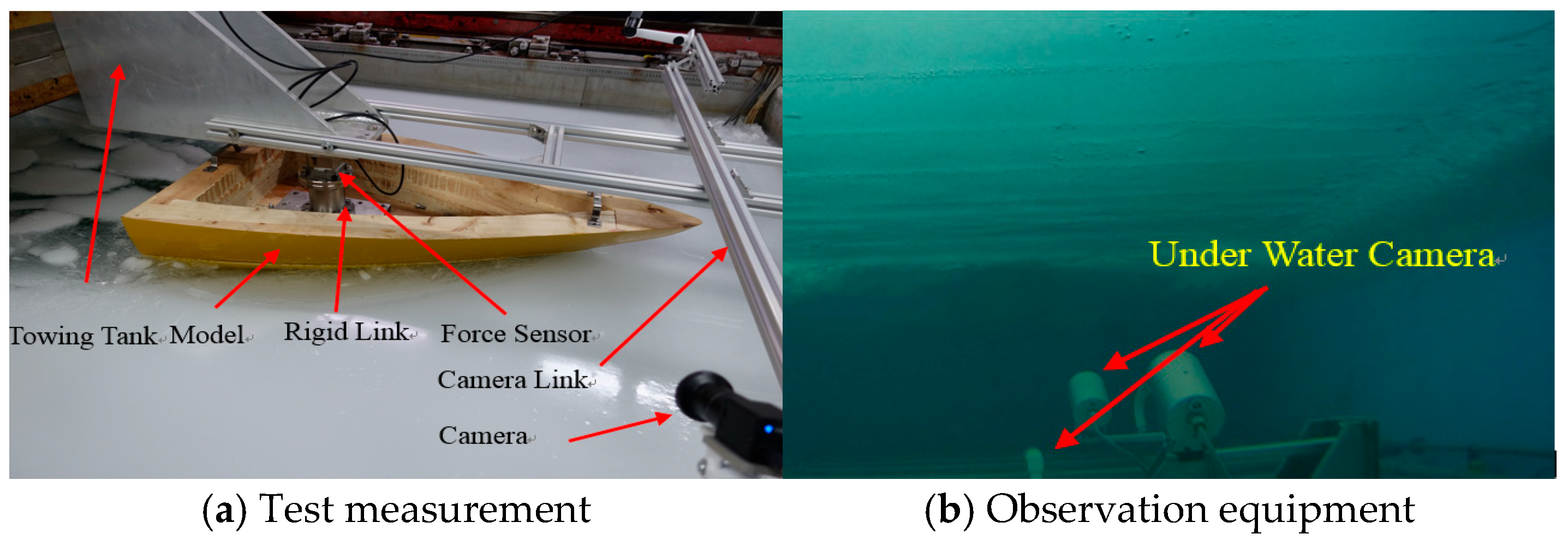
The experimental protocol employed static towing of the ship model through ice sheets to investigate bow resistance characteristics and ice failure mechanisms during polar navigation. The bow model was rigidly coupled to the test carriage via a uniaxial load cell, with the sensor’s mounting interface precisely aligned at the bow’s geometric centroid and orthogonal to the waterplane. A tri-camera imaging system, comprising three industrial-grade units positioned at the bow and port/starboard quarters, synchronously documented ice-structure interaction dynamics and fracture propagation patterns. Complementary underwater videography utilized three fixed submersible cameras strategically deployed beneath the ice sheet to capture fracture kinematics and fragment transport phenomena (Figure 3).

In order to study the spatiotemporal evolution of the ice load on the bow and the similarities and differences of the ice load of different ship forms. A distributed tactile sensor was pasted near the starboard ice line of bow A and bow B (Figure 4). It can record and output the bow-ice load and the slipping evolution of the load in real time.

To study the icebreaking modes, icebreaking resistance, and space-time evolution of the ice load on different bow forms The icebreaking resistance and the space-time evolution distribution characteristics of the ice load of the bow A and bow B were measured at different icebreaking velocities. The selected test velocities were 0.089 m/s, 0.188 m/s, and 0.282 m/s, corresponding to speeds of 1 kn, 2 kn, and 3 kn in full scale, respectively.

4. Test Results and Analysis

In this series of experiments, the typical velocities of icebreakers sailing in the ice region were selected, and the process of ship-ice interaction, icebreaking mode, icebreaking shape, and space-time evolution law of ice load were studied.

4.1. IceBreaking Mode

Video observations of the icebreaking processes for bow A and B bows revealed congruent failure sequences across the three configurations, characterized by three mechanistically linked phases. Initial bow-ice contact-induced localized compressive fracture nucleation at the bow centerline, generating radial crack propagation followed by circumferential fissure development. Subsequent bow advancement caused median cleavage of the ice sheet into port and starboard cantilevered wedges, which underwent progressive flexural failure evidenced by longitudinal cracking along their neutral axes. Post-fracture ice fragment transport exhibited bimodal trajectories: submerged debris migrated aft along the hull’s molded surfaces, while surface floes experienced lateral displacement into the channel periphery through ice-hull frictional coupling, as systematically documented in Figure 5.

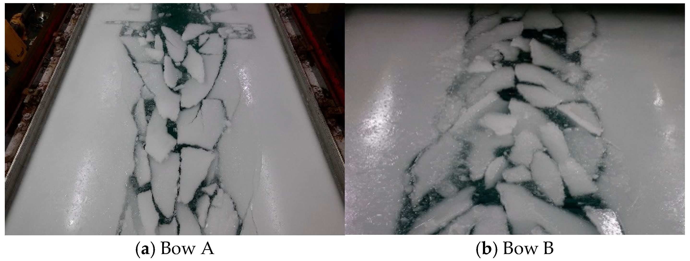
The failure mode of the side ice was also affected by the bow’s form parameters. The research on the bow A and bow B side icebreaking mode was emphasized. In both bows A and B, bending failure is the main failure mode, and the ice sheet has obvious cyclic cracks (Figure 6). Bow B, characterized by a larger flare angle, produced smaller ice fragments along the side hull and exhibited secondary circumferential cracks, whereas such secondary cracking was absent in bow A.

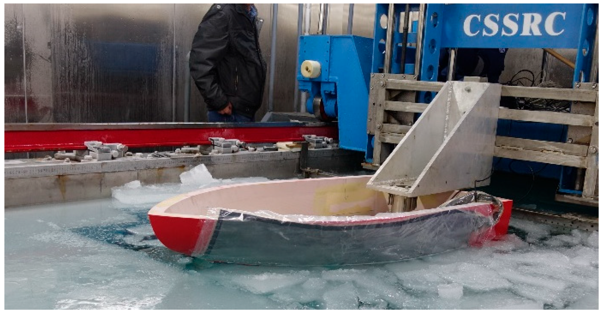
Following the completion of the icebreaking process, the bow model was incrementally retracted to comprehensively document post-fracture ice morphology, including fragment dimensions and spatial distribution patterns (Figure 7). Both A and B bows exhibited analogous ice failure characteristics within the stem-shoulder transitional zone. Circumferential cracks initiated at the stem apex and propagated axially toward the shoulder region, with resultant ice fragments distributed symmetrically along both sides of the channel’s midline. Comparative analysis revealed a direct correlation between bow waterline angles and ice fragment geometry: increased waterline angles enhanced ice fragment regularity while maintaining consistent fracture patterns (Figure 7).

The icebreaking performance of bow A and bow B was investigated through controlled model tests. Bow A featured a stem inclination angle of 24°, while bow B exhibited a reduced stem angle of 20°, emphasizing its compact bow geometry. Comparative analysis revealed that bow B demonstrated more pronounced ice flexural failure modes compared to bow A’s dominance of compressive/shear failure mechanisms. Specifically, bow B displayed fewer crushing and interlocking ice fragments due to its optimized stem geometry (Figure 8).

4.2. Size of Broken Ice and Broken Ice Channel

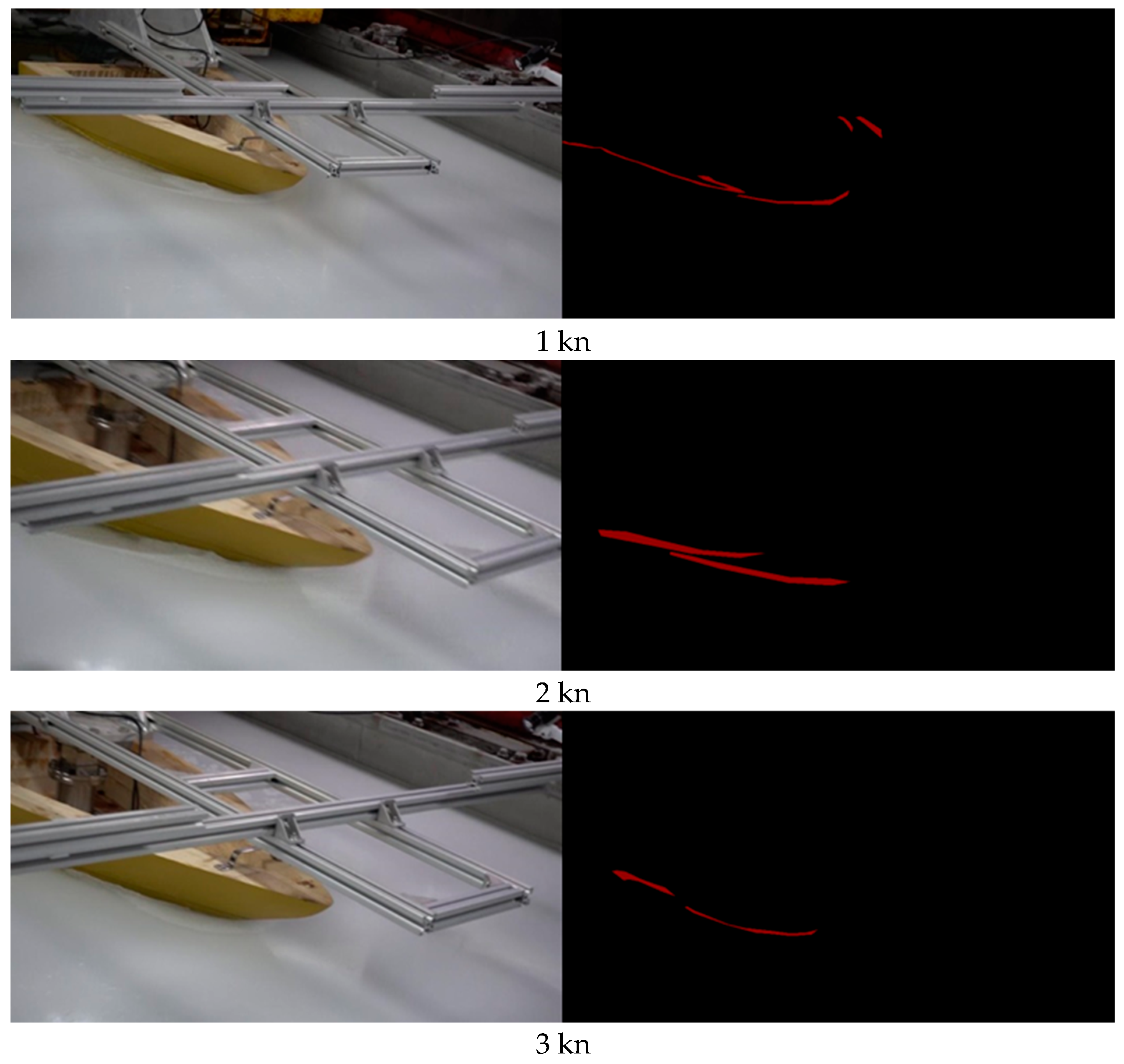
In the context of challenges associated with ice fragmentation characterization and statistical analysis of ice floe dimensions in ice channels under various operational scenarios, this study implemented a DeepLab V3+ deep convolutional image segmentation framework based on TensorFlow to achieve precise segmentation of ice from other media. The methodology enabled the systematic extraction of critical sea ice parameters, including crack propagation patterns, geometric contours, and dimensional characteristics. Comparative analyses were conducted on ice failure crack lengths and ice floe size distributions in broken ice channels under different icebreaking speeds.

Through advanced image recognition techniques, the ice fracture networks surrounding the hull were quantitatively characterized, with particular emphasis on crack length quantification. Statistical results revealed average crack lengths of 0.87 m, 0.52 m, and 0.31 m corresponding to icebreaking speeds of 1 kn, 2 kn, and 3 kn, respectively (Figure 9). The analysis demonstrates an inverse correlation between icebreaking speed and both crack propagation dimensions and fracture network density. Specifically, increased icebreaking velocities were observed to induce reductions in both the characteristic scale of ice failure cracks and the population density of fractures within the damaged ice matrix.

This investigation provides quantitative evidence that larger icebreaking speeds result in more localized fracture patterns with diminished crack lengths and reduced multiplicity, offering valuable insights for optimizing polar vessel operations in ice-infested waters.

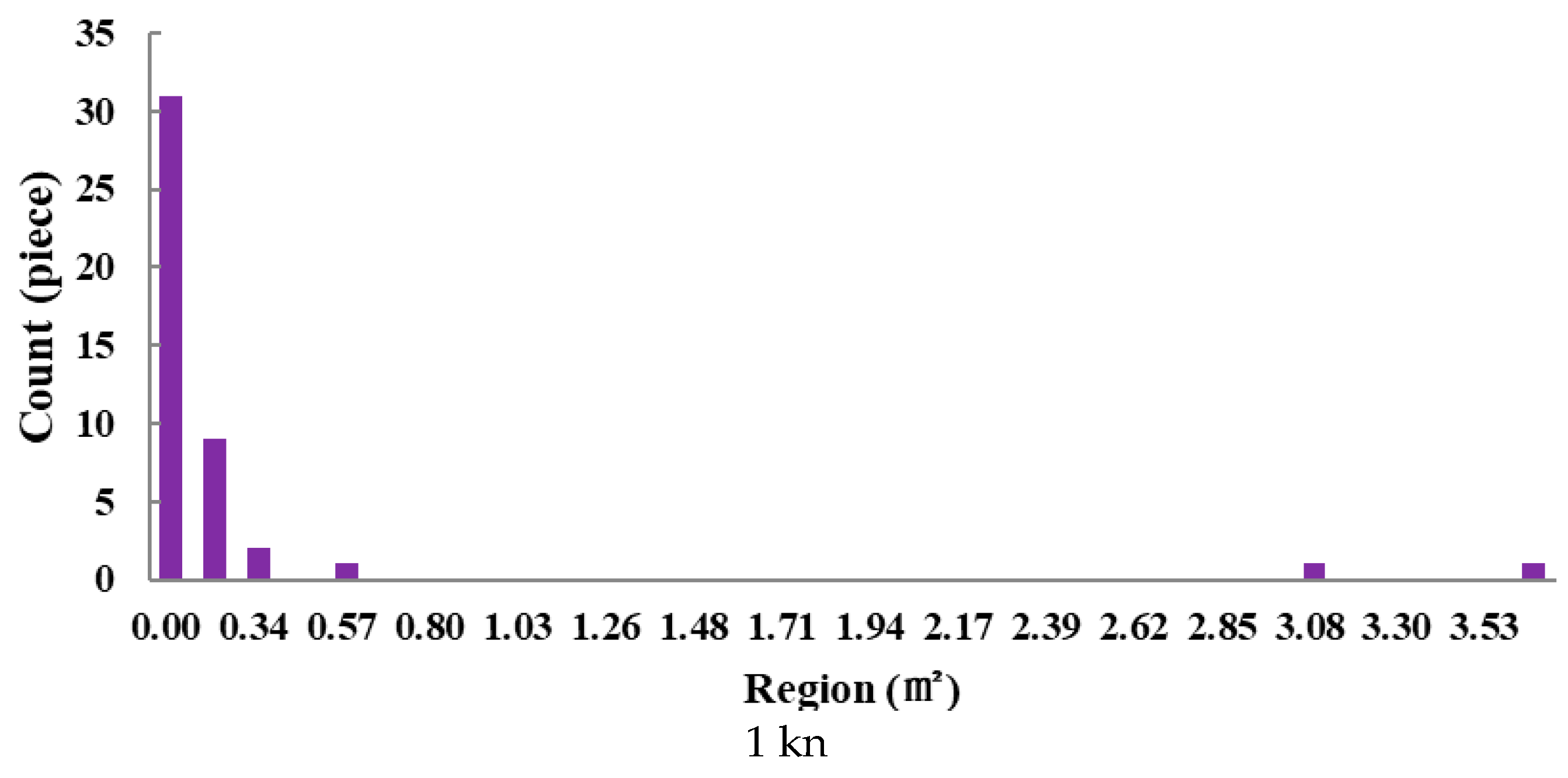
Statistical analysis revealed that smaller ice floes dominate the size distribution within the broken ice channels. At an icebreaking speed of 1 kn, ice floes with areas of 0–0.34 m² accounted for 88.89% of the total population. This proportion increased to 91.11% for floes sized 0–0.19 m² at 2 kn and reached 86.49% for the 0–0.14 m² range at 3 kn (Figure 10). Concurrently, the characteristic size of ice floes exhibited a progressive reduction with increasing icebreaking speeds. Specifically, the dominant size ranges shifted to 0–0.19 m² (1 kn), 0–0.13 m² (2 kn), and 0–0.07 m² (3 kn), demonstrating a clear inverse relationship between operational velocity and ice fragment dimensions (Figure 11).

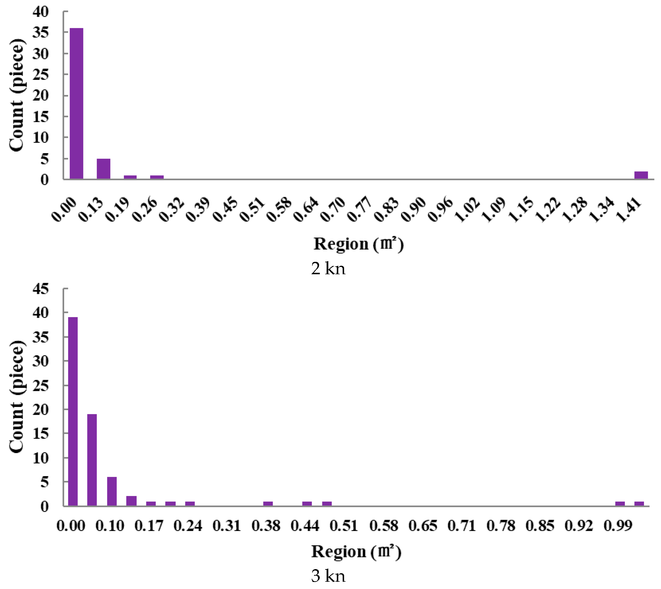
Channel width measurements reveal that at lower icebreaking speeds, the cleared channel exceeds the vessel’s bow width, the size of broken ice at different icebreaking speeds are shown in

Table 3. Size of broken ice at different icebreaking speeds.

Velocity (m/s)	1 kn	2 kn	3 kn
Size (mm)	710	664	635

. As the icebreaking speed increases, the channel width progressively narrows until it converges with the ship’s beam, as illustrated in Figure 12. Video observations from model tests demonstrate that higher icebreaking velocities significantly weaken the compressive action of the bow on adjacent ice layers, thereby reducing the probability of ship-ice collisions and resulting in a narrower channel compared to low-speed operations. Consequently, during icebreaking operations, strategically reducing icebreaking speed—while balancing economic considerations—can widen navigable channels, enhancing safe passage for ice-class transport vessels.

4.3. IceBreaking Resistance

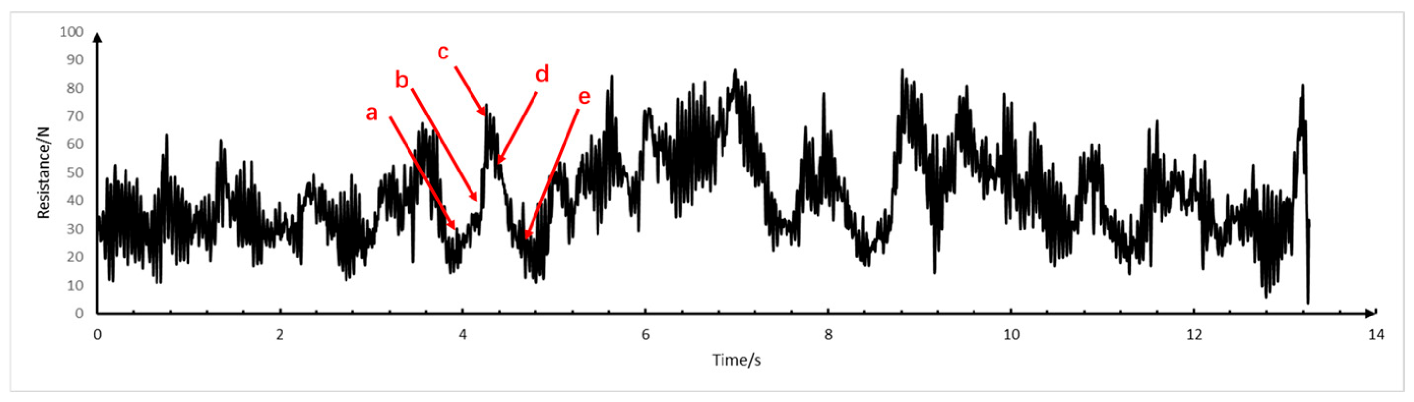
The analysis focused on a discrete icebreaking cycle. During the staged ice-structure interaction process (Figure 13), compressive failure was initiated in the ice sheet upon initial bow contact (Phase a), coinciding with a monotonic rise in ice resistance magnitude. Subsequent flexural failure of the ice sheet (Phase b) marked the attainment of peak periodic resistance, after which fractured ice floes underwent rotational displacement along the hull (Phase c), accompanied by resistance attenuation. During the non-contact interval (Phase d), residual resistance primarily stemmed from sidewall ice friction and kinetic interactions between drifting floes. Cyclicity manifested as renewed bow-ice engagement triggered abrupt resistance escalation (Phase e), restarting the failure sequence. The process exhibited four mechanistic phases: compressive initiation, flexural fracture, rotational transport, and kinetic dissipation, with corresponding time-history ice resistance demonstrating pulsating amplitude modulation synchronized with phase transitions.

By comparing the ice resistance results of bow A and B at different speeds, it can be observed that with the increase in icebreaking speed, the ice resistance generally shows a trend of increasing along with the speed (Figure 14). Comparing the ice resistance values of the two vessels at the same speed, it is found that at lower speeds of 1 to 2 knots, bow B exhibits smaller ice resistance, while at a speed of 3 knots, bow A demonstrates smaller ice resistance.

4.4. Space-Time Evolution of Ice Loads

This experimental series comprehensively investigates the failure mechanisms associated with ship-ice interactions, including structural and sea ice dynamic responses as well as ice fragmentation behavior. Distributed pressure sensors with high sampling rates and spatial resolution were utilized to capture ice-induced loads at structural-ice interfaces, enabling statistical analysis of the distribution of high-pressure zones.

To measure localized ice load distributions on the structure and study icebreaking characteristics, a tactile sensor was employed for partial ice load monitoring during the tests. The tactile sensor had an overall dimension of 1000 mm × 220 mm, with an effective measurement area of 900 mm× 100 mm containing 320 uniformly distributed sensing units, as shown in Figure 15.

The tactile sensor exhibited a measurement range of 1 MPa. Before testing, static calibration was performed using standardized deadweight loading (Figure 16), with verification results confirming measurement errors within 5% of full-scale output, as quantitatively summarized in

Table 4. Tactile sensor calibration data table.

	Temperature (°C)	Weight (kg)	Result (kg)	Error
Tactilus sensor	10	25	24.63	1.47%
		50	52.29	4.57%

.

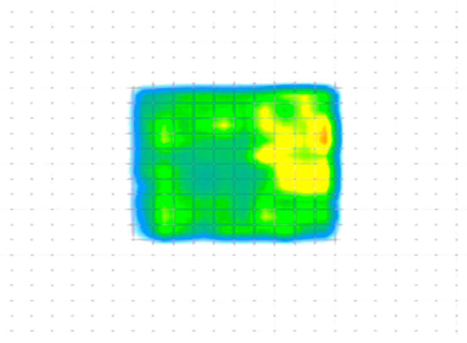
Three-dimensional dynamic mapping of hull-ice loads enables precise observation of load distribution patterns and spatiotemporal evolution of high-pressure zones (HPZs) (Figure 17, the red arrow points to the forward direction of the ship). Initial ice-structure contact occurs at the stem region, generating the primary HPZ during early engagement. As ice failure progresses, the load concentration centroid migrates toward the midship section, forming a secondary HPZ at the shoulder region. Subsequent bow-ice recontact reinitiates compressive loading at the stem, establishing a cyclic load transition sequence. However, quantitative analysis reveals inter-cycle variability in both load magnitude and HPZ spatial coordinates, demonstrating nonlinear spatiotemporal characteristics governed by stochastic ice fracture mechanics.

The total ice load and localized load distributions were mathematically represented using tensor M and its vectorized form M_ijk, where indices i, j, and k denote the row, column, and frame number of the surface load matrix, respectively. The lateral average load and maximum load were calculated through Equations (3) and (4):

$$\overline{H_j}={\displaystyle \frac{1}{n_k}}{\displaystyle {\sum }_{k=1}^{n_k}[\frac{1}{n_i}({\displaystyle {\sum }_{i=1}^{n_i}{M}_{ijk}})]}$$

(3)

$$H_{j,\max }=\underset{1\le k\le n_k}{\max }({\displaystyle \frac{1}{n_i}}{\displaystyle {\sum }_{i=1}^{n_i}{M}_{ijk}})$$

(4)

$\overline{H_j}$, $H_{j,\max }$ represent the mean and maximum ice loads along the i-axis of the load matrix, respectively, the units of them are kPa (Figure 18). Temporal analysis of ice load data during contact events reveals that vertical ice load distributions predominantly concentrate near and below the ice waterline (Figure 19). Notably, high-pressure zones (HPZs) emerge not at the initial contact point but at positions offset downward along the hull’s molded depth, indicating concurrent ice sheet flexural failure and sliding displacement along the draft direction.

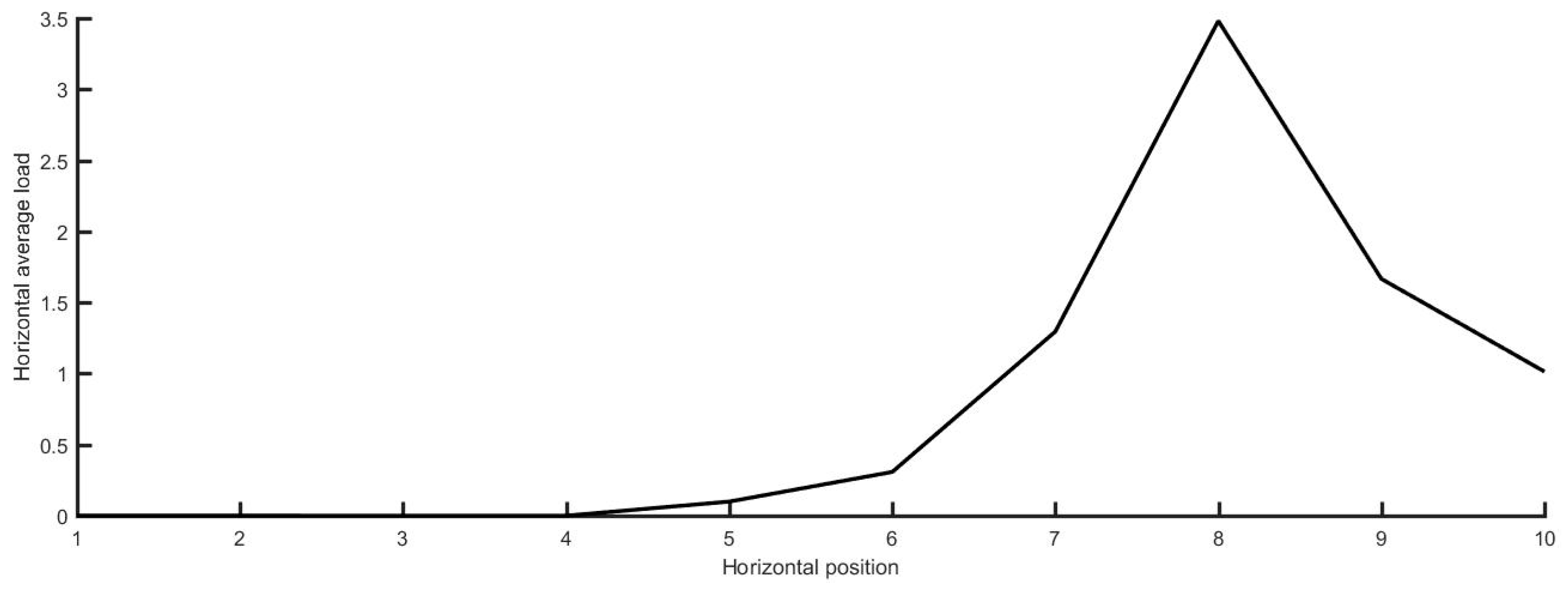
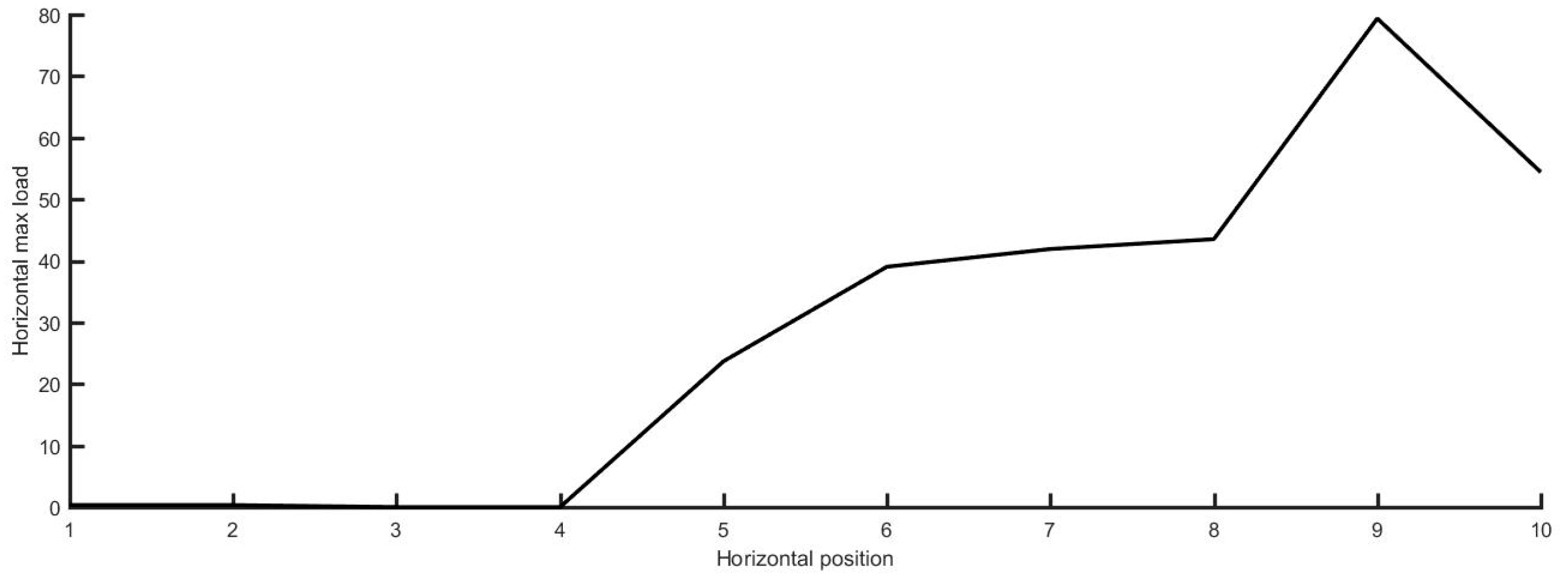
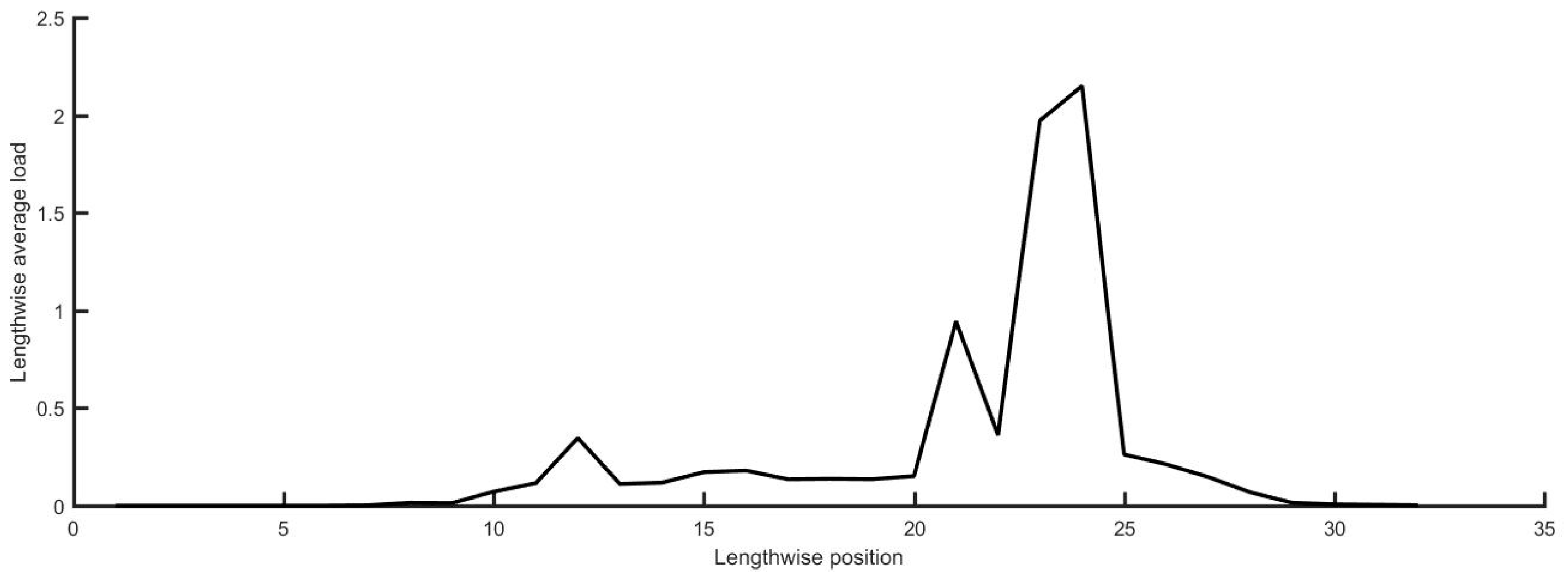
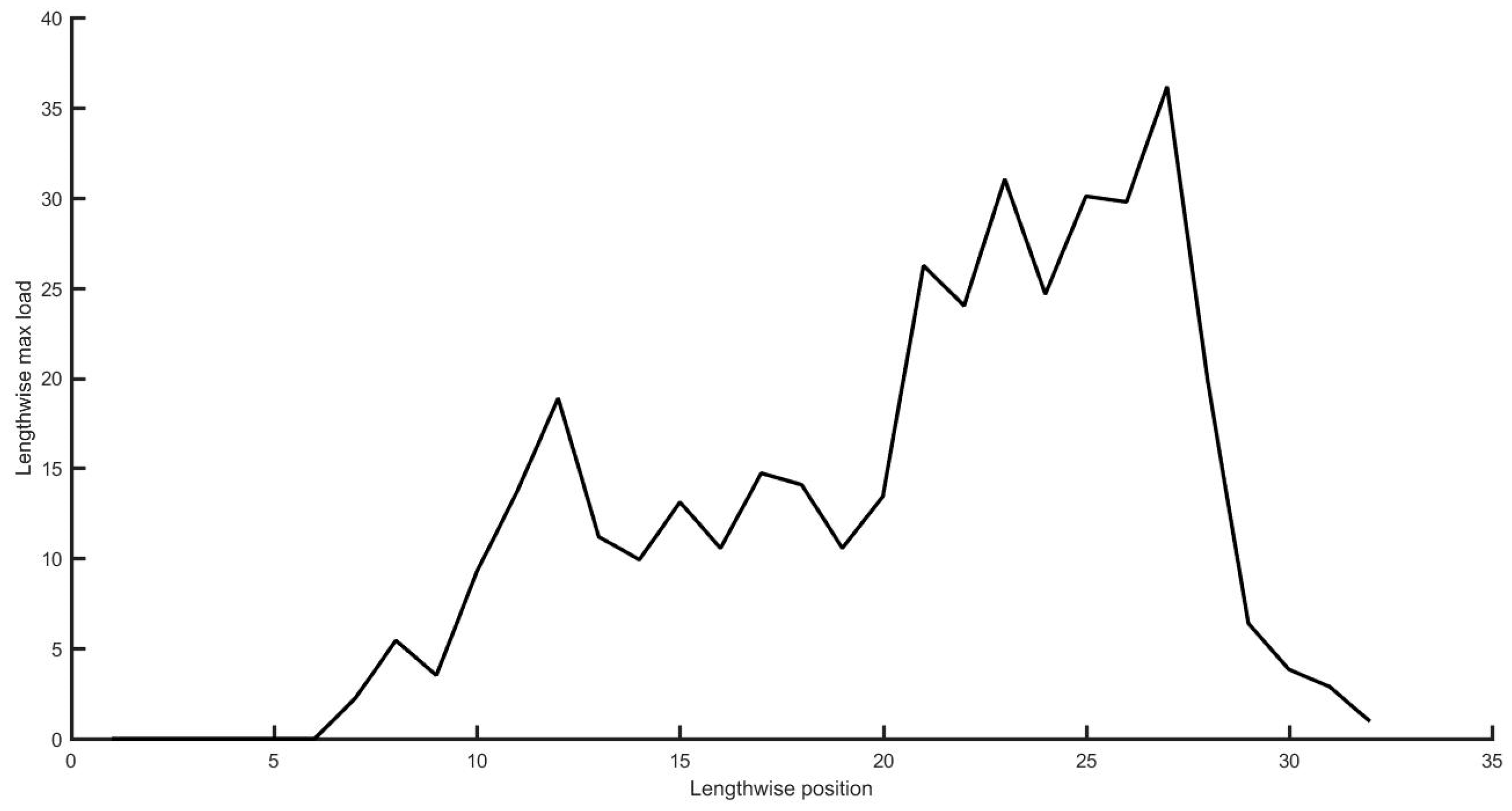
The longitudinal averaged ice load and maximum ice load were calculated using Equations (5) and (6):

$$\overline{V_j}={\displaystyle \frac{1}{n_k}}{\displaystyle {\sum }_{k=1}^{n_k}({\displaystyle {\sum }_{j=1}^{n_j}{M}_{ijk}})}$$

(5)

$$H_{j,\max }=\underset{1\le k\le n_k}{\max }({\displaystyle \frac{1}{n_i}}{\displaystyle {\sum }_{i=1}^{n_i}{M}_{ijk}})$$

(6)

$\overline{V_j}$, $V_{j,\max }$ represent the mean and maximum ice loads along the j-axis of the load matrix, respectively, the units of them are kPa. Simultaneous ice load measurements along the ice waterline revealed two distinct pressure peaks at the bow and shoulder regions, confirming these zones as primary ice-structure interaction areas. Quantitative comparisons showed that both peak and mean ice loads at the bow region exceeded those at the shoulder region, indicating the bow’s dominant role in icebreaking, as illustrated in Figure 20.

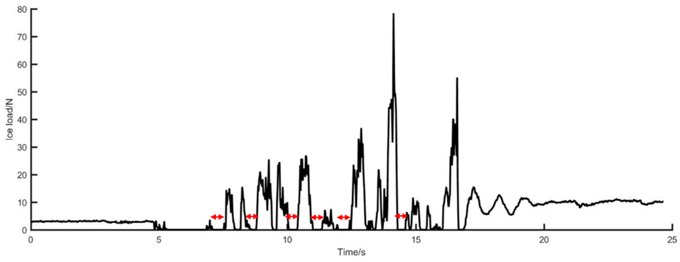
The total ice load acting on the measurement area was calculated using Equation (7):

$$F={\displaystyle {\sum }_{j=1}^{n_j}{\displaystyle {\sum }_{i=1}^{n_i}{M}_{ijk}}}·\mathrm{S}$$

(7)

F is the total ice resistance measured by the tactile sensor, with units in N, while S is the area of the tactile sensor, with units in m².

Time-dependent variation curves of total ice loads in localized regions were generated based on the processed experimental data (Figure 21). The analysis of these curves reveals that load variation patterns in localized regions exhibit congruent trends with the global load dynamics, both demonstrating distinct periodicity and pulsating characteristics. Periodically distributed unloaded intervals observed in the curves further confirm the non-continuous nature of ice-structure contact, indicating intermittent engagement synchronized with icebreaking cycles.

5. Discussion

This study investigated the ice failure modes, resistance characteristics, and spatiotemporal ice load distributions of two bow configurations during polar icebreaking operations. The results indicate that polar icebreakers with reduced stem inclination angles and integrated submerged keels exhibit improvements in resistance performance. Analysis of high-pressure zone (HPZ) migration and contact region slippage during icebreaking cycles highlights the importance of optimizing bow geometry and structural reinforcement in critical areas.

Notably, the fixed towing configuration employed in these model tests imposed full kinematic constraints on hull motions, potentially introducing systemic biases in both resistance measurements and ice load spatial distributions. In future studies, full-scale models will be employed to perform semi-restrained towing and free-sailing tests within larger-scale ice tanks. The resistance and load characteristics will be examined under varying degrees of freedom, while also accounting for the propulsive performance of the propeller. Furthermore, uncertainties encountered during the testing process will be systematically identified and addressed to enhance the reliability and accuracy of resistance and load measurements. This multi-configuration approach aims to establish generalized ice load prediction models accounting for six-degree-of-freedom vessel motions under realistic polar navigation scenarios. For conventional icebreakers, icebreaking capability constitutes the primary design criterion in naval architecture. Additionally, particular attention will be directed toward characterizing the spatiotemporal evolution of critical ice load components such as impact ice loads, localized ice pressures, lateral compressive forces, collisions with floating ice floes, and secondary ice-structure interactions induced by reflection dynamics.

6. Conclusions

This study systematically investigated the ice failure modes, ice fragment dimensions, icebreaking resistance, and spatiotemporal ice load distributions of bow A and bow B bow configurations with distinct icebreaking grades during polar operations. The effects of bow geometry on icebreaking resistance were analyzed, with a particular focus on the temporal-spatial evolution of ice load distributions and ice failure kinematics. The following conclusions were drawn:

(1)

Both bow configurations predominantly induced flexural failure during icebreaking. The bow A exhibited a stem inclination angle of 24°, while the bow B featured a reduced stem inclination angle of 20°. Comparative observations revealed more pronounced flexural failure phenomena and lower proportions of compressive/shear failure modes in the B bow.

(2)

The spatiotemporal evolution of ice loads corresponded with ice-structure contact failure processes. High-pressure zones (HPZs) demonstrated periodic migration from the bow to shoulder regions and back, exhibiting both stochastic and nonlinear characteristics.

(3)

Ice fragment dimensions decreased progressively with increasing icebreaking speeds. The width of the ice channel converged with the ship’s beam when the speed reached critical thresholds.

(4)

Icebreaking resistance exhibited positive correlations with operational speeds, and reduced stem inclination angles, minimized waterline angles, and integrated submerged keels contribute to enhanced icebreaking efficiency.