Maritime Port Freight Flow Optimization with Underground Container Logistics Systems Under Demand Uncertainty

Abstract

As global trade and container transportation continue to grow, port collection and distribution systems face increasing challenges, including congestion, inefficiency, and environmental impact. Traditional ground-based transportation methods often exacerbate these issues, especially under uncertain demand conditions. This study aims to optimize freight flow allocation in port collection and distribution networks by integrating traditional and innovative transportation modes, including underground container logistics systems, under demand uncertainty. A stochastic optimization model is developed, incorporating transportation, environmental, carbon tax and subsidy, and congestion costs while satisfying various constraints, such as capacity limits, time constraints, and low-carbon transport requirements. The model is solved using a hybrid algorithm combining an improved Genetic Algorithm and Simulated Annealing (GA-SA) with Deep Q-Learning (DQN). Numerical experiments and case studies, particularly focusing on A Port, demonstrate that the proposed approach significantly reduces total operational costs, congestion, and environmental impacts while enhancing system robustness under uncertain demand conditions. The findings highlight the potential of underground logistics systems to improve port logistics efficiency, providing valuable insights for future port management strategies and the integration of sustainable transportation modes.

1. Introduction

In the context of deepening global economic integration, ports play a vital role in international trade, handling approximately 90% of global freight volume. As essential hubs that connect maritime and land transportation, ports are integral to global supply chains. According to the “Review of Maritime Transport 2024” by the United Nations Conference on Trade and Development (UNCTAD), global maritime trade increased by 2.4% to 12.3 billion tons in 2023, with projections of 2% growth in 2024 and an average annual growth rate of 2.4% through 2029 [1]. As a critical component of global trade, container trade grew by only 0.3% in 2023 but is expected to rebound by 3.5% in 2024, contingent upon supply chain stability [1]. Furthermore, according to UNCTAD’s latest global trade update, global trade reached a record USD 33 trillion in 2024, representing a 3.7% increase (adding USD 1.2 trillion) year-on-year [2]. Despite the growth in container trade, logistical challenges persist, especially with the increasing complexity of port collection and distribution systems.

Port collection and distribution systems, serving as the link between ports and hinterlands, directly impact the stability and reliability of international supply chains. Panahi et al. (2022) demonstrate that efficient port collection and distribution systems are key factors in enhancing port competitiveness, directly affecting international trade logistics costs and supply chain efficiency [3]. Subsequently, Zhao et al. (2024) further propose a novel collaborative container logistics system integrating dry ports and water ports, which uses double-stack container trains for water-rail transport and constructs a multi-objective optimization model to balance costs, efficiency, and emissions [4]. Acciaro et al. (2023) point out that optimizing port collection and distribution systems not only relates to the competitiveness of ports themselves but also serves as a strategic pillar for promoting regional economic sustainable development [5]. Consequently, exploring innovative port collection and distribution models to improve system operational efficiency and service quality has become a focal research topic in both academic and practical domains. Despite these advancements, the optimization of freight flow allocation in port collection and distribution networks under uncertainty remains a critical challenge. Specifically, determining how to allocate freight flow between various transportation modes while considering demand uncertainty and ensuring operational resilience is a key problem in the field.

Facing the multiple challenges of traditional port collection and distribution systems, underground container logistics systems (UCLSs) have gradually gained attention from academia and industry as an innovative solution. A UCLS is physically defined as a set of underground depots and interconnected tunnels or pipelines that support 24 h all-weather goods movement and automated logistics operations.

In network flow optimization problems, two-stage robust optimization approaches considering demand uncertainty have been proven effective in addressing such challenges, providing more flexible solutions than single-stage optimization by deferring some flow decisions until after the realization of uncertain demand.

To address this challenge, this study proposes a stochastic chance-constrained optimization model that integrates transportation, environmental, and congestion costs with quadratic congestion functions and low-carbon-ratio constraints based on Shanghai’s port layout. Additionally, we develop a hybrid GA-SA-DQN algorithm, combining heuristic global search capabilities with reinforcement learning for solving large-scale problems efficiently. This approach is evaluated through a port case study that demonstrates significant improvements in economic and environmental performance, including a 12.6% reduction in total costs, a 34.9% decrease in carbon emissions, and a 54.9% reduction in congestion.

This paper has three major contributions: a stochastic chance-constrained optimization model that integrates transportation, environmental, and congestion costs with quadratic congestion functions and low-carbon-ratio constraints based on Shanghai’s port layout; a hybrid GA-SA-DQN optimization algorithm combining heuristic global search capabilities with reinforcement learning’s adaptive optimization for solving complex large-scale problems; and an A Port case study demonstrating that UCLSs significantly improve economic and environmental performance even under demand uncertainty, reducing total costs by 12.6%, carbon emissions by 34.9%, and congestion index by 54.9%. The research results of this paper have important theoretical and practical value for promoting the green transformation and intelligent development of port collection and distribution systems. Theoretically, this paper extends the application of stochastic programming and chance constraint theory in port collection and distribution system optimization; practically, it provides scientific decision support tools for port managers, transportation planners, and policy makers, contributing to the formulation of more reasonable port collection and distribution development strategies.

The structure of this paper is arranged as follows: Section 2 elaborates on the research problem and basic assumptions; Section 3 establishes the mathematical optimization model; Section 4 introduces the design and implementation of the hybrid optimization algorithm; Section 5 verifies the effectiveness of the model and algorithm through numerical experiments and conducts sensitivity analysis; finally, Section 6 summarizes the research findings and suggests directions for future research.

2. Literature Review

2.1. Research on the Optimization of Maritime Port Freight Flow

The port collection and distribution system serves as a crucial bridge connecting ports with inland regions, and its optimization exerts a direct influence on port operational efficiency and service quality. In the backdrop of the continuous expansion of global trade and the steadily rising containerization levels, the optimization of the port collection and distribution system has emerged as a significant and pressing research topic. The existing optimization research can be systematically categorized into three hierarchical levels: strategic, tactical, and operational.

Traditional port collection and distribution systems face multiple challenges in addressing the growing demand for container transportation. First, ground transportation bottlenecks are increasingly prominent. First, ground transportation bottlenecks are increasingly prominent. Liu et al. (2024) reveal that the China-Europe liner shipping network demonstrates high resilience to individual port and service disruptions, but the structural differences among shipping alliances (e.g., Ocean Alliance) significantly influence vulnerability levels [6]. According to Liang et al. (2024), decarbonizing maritime transport through retrofitting vessels with green fuels presents a promising strategy for addressing these concerns [7]. According to Wang et al. (2022), relying predominantly on road haulage for port collection and distribution imposes significant constraints on infrastructure capacity and exacerbates environmental pressures [8]. Additionally, poor visibility due to fog or heavy rain can further degrade port-area monitoring systems, leading to delays and safety risks. Recent advances in ensemble-GAN-based image enhancement have shown promising results in restoring ship imagery under low-visibility conditions, thereby enabling more reliable situational awareness in port operations [9]. Furthermore, the container storage and handling issues are critical, as highlighted by Hu et al. (2021), who presented a solution for terminal operations by considering yard sharing [10]. Martinez-Moya et al.’s (2021) research indicates that port collection and distribution systems are a major source of port carbon emissions, with road transportation having significantly higher emission intensity than rail and waterway transportation [11].

Second, inadequate intermodal transport connections lead to low overall system coordination. In their 2023 study, Karam, Jensen, and Hussein emphasize that overcoming significant barriers—ranging from inadequate infrastructure and regulatory hurdles to operational inefficiencies—is crucial for optimizing port collection and distribution systems, and that targeted mitigation strategies are needed to enhance coordination and cut costs [12]. Additionally, the Intermodal Freight Transportation Market Size Report (n.d.) underscores the need for enhanced intermodal facilities and streamlined operations to improve the efficiency and capacity of multimodal transport networks, with the market expected to grow substantially in the coming years as these challenges are addressed [13]. Mamatok and Jin (2022) further point out that transfer time and costs between different transportation modes are key factors constraining the development of multimodal transportation [14]. To improve real-time traffic management around port areas, advanced sensing data pre-processing and ANN-based prediction schemes have been developed. For instance, Chen et al. (2020) employ denoising algorithms combined with neural networks to achieve high-accuracy short-term traffic flow forecasts, which can be directly applied to anticipate gate congestion and optimize drayage scheduling [15]. By means of a cost–benefit analysis of road–underground co-modality strategies, Liu et al. (2025) demonstrated that these approaches hold significant promise for improving the sustainability and efficiency of urban logistics [16].

Third, uncertainty factors increasingly affect port collection and distribution systems. Zhu et al. (2023) indicate that port container demand exhibits significant random fluctuations due to global economic volatility, trade policy changes, seasonal factors, and sudden events (such as the COVID-19 pandemic and geopolitical conflicts) [17]. Twiller et al. (2025) highlight that demand uncertainty in container shipping often leads to challenges in planning and operational efficiency and that traditional methods are inadequate in addressing these fluctuations [18]. Toygar et al.’s (2022) case analysis reveals that traditional deterministic optimization methods often fail when facing demand fluctuations, resulting in resource misallocation and increased operational costs [19]. Particularly in the post-pandemic era, port logistics activities such as empty container allocation face stronger uncertainty challenges, imposing higher requirements on the resilience and adaptability of port collection and distribution systems. Therefore, determining how to optimize port collection and distribution systems under uncertain demand conditions to improve their adaptability and resilience has become a key problem requiring urgent solutions.

2.2. Research on Underground Container Logistics

An underground container logistics system (UCLS) effectively alleviates ground traffic congestion, reduces environmental pollution, and enhances port collection and distribution efficiency by constructing specialized underground logistics channels and utilizing automation and intelligent technologies to achieve rapid, safe, and efficient container transportation [20].

Liu et al.’s (2023) research on urban underground logistics systems indicates that urban underground logistics systems (ULSs) are an important means of solving urban traffic problems with unique advantages [21]. China’s freight transportation requires a new transportation mode; thus, ULSs have garnered increasing attention. Hu et al. (2023) systematically reviewed the development history of underground logistics systems and their latest development prospects in China, emphasizing the potential of underground logistics systems in solving urban logistics problems and promoting sustainable development [22]. Similarly, Liang et al. (2022) explored the integration of underground logistics systems in optimizing shipment equipment for enhanced efficiency [23]. Li and Yuen (2025) provided a systematic review on underground logistics systems, focusing on their design, impacts, and future directions [24]. They highlighted the significant role of ULSs in alleviating traffic congestion and reducing environmental pollution in urban areas, especially in port cities facing rapidly increasing container transportation demands. An underground logistics system, as a relatively new concept for container transportation, is designed to reduce congestion and pollution on the road caused by the sharply growing number of collections and distributions of containers in port cities.

Against the backdrop of explosive growth in freight demand, the negative impacts of the traditional road-system-based port-city logistics mode on urban transportation, environment, and safety have become prominent livelihood issues, as well as significant economic and social problems. Hou et al. (2024) proposed a metro-based underground logistics system (M-ULS) solution, noting that the global outbreak of COVID-19 has further exposed deficiencies in city logistics based on human and ground roads, such as poor emergency response capacity and a high risk of infection during transportation [25]. Sun and Hu et al. (2023) proposed an entropy-based fuzzy TOPSIS evaluation model for optimizing metro-based underground logistics system network planning, providing methodological support for implementing large-scale underground logistics systems [26].

From a sustainable development perspective, UCLSs offer significant environmental benefits. Xia et al.’s (2021) research indicates that introducing UCLSs can significantly reduce port collection and distribution carbon emissions, outperforming traditional road transportation [27]. Chen et al. (2023) explored decision-making mechanisms for the metro-based underground logistics system network expansion in Beijing, emphasizing the role of UCLSs in promoting sustainable city logistics and optimizing land use in urban areas [28]. An et al. (2024) applied Wasserstein distributionally robust optimization to train operation and freight assignment in metro-based underground logistics systems, providing an innovative method for addressing uncertainties in UCLS operations [29]. Wandel et al. (2023) conducted a feasibility study of an underground capsule pipeline logistics system, assessing its potential for urban applications and confirming its significant benefits in reducing congestion and environmental impact [30].

Particularly noteworthy is that UCLSs possess unique advantages in addressing demand uncertainty. Hou et al. (2025) demonstrate that compared to traditional ground transportation, underground logistics systems operate in a relatively enclosed and stable environment, are less affected by external factors, and can provide more stable and reliable transportation services [31]. An M-ULS, as an emerging solution, can effectively address the challenges faced by urban logistics under epidemic conditions. Gong et al. (2023) conducted a thematic literature review on the sustainable design and operations management of metro-based underground logistics systems, providing a theoretical foundation for further research on the coordinated optimization of underground logistics systems and traditional transportation modes [32].

3. Problem Statement

The port collection and distribution network freight flow allocation problem is essentially a decision-making problem that determines how to allocate container transportation demand among various transportation modes to achieve an optimization objective. Under uncertain demand conditions, this problem becomes more complex and challenging. As global trade demand continues to grow, port collection and distribution systems face a series of issues such as low transportation efficiency, severe congestion, and environmental pollution, particularly due to their reliance on traditional ground-based transportation methods. These problems are becoming more prominent as trade volumes increase.

The port collection and distribution network studied in this paper consists of logistics park warehouses (LPWs), coastal ports (CPs), and various transportation modes that connect them. These transportation modes include traditional road transport, rail transport, water transport, and the new shallow UCLS and deep UCLS. In the underground container logistics system, the topological structure of the port collection and distribution network is shown in Figure 1. It is assumed that the container transportation demand between LPWs and CPs follows a normal distribution as a random variable with a certain degree of uncertainty, making the freight flow allocation problem more complex, especially when demand fluctuates significantly.

The uniqueness and challenges of this problem are reflected in the following aspects:

(1)

Multiple cost trade-offs: Decision-makers need to consider transportation costs, environmental costs, and congestion costs simultaneously. These objectives are interrelated and require comprehensive balancing. For example, reducing traffic congestion might increase transportation costs, while choosing low-carbon transportation methods might increase environmental costs.

(2)

Demand uncertainty: Port container transportation demand is influenced by various factors and exhibits high uncertainty, requiring the freight flow allocation scheme to be sufficiently robust to adapt to different demand conditions and minimize the impact on the system.

(3)

Multiple constraints: These include capacity constraints, time constraints, flow balance constraints, and low-carbon transportation ratio requirements, which add complexity to the problem. Finding the optimal solution while satisfying these various constraints is a significant challenge.

(4)

Integration of new transportation modes: The underground container logistics system (UCLS) as a new transportation mode, presents a novel research topic regarding its coordinated optimization with traditional transportation modes. Determining how to effectively integrate the underground logistics system with traditional modes and allocate freight flow between them is an important focus of this study.

In consideration of the practical operations of the port transportation and distribution system, the following basic assumptions are made:

Assumption 1.

Goods are transported from logistics park warehouses (LPWs) to ports (CPs) using various transportation modes, including road, rail, and water transport and a UCLS.

Assumption 2.

The freight demand for the port transportation system is a random variable that follows a normal distribution.

$$d_j\sim N\left({\mu }_j,{\sigma }_j^2\right)$$

(1)

where $d_j$ represents the container cargo transportation demand of port $j$,${\mu }_j$ represents the predicted mean, and ${\sigma }_j$ is the standard deviation, reflecting the variability of demand.

Assumption 3.

The unit transportation costs, carbon emission coefficients, and capacity limits for each mode of transport are known and fixed parameters.

Assumption 4.

Congestion costs are modeled as a quadratic function of the excess freight flow over the basic capacity of the road segment. The calculation formula is as follows:

$$C_{congestion}={\beta }_m{\displaystyle \sum _{i,j,w}\max (0,x_{ijm}}-Ca{p}_{ijm}{)}^2$$

(2)

where $C_{congestion}$ is the congestion cost coefficient, representing the marginal cost increase due to the overloading of the transportation system, ${\beta }_m$ represents emission reduction cost for transportation mode $m$, and $Ca{p}_{ijm}$ is the maximum available capacity for transportation from LPW $i$ to port $j$ using transportation mode $m$ with a unit of TEU/day.

Assumption 5.

The distances and transport time limits between each LPW and the port are known parameters.

Assumption 6.

The effects of handling costs and inventory costs are neglected, with the focus solely on transportation costs.

Assumption 7.

The transfer costs between different transportation modes are not considered in this model.

Table 1. Sets, parameters, and decision variables.

Notations	Description
(1) Sets
$I$	set of logistics park warehouses (LPWs), indexed by $i\in I$
$J$	set of coastal ports (CPs), indexed by $j\in J$
$M$	set of transportation modes, indexed by $m\in M$, where $m=1$ represents road transportation, $m=2$ represents rail transportation, $m=3$ represents water transportation, $m=4$ represents the shallow underground container logistics system, $m=5$ represents the deep underground container logistics system
(2) Parameters
$d_j$ (TEU)	represents the container cargo transportation demand of port j, randomly varying
${\mu }_j$ (TEU)	average cargo transportation demand at port $j$
${\stackrel{⌢}{d}}_j$ (TEU)	maximum deviation of cargo demand at port $j$
$\mathrm{\Gamma }$ (TEU)	uncertainty level of transportation demand prediction
$\alpha$	demand satisfaction level, i.e., the minimum confidence level for guaranteeing meeting transportation demand at the port under uncertain conditions
$l_{ijm}$ (km)	distance from LPW $i$ to port $j$ using transportation mode $m$
$a_i$ (TEU)	capacity of LPW $i$
$Ca{p}_{ijm}$ (TEU/day)	maximum available capacity for transportation from LPW $i$ to port $j$ using transportation mode $m$
$v_m$ (km/h)	speed of transportation mode $m$
$T_j$ (h)	maximum allowable time for all containers to reach port $j$
$c_m$ (CNY/TEU·km)	unit transportation cost of mode $m$
$e_m$ (kg/TEU·km)	carbon emission coefficient of transportation mode $m$
$e_{uls}$	carbon emission coefficient of the underground logistics system
$e_0$	base emissions coefficient, typically using road transportation’s emission coefficient as a benchmark
$E_{\max }$	government-set maximum emissions limit
$E_{red}$	government-set minimum emissions reduction
${\beta }_m$	emission reduction cost for transportation mode $m$
$s_c$ (CNY/kg)	government-specified carbon subsidy rate
$t_c$ (CNY/kg)	government-specified carbon tax rate
$B_g$ (CNY)	government-set emissions reduction target
$A$	a very large number
$\eta$	a non-negative number, used for ensuring the continuity of emission reduction compliance
(3) Decision variables
$y_{ijm}$	binary variable, if LPW $i$ to port $j$ chooses transportation mode $m$, then $y_{ijm}=1$; otherwise, $y_{ijm}=0$
$x_{ijm}$	freight flow from LPW $i$ to port $j$ using transportation mode $m$, unit is TEU
$z_s$	binary variable, if cargo from LPW $i$ to port $j$ is selected for carbon taxation, then $z_s=1$; otherwise, $z_s=0$
$z_t$	binary variable, if cargo from LPW $i$ to port $j$ is selected for carbon subsidy, then $z_t=1$; otherwise, $z_t=0$

lists the sets, constant parameters, and decision variables in the model of this paper.

4. Model Development

4.1. Objective Function

Under uncertain demand conditions, when considering the containerized cargo flow of coastal ports (CPs) and the distribution of transportation networks, cost and efficiency are two important contributing factors. The total cost consists of the transportation cost, environmental cost, congestion cost, and carbon tax and subsidy cost. Efficiency, on the other hand, is mainly influenced by factors such as route congestion, which in turn affects the distribution of cargo flows and leads to longer transportation times and resource waste. This paper constructs the objective function from the following four perspectives.

(1)

Transportation cost

Transportation costs are the direct economic expenditures in the port containerized transport system, including fuel costs, labor costs, and equipment costs. The transportation cost $Z_1$ is defined as the cost incurred from transporting the cargo flow from LPWs to the port, and it is calculated as

$$Z_1={\displaystyle \sum _{i\in I}{\displaystyle \sum _{j\in J}{\displaystyle \sum _{m\in M}{c}_m\cdot l_{ijm}\cdot x_{ijm}}}}$$

(3)

where $c_m$ is the unit transportation cost of mode $m$, and $l_{ijm}$ is the distance from LPWs $i$ to port $j$ using transportation mode $m$.

(2)

Environmental cost

Environmental costs refer to the carbon emissions and other environmental pollution —specifically carbon dioxide (CO₂), nitrogen oxides (NO_x), sulfur oxides (SO_x), and particulate matter (PM)—resulting from transportation activities. This cost is calculated by estimating the external damage caused by emissions. The environmental cost $Z_2$ is calculated as

$$Z_2={\displaystyle \sum _{i\in I}{\displaystyle \sum _{j\in J}{\displaystyle \sum _{m\in M}{e}_m\cdot l_{ijm}\cdot x_{ijm}\cdot p_e}}}$$

(4)

where $e_m$ is the carbon emission coefficient for transportation mode $m$, and $p_e$ is the environmental cost per unit of carbon emissions.

(3)

Congestion costs

The congestion cost $Z_3$ is calculated as

$$Z_3={\displaystyle \sum _{i\in I}{\displaystyle \sum _{j\in J}{\displaystyle \sum _{m\in M}{\beta }_m\cdot \max {(0,x_{ijm}-Ca{p}_{ijm})}^2}}}$$

(5)

(4)

Carbon Tax and Carbon Subsidy Costs

The carbon tax and subsidy cost $Z_4$ is calculated as

$$Z_4={\displaystyle \sum _{j\in J}{z}_t\cdot t_c\cdot \max (0,E_j-E_{\max })-z_s\cdot s_c\cdot \max (0,E_{red}-E_j)}$$

(6)

The total expected cost for optimizing the port container transportation system includes the transportation cost, environmental cost, congestion cost, and carbon tax/subsidy costs, as shown below:

$$\min Z={\rm E}\left[Z_1+Z_2+Z_3+Z_4\right]$$

(7)

4.2. Constraint Condition

(1)

Capacity constraints

The capacity constraint ensures that the cargo flow from LPW i to CP j using transportation mode m does not exceed the maximum capacity of that transportation mode, as shown below:

$$x_{ijm}\le Ca{p}_{ijm}\cdot y_{ijm},\forall i\in I,j\in J,m\in M$$

(8)

This constraint ensures that cargo flow is only transported when the corresponding transportation mode is selected ($y_{ijm}=1$).

(2)

Flow balance constraints

The flow balance constraint ensures that the total cargo flow into CP j meets the demand $d_j$ at CP j, as shown below:

$$d_j-\xi \le {\displaystyle \sum _{i\in I}{\displaystyle \sum _{m\in M}{x}_{ijm}\le d_j+\xi ,}}\forall j\in J$$

(9)

where $\xi$ is a positive small quantity, representing the tolerance range between the freight flow volume and the demand. The magnitude of this range can be adjusted according to the actual situation.

(3)

Demand satisfaction probability constraints

This constraint expresses the probability that the total cargo flow from LPW i to CP j meets the demand $d_j$ at CP j, ensuring that the system satisfies the demand with at least a probability of $\alpha$. This is a stochastic chance constraint, reflecting uncertainty in demand:

$$P\left({\displaystyle \sum _{i\in I}{\displaystyle \sum _{m\in M}{x}_{ijm}\ge d_j}}\right)\ge \alpha ,\forall j\in J$$

(10)

(4)

Time constraints

$${\displaystyle \frac{l_{ijm}}{v_m}}\le T_j\cdot y_{ijm},\forall i\in I,j\in J,m\in M$$

(11)

This constraint ensures that the transportation time from LPW $i$ to CP $j$ does not exceed the maximum arrival time $T_j$ permitted by the port.

(5)

Low-carbon-transport-ratio constraints

This constraint requires that the proportion of freight flow borne by the underground logistics system (i.e., $m\in \left\{4,5\right\}$) is not lower than the preset low-carbon-proportion requirement $\eta$, promoting the green transformation of the transportation structure.

$${\displaystyle \frac{{\displaystyle \sum _{i\in I}{\displaystyle \sum _{j\in J}{\displaystyle \sum _{m\in \left\{4,5\right\}}{x}_{ijm}}}}}{{\displaystyle \sum _{i\in I}{\displaystyle \sum _{j\in J}{\displaystyle \sum _{m\in M}{x}_{ijm}}}}}}\ge \eta$$

(12)

(6)

Carbon-emission-related constraint

This constraint ensures that the port cannot receive carbon subsidies and pay carbon taxes simultaneously, that is, $z_t$ and $z_s$ cannot both be 1 at the same time.

$$z_t+z_s\le 1,\forall j\in J$$

(13)

(7)

Carbon emission calculation constraint

$$E_j={\displaystyle \sum _{i\in I}{\displaystyle \sum _{m\in M}{e}_m\cdot l_{ijm}\cdot x_{ijm}}},\forall j\in J$$

(14)

This constraint defines the total carbon emissions $E_j$ at CP j, which is the sum of emissions generated by all transportation processes.

(8)

Carbon subsidy constraints

This constraint represents the current carbon emissions $E_j$ at CP j, where the total carbon emissions $E_j$ cannot exceed the emissions reduction standard $E_{red}$, in order to activate carbon subsidies:

$$E_j\le E_{red}+A\left(1-z_s\right),\forall j\in J$$

(15)

This constraint indicates that only when the carbon emissions at CP j do not exceed the emissions reduction standard will the CP be eligible for carbon subsidies.

(9)

Carbon tax constraints

This constraint represents the current carbon emissions $E_j$ at CP j, where the total carbon emissions $E_j$ cannot exceed the maximum emissions standard $E_{\max }$, in order to activate carbon taxes:

$$E_j\ge E_{\max }-A\left(1-z_t\right),\forall j\in J$$

(16)

(10)

LPW capacity constraints

This constraint ensures that the total cargo flow from LPW i does not exceed its capacity $a_i$:

$${\displaystyle \sum _{j\in J}{\displaystyle \sum _{m\in M}{x}_{ijm}}}\le a_i,\forall i\in I$$

(17)

This constraint ensures that the total amount of goods departing from LPW i does not exceed the maximum capacity $a_i$ of this LPW.

(11)

Decision variable non-negativity and binary constraints

This constraint ensures that the total cargo flow leaving LPW i does not exceed the maximum capacity $a_i$ of the LPW:

$$x_{ijm}\ge 0,\forall i\in I,j\in J,m\in M$$

(18)

$$y_{ijm}\in \left\{0,1\right\},\forall i\in I,j\in J,m\in M$$

(19)

$$y_{ijm}\in \left\{0,1\right\},\forall i\in I,j\in J,m\in M$$

(20)

These constraints define the range of the decision variables, where $x_{ijm}$ represents the non-negative cargo flow and $y_{ijm}$ is a binary variable.

(12)

Demand randomness constraints

This constraint defines the randomness of CP demand $d_j$, where the demand follows a normal distribution with mean ${\mu }_j$ and variance ${\sigma }_j$:

$$d_j\sim N\left({\mu }_j,{\sigma }_j^2\right),\forall j\in J$$

(21)

Since the model contains stochastic chance constraints (Equation (10)), it is a Mixed-Integer Nonlinear Programming (MINLP) problem. To achieve an efficient solution, this section will transform the stochastic chance constraints into deterministic constraints. The specific steps are as follows:

$$P\left({\displaystyle \sum _{i\in I}{\displaystyle \sum _{m\in M}{x}_{ijm}\ge d_j}}\right)\ge \alpha ,\forall j\in J$$

(22)

Step 1: According to the theory of stochastic programming, perform an equivalent transformation on the stochastic chance constraints in Equation (10) to convert them into deterministic constraints. Define the variables and the objective. For the original constraint (22), proceed to the following step:

Step 2: Standardize the random variables. Since $d_j\sim N\left({\mu }_j,{\sigma }_j^2\right)$, $d_j$ can be standardized to $Z={\displaystyle \frac{d_j-{\mu }_j}{{\sigma }_j}}$, where $Z\sim N\left(0,1\right)$. The original constraint (22) can be rewritten as

$$P\left({\displaystyle \sum _{i\in I}{\displaystyle \sum _{m\in M}{x}_{ijm}\ge {\mu }_j+{\sigma }_j\cdot Z}}\right)\ge \alpha$$

(23)

This is equivalent to

$$P\left(Z\le {\displaystyle \frac{{\displaystyle \sum _{i\in I}{\displaystyle \sum _{m\in M}{x}_{ijm}-{\mu }_j}}}{{\sigma }_j}}\right)\ge \alpha$$

(24)

Step 3: Quantile transformation. According to the definition of the standard normal distribution, the above equation holds if and only if

$${\displaystyle \frac{{\displaystyle \sum _{i\in I}{\displaystyle \sum _{m\in M}{x}_{ijm}-{\mu }_j}}}{{\sigma }_j}}\ge {\mathrm{\Phi }}^{-1}\left(\alpha \right)$$

(25)

where ${\mathrm{\Phi }}^{-1}\left(\alpha \right)$ is the $\alpha$ quantile of the standard normal distribution.

Step 4: Rearrange the inequality. Multiply both sides by ${\sigma }_j$ and move the terms:

$${\displaystyle \sum _{i\in I}{\displaystyle \sum _{m\in M}{x}_{ijm}\ge {\mu }_j+{\sigma }_j\cdot {\mathrm{\Phi }}^{-1}\left(\alpha \right)}},\forall j\in J$$

(26)

In summary, the stochastic chance constraint $P\left({\displaystyle \sum _{i\in I}{\displaystyle \sum _{m\in M}{x}_{ijm}\ge d_j}}\right)\ge \alpha ,\forall j\in J$ can be transformed into the deterministic constraint (26).

5. Methodology

In the previous section, we presented the research problem and the mathematical model. In this section, we will sequentially introduce the design concepts of the two core modules of the hybrid optimization algorithm—GA-SA and DQN—and ultimately demonstrate how they work together to form an efficient GA-SA-DQN framework. Due to the inclusion of stochastic chance constraints, nonlinear congestion costs, and various other constraints, the port container transportation network flow distribution model established in this paper under demand uncertainty is a complex Mixed-Integer Nonlinear Programming (MINLP) problem. The complexity of this problem primarily lies in the following aspects: first, the decision variables simultaneously include continuous variables (cargo flow distribution) and discrete variables (transportation mode selection); second, the congestion cost function in the objective function is nonlinear, which increases the difficulty of solving the problem; third, the opportunity constraints introduced by demand uncertainty make the solution space more complex. Traditional exact algorithms, such as branch-and-bound methods and outer approximation methods, often face challenges such as low computational efficiency and large memory requirements when dealing with large-scale MINLP problems, making it difficult to obtain satisfactory solutions within a reasonable time.

Therefore, this section designs a hybrid optimization method combining an improved Genetic Algorithm and Simulated Annealing Algorithm with Deep Q-Learning (GA-SA-DQN) to effectively solve this problem. This hybrid method makes full use of the global search capability of heuristic algorithms and the adaptive optimization capability of reinforcement learning, providing an effective approach to solving such complex optimization problems.

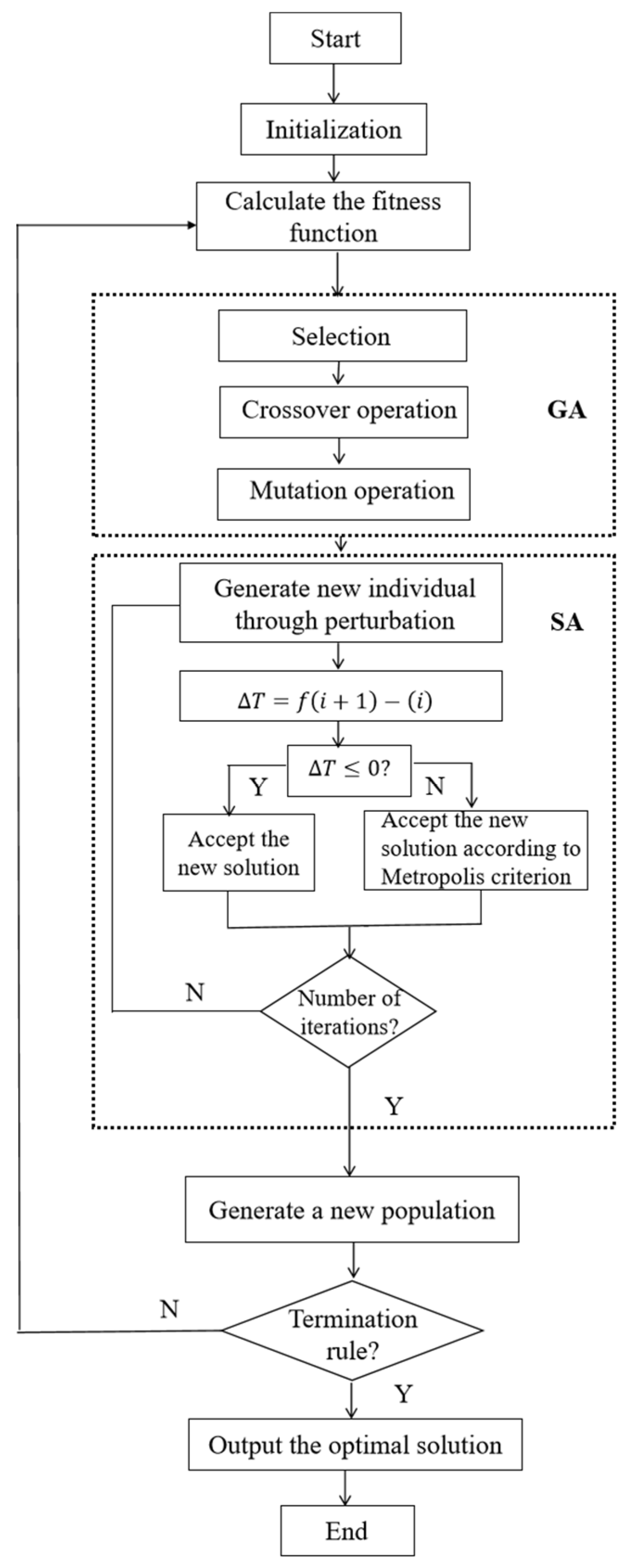
5.1. The Design of GA-SA

To address the complexity of the port container transportation network flow allocation problem under demand uncertainty, we propose an improved Genetic Algorithm combined with Simulated Annealing (GA-SA). This hybrid approach leverages the GA’s global search capability while incorporating SA’s ability to escape local optima.

5.1.1. Coding and Initialization

The coding method of solutions directly affects the search efficiency and solution quality of the algorithm. In the GA-SA algorithm, we adopt a two-part coding scheme to represent solutions. This coding can effectively express two types of decision variables: transportation mode selection and freight flow allocation.

The transportation mode selection matrix is represented as an $\left|I\right|\times \left|J\right|\times \left|M\right|$ binary matrix, corresponding to the decision variable $y_{ijm}$. Here, $y_{ijm}=1$ indicates that transportation mode $m$ from LPW $i$ to CP $j$ is selected, and $y_{ijm}=0$ indicates that this transportation mode $m$ is not selected.

The freight flow allocation matrix $\left|I\right|\times \left|J\right|\times \left|M\right|$ is represented as a real-valued matrix, corresponding to the decision variable $x_{ijm}$, which represents the quantity of goods transported from LPW $i$ to CP $j$ via transportation mode $m$.

5.1.2. Fitness Function

In this study, the fitness function directly uses the objective function of the model, that is, to minimize the total expected cost. To handle the constraint conditions, this study adopts the penalty function method, adding the constraint violation degree into the fitness function:

$$F\left(X,Y\right)=f\left(X,Y\right)+{\displaystyle \sum _k{w}_k\cdot \max \left(0,g_k{\left(X,Y\right)}^2\right)}$$

(27)

where $g_k\left(X,Y\right)$ represents the violation degree of the k-th constraint and $w_k$ is the corresponding penalty weight. The calculation of the specific constraint violation degree is as follows:

(1)

The violation degree of the flow balance constraint is $g_1\left(X,Y\right)=\left|{\displaystyle \sum _{i\in I}{\displaystyle \sum _{m\in M}{x}_{ijm}-d_j}}\right|$.

(2)

The violation degree of the transportation mode selection and freight flow matching constraint is $g_2\left(X,Y\right)={\displaystyle \sum _{i\in I}{\displaystyle \sum _{j\in J}{\displaystyle \sum _{m\in M}\max \left(0,x_{ijm}-A\cdot y_{ijm}\right)}}}$, where A is a sufficiently large positive number.

(3)

The violation degree of the chance constraint is $g_3\left(X,Y\right)=\max \left(0,\alpha -P\cdot x_{ijm}\le Ca{p}_{ijm}\right)$.

The choice of penalty weight $w_k$ has a significant impact on the algorithm’s performance. This study adopts an adaptive penalty weight strategy. Initially, a relatively small penalty weight is set, and as the number of iterations increases, the penalty weight gradually increases to balance the feasibility and quality of the solution. The penalty weight update formula is $w_k^{\left(t+1\right)}=w_k^{\left(t\right)}\cdot \left(1+\delta \cdot \mathbf{1}\left(g_k\left(X^{*},Y^{*}\right)>0\right)\right)$, where $\delta$ is the growth coefficient, and $\mathbf{1}\left(\cdot \right)$ is the indicator function, and its value is either 0 or 1. When the current optimal solution $\left(X^{*},Y^{*}\right)$ violates the k-th constraint, the corresponding penalty weight will increase. This design of the adaptive penalty function can effectively guide the algorithm to converge towards the feasible region while maintaining the exploration of high-quality solutions.

5.1.3. Crossover Operation

The crossover operation in GA simulates the process of biological chromosome exchange and is the main means of generating new individuals. Considering the two-part characteristic of the encoding for this problem, different crossover operations are designed for the transportation mode selection matrix and the freight flow allocation matrix.

For the transportation mode selection matrix, a modified two-point crossover operation is adopted. Two crossover points are randomly selected, and the gene segments between these two points of two parent individuals are exchanged. Individuals that may violate the constraint “at least one transportation mode is selected for each OD pair” after crossover are repaired.

The specific repair operation is to check each OD pair $\left(i,j\right)$. If no transportation mode is selected (that is, all $y_{ijm}$ are 0), then a transportation mode $m^{\prime }$ is randomly selected and ${y_{ijm}}^{\prime }$ is set to 1.

For the freight flow allocation matrix, arithmetic crossover is adopted.

$$x_{ijm}^{child1}=\alpha \cdot x_{ijm}^{parent1}+\left(1-\alpha \right)\cdot x_{ijm}^{parent2}$$

(28)

$$x_{ijm}^{child2}=\left(1-\alpha \right)\cdot x_{ijm}^{parent1}+\alpha \cdot x_{ijm}^{parent2}$$

(29)

where $\alpha$ is a randomly generated crossover coefficient, $\alpha \in \left[0,1\right]$. To increase the diversity of solutions, $\alpha$ can be a numerical value or a matrix, generating different crossover coefficients for each $\left(i,j,m\right)$ combination.

After crossover, the freight flow allocation matrix needs to be normalized to ensure that the flow balance constraint is satisfied. The normalization method is

$$x_{ijm}^{norm}=x_{ijm}\cdot {\displaystyle \frac{d_j}{{\displaystyle \sum _{i\in I}{\displaystyle \sum _{m\in M}{x}_{ijm}}}}}$$

(30)

In addition, to improve the efficiency of the crossover operation, this study introduces a heuristic crossover strategy. For the freight flow allocation matrix, the crossover coefficient is adjusted according to the fitness values of the parent individuals.

$$\alpha ={\displaystyle \frac{F\left(\left(X^{parent2},Y^{parent2}\right)\right)}{F\left(\left(X^{parent1},Y^{parent1}\right)\right)+F\left(\left(X^{parent2},Y^{parent2}\right)\right)}}$$

(31)

In this way, parent individuals with better fitness values contribute more to the offspring, which helps to retain superior genes.

5.1.4. Simulated Annealing

To prevent the algorithm from becoming trapped in local optima, this study introduces a Simulated Annealing mechanism, which accepts inferior solutions with a certain probability to enhance the global search ability of the algorithm. In each iteration, for a newly generated individual, if its fitness is superior to that of the current individual, it is directly accepted. If the fitness is inferior, it is accepted according to the following probability:

$$p=\left\{\begin{array}{c}1,if F\left(X_{new},Y_{new}\right)<F\left(X_{old},Y_{old}\right)\\ \exp \left(-{\displaystyle \frac{F\left(X_{new},Y_{new}\right)-F\left(X_{old},Y_{old}\right)}{T}}\right),\mathrm{otherwise}\end{array}\right.$$

(32)

where $T$ is the current temperature, which controls the probability of accepting inferior solutions. The higher the temperature, the greater the probability of accepting inferior solutions, which is beneficial for global search. The lower the temperature, the more the algorithm tends to accept better solutions, which is beneficial for local optimization.

The annealing temperature decreases exponentially:

$$T_{k+1}=\lambda \cdot T_k$$

(33)

where $T_k$ represents the temperature at the k-th iteration and $\lambda \in \left(0,1\right)$ is the cooling coefficient. The choice of the cooling coefficient $\lambda$ is a trade-off. A larger $\lambda$ (close to 1) makes the temperature decrease slowly, enhancing the global search ability but possibly leading to a slow convergence speed. A smaller $\lambda$ makes the temperature drop rapidly, accelerating convergence but possibly becoming trapped in local optima.

This study adopts a segmented cooling strategy, and the cooling coefficient is adjusted according to the solution stage:

$$\lambda =\left\{\begin{array}{c}{\lambda }_1, if \mathrm{t}<{\mathrm{T}}_1\\ {\lambda }_2< if{ \mathrm{T}}_1<\mathrm{t}<{\mathrm{T}}_2\\ {\lambda }_3,if \mathrm{t}>{\mathrm{T}}_2\end{array}\right.$$

(34)

where ${\lambda }_1>{\lambda }_2>{\lambda }_3$, and ${\mathrm{T}}_1$ and ${\mathrm{T}}_2$ are preset iteration thresholds. This segmented cooling strategy can maintain a high global search ability in the initial stage of the algorithm, accelerate convergence in the middle stage, and perform fine-grained local optimization in the later stage.

In addition, to prevent the algorithm from becoming trapped in local optima prematurely, this study also introduces a temperature restart mechanism. When the optimal solution has not improved for multiple consecutive iterations (such as 10 times), the temperature is increased to a certain proportion (such as 50%) of the initial temperature to help the algorithm escape from local optima traps.

5.1.5. Local Search

To accelerate convergence and improve the quality of solutions, this study conducts local searches on the optimal individual after each iteration. The core idea of local search is to conduct small-scale exploration within the neighborhood of the current optimal solution, attempting to further improve the solution quality through local adjustments.

The specific steps of local search are as follows: Randomly select an OD pair $\left(i,j\right)$. Adjust the freight flow allocation among different transportation modes for this OD pair. The specific method is as follows: Select two transportation modes $m_1$ and $m_2$, where $y_{ij{m}_1}=y_{ij{m}_2}=1$. Calculate the adjustable freight flow volume $\mathrm{\Delta }x=\min \left(x_{ij{m}_1},Ca{p}_{ij{m}_2}-x_{ij{m}_2}\right)$. Transfer the freight flow from transportation mode $m_1$ to transportation mode $m_2$. Evaluate the adjusted solution. If it is better, accept the adjustment; otherwise, keep the original solution.

This local search strategy takes advantage of the characteristics of the problem. By reallocating freight flows among different transportation modes, it can quickly find local optimal solutions. To improve the efficiency of local search, heuristic selection can be carried out based on information such as transportation costs and congestion conditions, giving priority to adjusting those OD pairs and transportation modes that are likely to bring greater improvements. In addition, to prevent local searches from falling into a loop, a taboo list can be maintained to record the recently adjusted OD pair and transportation mode combinations, and these combinations will not be considered within a certain period (such as 10 local searches). Experience shows that local search can significantly improve the solution quality and the algorithm’s convergence speed, especially when dealing with large-scale optimization problems with complex local structures. In conclusion, the GA-SA algorithm framework is shown in Figure 2. After completing the description of the optimization strategy for the GA-SA module, the next step is to focus on the specific construction of the DQN module, aiming to further enhance the learning ability of the solution.

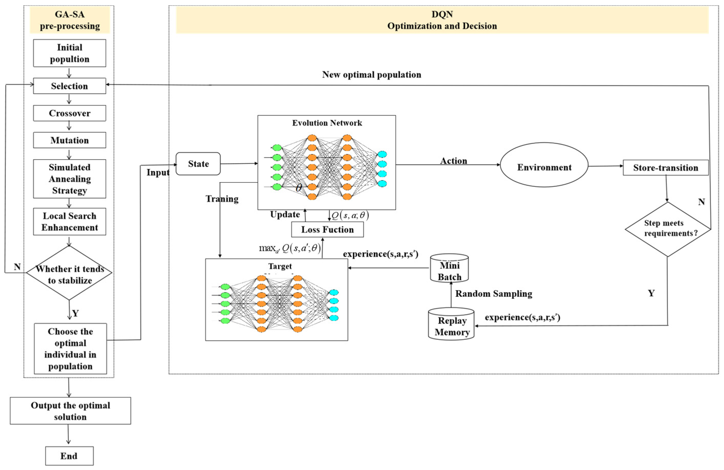
5.2. The Design of DQN

To complement the GA-SA approach, we develop a Deep Q-Network (DQN) reinforcement learning algorithm that can learn optimal flow allocation strategies through interaction with the environment. The DQN approach offers advantages in handling the complex state space and uncertainty in the problem [33,34,35,36,37,38,39].

5.2.1. State Space Design

The design of the state space is key to the application of DQN, as it needs to include all relevant information about the problem while maintaining an appropriate dimensionality for effective learning by the neural network. In this study, the state space $s$ captures the current status of the port transportation network and is defined as a multi-dimensional vector:

$$s=\left\{F,C,E,T,U\right\}$$

(35)

where $F=\left\{f_{ij}^m\right\}$ represents the current flow allocation matrix; $f_{ij}^m$ represents the normalized flow from logistics park warehouse (LPW) $i$ to coastal port (CP) $j$ using mode m; $C=\left\{c_j\right\}$ represents the current congestion level at CP $j$, calculated as the ratio of incoming flow to the port’s capacity; $E=\left\{e_j\right\}$ represents the current carbon emission level at CP $j$, normalized against the emission target; $T=\left\{t_{ij}^m\right\}$ represents the remaining available capacity for each transportation link $\left(i,j,m\right)$; and $U=u_j$ represents the uncertainty factor for each port’s demand, calculated as the ratio of standard deviation to mean demand $\left({\sigma }_j/\overline{D_j}\right)$.

5.2.2. Action Space Design

The action space $A$ consists of discrete decisions to adjust the flow allocation. Each action $a\in A$ is defined as

$$a=\left\{i,j,m,\delta \right\}$$

(36)

where $i\in I$ represents the source LPWs, $j\in J$ represents the destination CPs, $m\in M$ represents the transportation mode, and $\delta \in \left\{{\mathrm{\Delta }}_1,{\mathrm{\Delta }}_2,\dots ,{\mathrm{\Delta }}_k\right\}$ is a set of discrete adjustment values for the flow. This formulation enables the DQN agent to learn which transportation links should be adjusted and the extent of adjustment to optimize the objective function.

5.2.3. Reward Function Design

The reward function is designed to align with the optimization objective while providing immediate feedback for learning. The reward $R$ for transitioning from state $s$ to $s^{\prime }$ after taking action $a$ is defined as

$$R\left(s,a,s^{\prime }\right)=-\mathrm{\Delta }TC-{\beta }_1\cdot \mathrm{\Delta }EC-{\beta }_2\cdot \mathrm{\Delta }CC-{\beta }_3\cdot \mathrm{\Delta }CTSC+{\beta }_4\cdot P_{feas}$$

(37)

where $\mathrm{\Delta }TC$ is the change in transportation cost, $\mathrm{\Delta }EC$ is the change in environmental cost, $\mathrm{\Delta }CC$ is the change in congestion cost, and $\mathrm{\Delta }CTSC$ is the change in carbon tax and subsidy cost. $P_{feas}$ is the feasibility premium that offers a positive reward when the solution becomes more feasible or keeps its feasibility. ${\beta }_1,{\beta }_2,{\beta }_3,{\beta }_4$ are weighting coefficients used to balance different cost components.

5.2.4. Network Architecture and Training

The DQN utilizes a deep neural network to approximate the Q-function. Its architecture is as follows: There is an input layer whose dimensionality corresponds to that of the state space. Then, there are three hidden layers, containing 256, 128, and 64 neurons, respectively, and these layers utilize ReLU activation functions. Finally, there is an output layer with a size equal to the action space, which represents the Q-values for each possible action. This architecture enables the DQN to process the state information from the environment, learn through the hidden layers, and output the estimated Q-values for different actions, enabling the agent to make optimal decisions to maximize cumulative rewards.

The network is trained using experience replay and a target network to stabilize learning. The experience replays buffer stores transitions $\left(s,a,r,s^{\prime }\right)$ and randomly samples batches for training to break the correlation between consecutive samples. The target network parameters are updated periodically from the online network to reduce overestimation bias.

The loss function for training is the mean squared error between the predicted Q-values and the target Q-values:

$$L={\rm E}\left[{\left(r+\gamma \underset{a^{\prime }}{\max Q}\left(s^{\prime },a^{\prime };\overline{\theta }\right)-Q\left(s,a;\theta \right)\right)}^2\right]$$

(38)

where $\theta$ denotes the parameters of the online network, $\overline{\theta }$ represents the parameters of the target network, and $\gamma$ is the discount factor for future rewards.

Check if the number of steps meets predefined requirements. If it meets them (Y), continue the cycle of interacting with the environment, storing experience, and sampling training the network. If not (N), the training may stop or move to the next state.

In summary, the basic framework of DQN is illustrated in Figure 3.

5.3. The Framework of GA-SA-DQN

Based on the definitions of the state, action, and reward functions of DQN in the previous section, we will now organically integrate these two components to construct the hybrid GA-SA-DQN framework, thereby leveraging the advantages of both global search and deep learning. In the first stage, the improved GA-SA algorithm rapidly searches for potential high-quality solution regions from a large-scale solution space by simulating the biological evolution process. The crossover and mutation operations of GA provide extensive exploration capabilities in the solution space, while the probabilistic acceptance mechanism of SA helps the algorithm escape from local optimal traps. The main objective of this stage is to find solutions close to the global optimum, laying the foundation for subsequent fine-tuning optimization.

In the second stage, DQN, as a deep reinforcement learning method, can learn the optimal decision-making strategy through continuous interaction with the environment. In this stage, DQN takes the solutions obtained in the first stage as the initial states and conducts adaptive adjustment and optimization for demand uncertainties through a trial-and-error learning approach. The value function of DQN can evaluate the long-term benefits of different freight flow allocation strategies, thereby finding more robust solutions. The complete algorithm framework is shown in Figure 4.

In summary, this section analyzes the design details of the GA-SA module and the DQN module step by step and finally presents their combined framework. The next section, based on the methods described here, will carry out a systematic evaluation of the algorithm’s performance and compare it with existing approaches.

6. Numerical Experiments

Building on the hybrid algorithm discussed in Section 5, numerical experiments were conducted to evaluate the performance and effectiveness of the proposed approach. The experiments were performed using Python 3.10 on an Intel Quad Core 2.10 GHz processor with 12 GB of memory. These tests aimed to assess the algorithm’s capability in optimizing freight flow distribution in port collection and distribution networks under uncertain demand conditions. The results from the previous theoretical model were applied to real-world data, as detailed in the case study, to validate the robustness and practical utility of the solution.

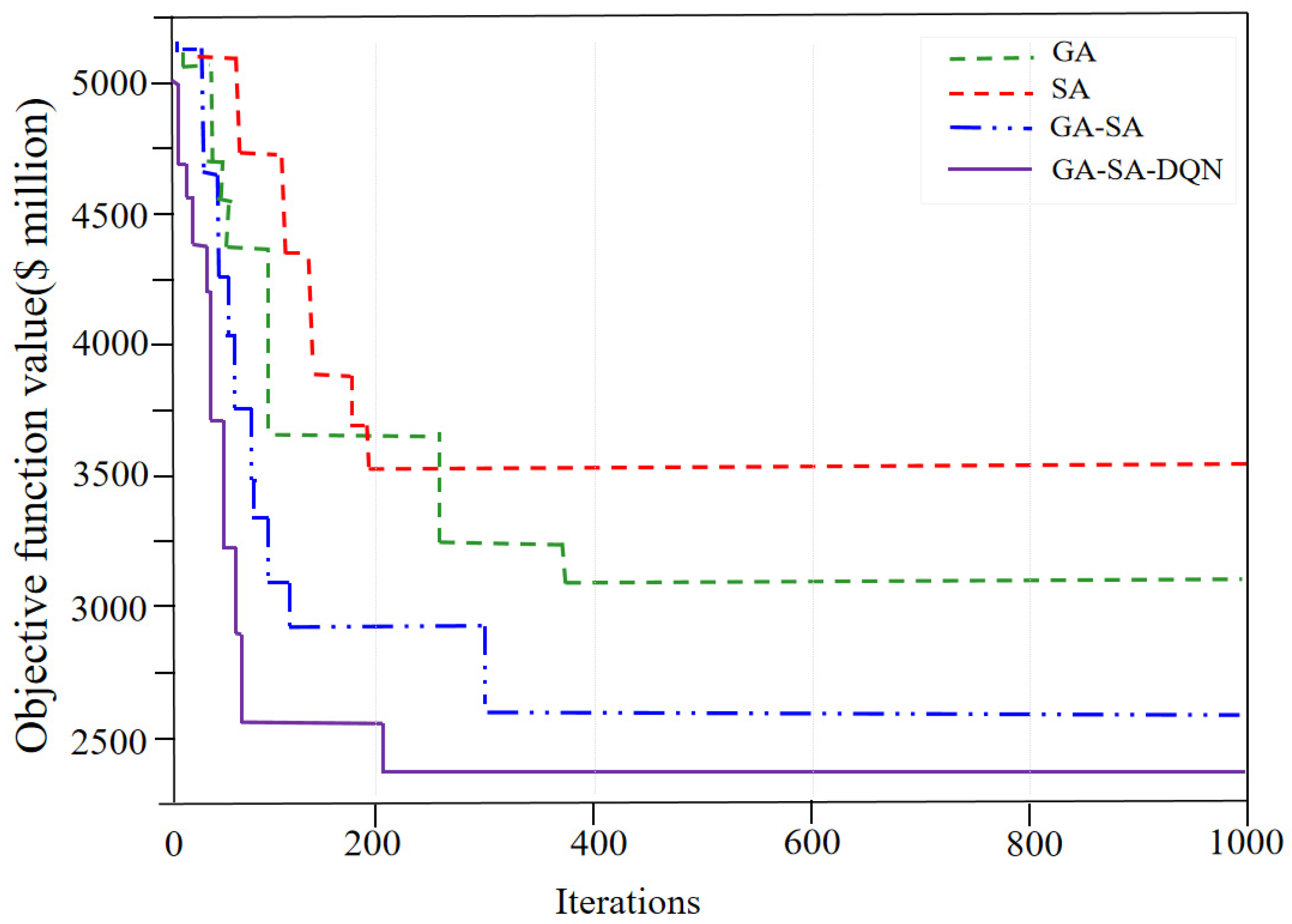
6.1. Algorithm Performance Testing

To comprehensively validate the effectiveness and robustness of the proposed GA-SA-DQN hybrid algorithm, this study designed a series of test instances with different scales and characteristics and compared them with several traditional algorithms.

Table 2. Configuration of test instances.

Instance Number	Number of LPWs	Number of CPs	Number of Transportation Modes
S1	2	2	4
S2	3	2	4
S3	3	3	4
S4	4	2	4
M1	4	3	4
M2	5	3	4
M3	5	4	4
M4	6	4	4
L1	8	4	4
L2	10	4	4
L3	10	5	4
L4	12	6	4

presents the instance configurations used for algorithm performance testing, including instances of different network scales.

The demand data, distance matrix, cost parameters, etc., for each instance were randomly generated based on the characteristics of the actual port collection and distribution system. Meanwhile, sufficient diversity in the parameter distribution among different instances was ensured to test the algorithm’s adaptability in various scenarios. To ensure the reliability of the results, each instance was solved independently 10 times, and the average results were taken for comparative analysis.

The main algorithm parameter settings used in the experiment are shown in

Table 3. The main algorithm parameter settings.

Parameter	Value
population size	100
maximum number of iterations	1000
crossover probability	0.85
mutation probability	0.15
initial temperature	100
cooling rate	0.95
local search probability	0.2
neural network structure	[Input Layer, 256, 128, 64, Output Layer]
learning rate	0.001
discount factor	0.95
experience replay buffer size	10,000
target network update frequency	10
batch size	64
initial value of ε—greedy exploration	1.0
minimum value of ε—greedy exploration	0.01
decay rate of ε—greedy	0.995

.

To comprehensively evaluate the algorithm’s performance, we adopt the following three key indicators: Solution quality is measured by the objective function value (total expected cost), which is compared with the exact solution obtained by CPLEX, and the percentage of relative deviation is calculated. Computational efficiency is measured by the solution time (in seconds), reflecting the running speed of the algorithm. Solution stability is measured by the standard deviation of the objective function values from 10 independent runs, reflecting the stability and reliability of the algorithm’s results.

Table 4. Comparison of algorithm performance for all test instances.

Instance	Algorithm	Objective Function Value (CNY 10,000)	Relative Deviation (%)	Computation Time (Seconds)	Standard Deviation (CNY 10,000)
S1	CPLEX	325.42	-	0.58	0.00
S1	GA	327.85	0.75	3.24	3.15
S1	SA	328.67	1.00	2.87	4.23
S1	GA-SA	326.18	0.23	2.35	1.84
S1	GA-SA-DQN	325.65	0.07	1.98	0.95
S2	CPLEX	428.56	-	0.92	0.00
S2	GA	432.13	0.11	4.56	4.26
S2	SA	433.74	0.73	4.12	5.34
S2	GA-SA	429.87	0.07	3.75	2.13
S2	GA-SA-DQN	429.15	0.13	3.05	1.24
S3	CPLEX	542.67	-	1.25	0.00
S3	GA	548.81	1.13	6.53	5.37
S3	SA	550.42	1.43	5.78	6.85
S3	GA-SA	544.32	0.30	4.67	2.45
S3	GA-SA-DQN	543.28	0.11	3.85	1.28
S4	CPLEX	653.89	-	2.34	0.00
S4	GA	662.57	0.41	8.46	7.24
S4	SA	665.21	0.65	7.65	8.56
S4	GA-SA	656.35	0.08	6.23	3.65
S4	GA-SA-DQN	654.72	0.58	5.12	1.87
M1	CPLEX	762.34	-	12.56	0.00
M1	GA	776.52	1.27	24.78	8.45
M1	SA	780.15	1.05	22.35	10.27
M1	GA-SA	768.53	0.04	16.42	5.32
M1	GA-SA-DQN	764.68	0.55	14.28	3.15
M2	CPLEX	865.27	-	26.34	0.00
M2	GA	883.75	2.14	35.67	11.28
M2	SA	886.92	2.50	32.45	13.56
M2	GA-SA	872.43	0.25	22.37	6.75
M2	GA-SA-DQN	868.56	0.38	18.64	4.23
M3	CPLEX	967.32	-	38.76	0.00
M3	GA	989.85	3.03	42.34	14.56
M3	SA	994.27	0.66	39.65	16.32
M3	GA-SA	976.24	0.66	25.48	8.83
M3	GA-SA-DQN	971.53	0.17	21.74	5.26
M4	CPLEX	1124.56	-	65.23	0.00
M4	GA	1153.28	1.48	68.52	18.74
M4	SA	1159.75	2.05	64.37	21.45
M4	GA-SA	1136.48	0.004	42.36	11.24
L1	CPLEX	1856.43	-	428.75	0.00
L1	GA	1932.56	3.17	165.34	32.56
L1	SA	1945.23	1.97	153.27	38.42
L1	GA-SA	1885.27	0.52	123.45	21.35
L1	GA-SA-DQN	1868.34	0.37	98.76	12.45
L2	CPLEX	2124.68	-	765.42	0.00
L2	GA	2228.54	2.07	214.56	45.78
L2	SA	2246.82	1.16	198.35	52.34
L2	GA-SA	2162.37	0.41	156.43	28.53
L2	GA-SA-DQN	2138.75	0.21	124.85	15.23
L3	CPLEX	2356.85	-	1245.67	0.00
L3	GA	2485.46	3.16	256.78	54.85
L3	SA	2508.32	1.73	238.45	63.62
L3	GA-SA	2402.56	0.32	184.32	32.34
L3	GA-SA-DQN	2372.43	0.24	145.63	18.76
L4	CPLEX	2845.32	-	2856.45	0.00
L4	GA	3126.78	9.9	342.56	74.35
L4	SA	3658.24	28.6	318.67	85.24
L4	GA-SA	2608.67	8.3	242.85	42.56
L4	GA-SA-DQN	2467.85	13.3	187.42	24.35

shows the comparison results of the algorithm performance for all test instances.

As can be seen from Table 4, the performance differences among the algorithms gradually increase as the instance size increases. For smaller instance sizes (e.g., S1–S4), the differences among the algorithms are relatively small, but GA-SA-DQN always maintains the minimum solution bias and high computational efficiency. When the instance size increases (e.g., M1–M4 and L1–L4), the advantages of GA-SA-DQN become more obvious, especially in terms of solution quality and computation time.

For the largest L4 instance (12 LPWs, 6 CPs, and 4 modes of transportation), CPLEX takes about 47 min to obtain the exact solution, while GA-SA-DQN takes only about 3 min to obtain a solution that is less than 1% different from the exact solution, which is a reduction of computation time by about 93%. Also, the solution stability of GA-SA-DQN (USD 243,500 standard deviation) is significantly better than the other heuristics (USD 743,500 for GA and USD 852,400 for SA).

Figure 5 presents a comparison of the iterative processes of the various algorithms for the L4 problem instance. As observed, the GA-SA-DQN consistently outperforms the other methods by rapidly converging to a stable solution with minimal fluctuation in the objective function value, reinforcing its computational efficiency and reliability.

6.2. Case Study

This paper selects A Port as a case study to examine the application of the proposed model and algorithm for a port transportation system. A Port is one of the largest container CPs in the world, with a container throughput of 47.57 million TEU in 2023 and a record-breaking 51.51 million TEU in 2024, marking an 8.3% increase. Its transportation system includes multiple port areas and inland logistics nodes, with a large throughput and significant transportation demand uncertainty, making it an ideal case for model validation. The case study focuses on A Port’s main port areas and surrounding LPWs, including four port areas and five major LPWs. The transportation modes include road, rail, water, and the planned underground logistics system.

The main research parameters are sourced as follows:

(1)

Transportation demand data: Estimated based on A Port’s daily container throughput of 141,000 TEU in 2024.

(2)

Distance data: Measured through electronic maps for the actual transportation distances between LPWs and CPs areas, considering the impact of newly opened highways.

(3)

Transportation costs: Referencing the 2024 Shanghai transport price guidelines and the impact of fuel price fluctuations.

(4)

Carbon emission factors: Using recommended values from the Transportation Industry Carbon Emission Calculation Methodology.

(5)

Underground logistics system parameters: Based on data from the 2023–2024 Shanghai Urban Underground Space Research Institute.

The main parameters and the distance data for the major OD pairs in A Port will be presented next.

To comprehensively evaluate the effectiveness of the proposed model and algorithm, three scenarios were designed for comparison:

Scenario A

(traditional scenario): Only considers road, rail, and water transportation modes, excluding an underground logistics system, and aims to minimize transportation costs.

Scenario B

(environmentally prioritized scenario): Incorporates underground logistics system but excludes demand uncertainty, aiming to minimize total costs (including transportation, environmental, carbon tax and subsidy, and congestion costs).

Scenario C

(proposed scenario): Includes an underground logistics system and accounts for demand uncertainty, aiming to minimize expected total costs.

6.2.1. Total Cost Analysis

The total cost comparison of the three scenarios is shown in

Table 5. Total cost comparison of each scenario (unit: 10,000 CNY/day).

Cost Category	Scenario A	Scenario B	Scenario C
Transportation Cost	4562.8	4285.3	4318.6
Environmental Cost	783.5	498.2	512.7
Congestion Cost	625.4	267.8	293.2
Carbon Tax/Subsidy Cost	143.2	79.5	85.3
Total Cost	6114.9	5130.8	5209.8
Reduction Compared to Scenario A	-	16.1%	14.8%

.

In terms of cost structure, transportation costs accounted for the largest proportion of total costs in each scenario, followed by environmental costs and congestion costs. The total costs of Scenario B and Scenario C are reduced by 16.1% and 14.8%, respectively, compared to Scenario A, indicating that the introduction of an underground logistics system significantly reduces the total costs of the port consolidation and transportation system.

It is particularly noteworthy that the improvements in environmental and congestion costs are particularly significant for Scenarios B and C, with reductions of about 36.4% and 57.2% (Scenario B) and 34.6% and 53.1% (Scenario C), respectively. This suggests that underground logistics systems play an important role in reducing environmental costs (i.e., minimizing CO₂, NO_x, SO_x, and particulate matter emissions) and alleviating congestion. These improvements arise because the underground logistics system shifts a substantial share of short-haul, high-frequency container movements off crowded roadways and into a dedicated, electric-driven pipeline: by replacing diesel-powered trucks with continuous-flow vehicles, local air pollutants and greenhouse gas emissions fall sharply, and the need for curbside loading and unloading is all but eliminated. Consequently, road capacity during peak hours is freed up, average travel times become more predictable, and overall system resilience is enhanced. Moreover, the consolidation of cargo flows in the underground network reduces wear and tear on surface infrastructure and lowers accident risks, yielding downstream savings in maintenance and liability.

Meanwhile, Scenario C’s total cost is only about 1.5% higher than Scenario B’s because, under demand uncertainty, the model deliberately retains a slightly larger share of flexible road transport capacity to buffer against throughput fluctuations. This modest increase reflects an adaptive strategy that, although it incurs marginally higher costs, ensures robust service levels during demand spikes and thus guarantees more reliable port operations in practice. This finding confirms that the model, under conditions of demand uncertainty, can simultaneously reduce overall operational costs, alleviate congestion, and uphold environmental benefits, thereby fulfilling the study’s original objectives.

6.2.2. Cargo Flow Distribution Results

Table 6. Distribution ratios of freight flows for different transportation modes under various scenarios.

Transportation Mode	Scenario A	Scenario B	Scenario C
Road	68.5%	37.2%	40.4%
Railway	15.8%	12.5%	13.2%
Waterway	15.7%	10.3%	11.4%
Underground Logistics System	0.0%	40.0%	35.0%
Total	100.0%	100.0%	100.0%

shows the distribution ratios of freight flows for different transportation modes under three scenarios.

As can be seen from the results of cargo flow distribution, road transportation dominates in Scenario A, with a high proportion of 68.5%, while railroads and waterways account for 15.8% and 15.7%, respectively. After the introduction of the underground logistics system, the proportion of road transportation in Scenario B and Scenario C drops to 37.2% and 40.4%, respectively, while the UCLS accounts for 40.0% and 35.0%. This eases congestion around the port. Queues shrink. Speeds rise. Fewer breakdowns cut accident and repair costs. Rail and water shares drop slightly. They lose short-haul loads to the UCLS, not due to lower efficiency. It is worth noting that after considering demand uncertainty (Scenario C), the proportion of road transportation is slightly higher than that without considering demand uncertainty (Scenario B), while the proportion of the underground logistics system is slightly lower. This suggests that in the face of demand uncertainty, road transport is preferred due to its flexibility, while the underground logistics system is more suited to stable and predictable transportation demand.

Overall, the case studies show that the introduction of an underground logistics system can significantly improve the economic and environmental performance of port consolidation systems, even when demand uncertainty is taken into account. By optimizing the distribution of cargo flows between different modes of transport, the underground logistics system can effectively reduce total costs, carbon emissions, and traffic congestion and improve the overall efficiency and sustainability of the system.

This shift in modal share demonstrates that optimizing multimodal transport can markedly ease port-area congestion and boost operational efficiency. For port operators, it is therefore advisable to roll out the ULCS in staged phases—prioritizing deployment when costs remain manageable to free up surface capacity—while retaining a measured level of road transport reserve to handle demand surges and ensure service continuity and leveraging carbon-pricing incentives under supportive policies to drive more cargo onto the low-carbon ULCS.

6.3. Sensitivity Analysis

In order to deeply analyze the impact of each key parameter on the model results, this section conducts a sensitivity analysis, which mainly includes the impact of transportation cost changes, carbon emission factors, demand uncertainty, and low-carbon-ratio requirements.

6.3.1. Impact of Transportation Cost Changes

Transportation cost is one of the key factors affecting cargo flow distribution. This section analyzes the impact of changes in the unit transportation cost of various transportation modes on the cargo flow distribution. Figure 6 demonstrates the impact of changes in underground logistics system costs on cargo flow distribution.

From Figure 6, it is clear that as the cost of the underground logistics system increases, the proportion of cargo flow allocated to it decreases. With regard to road transportation, as the percentage of cost increase of the underground logistics system climbs gradually from 0 to 40%, the proportion of its transportation shows a slow increase, starting at about 40% and approaching 55% when the cost increases to 40%, which means that the cost of the underground logistics system rises, and more goods will tend to be transported by road transportation, and the status of road transportation in the distribution of cargo flow is also gradually improved. The proportion of rail transportation is almost stable in the whole process and always stays between 13 and 15%, which indicates that the change in the cost of the underground logistics system has little influence on the distribution of rail transportation, and the proportion of cargoes choosing rail transportation is basically not disturbed by it. The proportion of water transportation also remains stable, always at a low level of 8–9%, without significant fluctuations due to the increase in the cost of the underground logistics system, indicating that water transportation is minimally affected by changes in its cost.

When the percentage of cost increase starts to rise from 0, the total proportion of the underground logistics system’s cargo flow distribution decreases significantly, starting at about 37%, and then decreases to about 22% when the cost increases to 40%, and when the cost increases to about 25%, the decreasing trend is more prominent. This shows that an increase in the cost of the underground logistics system will significantly reduce its share in the distribution of cargo flow, and as the cost rises, its use for cargo transportation will gradually reduce.

Overall, the impact of changes in the cost of underground logistics systems on the distribution of cargo flows is quite significant, with rising costs driving the shift of cargo transportation from underground logistics systems to road transportation, while rail and water transportation are less affected. This reflects the fact that the choice of transportation modes will be dynamically adjusted, driven by cost factors, with road transportation being more resilient to cost changes and the underground logistics system being less competitive when costs rise. In practice, if the construction cost of the underground logistics systems rises significantly, operators are advised to implement it in stages and use large-scale bidding to reduce unit costs; when costs are under control, they should accelerate rollout to maximize operational returns.

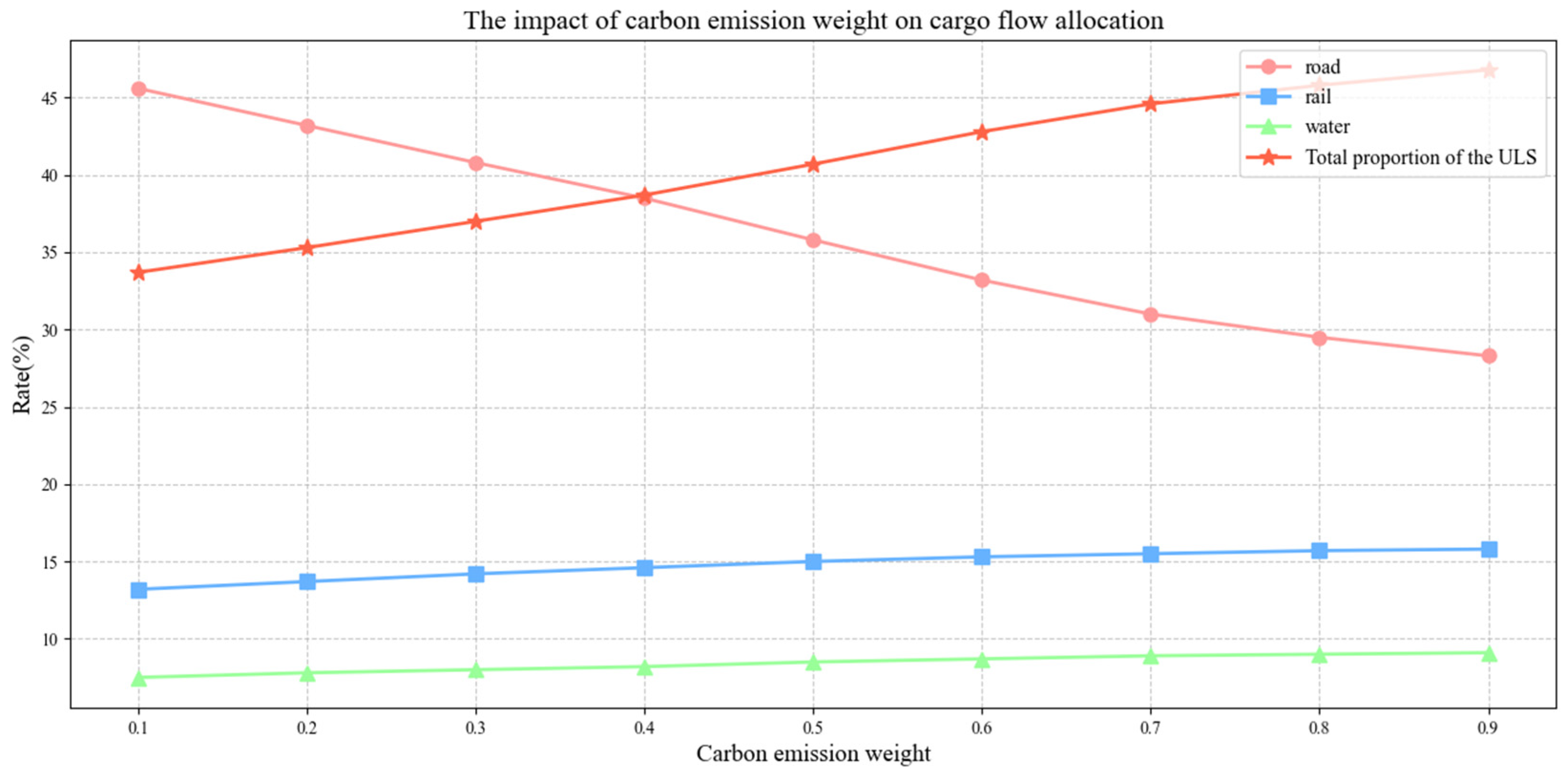
6.3.2. Impact of Carbon Emission Weightings

The carbon emission coefficient directly affects environmental costs and, in turn, influences cargo flow distribution decisions. Figure 7 shows the changes in cargo flow distribution across transportation modes under different carbon emission weightings.

From Figure 7, it can be seen that as the carbon emission weight increases (i.e., the share of environmental costs in total costs rises), the proportion of cargo flow allocated to the underground logistics system and rail/water transport gradually increases, while the proportion allocated to road transport decreases significantly. In particular, when the carbon emission weight increases from 0.1 to 0.5, the proportion of cargo flow allocated to the underground logistics system increases from 33.7% to 40.7%, a rise of 7 percentage points.

Overall, increasing the carbon emission weight positively impacts the promotion of the underground logistics system. In practice, increasing the carbon emission cost weight (e.g., through carbon taxes or carbon trading mechanisms) can effectively promote the development of green, low-carbon transportation modes. The analysis suggests that when the carbon emission weight reaches above 0.3, the underground logistics system will become the dominant transportation mode, which is crucial for developing a green port transportation system. Planners can incorporate a carbon-pricing mechanism into regional low-carbon development plans—linking it to port capacity allocation—so that policy levers drive the adoption of green transportation modes.

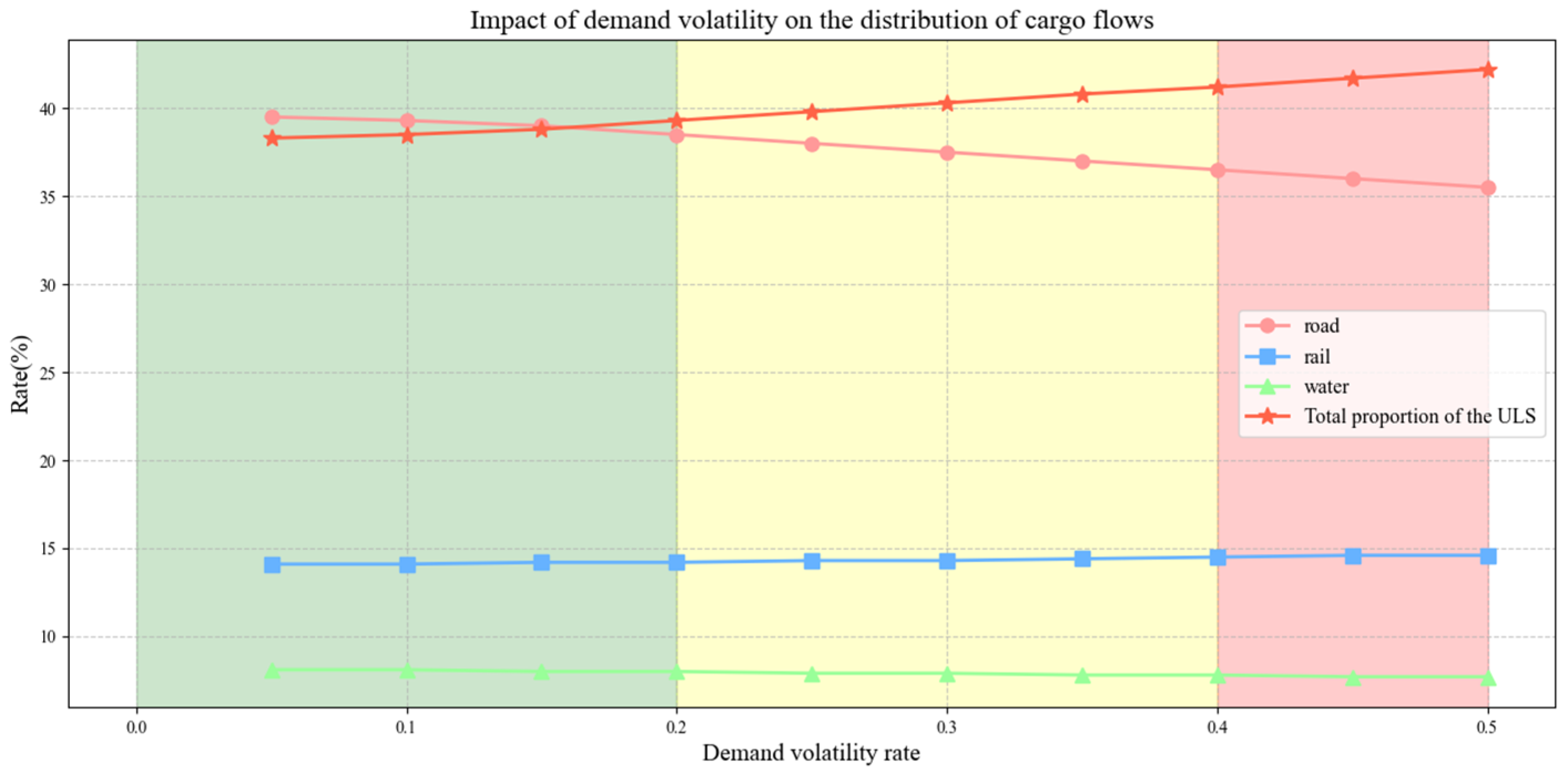
6.3.3. Impact of Demand Uncertainty

The uncertainty of port container demand is an important factor influencing cargo flow distribution strategies. Figure 8 shows the total cost changes under different demand volatility levels.

From Figure 8, it can be observed that as demand volatility increases, total cost increases nonlinearly. When volatility is below 0.2, the cost increases slowly; between 0.2 and 0.4, the cost growth accelerates; and when volatility exceeds 0.4, the cost growth slows down again. This nonlinear relationship indicates that for medium levels of demand uncertainty, the system requires more adjustments to maintain performance, leading to a more significant cost increase.

Figure 9 further demonstrates the changes in cargo flow distribution across different transportation modes under varying demand volatility levels.

From Figure 9, it can be seen that with the increase in demand volatility, the proportion of freight transported by the underground logistics system rises steadily from 38.3% to 42.2%, which shows a good adaptability to volatility. In contrast, the share of road transportation decreases gradually, indicating that it faces certain bottlenecks when demand uncertainty increases. This trend suggests that under high demand volatility, the underground logistics system, with its closed operation, high automation, and dispatch stability, is a more reliable transportation option, especially suitable for securing critical materials and core routes. Port schedulers should establish multiple capacity contingency plans and dynamically adjust the balance between the underground logistics system and road transport, ensuring stable service even when demand fluctuates.

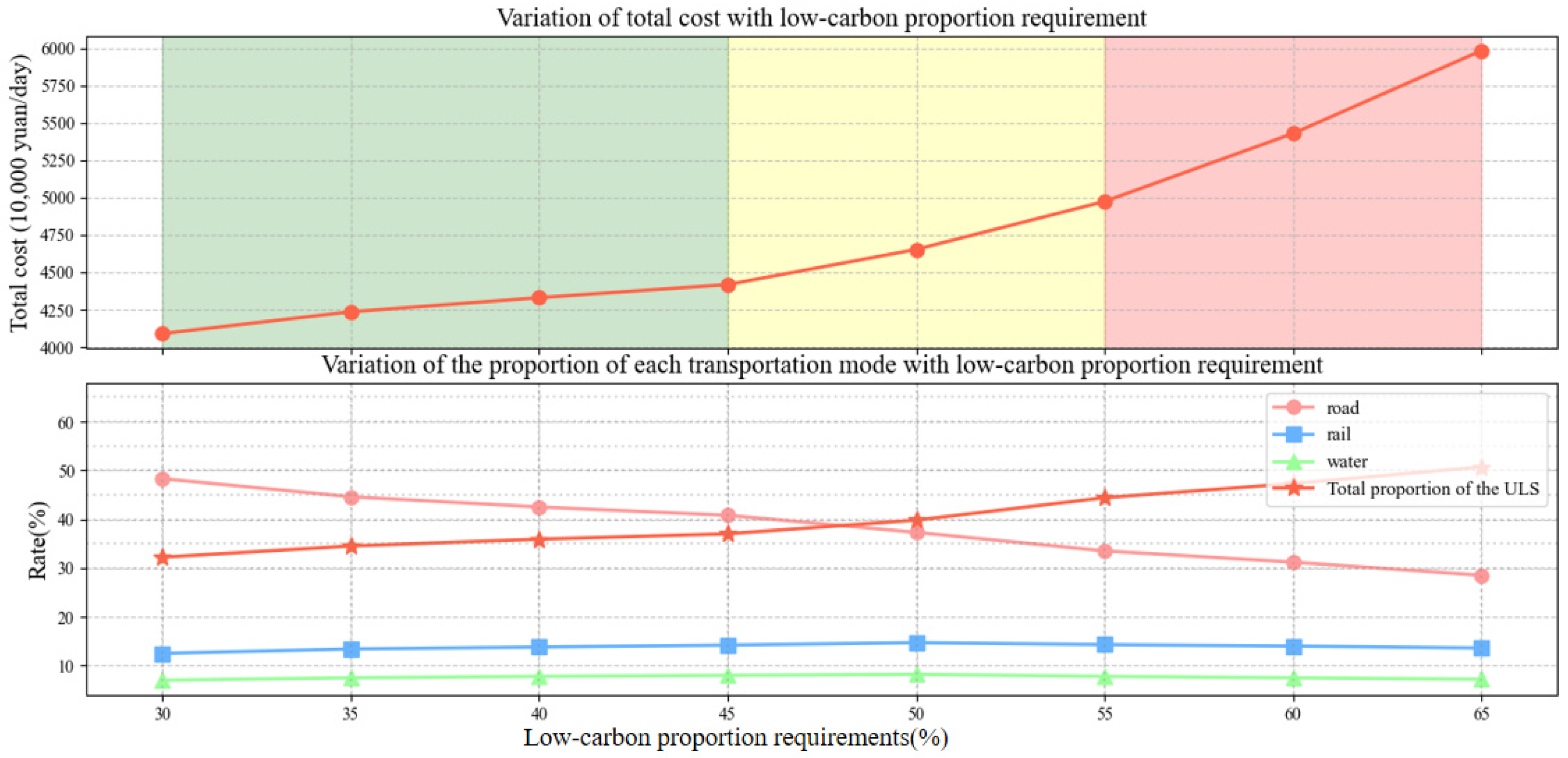
6.3.4. Impact of Low-Carbon-Proportion Requirements

The low-carbon-proportion constraint is an important parameter in the model, directly influencing the cargo flow distribution across transportation modes. Figure 10 shows the cost and cargo flow distribution changes under different low-carbon-proportion requirements.

From Figure 10, it can be seen that as the low-carbon-proportion requirement increases, total costs rise in a stepwise manner. When the requirement increases from 30% to 45%, the cost increases relatively slowly, by about 7.4%. However, when the requirement exceeds 50%, the cost increases significantly, indicating that the system faces greater challenges in adapting to high low-carbon-proportion requirements.

In terms of cargo flow distribution, as the low-carbon-proportion requirement increases, the cargo flow proportion for the underground logistics system increases linearly, from 32.2% to 50.7%, while the proportion for road transport significantly decreases, from 48.3% to 28.5%. Notably, when the low-carbon-proportion requirement reaches 55% or higher, the proportion for rail and water transport also starts to decrease, indicating that under very high low-carbon requirements, the underground logistics system will replace some traditional low-carbon transportation modes.

Based on the sensitivity analysis, the following key conclusions can be drawn:

(1)

Underground logistics system costs: The cost of an underground logistics system has a significant impact on its adoption. Controlling cost increases to within 25% is crucial for maintaining high usage rates.

(2)

Carbon emission weight: increasing the carbon emission cost weight is an effective way to promote the development of underground logistics systems. When the weight exceeds 0.3, the underground logistics system will become the dominant transportation mode.

(3)

Demand uncertainty: As demand uncertainty increases, the proportion of road transport rises, and the proportion of the underground logistics system slightly decreases. A shallow underground logistics system shows better adaptability.

(4)

Low-carbon-proportion requirements: When the low-carbon-proportion requirement is below 45%, the system can adapt with a relatively small increase in cost. However, when the requirement exceeds 50%, costs rise significantly.

These conclusions provide important insights for the planning and operation of port transportation systems, particularly in terms of determining investment strategies for underground logistics systems, formulating carbon reduction policies, and addressing demand uncertainty. When setting low-carbon targets, a phased, incremental approach should be adopted; initial targets ought to lie within a range that allows a smooth transition, supported by subsidies and incentive policies to create sustainable backing for higher levels of green transformation.

7. Conclusions

This study makes three key contributions to the optimization of port cargo flow under uncertainty. First, by embedding an underground container-pipeline logistics system (UCLS) into a stochastic chance-constrained model, we provide a novel framework that simultaneously balances transportation costs, environmental impacts, congestion effects, and carbon tax/subsidy policies—extending beyond the largely deterministic, surface-only approaches in previous research. Second, our hybrid GA-SA-DQN algorithm not only accelerates convergence on large-scale instances but also delivers robust, high-quality solutions under demand volatility, outperforming both CPLEX and classic metaheuristics in runtime and stability. Third, through the empirical case of Port A, we quantify the economic–environmental co-benefits of UCLS: a 16% reduction in total cost, an over 34% cut in environmental expense, and a 53% decline in congestion cost, while maintaining operational resilience even when demand fluctuates.

Despite the contributions outlined above, our model makes several simplifying assumptions that should be addressed in future research. For example, the model omits handling costs, such as the costs associated with loading and unloading goods at transfer points, which can significantly impact the total cost in real-world port operations. Furthermore, transfer costs between different transportation modes (such as truck-to-rail or rail-to-ship transfers) are not considered in our analysis. These costs could influence the optimal cargo flow distribution, especially in multimodal systems where coordination between modes is essential.

Future research should explore the inclusion of handling and transfer costs, as these factors play a crucial role in the efficiency of port operations. Incorporating these costs would provide a more accurate and comprehensive model, better reflecting the complexities of multimodal logistics systems. Additionally, multi-objective optimization frameworks that account for these costs, along with environmental and economic factors, could further enhance the practical applicability and robustness of the model in real-world scenarios.

References

1. UNCTAD. Review of Maritime Transport 2024; United Nations: Geneva, Switzerland, 2024; Available online: https://unctad.org/publication/review-maritime-transport-2024 (accessed on 10 May 2025).
2. UNCTAD. Global Trade Hits Record $33 Trillion in 2024, Driven by Services and Developing Economies. 2025. Available online: https://unctad.org/news/global-trade-hits-record-33-trillion-2024-driven-services-and-developing-economies (accessed on 10 May 2025).
3. Panahi, R.; Ng, A.K.Y.; Afenyo, M.; Lau, Y.Y. Implications of a pandemic outbreak risk: A discussion on China’s emergency logistics in the era of Coronavirus Disease 2019 (COVID-19). J. Int. Logist. Trade 2022, 20, 127–135. [Google Scholar] [CrossRef]
4. Zhao, Z.; Shen, M.; Chen, J.; Wang, X.; Wan, Z.; Hu, X.; Liu, W. Design and optimization of the collaborative container logistics system between a dry port and a water port. Comput. Ind. Eng. 2024, 198, 110654. [Google Scholar] [CrossRef]
5. Acciaro, M.; Arduino, G.; Borruso, G. Port sustainability in the transition to a low-carbon energy system: A review of digital technologies and decarbonization strategies. Transp. Res. Part D Transp. Environ. 2023, 117, 103615. [Google Scholar] [CrossRef]
6. Liu, Q.; Yang, Y.; Li, K.X.; Luo, M.; Xie, C. Liner shipping network vulnerability to component disruptions: A China-Europe container flow analysis. Transp. Res. Part D Transp. Environ. 2024, 131, 104232. [Google Scholar] [CrossRef]
7. Liang, C.; Sun, W.; Shi, J.; Wang, K.; Zhang, Y.; Lim, G. Decarbonizing Maritime Transport through Green Fuel-Powered Vessel Retrofitting: A Game-Theoretic Approach. J. Mar. Sci. Eng. 2024, 12, 1174. [Google Scholar] [CrossRef]
8. Wang, Y.; Liu, Y.; Chen, K.; Zhou, Q. Port hinterland intermodal container transport efficiency and its influencing factors analysis. Transp. Policy 2022, 124, 143–157. [Google Scholar] [CrossRef]
9. Chen, X.; Wei, C.; Xin, Z.; Zhao, J.; Xian, J. Ship Detection under Low-Visibility Weather Interference via an Ensemble Generative Adversarial Network. J. Mar. Sci. Eng. 2023, 11, 2065. [Google Scholar] [CrossRef]
10. Hu, X.; Liang, C.; Chang, D.; Zhang, Y. Container storage space assignment problem in two terminals with the consideration of yard sharing. Adv. Eng. Inform. 2021, 47, 101224. [Google Scholar] [CrossRef]
11. Martinez-Moya, J.; Vazquez-Paja, B.; Gimenez-Maldonado, J.A. Energy consumption minimization of a container terminal by the optimization of eco-efficient operational strategies. Energy 2021, 222, 119925. [Google Scholar] [CrossRef]
12. Karam, A.; Jensen, A.J.K.; Hussein, M. Analysis of the barriers to multimodal freight transport and their mitigation strategies. Eur. Transp. Res. Rev. 2023, 15, 43. [Google Scholar] [CrossRef]
13. Intermodal Freight Transportation Market Size Report. 2030. Available online: https://www.grandviewresearch.com/industry-analysis/intermodal-freight-transportation-market-report (accessed on 14 May 2025).
14. Mamatok, Y.; Jin, M. A transportation service network design problem with mixed temporal constraints. Transp. Res. Part E Logist. Transp. Rev. 2022, 160, 102689. [Google Scholar] [CrossRef]
15. Chen, X.; Wu, S.; Shi, C.; Huang, Y.; Yang, Y.; Ke, R.; Zhao, J. Sensing Data Supported Traffic Flow Prediction via Denoising Schemes and ANN: A Comparison. IEEE Sens. J. 2020, 20, 14317–14328. [Google Scholar] [CrossRef]
16. Liu, Q.; Hu, W.; Dong, J.; Yang, K.; Ren, R.; Chen, Z. Cost-benefit analysis of road-underground co-modality strategies for sustainable city logistics. Transp. Res. Part D Transp. Environ. 2025, 139, 104585. [Google Scholar] [CrossRef]
17. Zhu, L.; Li, W.; Sun, Z.B.; Chen, Y.; Chen, C.; Zhang, L.Y. Evaluating resilience in maritime port and shipping operations under various disruptions: A literature review. Marit. Econ. Logist. 2023, 25, 181–208. [Google Scholar] [CrossRef]
18. van Twiller, J.; Adulyasak, Y.; Delage, E.; Grbic, D.; Jensen, R.M. Navigating Demand Uncertainty in Container Shipping: Deep Reinforcement Learning for Enabling Adaptive and Feasible Master Stowage Planning. arXiv 2025, arXiv:2502.12756. [Google Scholar] [CrossRef]
19. Toygar, A.; Yildirim, U.; Inegöl, G.M. Investigation of empty container shortage based on SWARA-ARAS methods in the COVID-19 era. Eur. Transp. Res. Rev. 2022, 14, 8. [Google Scholar] [CrossRef] [PubMed]
20. Liu, J.; Dong, C.; Li, S. Container shipping network optimization considering underground container transportation. Marit. Policy Manag. 2022, 49, 389–409. [Google Scholar] [CrossRef]
21. Liu, Y.; Feng, B.; Zhu, Y. Underground logistics network design: A review and bibliometric analysis. Transp. Res. Part E Logist. Transp. Rev. 2023, 171, 102978. [Google Scholar]
22. Hu, W.; Dong, J.; Ren, R.; Chen, Z. Underground logistics systems: Development overview and new prospects in China. Front. Eng. 2023, 10, 354–359. [Google Scholar] [CrossRef]
23. Liang, C.; Hu, X.; Shi, L.; Fu, H.; Xu, D. Joint dispatch of shipment equipment considering underground container logistics. Comput. Ind. Eng. 2022, 165, 16. [Google Scholar] [CrossRef]
24. Li, F.; Yuen, K.F. A systematic review on underground logistics system: Designs, impacts, and future directions. Tunn. Undergr. Space Technol. 2025, 159, 106483. [Google Scholar] [CrossRef]
25. Hou, L.; Hu, W.; Chen, Y.; Dong, J.; Ren, R.; Chen, Z. Measuring Effectiveness of Metro-Based Underground Logistics System in Sustaining City Logistics Performance During Public Health Emergencies: A Case Study of Shanghai. Transp. Res. Rec. 2024, 2678, 724–748. [Google Scholar] [CrossRef]
26. Sun, X.; Hu, W. Multi-objective optimization model for planning metro-based underground logistics system network: Nanjing case study. J. Ind. Manag. Optim. 2023, 19, 2607–2635. [Google Scholar] [CrossRef]
27. Xia, N.; Jing, Y.; Wang, W.; Shi, L. Assessment of the carbon emissions and energy efficiency of container terminal: An empirical analysis from China. Sci. Rep. 2021, 11, 1728. [Google Scholar] [CrossRef]
28. Chen, Z.; Hu, W.; Xu, Y.; Dong, J.; Yang, K.; Ren, R. Exploring decision-making mechanisms for the metro-based underground logistics system network expansion: An example of Beijing. Tunn. Undergr. Space Technol. 2023, 139, 105240. [Google Scholar] [CrossRef]
29. An, N.; Yang, K.; Chen, Y.; Yang, L. Wasserstein distributionally robust optimization for train operation and freight assignment in a metro-based underground logistics system. Comput. Ind. Eng. 2024, 192, 110228. [Google Scholar] [CrossRef]
30. Wandel, S.; Anderberg, S.; Larsson, F.E.; Johnsson, A.; Wells, A. Underground capsule pipeline logistic system Feasibility study of an urban application. Transp. Res. Procedia 2023, 72, 3126–3133. [Google Scholar] [CrossRef]
31. Hou, L.; Xu, Y.; Ren, R.; Yang, J.; Su, L. Optimization of three-dimensional urban underground logistics system alignment: A deep reinforcement learning approach. Comput. Ind. Eng. 2025, 205, 111185. [Google Scholar] [CrossRef]
32. Gong, D.; Tian, J.; Hu, W.; Dong, J.; Chen, Y.; Ren, R.; Chen, Z. Sustainable Design and Operations Management of Metro-Based Underground Logistics Systems: A Thematic Literature Review. Buildings 2023, 13, 1888. [Google Scholar] [CrossRef]
33. Vallidevi, K.; Jothi, S.; Karuppiah, S.V. HO-DQLN: Hybrid optimization-based deep Q-learning network for optimizing QoS requirements in service oriented model. Expert Syst. Appl. 2023, 227, 120188. [Google Scholar] [CrossRef]
34. Kim, S.; Jang, M.-G.; Kim, J.-K. Process design and optimization of single mixed-refrigerant processes with the application of deep reinforcement learning. Appl. Therm. Eng. 2023, 223, 120038. [Google Scholar] [CrossRef]
35. Xu, N.; Shi, Z.; Yin, S.; Xiang, Z. A hyper-heuristic with deep Q-network for the multi-objective unmanned surface vehicles scheduling problem. Neurocomputing 2024, 596, 127943. [Google Scholar] [CrossRef]
36. Xue, F.; Hai, Q.; Dong, T.; Cui, Z.; Gong, Y. A deep reinforcement learning based hybrid algorithm for efficient resource scheduling in edge computing environment. Inf. Sci. 2022, 608, 362–374. [Google Scholar] [CrossRef]
37. Zhang, J.; Cheng, L.; Liu, C.; Zhao, Z.; Mao, Y. Cost-aware scheduling systems for real-time workflows in cloud: An approach based on Genetic Algorithm and Deep Reinforcement Learning. Expert Syst. Appl. 2023, 234, 120972. [Google Scholar] [CrossRef]
38. Zhao, F.; Liu, Y.; Zhu, N.; Xu, T.; Jonrinaldi. A selection hyper-heuristic algorithm with Q-learning mechanism. Appl. Soft Comput. 2023, 147, 110815. [Google Scholar] [CrossRef]
39. Liu, X.; Qiu, L.; Fang, Y.; Wang, K.; Li, Y.; Rodríguez, J. Event-Driven Based Reinforcement Learning Predictive Controller Design for Three-Phase NPC Converters Using Online Approximators. IEEE Trans. Power Electron. 2024, 40, 4914–4926. [Google Scholar] [CrossRef]
Figure 1. Schematic diagram of port collection and distribution network considering underground container logistics.
Jmse 13 01173 g001
Figure 2. Flowchart of improved GA-SA.
Jmse 13 01173 g002
Figure 3. The basic framework of DQN.
Jmse 13 01173 g003
Figure 4. The hybrid algorithm framework based on GA-SA-DQN.
Jmse 13 01173 g004
Figure 5. Comparison of algorithmic iterative processes for L4 problem instances.
Jmse 13 01173 g005
Figure 6. Influence analysis of the cost change of the underground logistics system.
Jmse 13 01173 g006
Figure 7. Influence analysis of carbon emission weighting.
Jmse 13 01173 g007
Figure 8. Influence analysis of demand uncertainty.
Jmse 13 01173 g008
Figure 9. Influence analysis of the impact of different demand volatility rates on the freight flow.
Jmse 13 01173 g009
Figure 10. Influence analysis of the impact of changes in costs and freight flow allocation under different low-carbon-proportion requirements.
Jmse 13 01173 g010