A Salvage Target Tracking Algorithm for Unmanned Surface Vehicles Combining Improved Line-of-Sight and Key Point Guidance

Abstract

Surface target salvage is a crucial component of marine emergencies. Although unmanned surface vehicles (USVs) have emerged as effective alternative platforms to traditional artificial salvage, salvage target tracking remains a challenging issue. Therefore, this paper proposes a salvage target tracking (STT) algorithm which enables rapid approach (RA) to the salvage target, while maintaining an appropriate salvage distance that keeps the surface target within the operational range in the terminal tracking (TT) phase. In the RA phase, the model predictive line-of-sight (PLOS) guidance algorithm is proposed to estimate and compensate for the drift angle encountered when following a curved path. In the TT phase, a guidance algorithm based on the key point is proposed to track the salvage target. To achieve the goals in the RA phase and the TT phase, a heading and speed controller based on proportional–integral–derivative control is proposed to track the desired signals computed by the PLOS and key point guidance algorithms. To verify the effectiveness of the STT algorithm, simulation analysis is conducted for the PLOS guidance algorithm and key point guidance algorithm. The simulation results show that the proposed PLOS guidance algorithm has the lowest cross-tracking error compared with the traditional LOS, integral LOS, and adaptive error constraint LOS. Moreover, the distance between the USV and the salvage target is less than the operating radius of the salvage operation. The results demonstrate that the proposed STT algorithm is capable of maintaining the appropriate salvage distance while tracking the salvage target.

1. Introduction

Salvage operations have gained significant importance in contemporary maritime safety management with the increasing frequency of maritime traffic accidents [1,2,3]. Following maritime accidents, salvage operations must be conducted for the ship wreckage and overboard personnel. Applying unmanned surface vehicles (USVs) to salvage sunken objects or people in the water can contribute to reducing personnel costs, enhancing personnel safety, and broadening the operational weather window [4].

Salvage operations with a twin-propeller and non-rudder (TPNR) ship can be conducted by controlling the rotational speed of the two propellers [5]. Since the controller is solely responsible for managing the rotational velocities of the dual propellers, a significant number of USVs employ a TPNR configuration. As the TPNR configuration is prevalent among USVs, the development of a salvage target tracking algorithm specifically designed for TPNR USVs is of paramount importance. However, there are two technical challenges in tracking the salvage target. On the one hand, the unmanned surface vehicle (USV) must ensure precise path-following accuracy when tracking the salvage target at high speed. However, when the USV follows a path at high speed, this can lead to significant path-following errors [6]. On the other hand, there are constraints on the position of the USV relative to the salvage target during the tracking process, as the working space of the salvage actuator needs to cover the salvage target.

Previous studies have investigated the path-following control of USVs, which can be categorized into two categories. The first category is the virtual ship method, where a reference path is generated according to a virtual ship model, and the USV is controlled to follow this path based on the corresponding control algorithm [7]. A low-frequency learning technique based on the virtual ship guidance algorithm was proposed to smooth the reference path [8]. The second category is the fixed coordinate system method, in which the position and course errors are quantified in a coordinate frame. Furthermore, the corresponding controller is designed based on the fixed coordinate system method to reduce errors in the position and course. One of the most widely used systems is the Serret–Frenet coordinate system, which is applicable not only to mobile robot control [9], but also to USV control [10]. These two categories of methods involve the direct design of the controller based on the mathematical model of the path-following system of the USV. The presence of complex nonlinear and uncertain terms in the model will make the design process very difficult [11]. To simplify the design of the controller, Fossen et al. divided the path-following system into a guidance subsystem and a control subsystem [6]. The desired course angle is calculated by the guidance subsystem, and is transmitted to the control subsystem. The control subsystem is responsible for controlling the USV to track the desired course.

The line-of-sight (LOS) guidance algorithm is widely used in guidance subsystems because of its simple design. This algorithm simplifies the design process by focusing solely on the kinematics of the system, thereby reducing the number of parameters to be tuned [12]. Pettersen et al. also proved that the LOS guidance algorithm is globally, uniformly, asymptotically stable [13]. Building on this principle, numerous studies have integrated the LOS guidance algorithm with various heading control methods, such as PID controllers [6], model predictive controllers [14], adaptive controllers, fuzzy logic controllers [15,16], and neural network controllers [17]. However, these heading control methods may result in larger tracking errors because of the low resistance characteristics of the water surface. To address this gap, a nonlinear adaptive state observer is proposed to estimate the drift angle [12]. An improved LOS guidance algorithm based on an extended-state observer is proposed to estimate the time-varying drift angle, which is more realistic than constant drift angle estimation [18].

The improved LOS guidance algorithm enhances path tracking by estimating environmental disturbances, while the USV will converge more quickly after deviating from the path by adjusting the lookahead distance. However, this guidance algorithm uses only a single waypoint, defined as the point on the path nearest to the USV. When the distance between the USV and the waypoint is zero, the desired path calculated by the guidance algorithm is the tangent direction of the path. If the path ahead is curved, the USV will deviate from the path and then be guided back onto the path. Global asymptotic convergence has been proven for the LOS guidance algorithm based on the assumption that the actual course of the USV can be quickly tracked to the desired course [12,18,19]. However, it takes a certain amount of time to track the course, because saturation rate constraints always exist for the propeller and rudder. If the curvature of the path ahead is constantly changing, the direction of the path may change again before the USV converges back to the path. This can lead to significant tracking error. Therefore, it is important to propose a guidance algorithm that can take into account the information of multiple waypoints to reduce the occurrence of the USV deviating from the path.

In the initial research on target tracking technology, target tracking was regarded as an application of path tracking. A path planner was used to generate a path that could reach the target, then path tracking technology was employed to follow the planned path [20,21]. The A-star algorithm was adopted in these studies to generate a path from the USV to the target [22,23]. Singh et al. used the Dijkstra algorithm to generate the desired path [24]. Subsequently, obstacle avoidance became an important consideration in the target tracking process. Some studies began to consider the obstacle avoidance problem during the tracking process. The artificial potential field method is widely used in obstacle avoidance algorithms. Wang et al. proposes a fusion algorithm based on the improved artificial potential field and the collision prediction model to solve the obstacle avoidance problem of wave gliders in the marine environment [25]. Du et al. use a millimeter-wave radar to detect obstacles. When the USV enters the obstacle avoidance area and the yaw angle satisfies certain conditions, it is determined that there is a collision risk, and different guidance algorithms are triggered [26]. Zhang et al. propose an improved artificial potential field algorithm for obstacle avoidance of a dual USV formation to ensure that the two USVs in the formation pass by the same side of the obstacle [27]. Target tracking methods are not limited to realization through path planning. Similarly to path following, line-of-sight guidance and pure pursuit guidance can also be directly applied to the target, instead of being used only on the planned path [4]. Du et al. utilize the line-of-sight angle to design a target tracking control algorithm [26]. In addition, some intelligent control methods, as well as neural network methods, have been applied to target tracking. A vision-based finite-time control method is proposed for an unmanned aerial vehicle to track an uncooperative target in [28]. Aumtab et al. propose a tracking control method based on the fundamental equations of constrained motion with uncertainty control [29]. Liu et al. study the target tracking problem of an underactuated surface vehicle with model uncertainties and external unknown disturbances. A composite, robust, adaptive, self-structuring neural network-bounded controller is proposed to improve system performance and avoid input saturation [30]. Shojaei investigates the three-dimensional target tracking control problem of underactuated autonomous underwater vehicles by using coordinate transformation and multi-layer neural networks [31]. Kim introduces optimal controllers for USV tracking of underwater targets [32].

With the continuous development of technology, USVs are being applied in various scenarios, accompanied by new requirements for target tracking. Kim proposes a tracking mode that encircles the target, thereby achieving all-round monitoring of the target [1]. Du puts forward a target tracking method that uses a constrained line-of-sight angle to enable the USV to better monitor the target [26]. Zhang proposes an algorithm for using a double USV formation to clean up surface debris, requiring two USVs to pass by both sides of the debris, respectively [27]. In addition to avoiding collisions, the target tracking algorithm must ensure that the salvage target remains within the working space of the salvage actuator.

Motivated by the problems mentioned above, this paper studies the salvage target tracking problem for twin-propeller and non-rudder USVs. The main challenges to be addressed include the following: (1) When the USV is tracking the salvage target, it needs to follow the reference path with high precision. Deviations caused by response-time limitations of the USV should be reduced when following a curved path. (2) The USV must maintain a fixed relative positional relationship with the salvage target, ensuring that the salvage target remains on the side of the USV where the salvage actuator is installed. The distance between the salvage target and the USV must be less than the maximum radius of the working space of the salvage actuator. (3) All control objectives can only be achieved by adjusting the rotational speeds of the left and right propellers of the USV.

Therefore, a salvage target tracking algorithm for TPNR USVs is proposed for tracking salvage targets. From a practical perspective, the algorithm is divided into two phases: rapid approach and terminal tracking. When the USV is far from the salvage target, the algorithm is in the rapid approach phase. The model predictive line-of-sight algorithm is applied to track the path from the USV to the salvage target with a high cruising speed and high precision. When the USV is relatively close to the salvage target, the algorithm controls the USV to brake and enter the terminal tracking phase. A guidance algorithm based on the key point is proposed for tracking both stationary and moving salvage targets. The selection of the key point takes into account the installation position of the salvage actuator. The main contributions of the paper can be summarized as follows:

(1)

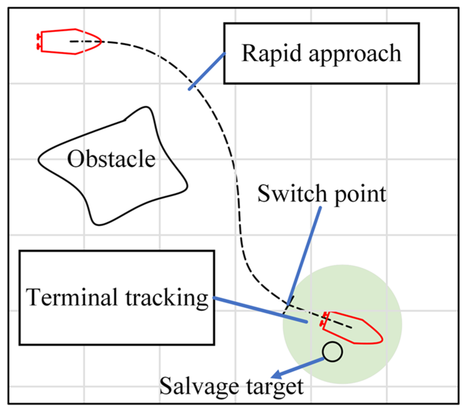
A surface salvage target tracking algorithm is proposed. The algorithm is divided into two phases, based on the distance between the salvage target and the USV: rapid approach and terminal tracking. The output of the salvage target tracking algorithm consists of the desired heading and the desired speed.

(2)

In the rapid approach phase, the model predictive line-of-sight guidance algorithm and path-following control algorithm are introduced. The PLOS guidance algorithm comprehensively considers a segment of the path information to optimally determine the desired heading, thereby improving the accuracy of curved path following. In the terminal tracking phase, a key point guidance algorithm-based method is proposed to track stationary or moving salvage targets. This method ensures that the distance between the salvage target and the USV remains within the salvage radius.

(3)

A PID-based heading and speed controller is developed to track the desired heading and speed. By adjusting the rotational speeds of the left and right propellers, the USV is driven to accomplish the tracking of the surface salvage target.

The remainder of this paper is organized as follows. In Section 2, the model of the salvage target tracking problem and the dynamic model of the TPNR USV are introduced. The methodology of the salvage target tracking system is described in Section 3. Moreover, the setting and results of numerical analysis are demonstrated in Section 4 and Section 5, respectively. Finally, the conclusions are shown in Section 6.

2. Control Objective Description

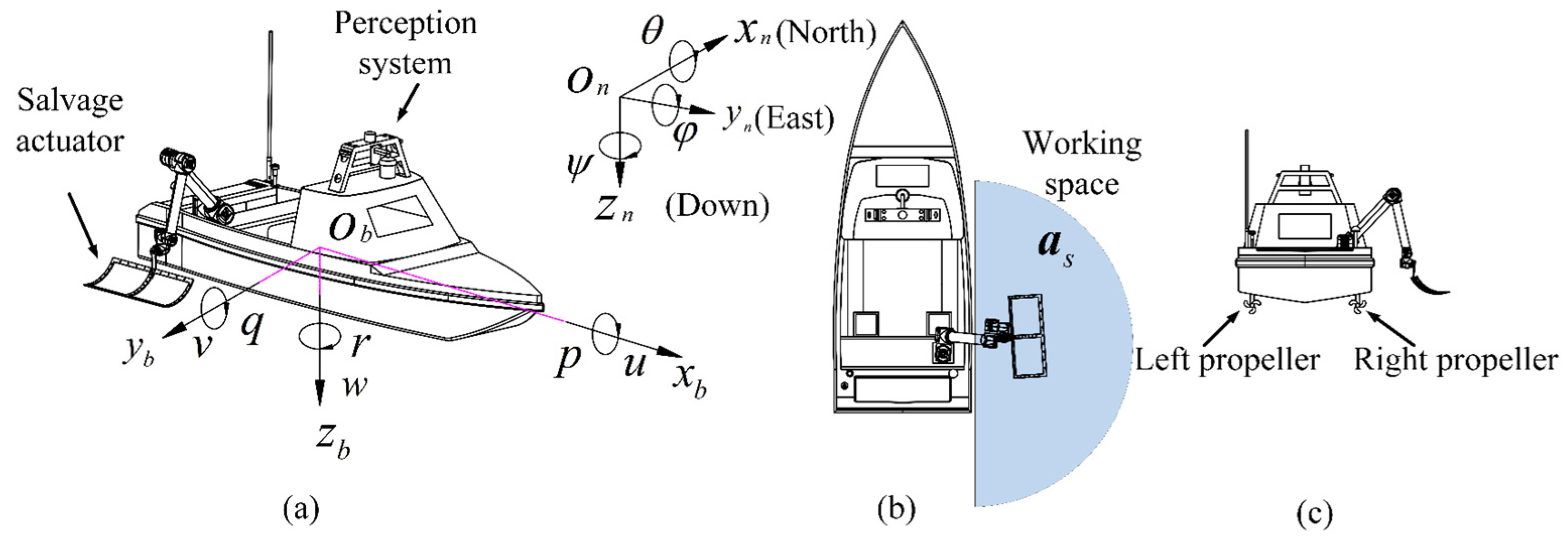
2.1. Configuration of Unmanned Surface Vehicle

Consider the scenario of a water area with shipwrecks or individuals overboard that necessitate salvage operations. A USV is used to execute the salvage mission. The USV is composed of a perception system, a salvage actuator, and a propulsion system, as shown in Figure 1. The perception system integrates a lidar module, a visual camera, and a real-time kinematic (RTK) positioning system to measure the orientation ${\psi }_t$, the distance $l_t$ of the salvage target relative to the USV, and the global position of the USV. Moreover, the salvage actuator is a six-degree-of-freedom serial manipulator integrated with an end-effector salvage net assembly. The manipulator is mounted on the starboard aft section of the USV, specifically designated for executing salvage operations. The propulsion system consists of left and right propellers symmetrically distributed along the centerline of the USV, without rudders. For the USV operating on the water surface, it is necessary to control its three degrees of freedom: surge, sway, and yaw. However, the two propellers only generate control forces in the surge and yaw directions, making the system underactuated due to its inability to control sway.

Furthermore, the north–east–down (NED) coordinate system $\left\{n\right\}=(x_n,y_n,z_n)$ is used as the global coordinate system, as shown in Figure 1a. The positive direction of the $y_n$ axis points to the east. The positive direction of the $x_n$ axis points to the north. The body-fixed coordinate system $\left\{b\right\}=(x_b,y_b,z_b)$ is used as the local coordinate system. The body-fixed coordinate system is attached to the hull of the USV. The origin of the body-fixed coordinate system is located at the center of gravity of the USV, with the positive $x_b$ oriented toward the bow and the positive $y_b$ directed toward the starboard side of the USV.

By utilizing the defined north–east–down and body-fixed coordinate system, the positions of the USV and the salvage target can be specified to facilitate the description of control objectives. The position of the origin of the body-fixed coordinate system in the global coordinate system is defined as $P_v=(x,y)\in {ℝ}^2$, where $x$ denotes the position in the eastward direction and $y$ represents the position in the northward direction. ${ℝ}^2$ represents the horizontal plane space. It is assumed that the orientation ${\psi }_t$ and distance $l_t$ of the salvage target are obtained with the assistance of the perception system.

Additionally, the position of the salvage target center $P_t=(x_t,y_t)\in {ℝ}^2$ can be calculated by $P_t=(x+l_t\cos {\psi }_t,y+l_t\sin {\psi }_t)$, where $x_t$ denotes the position of the salvage target in the eastward direction and $y_t$ represents the position of the salvage target in the northward direction. If the salvage target moves with the ocean current, the speed of the salvage target $u_t$ is equivalent to the ocean current speed. The projection of the working space of the salvage actuator onto the horizontal plane is defined as $a_s$; it is a semicircle.

According to the requirements of the docking position, the control objective can be formalized as

$$\underset{t\to \infty }{\lim }\left(x_t,y_t\right)\in a_s$$

(1)

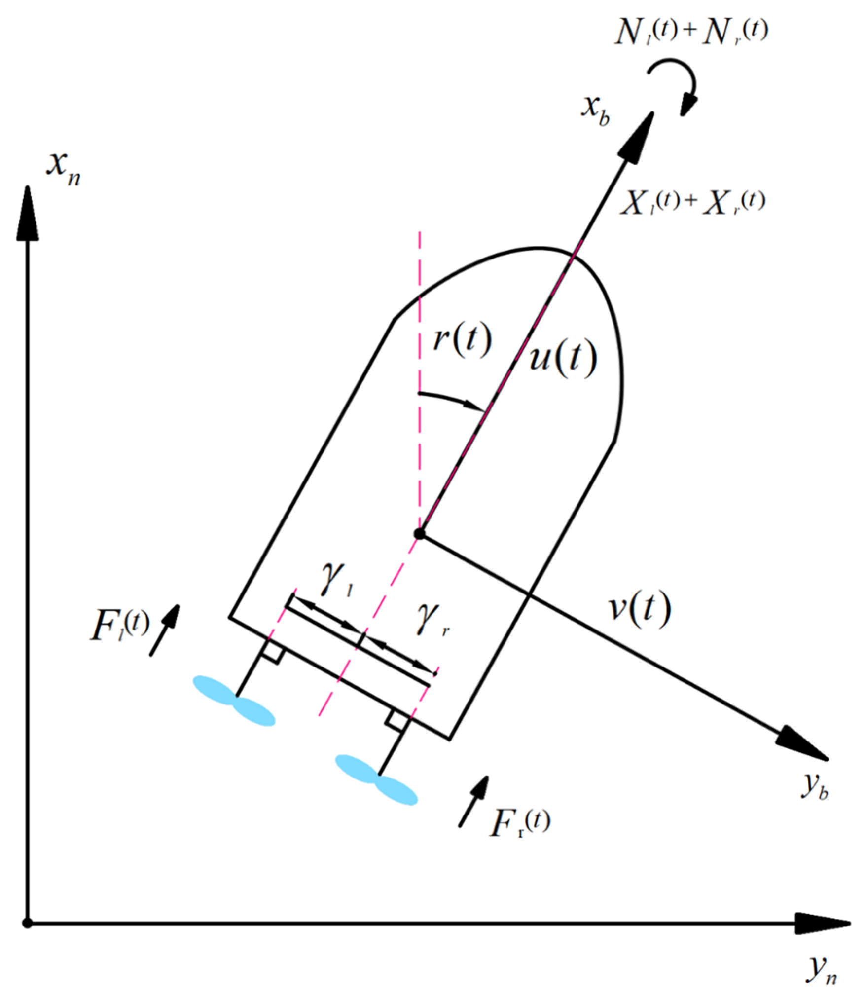
2.2. Mathematical Model of Twin-Propeller and Non-Rudder Unmanned Surface Vehicle

The kinematics model of the USV is obtained as

$$\left\{\begin{array}{l}\dot{x}=u\cos \psi -v\sin \psi \hfill \\ \dot{y}=u\sin \psi +v\cos \psi \hfill \\ \dot{\psi }=r\hfill \end{array}\right.,$$

(2)

by the transformation between the global coordinate system and the body-fixed coordinate system. The superscript dot denotes the derivative with respect to time. $u$, $v$, and $r$ denote the surge speed, sway speed, and yaw angular speed, respectively. Additionally, $\psi$ is the heading of the USV.

The following nonlinear three-degree-of-freedom dynamic model of an underactuated USV is established as

$$\left\{\begin{array}{l}\dot{u}={\displaystyle \frac{m_v}{m_u}}vr+{\displaystyle \frac{X_u}{m_u}}u+{\displaystyle \frac{{\tau }_u}{m_u}}\\ \dot{v}=-{\displaystyle \frac{m_u}{m_v}}ur-{\displaystyle \frac{Y_v}{m_v}}v+{\displaystyle \frac{{\tau }_v}{m_v}}\\ \dot{r}={\displaystyle \frac{m_u-m_v}{m_r}}ur-{\displaystyle \frac{N_r}{m_r}}r+{\displaystyle \frac{{\tau }_r}{m_r}}\end{array}\right.,$$

(3)

where $m_u=m-X_{\dot{u}}$, $m_v=m-Y_{\dot{v}}$, and $m_r=I_z-N_{\dot{r}}$. Here, $X_{\dot{u}}$, $Y_{\dot{v}}$, and $N_{\dot{r}}$ represent the added mass in the surge, sway, and yaw directions, respectively. $I_z$ refers to the moment of inertia of the USV mass about the $z_b$ axis. $X_u$, $Y_v$, and $N_r$ represent the hydrodynamic damping in the surge, sway, and yaw directions, respectively. ${\tau }_u$, ${\tau }_v$, and ${\tau }_r$ refer to the external forces on the USV in the surge, sway, and yaw directions, respectively.

For a USV equipped with only two propellers and no rudder, the propulsion provided by the propeller can be calculated as

$$\left\{\begin{array}{l}{X}_l(t)=(1-k_g)F_l(t)\\ Y_l(t)=0\\ N_l(t)=(1+k_h)d_l{F}_l(t)\end{array}\right.,$$

(4)

$$\left\{\begin{array}{l}{X}_r(t)=(1-k_g)F_r(t)\\ Y_r(t)=0\\ N_r(t)=(1+k_h)d_r{F}_r(t)\end{array}\right.,$$

(5)

where $F_l(t)$ and $F_r(t)$ denote the propulsion generated by the left and right propellers, respectively. The corresponding surge forces are denoted by $X_l(t)$ and $X_r(t)$, and the sway forces as $Y_l(t)$ and $Y_r(t)$. Additionally, the corresponding yaw moments are represented as $N_l(t)$ and $N_r(t)$, generated by the left and right propellers through propulsion deduction. $k_g$ is the propulsion deduction coefficient, which accounts for the reduction in effective thrust due to interaction between the hull and the propellers. $k_h$ denotes the coefficient that quantifies the contribution of differential propeller thrust to the yaw moment, reflecting the turning effect induced by varying the speed of the left and right propellers. $d_l$ and $d_r$ are the distances from the left propeller and the right propeller to the USV central axis, respectively. Because the position of the two propellers is symmetrical along the central axis of the hull, namely $d_l=d_r=d_0$, the propulsion model of the USV is as follows:

$$\left\{\begin{array}{l}{\tau }_u(t)=(1-k_g)(F_l(t)+F_r(t))\\ {\tau }_v(t)=0\\ {\tau }_r(t)=(1+k_h)d_0(F_l(t)-F_r(t))\end{array}\right.,$$

(6)

where ${\tau }_u(t)$, ${\tau }_v(t)$, and ${\tau }_r(t)$ are the forces in the surge, sway, and yaw directions, respectively. The force diagram of the TPNR USV is shown in Figure 2.

Substituting Equation (6) into Equation (3), the dynamic model of the TPNR USV is conducted as

$$\left\{\begin{array}{l}\dot{u}={\displaystyle \frac{m_v}{m_u}}vr+{\displaystyle \frac{X_u}{m_u}}u+{\displaystyle \frac{(1-g)(F_l(t)+F_r(t))}{m_u}}\\ \dot{v}=-{\displaystyle \frac{m_u}{m_v}}ur-{\displaystyle \frac{Y_v}{m_v}}v\\ \dot{r}={\displaystyle \frac{m_u-m_v}{m_r}}ur-{\displaystyle \frac{N_r}{m_r}}r+{\displaystyle \frac{(1+h)\gamma (F_l(t)-F_r(t))}{m_r}}\end{array}\right..$$

(7)

In the subsequent Section 3, the control algorithm will be presented to achieve the control objective proposed in this section. The dynamic model of the twin-propeller and non-rudder USV established in this section will be utilized in the numerical analysis conducted in Section 4.

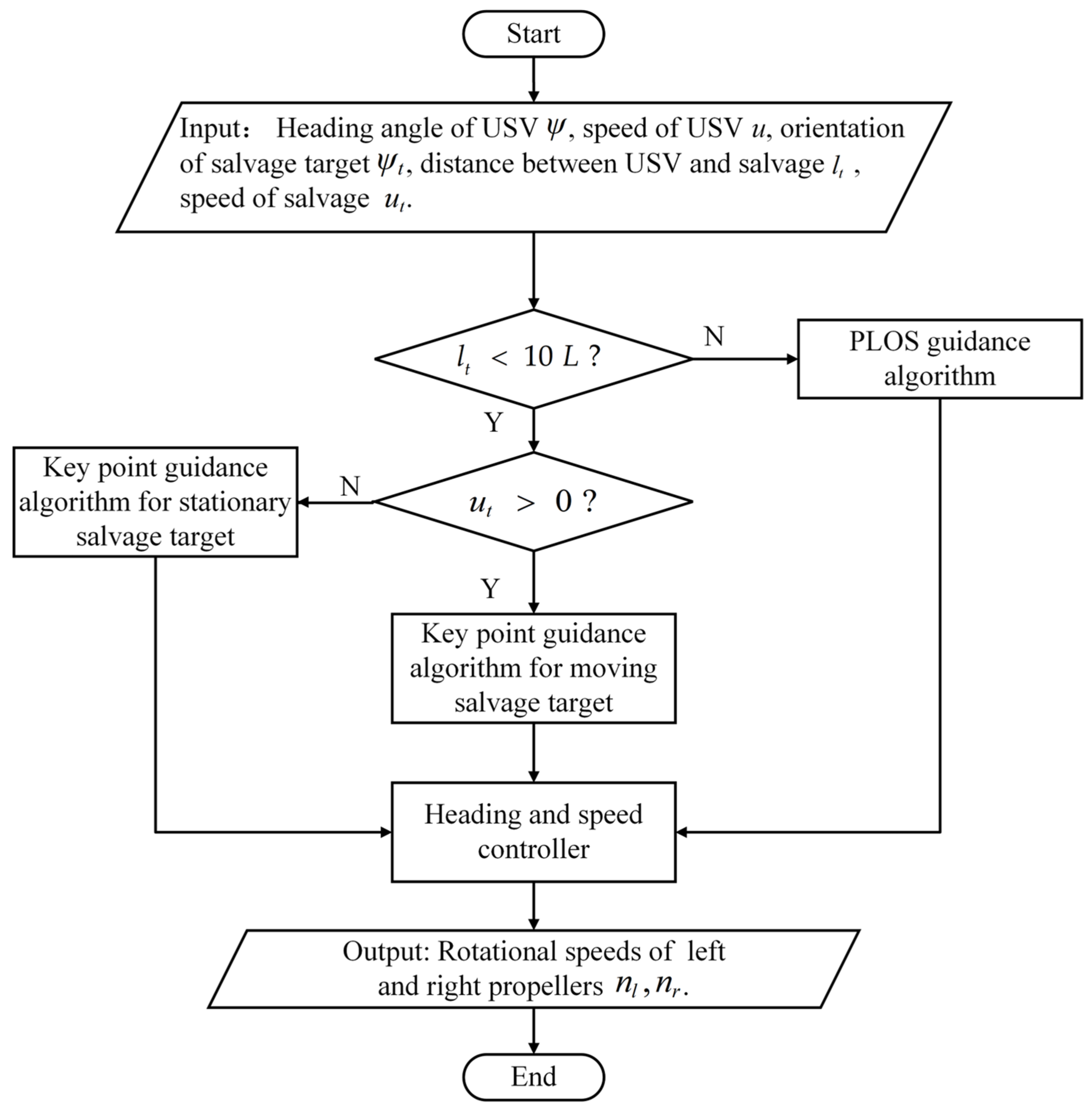
3. Structure of Salvage Target Tracking Algorithm

In this section, the salvage target tracking algorithm is designed based on the control objective outlined in Section 2. The algorithm consists of the rapid approach phase and the terminal tracking phase, which proceed according to the distance between the USV and the salvage target, as shown in Figure 3. The algorithm operates in the rapid approach phase when the distance between the USV and the target exceeds a defined threshold, and switches to terminal tracking when the distance falls below this threshold. The threshold is set to 10 times the length of the USV $L$, ensuring sufficient adjustment distance for subsequent tracking operations. Additionally, the rapid approach phase and terminal tracking phase are implemented through a heading and speed controller.

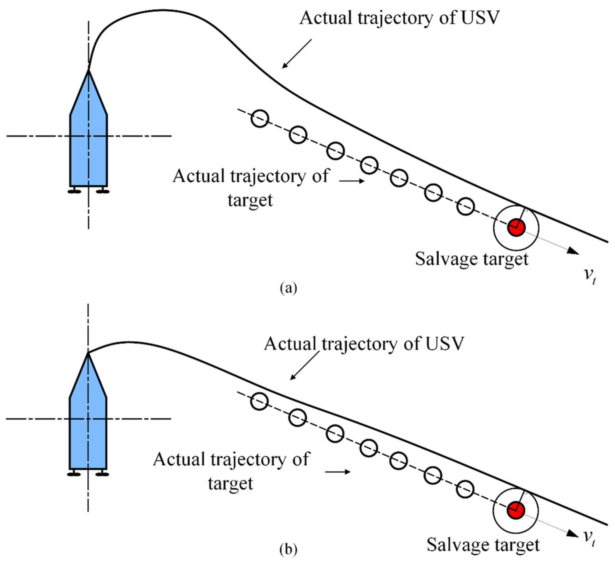
3.1. Rapid Approach Phase

For the rapid approach phase, the USV sails towards the salvage target at maximum speed along the reference path. The model predictive line-of-sight guidance algorithm is proposed to enable the USV to follow the reference path.

The PLOS guidance algorithm consists of cross-tracking error calculation, path segmentation, and desired-heading calculation. The calculation of the cross-tracking error defines the deviation between the position of the USV and the desired position; furthermore, it will be utilized in the calculation of the desired heading. Path segmentation divides the pre-planned path into straight-line segments and curved segments based on the curvature of the path and the yaw rate of the USV. The desired heading is computed separately for straight and curved path segments. In the path following, a non-zero drift angle is introduced to reduce the tracking error caused by the steering hysteresis effect, enabling the USV to initiate turning maneuvers in advance. The drift angle is determined based on the model prediction.

In order to calculate the cross-tracking error, it is necessary to identify the closest point to the USV on the pre-planned path. The reference path $\Gamma$, consisting of a series of waypoints, is a non-closed path, as shown in Figure 4. $\left(x_{\mathrm{c}}(\omega ),y_{\mathrm{c}}(\omega )\right)$ is the closest point on the desired path to the origin of the body-fixed coordinate; it is determined by

$$\left(x_c,y_c,\omega \right)=\arg \underset{\left(x_i,y_i,\omega \right)\in \Gamma }{\min }\parallel \left(x_i^p,y_i^p\right)-\left(x,y\right)\parallel ,$$

(8)

where $x_c$ and $y_c$ represent the eastward and northward positions of the closet point in the north–east–down coordinate, respectively. $x_i^p$ and $y_i^p$ represent the eastward and northward positions of the i-th path point in the north–east–down coordinate, respectively. $\omega$ is a positive path variable.

The cross-tracking error $y_e$ is calculated by

$$y_e=-(x-x_c(\omega ))\sin ({\gamma }_c)+(y-y_c(\omega ))\cos ({\gamma }_c),$$

(9)

where ${\gamma }_c$ denotes the angle between the north axis $x_n$ and the tangent line at the point $\left(x_{\mathrm{c}}(\omega ),y_{\mathrm{c}}(\omega )\right)$ on the desired path $\Gamma$, and it is expressed as ${\gamma }_c=\mathrm{atan}2(y_c^{\prime }(\omega ),x_c^{\prime }(\omega ))$, where $x_c^{\prime }=\partial x_{\mathrm{c}}(\omega )/\partial \omega$, $y_c^{\prime }(\omega )=\partial y_{\mathrm{c}}(\omega )/\partial \omega$.

A judgment factor $\kappa$ is utilized to segment the path, which is calculated by

$$\kappa ={\displaystyle \frac{u\partial {\gamma }_c}{r_{\max }\partial x}},$$

(10)

where $\partial {\gamma }_c/\partial x$ is the derivative of the tangent angle of the path with respect to the eastward coordinate. $r_{\max }$ is the maximum turning speed of the USV.

The path is defined as a straight line when $\kappa <1.05$. The guidance algorithm is the same as LOS guidance algorithm. The desired heading is calculated by

$${\psi }_d={\gamma }_c-\arctan \left({\displaystyle \frac{y_e}{\mathsf{\Delta }}}\right),$$

(11)

where $\Delta$ is the look-ahead distance; it is usually set as 1.5 to 2 times the length of the USV. When the control subsystem realizes $\forall \epsilon >0$, ${\lim }_{t\to \infty }({\psi }_{\mathrm{d}}-\psi )\le \epsilon$, the USV can converge to the pre-planned path.

The path is defined as a curved path when $\kappa >1.05$. The steering hysteresis effect caused by the curvature of the path is non-negligible. Because in Equation (11), the desired heading is proportional to the cross-tracking error $y_e$, when $y_e\to 0$, then ${\psi }_d\to {\gamma }_c$. It only considers the information of the projection point $\left(x_{\mathrm{c}}(\omega ),y_{\mathrm{c}}(\omega )\right)$ at each sampling time. When the direction of the path ahead continuously changes, the USV will move off the path, causing cross-tracking error before being guided to the tracking path, as shown in Figure 5a.

The PLOS guidance algorithm introduces the drift angle on the basis of the LOS guidance algorithm to compensate for the cross-tracking error caused by the steering hysteresis effect, as shown in Figure 5b. The desired heading is calculated by

$${\psi }_d={\gamma }_c-\arctan \left({\displaystyle \frac{1}{\mathsf{\Delta }}}{y}_e\right)+\widehat{\beta }{\displaystyle \frac{\left|y_c^{″}\right|}{y_c^{″}}},$$

(12)

where $\widehat{\beta }$ is the drift angle, and $y_c^{″}$ is the second derivative of the path, calculated by

$$y_c^{″}={\displaystyle \frac{y_c^{″}(\omega )x_c^{\prime }(\omega )-x_c^{″}(\omega )y_c^{\prime }(\omega )}{{x_c^{\prime }}^3(\omega )}},$$

(13)

and $y_c^{″}(\omega )=\partial y_c^{\prime }(\omega )/\partial \omega$, $x_c^{″}(\omega )=\partial x_c^{\prime }(\omega )/\partial \omega$.

In order to compute the value of $\widehat{\beta }$ that minimizes the cross-tracking error, the prediction model of the path-following system is established as

$${\dot{\mathit{x}}}_N(t)=f_N({\mathit{x}}_N(t),u(t)),$$

(14)

where $f_N$ is the state-space equation composed of the state variable $x_N(t)$ and the input $u(t)$; it can be calculated by

$$f_N({\mathit{x}}_N(t),u(t))=\left[\begin{array}{c}{x}_{N6}\\ \cos (x_{N1})x_{N4}-\sin (x_{N1})x_{N5}\\ \sin (x_{N1})x_{N4}+\cos (x_{N1})x_{N5}\\ {\displaystyle \frac{{\tau }_1}{m-X_{\dot{u}}}}\\ -{\displaystyle \frac{m_u}{m_v}}{x}_{N4}{x}_{N6}-{\displaystyle \frac{Y_v}{m_v}}{x}_{N5}+{\displaystyle \frac{{\tau }_v}{m_v}}\\ {\displaystyle \frac{m_u-m_v}{m_r}}{x}_{N4}{x}_{N6}-{\displaystyle \frac{N_r}{m_r}}{x}_{N6}+{\displaystyle \frac{{\tau }_r}{m_r}}\end{array}\right],$$

(15)

where ${\mathit{x}}_N(t)={\left[\begin{array}{cccccc}{x}_{N1}& x_{N2}& x_{N3}& x_{N4}& x_{N5}& x_{N6}\end{array}\right]}^T={\left[\begin{array}{cccccc}\psi & x& y& u& v& r\end{array}\right]}^T$. The input of the system is $u(t)={\left[\begin{array}{ccc}{\tau }_1& {\tau }_2& {\tau }_3\end{array}\right]}^T$. The control force is computed based on the desired heading and the actual heading.

Continuous state-space equations are discretized into

$$x_N(k+1)=x_N(k)+f_N(x_N(k),u(k))t_{step},$$

(16)

where $k$ represents the computation step number and $t_{step}$ is the predicted step size.

The optimization goal is to minimize the cross-tracking error. The optimization problem is constructed to determine the drift angle as follows:

$$\widehat{\beta }=\underset{\beta \in \left[{\beta }_{\min },{\beta }_{\max }\right]}{\arg \min }\left\{{\displaystyle \sum }_{i=1}^{N_p}{y}_c\left({\omega }_i\right)-\left[\begin{array}{c}0 0 1 0 0 0\end{array}\right]·x_N\left(k+i\right)\right\},$$

(17)

where $N_P$ is the number of predicted steps, ${\beta }_{\min }=-15°$, and ${\beta }_{\max }=15°$.

Through the PLOS guidance algorithm, the information of multiple path points can be considered for guidance. The calculated drift angle $\widehat{\beta }$ will enable the USV to initiate a turning maneuver in advance, thereby compensating for the cross-tracking error.

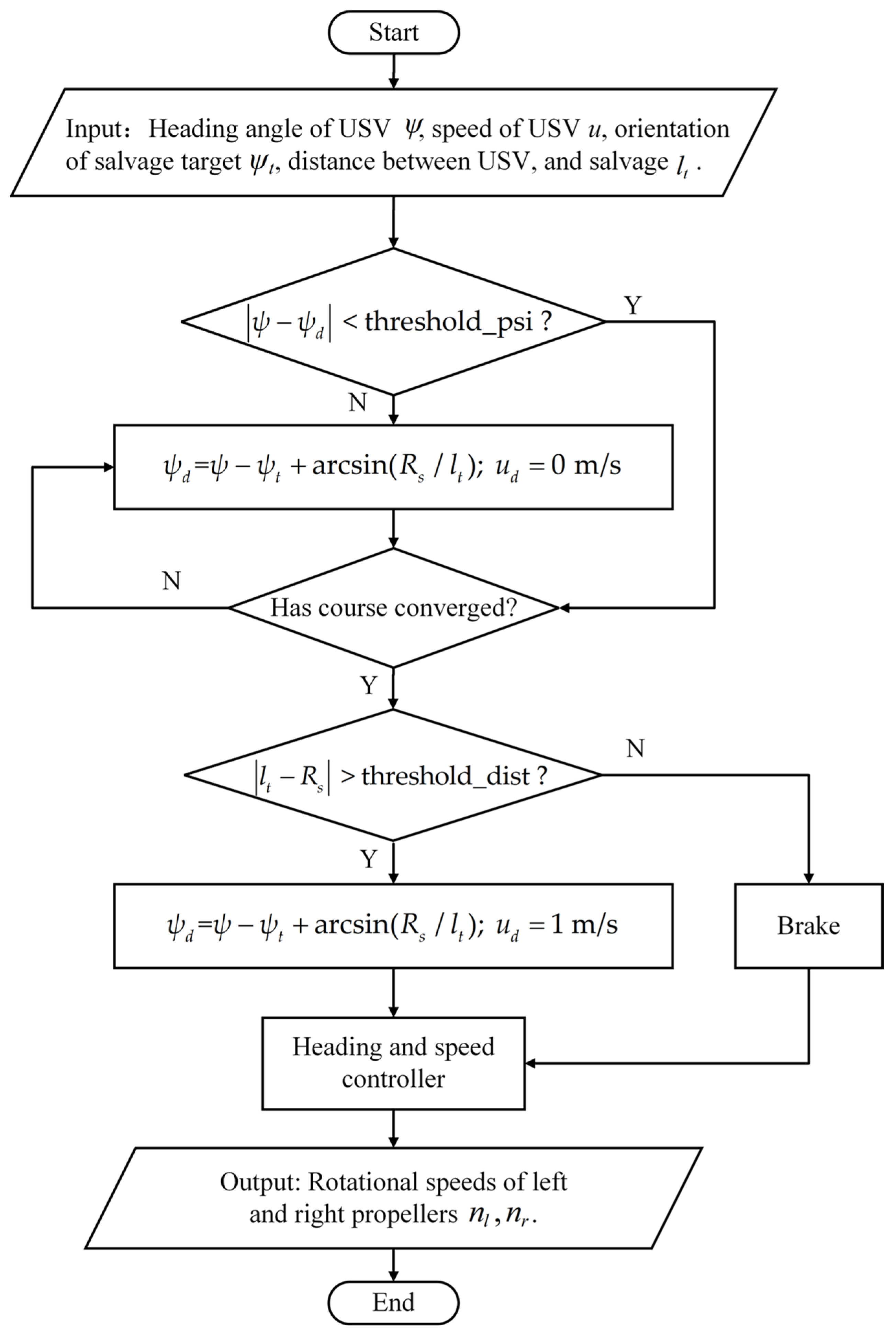
3.2. Terminal Tracking Phase

In the terminal tracking phase, a key point guidance algorithm is proposed for tracking the salvage target, comprising two modules: stationary salvage target tracking and moving salvage target tracking.

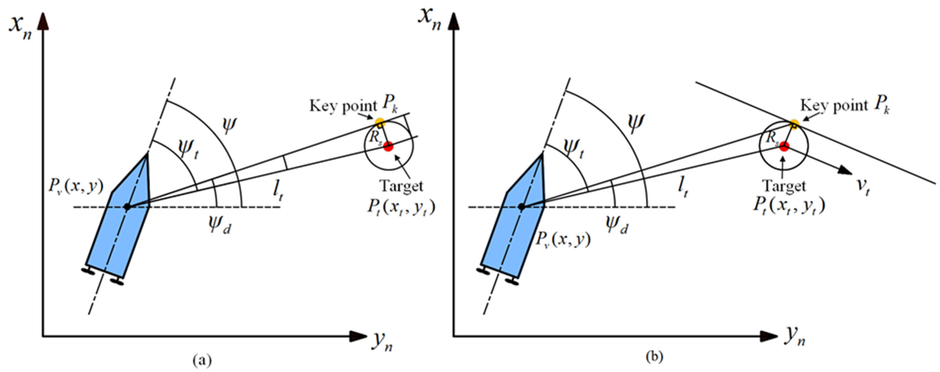
3.2.1. Key Point Guidance Algorithm for Stationary Salvage Target

The key point is selected to calculate the desired heading of the USV for tracking the stationary salvage target. To ensure contact between the salvage actuator and the target, the distance between the USV and the salvage target should be less than the maximum working radius of the salvage actuator. Therefore, an auxiliary circle is constructed with $P_t(x_t,y_t)$ as the center, and its radius $R_s$ equal to 0.8 times the radius of the working space of the salvage actuator. Additionally, the key point is positioned on the auxiliary circle to ensure that the docking position of the USV remains within the reachable workspace of the salvage actuator.

In order to describe the position of the key point, $\overrightarrow{AB}$ is defined as a vector that points from point $A$ to point $B$ in the north–east–down coordinate system $O_n-x_n{y}_n{z}_n$. Moreover, $\angle \overrightarrow{AB}$ represents the angle formed between the vector $\overrightarrow{AB}$ with the axis of $x_n$, and $‖\overrightarrow{AB}‖$ represents the Euclidean norm of the vector $\overrightarrow{AB}$.

In order to obtain the position of the key point, a tangent line should be drawn to the auxiliary circle which passes through the origin of the body-fixed coordinate system $P_v(x,y)$. The tangent point is selected as the key point. In the geometric context, it can be determined that there are two tangent lines satisfying the given geometric conditions. Subsequently, the selection of the tangent line is contingent upon the specific installation location of the salvage actuator. The salvage actuator is installed on the starboard side of the USV. The tangent line is obtained by rotating vector $\overrightarrow{P_v{P}_t}$ in a counter-clockwise direction about the point $P_v$, as shown in Figure 6a. Therefore, the desired heading can be calculated by

$${\psi }_d=\angle {\overrightarrow{P_{v}P}}_k=\psi -{\psi }_t+\arcsin {\displaystyle \frac{R_s}{l_t}}.$$

(18)

In order to track the stationary salvage target, the desired speed of the USV needs to be planned. The desired speed of the USV is planned in three stages. Initially, before the actual heading converges to the desired heading, the speed is set to zero. Subsequently, when the actual heading of the USV converges to the desired heading and remains stable, the desired speed of the USV is set to 1 m/s. Finally, when $\left|l_t-R_s\right|\le 0.1b$, where $b$ represents the width of the USV, the left and right propellers operate at full speed in reverse until the speed drops to zero. At this moment, the USV has entered the working space of the salvage actuator. The specific implementation process of the key point guidance algorithm for a stationary salvage target is shown in Figure 7.

3.2.2. Key Point Guidance Algorithm for Moving Salvage Target

When tracking the moving salvage target, the trajectory of the USV must remain parallel to the trajectory of the salvage target, with the USV positioned on the right side of the trajectory of the salvage target. Therefore, the intersection point where the speed vector of the target is rotated counter-clockwise by $\pi /2$ rad and intersects with the auxiliary circle is selected as the key point, as shown in Figure 6b. The key point is selected to calculate the desired heading of the USV; the desired heading can be calculated by

$${\psi }_d=\angle \overrightarrow{P_v{P}_k}=\angle (\overrightarrow{P_v{P}_t}+R(\theta ){\displaystyle \frac{‖u_t‖}{u_t}}{R}_S),$$

(19)

where $R(\theta )$ represents the rotation matrix, and $\theta$ represents the rotation angle, which is set as $\pi /2$ rad. Under the influence of the rotation matrix, the vector $u_t$ is rotated counter-clockwise by $\pi /2$ rad around the center of the salvage target.

The desired speed of the USV is determined by the distance between the USV and the salvage target. With the distance error between the USV and the salvage target defined as $\tilde{d}=l_t-R_s$, the desired speed of the USV is given by

$$u_d=k_{barrier}(k_p^t\tilde{d}+k_i^t{\displaystyle \int \tilde{d}}),$$

(20)

where $k_p^t$ and $k_i^t$ are the proportional and integral tracking control parameters, respectively. $k_{barrier}$ is the speed-limiting factor, calculated by

$$k_{barrier}=-\left|\tanh (\tilde{\psi })+1\right|,$$

(21)

where $\tilde{\psi }$ is the heading error that calculated by $\tilde{\psi }=\psi -{\psi }_d$.

When the USV has not converged to the desired heading, the speed-limiting factor approaches zero, resulting in a desired speed close to zero. As a result, the turning radius of the USV is decreased, and the potential for overshoot is reduced. Consider a scenario in which the speed vector of the salvage target points towards the fourth quadrant of the body-fixed coordinate system. The turning radius of the USV depends on its speed; excessive speed may result in an overshoot, as illustrated in Figure 8a. A function graph of the speed-limiting factor is shown in Figure 9. When the heading error is large, the speed-limiting factor can make the speed of the USV approach zero, causing the trajectory shown in Figure 8b.

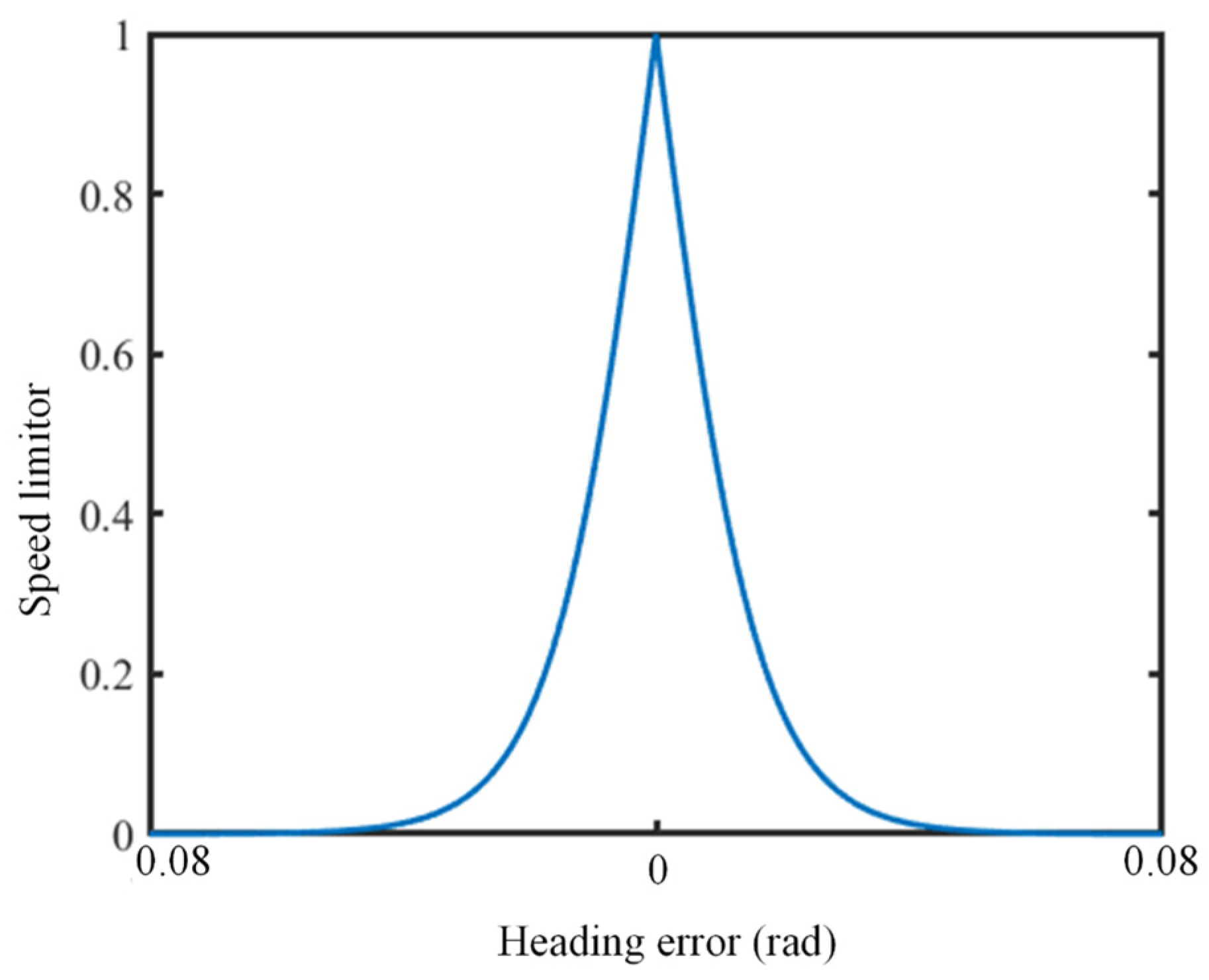
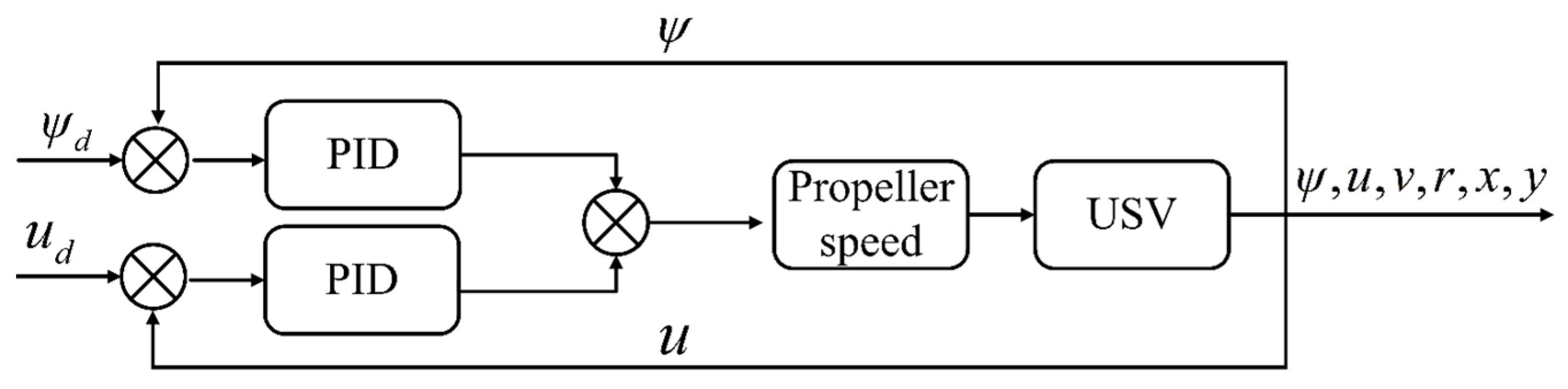
3.3. Heading and Speed Controller

3.3.1. Design of Heading and Speed Controller

In this subsection, a heading and speed controller is proposed to track the desired heading and desired speed calculated by the PLOS guidance algorithm in the RA phase and the key point guidance algorithm in the TT phase. The controller is implemented based on the PID, and a schematic diagram of the controller is shown in Figure 10.

First, the speed error $\tilde{u}$ and the heading error $\tilde{\psi }$ are defined by

$$\left\{\begin{array}{l}\tilde{u}=u_d-u\\ \tilde{\psi }={\psi }_d-\psi \end{array}\right.,$$

(22)

The subscript d represents the desired value calculated by the PLOS guidance algorithm in the RA phase and the key point guidance algorithm in the TT phase.

The virtual control variables of the speed $n_v$ and the heading $n_h$ are calculated by

$$\left\{\begin{array}{l}{n}_v=k_{vp}\tilde{u}+k_{vi}\int \tilde{u}+k_{vd}{\displaystyle \frac{d\tilde{u}}{dt}}\\ n_h=k_{hp}\tilde{\psi }+k_{hi}\int \tilde{\psi }+k_{hd}{\displaystyle \frac{d\tilde{\psi }}{dt}}\end{array}\right.,$$

(23)

where $k_{vp}$, $k_{vi}$, $k_{vd}$, $k_{hp}$, $k_{hi}$, and $k_{hd}$ are the parameters of the heading and speed controller.

The desired heading is adjusted by altering the difference in rotational speed between the left and right propellers. Meanwhile, to ensure a constant cruising speed, the sum of the rotational speeds of the left and right propellers should remain invariant. The rotational speeds of the left and right propellers are calculated by

$$\left\{\begin{array}{l}{n}_l={\displaystyle \frac{n_v}{2}}+n_h\\ n_r={\displaystyle \frac{n_v}{2}}-n_h\end{array}\right.,$$

(24)

where $n_l$ is the speed of the left propeller, $n_r$ is the speed of the right propeller, and $n_v$ and $n_h$ are the control variables for speed and heading, respectively.

3.3.2. Controller Parameter Tuning

In this subsection, the parameters of the proposed heading and speed controller are tuned using the Bayesian optimization method to achieve optimal performance.

The parameter vector of the heading and speed controller is defined as

$${\theta }_c={[\begin{array}{llllll}{k}_{vp}& k_{vi}& k_{vd}& k_{hp}& k_{hi}& k_{hd}\end{array}]}^{\mathrm{T}}\in {\Xi }_c\subset {ℝ}^6,$$

(25)

where ${\Xi }_c$ is the parameter space of the heading and speed controller.

The objective function of the Bayesian optimizer is defined as

$$J_c={\displaystyle {\int }_{T_c}^{T_c+5}{w}_1(\left|\tilde{u}\right|)}+w_2(\left|\tilde{\psi }\right|)dt+w_3{\tau }_c^u+w_4{\tau }_c^h,$$

(26)

where ${\tau }_c^u$ is the rise time of the speed; ${\tau }_c^h$ is the rise time of the heading; $w_1$, $w_2$, $w_3$, and $w_4$ are the evaluation weights for the heading and speed performance; and $T_c$ is the time at which both the heading and speed controlled by the controller first reach their desired values.

The purpose of Bayesian optimization is to search within the parameter space of the heading and speed controller for the parameter vector that minimizes the objective function:

$${\theta }_c^{\ast }=\arg \underset{{\theta }_c\in {\Xi }_c}{\min }{J}_c({\theta }_c).$$

(27)

Bayesian optimization constructs a probabilistic surrogate model of the objective function using a Gaussian process:

$$J(\theta )\sim GP(m(\theta ),k(\theta ,{\theta }^{\prime })),$$

(28)

where $m(\theta )$ is the mean function, representing the predicted mean at each point, which is typically set to zero in the absence of prior knowledge. $k(\theta ,{\theta }^{\prime })$ is the kernel function, which defines the covariance structure between different parameter points; it is defined as

$$k(\theta ,{\theta }^{\prime })={\sigma }_f^2\exp \left(-{\displaystyle \frac{\left|\right|\theta -{\theta }^{\prime }|{|}^2}{{2l_k}^2}}\right),$$

(29)

where ${\sigma }_f^2$ is the maximum value of the kernel function, and $l_k$ denotes the characteristic length scale of the kernel.

In Bayesian optimization, an acquisition function is a utility that is used to pick the next point in the parameter space to be explored. In this paper, the Expected Improvement (EI) is chosen as the acquisition function:

$${\alpha }_{\mathrm{EI}}(\mathit{\theta })=(J_{\min }-\mu (\mathit{\theta }))\Phi (Z)+\sigma (\mathit{\theta })\varphi (Z),$$

(30)

where $\Phi (Z)$ and $\varphi (Z)$ are the cumulative distribution function (CDF) and the probability density function (PDF) of the standard normal distribution, respectively. $Z$ represents the normalized improvement, which is given by

$$Z={\displaystyle \frac{J_{\min }-\mu (\mathit{\theta })}{\sigma (\mathit{\theta })}}.$$

(31)

Based on the acquisition function, the next set of controller parameters is determined by

$${\theta }_{k+1}=\arg \underset{\mathit{\theta }\in \Xi }{\max }\alpha (\mathit{\theta }).$$

(32)

Through iterative optimization, the parameter vector of the heading and speed controller that maximizes the acquisition function is repeatedly selected until the objective function converges or the maximum number of iterations is reached. The controller parameter vector obtained at this point is regarded as the optimal solution.

3.4. Section Summary

In summary, the STT algorithm is divided into two phases based on the distance between the USV and the salvage target; specifically, whether the distance between the USV and the salvage target is greater or less than 10 times the length of the USV. A key point guidance algorithm is proposed to calculate the desired heading and desired speed. The corresponding key point is selected according to the speed of the salvage target. To facilitate understanding of the tracking algorithm, the pseudo-code of the entire algorithm is presented in Figure 11.

4. Simulation Analysis

4.1. Setting of Numerical Analysis

In this section, the effectiveness of the proposed salvage target tracking algorithm will be verified by numerical analysis methods, with a focus on the effectiveness of the proposed heading and speed controller, the performance of the PLOS guidance algorithm, and the effectiveness of the key point guidance algorithm.

Two simulation scenarios were designed to verify whether the proposed heading and speed controller would be capable of driving the USV to track the desired heading and the desired speed. In the first scenario, the USV is required to track a time-varying heading at a constant speed. The desired speed of the USV is set as $u_d=1$ m/s, and the desired heading of the USV is set as $\sin (0.01t)$. In the second scenario, the USV is required to track the time-varying heading while maintaining a speed of zero. The desired speed of the USV is set as $u_d=0$ m/s, and the desired heading of the USV is also set as $\sin (0.01t)$. The design parameters for the heading and speed controller are configured as detailed in

Table 1. Design parameters of salvage target tracking control algorithm.

Phase of Algorithm	Parameter Name	Parameter Setting
Rapid approach phase	Look-ahead distance, $\Delta$	13.00 m
	Sampling period of discrete system, $t_{\mathrm{step}}$	0.10 s
	Maximum speed of USV, $u_{\max }$	5.00 m/s
Terminal tracking phase	Radius of auxiliary circle, $R_s$	5.00 m
	Allowable error of heading controller, threshold_psi	0.05 rad
Heading and speed controller	Speed proportional parameter, $k_{vp}$	9.00
	Speed integral parameter, $k_{vi}$	0.08
	Speed differential parameter, $k_{vd}$	0.70
	Heading proportional parameter, $k_{hp}$	5.00
	Heading integral parameter, $k_{hi}$	0.01
	Heading differential parameter, $k_{hd}$	1.00

.

Additionally, two sets of path-following simulations were conducted to verify the performance of the PLOS guidance algorithm by comparing it with the LOS guidance algorithm, integral line-of-sight (ILOS) guidance algorithm, and adaptive error constraint line-of-sight (AECLOS) guidance algorithm. In the first set of simulations, the path was obtained by performing cubic polynomial interpolation through the waypoints (0, 200), (400, 100), (800, 400), and (1300, 300). The initial position of the USV was set at (0, 100), and the initial speed of the USV was set as 0 m/s. The initial heading of the USV was set to −$\pi /4$ rad. In the second set of simulations, the path was a Dubins path, consisting of a straight line and an arc. The initial position of the USV was set at (−100, 300), and the initial speed of the USV was set as 0 m/s. The initial heading of the USV was set to 0 rad. In both simulations, the desired speed of the USV was set to the maximum speed recommended in the ISO 11592-1-2016 standard [33]. The parameters of the STT algorithm are shown in Table 1.

Moreover, the verification of the key point guidance algorithm was carried out by testing under two scenarios. In the first scenario, the position of the USV is set at the point (0, 0), and the position of the salvage target is set at (41, 43). The salvage target remains stationary. In the second scenario, the origin of the body-fixed coordinate is set at (0, 0), and the initial heading is $\pi /2$ rad. The initial position of the salvage target is set at (20, 0). The salvage target moves at a speed of 0.50 m/s in the east direction, with the ocean current. The parameters of the key point guidance algorithm are shown in Table 1.

The hydrodynamic parameters of the USV used in the simulation were $m_u=35.800$, $m_v=47.049$, $m_r=2.676$, $X_u=-0.422$, $N_r=-2.220$, and $Y_v=-1.600$. The structural parameters of the USV are shown in

Table 2. Main parameters of scaled-down USV.

Parameter Name	Value
Length of USV, $L$	6.00 m
Distance between left and right propellers, $2\gamma$	1.00 m
Width of USV, b	1.50 m
Propulsion deduction coefficient, $t_p$	0.40
Maximum rotational speed of left and right propellers, $n_{\max }$	15.00 r/s
Maximum angular acceleration of left and right propellers, ${\dot{n}}_{\max }$	5.00 r/s2
Diameter of left and right propellers, $D_P$	0.10 m
Advance coefficient of left and right propellers, $K_T$	0.32
Coefficient of left and right propellers influencing on turning moment, $b_p$	0.30

.

In the simulation, the propulsion provided by the propeller $F_p$ is calculated by

$$F_p=\rho \left|n\right|n{D}_P^4{K}_T,$$

(33)

where $\rho$ is the density of the seawater, taken as $1\times {10}^3{\mathrm{kg}/\mathrm{m}}^3$; $n$ is the rotational speed of the propeller; $D_P$ is the diameter of the propeller; and $K_T$ is the advance coefficient of the propeller.

Furthermore, constraints on the maximum rotational speed and maximum angular acceleration are employed in the simulation to improve practicality. The restriction rule of the maximum rotational speed is calculated as

$$n=\left\{\begin{array}{ll}{n}_{\max }& n>n_{\max }\\ n& n<n_{\max }\end{array}\right.,$$

(34)

where $n_{\max }$ is the maximum rotational speed of the propeller.

Additionally, the restriction rule of maximum angular acceleration is calculated as

$$n^{k+1}=\left\{\begin{array}{ll}{n}^k+t_{\mathrm{step}}{\dot{n}}_{\max }\hfill & \dot{n}>{\dot{n}}_{\max }\\ n^k+t_{\mathrm{step}}\dot{n}\hfill & \dot{n}<{\dot{n}}_{\max }\end{array}\right.,$$

(35)

where ${\dot{n}}_{\max }$ is the maximum angular acceleration of the propeller; $n^k$ is the rotational speed of the propeller at step k; and $n^{k+1}$ is the rotational speed of the propeller at step k + 1.

The simulation was performed with a time step of 0.1 s. The hardware configuration of the computer used for the computation included an Intel Core i7-8700 CPU and an NVIDIA GeForce RTX 3060 Ti GPU. The algorithm’s memory usage was 3.13 MB. During runtime, the CPU utilization remained below 30%. The average execution time per control cycle was 8.5 ms.

The effectiveness of the proposed heading and speed controller was evaluated by analyzing the heading error and the speed error of the USV. When tracking the time-varying heading, if the heading error and speed error were bounded, the heading and speed controller was considered to be effective.

The performance of the proposed PLOS guidance algorithm was evaluated by comparing its path-following accuracy with that of LOS guidance algorithm, ILOS guidance algorithm, and AECLOS guidance algorithm. The path-following accuracy of the guidance algorithms was quantified using the cross-tracking error. The average of the cross-tracking error was calculated to measure the overall accuracy of the guidance algorithms. The standard deviation was calculated to evaluate the degree of dispersion of the error generated by the guidance algorithms. The root mean square error of the cross-tracking error was calculated to evaluate the deviation between the actual position and the expected position of the USV.

The distance between the USV and the salvage target and the orientation of the salvage target were used to evaluate the key point guidance algorithm. It was considered that if the distance between the USV and the target was less than the working radius of the salvage actuator, the key point guidance algorithm could be considered an effective guidance algorithm.

4.2. Results of Numerical Analysis

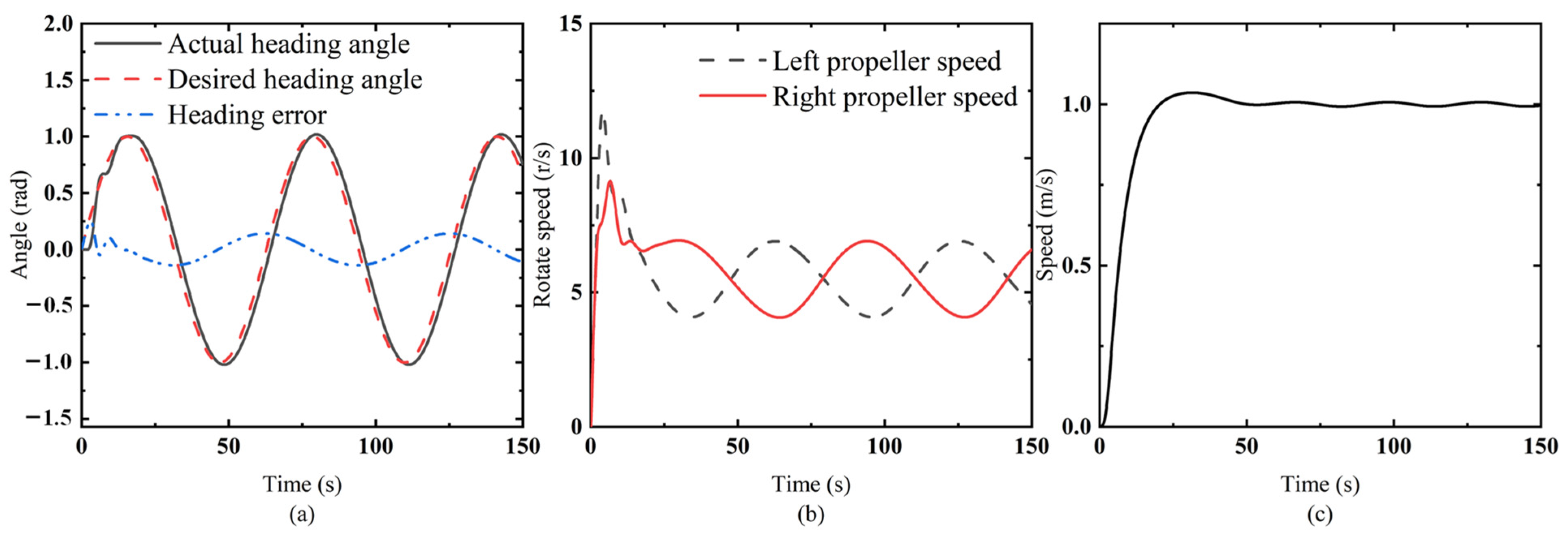
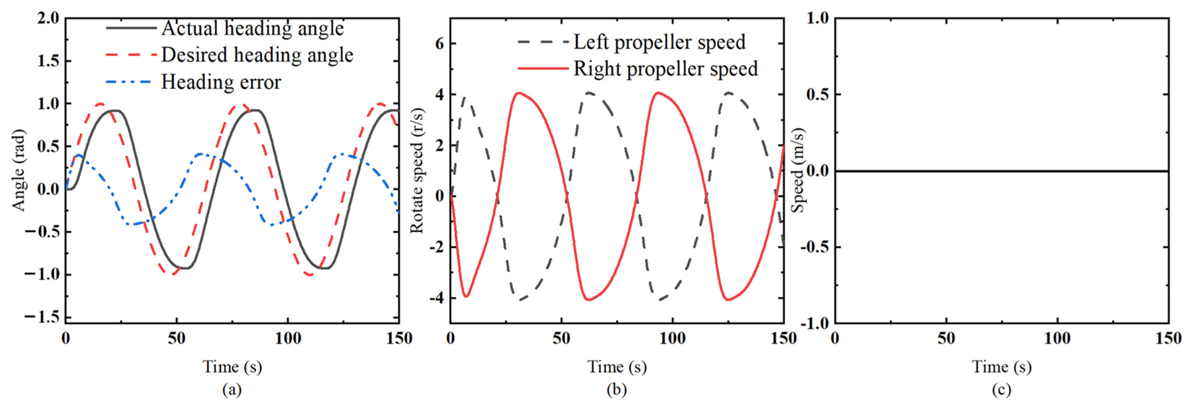
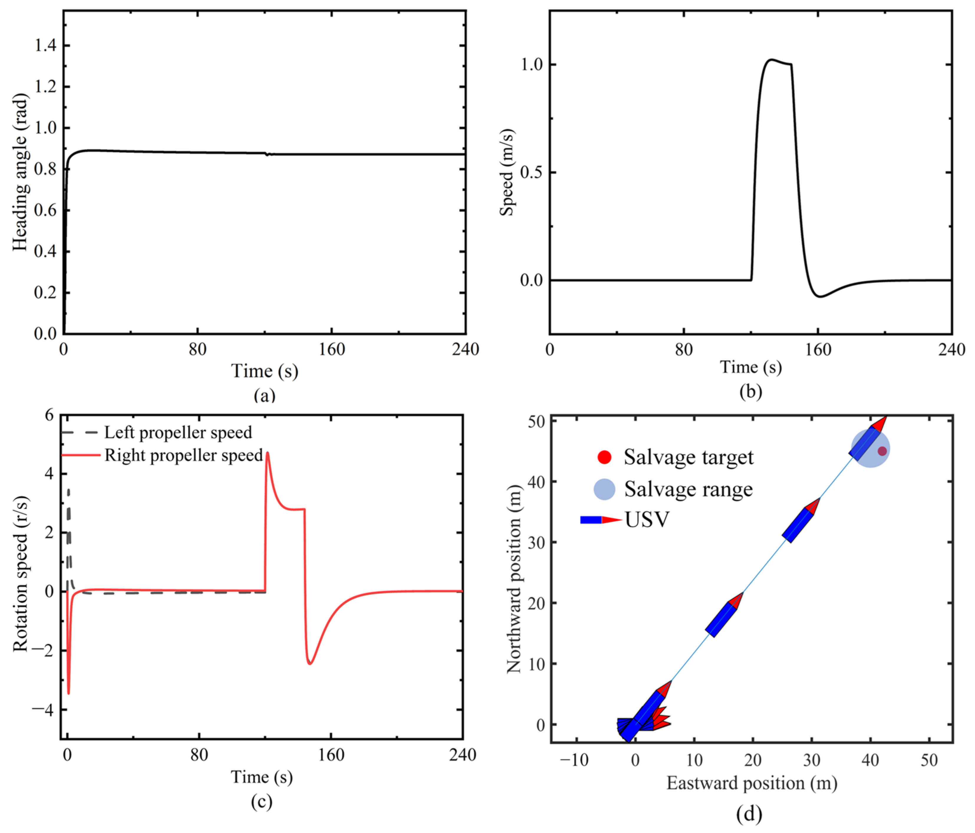
4.2.1. Heading and Speed Controller

Figure 12a shows the actual heading of the USV controlled by the heading and speed controller when the desired speed is 1 m/s. The actual heading of the USV follows a sine curve. The error between the actual heading and the desired heading fluctuates around 0 rad, and it is bounded. Figure 12b shows the rotational speeds of the left and right propellers. At the beginning of the simulation, the rotational speeds of the left and right propellers increase simultaneously; at this moment, the USV is in a state of linear acceleration. Subsequently, the rotational speeds of the left and right propellers fluctuate sinusoidally around 5 r/s, but the sum of the rotational speeds remains constant. Figure 12c shows the actual speed of the USV. The speed of the USV accelerates from 0 to 1 m/s. It can be seen from Figure 10 that the error between the actual heading and the desired heading of the USV is bounded, which proves that the proposed heading and speed controller can control the USV to track the desired heading.

Figure 13a shows the actual heading of the USV controlled by the heading and speed controller when the desired speed is 0 m/s. The actual heading of the USV follows a sine curve. The error between the actual heading and the desired heading fluctuates around 0 rad, and the amplitude of the fluctuation is greater than that of the simulation with a desired speed of 1 m/s. Figure 13b shows the rotational speeds of the left and right propellers. The left and right propellers start to rotate at the same speed, but in opposite directions, from the initial moment. Figure 13c shows the actual speed of the USV. The speed of the USV remains at zero all the time. As shown in Figure 11, the error between the actual heading and the desired heading of the USV is bounded, and the speed of the USV is zero. This indicates that the proposed heading and speed controller can control the USV to track the desired course when the speed of the USV is zero.

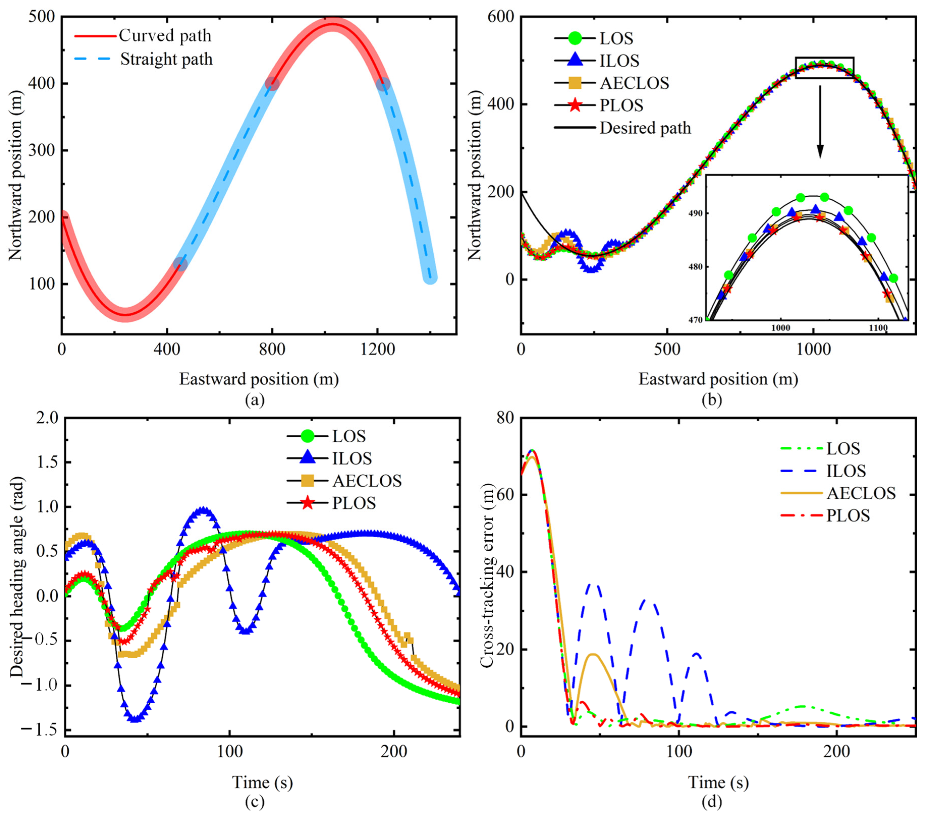
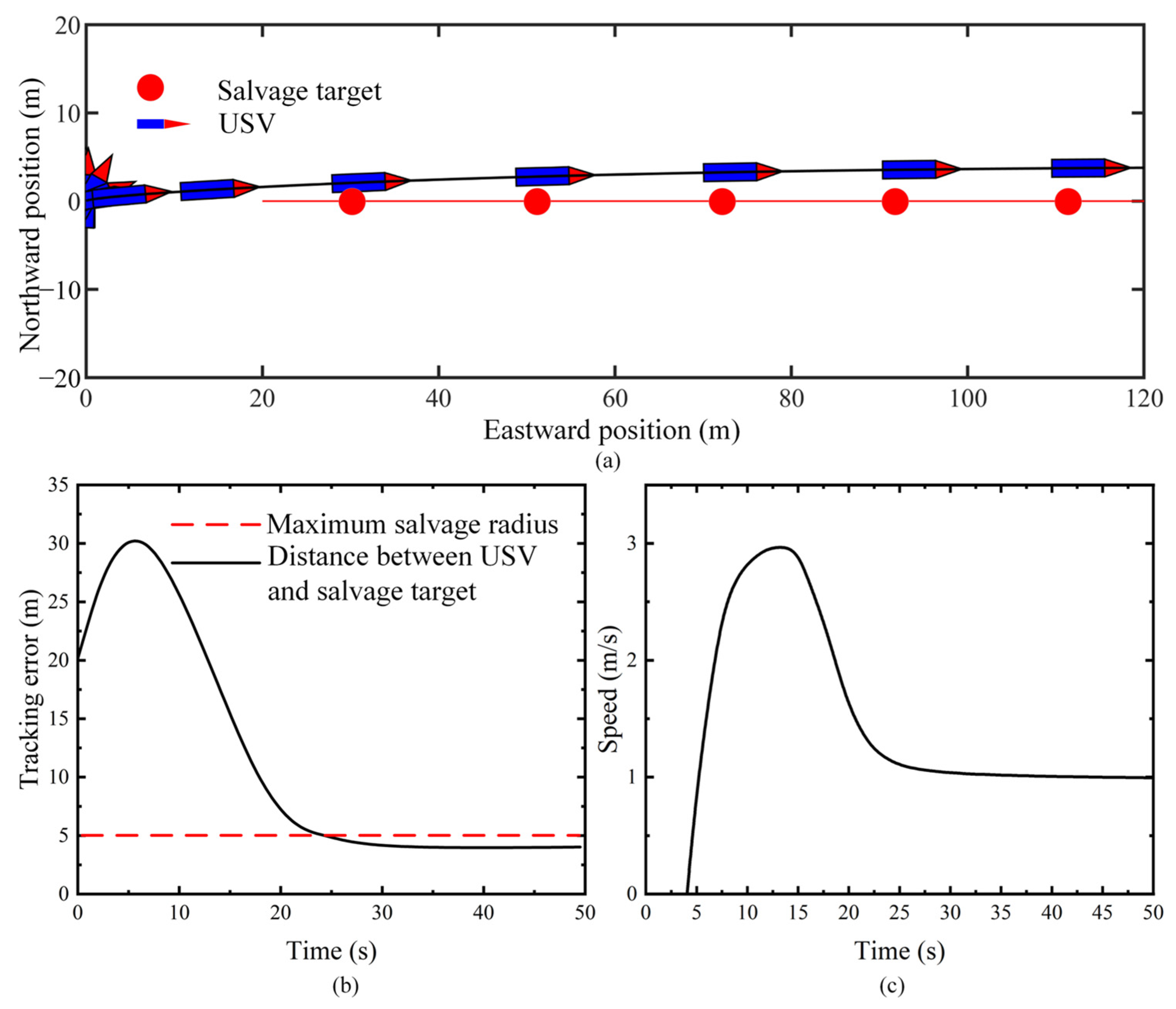
4.2.2. Rapid Approach Phase

Figure 14 shows the results for the USV following the interpolated curved path when guided by the LOS guidance algorithm, ILOS guidance algorithm, AECLOS guidance algorithm, and PLOS guidance algorithm. Figure 14a shows the segmentation of the path. Figure 14b shows the position of the USV during the path following. At the beginning of the path following, the USV when guided by the ILOS guidance algorithm and the AECLOS guidance algorithm exhibits overshoot. In contrast, the USV when guided by the LOS guidance algorithm and the PLOS guidance algorithm has a smooth trajectory. In the second segment of the curve path, the USV when guided by all four guidance algorithms exhibits cross-tracking error. When guided by the LOS guidance algorithm, the USV demonstrates the largest cross-tracking error. The cross-tracking error is the smallest when the USV is guided by the PLOS guidance algorithm.

Figure 14c shows the desired heading calculated by the four guidance algorithms. The desired heading calculated by the ILOS guidance algorithm has oscillations. The desired heading calculated by the LOS guidance algorithm is the smoothest. The desired heading calculated by the AECLOS and PLOS guidance algorithms has sudden changes. Figure 14d shows the cross-tracking error of the four guidance algorithms. Within 30 s, the cross-tracking error trends of the USV when guided by the four guidance algorithms are consistent. After 30 s, the cross-tracking error of the USV when guided by the ILOS guidance algorithm and the AECLOS guidance algorithm shows oscillation. The cross-tracking error of the USV when guided by the LOS guidance algorithm reaches a peak at 180 s.

Figure 15 shows the results for the USV following the Dubins path when guided by the LOS guidance algorithm, ILOS guidance algorithm, AECLOS guidance algorithm, and PLOS guidance algorithm. Figure 15a shows the segmentation of the path. Figure 15b shows the position of the USV during the path following under the guidance of four guidance algorithms. When transforming from the straight-line path segment to the curved path segment, the USV when guided by the LOS guidance algorithm, ILOS guidance algorithm, and AECLOS guidance algorithm moves along the original straight-line direction before it begins to converge toward the curve. The actual path of the USV under the guidance of the PLOS guidance algorithm fits the curve. Figure 15c shows the desired heading calculated by the four guidance algorithms. As shown in Figure 15c, the USV when guided by PLOS guidance algorithm changes course earlier than the other three algorithms. It shows that the USV is guided by the PLOS guidance algorithm in advance through the drift angle calculated by the model prediction. When the USV’s path transforms from the straight-line path to the curved path, when the drift angle is created by the PLOS guidance algorithm, the USV does not sail far out of the path. Figure 15d shows the cross-tracking error of the four guidance algorithms. It can be seen that when following the curved path segment, the USV guided by the LOS guidance algorithm has a steady-state cross-tracking error. The cross-tracking error of the USV when guided by the ILOS guidance algorithm and AECLOS guidance algorithm is gradually reduced.

The average cross-tracking error, the standard deviation of the cross-tracking error, and root mean square error of the cross-tracking error when the USV follows the interpolated curved path are given in

Table 3. Statistical results of cross-tracking error for USV following interpolated path.

Algorithm	Average (m)	Standard Deviation (m)	Root Mean Square Error (m)
LOS	8.144	21.844	22.114
ILOS	10.858	18.462	18.747
AECLOS	8.012	16.705	16.094
PLOS	6.602	17.703	13.212

. When following the interpolated curved path, the average cross-tracking error when using the PLOS guidance algorithm is reduced by 18.9%, 39.2%, and 17.6% compared with that obtained when using the LOS guidance algorithm, ILOS guidance algorithm, and AECLOS guidance algorithm, respectively. The standard deviation of the cross-tracking error when using the PLOS guidance algorithm is reduced by 19.0% and 4.1% compared with that obtained when using the LOS guidance algorithm and ILOS guidance algorithm, and 6.0% higher than that obtained when using the AECLOS guidance algorithm. The root mean square error when using the PLOS guidance algorithm is reduced by 40.3%, 29.5%, and 17.9% compared with that obtained when using the LOS guidance algorithm, ILOS guidance algorithm, and AECLOS guidance algorithm, respectively.

The average cross-tracking error, the standard deviation of the cross-tracking error, and root mean square error of the cross-tracking error when the USV follows the Dubins path are given in

Table 4. Statistical results of cross-tracking error for USV following Dubins path.

Algorithm	Average (m)	Standard Deviation (m)	Root Mean Square Error (m)
LOS	1.837	1.701	3.092
ILOS	0.972	1.020	2.154
AECLOS	0.519	0.730	1.782
PLOS	0.218	0.190	1.504

. When following the Dubins curved path, the average cross-tracking error when using the PLOS guidance algorithm is reduced by 88.1%, 77.6%, and 58% compared with that obtained when using the LOS guidance algorithm, ILOS guidance algorithm, and AECLOS guidance algorithm, respectively. The standard deviation of the cross-tracking error when using the PLOS guidance algorithm is reduced by 88.8%, 81.4%, and 74.0% compared with that obtained when using the LOS guidance algorithm, ILOS guidance algorithm, and AECLOS guidance algorithm. The root mean square error when using the PLOS guidance algorithm is reduced by 51.4%, 30.2%, and 15.6% compared with that obtained when using the LOS guidance algorithm, ILOS guidance algorithm, and AECLOS guidance algorithm, respectively. It can be concluded that the PLOS guidance algorithm has the smallest path cross-tracking error. This indicates that the tracking accuracy of the USV is improved when controlled by the PLOS guidance algorithm.

4.2.3. Terminal Tracking Phase

Figure 16 shows the results for the USV tracking a stationary salvage target. Figure 16a shows the actual heading of the USV. The results show that the actual heading of the USV converges at 0.87 rad. Figure 16b shows the actual speed of the USV. The USV has a speed of zero from 0 to 90 s. From 90 s to 160 s, the USV rapidly accelerates to a speed of 1 m/s, and then decelerates to zero. During 0–120 s, the USV adjusts its heading in place. After the system detects that the heading is stable, it starts to travel towards the key point at a speed of 1 m/s. When $\left|l_t-R_s\right|$ is less than 0.15 m, the USV brakes. Figure 16c shows the rotational speeds of the left and right propellers. Before 90 s, the left and right propellers rotate in opposite directions. After 90 s, the left and right propellers rotate at the same speed and in the same direction to generate propulsion. As shown in Figure 16d, the salvage target is on the starboard side of the USV, where the salvage actuator is installed. The distance between the USV and the target is 3.20 m, which is within the radius of the working space of the salvage actuator. This demonstrates that the key point guidance algorithm is capable of maintaining the stationary salvage target within the operational workspace of the salvage actuator.

Figure 17 shows the results for the USV tracking a moving salvage target. Figure 17a shows the position of the USV and the position of the salvage target. At the initial stage of the simulation, the USV adjusts its heading. Then it begins to move towards the salvage target, and finally it moves parallel to the salvage target. Figure 17b shows the tracking error of the USV. At the initial stage of the simulation, the distance between the USV and the salvage target keeps increasing. After 5.5 s, the distance between the USV and the salvage target reaches its maximum, and then gradually decreases. It finally converges around 3.9 m, which is within the salvage radius and meets the task requirements. Figure 17c shows the speed of the USV. The speed-limiting factor restricts the turning radius of the USV. At the initial stage of tracking, the speed of the USV is 0 m/s, and the distance between the salvage target and the USV gradually increases. When the heading converges, the USV starts to accelerate to track the salvage target. Finally, the speed of the USV is the same as that of the salvage target; the USV is moving in parallel with the salvage target.

The simulation results show that the proposed salvage target tracking algorithm can effectively track the salvage target and maintain the corresponding distance.

5. Experimental Verification

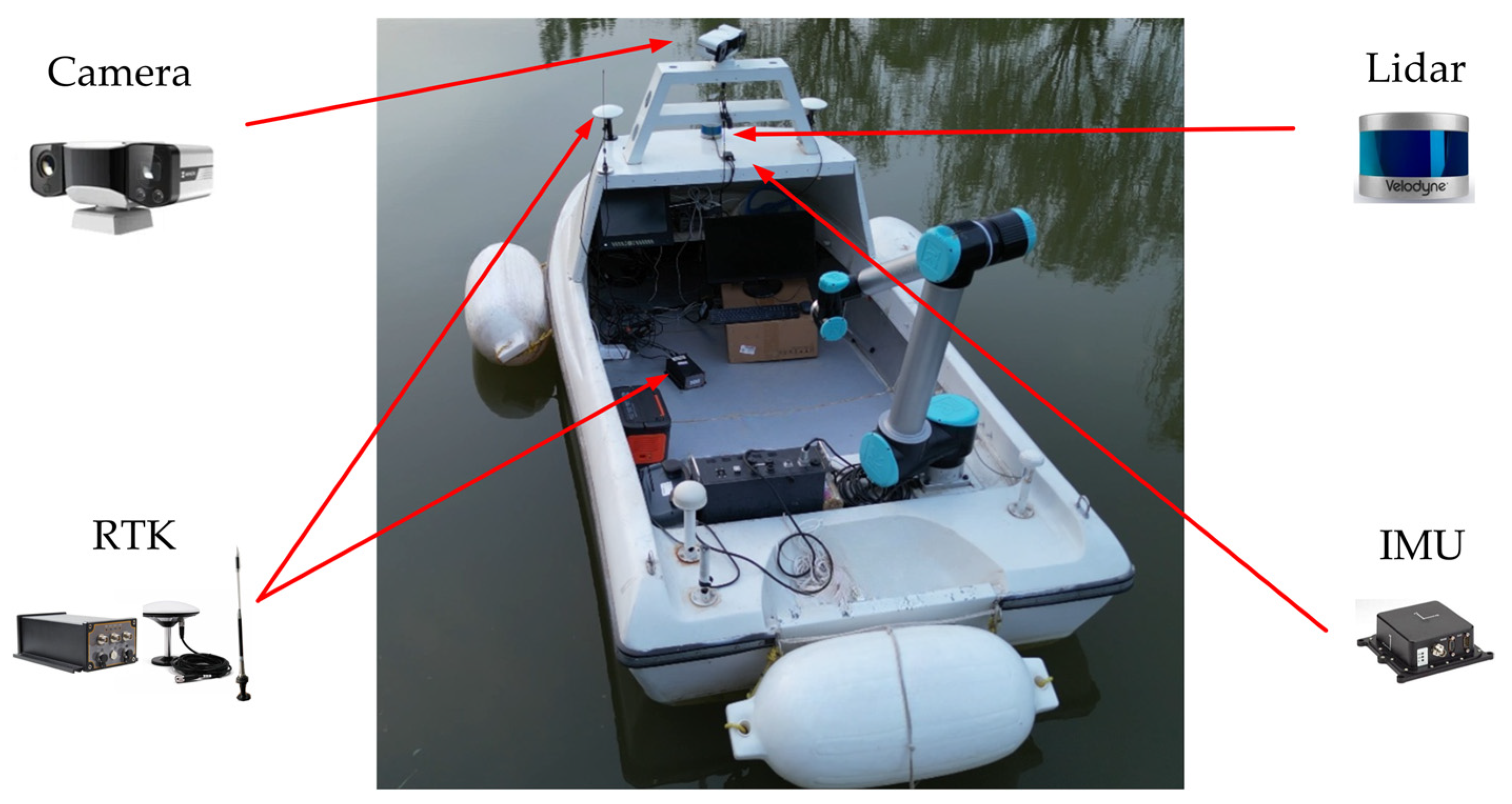
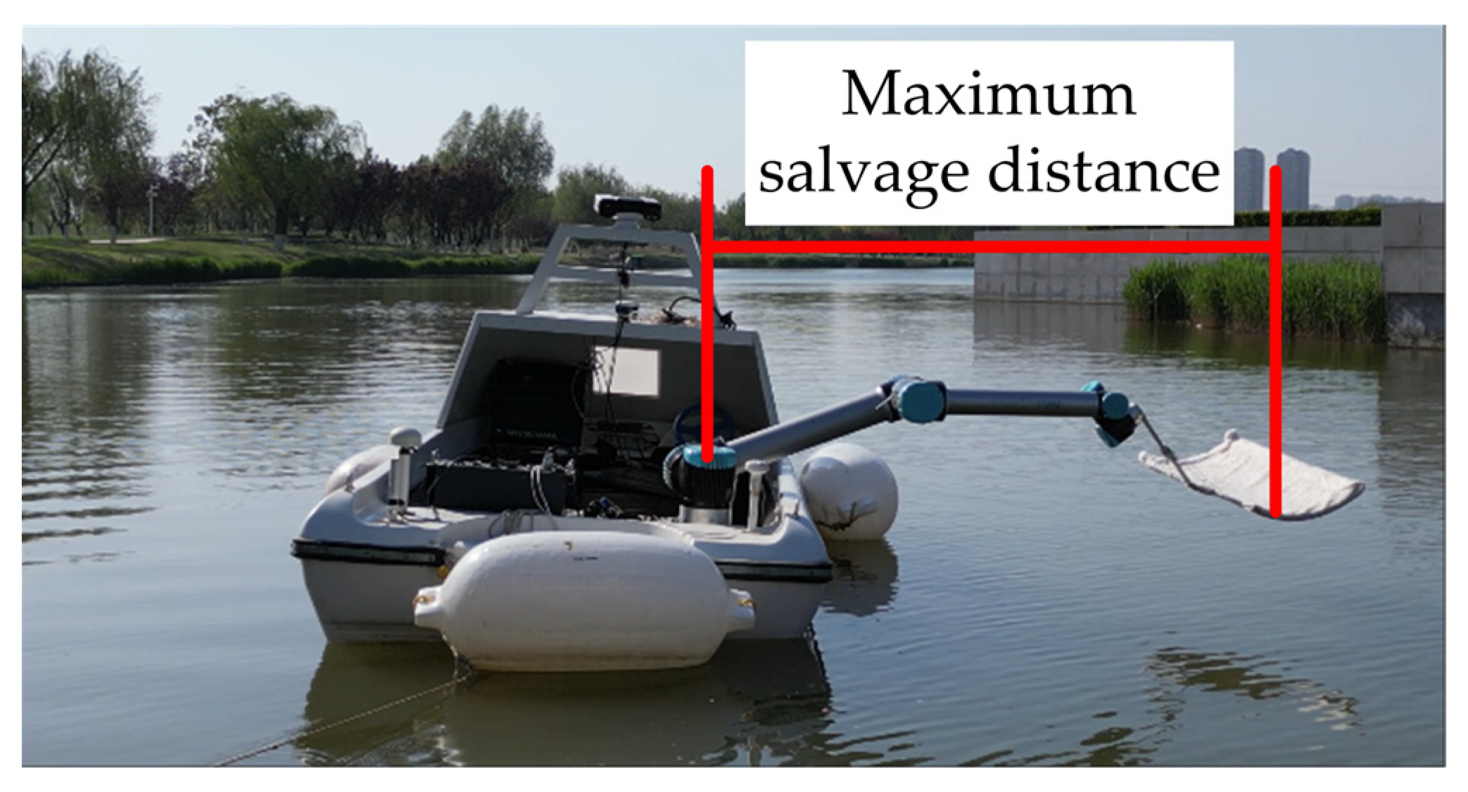
5.1. Experimental Platform

To validate the effectiveness of the proposed STT algorithm, an experimental platform was constructed based on a surface rescue USV, which is driven by dual propellers. As shown in Figure 18, the platform was equipped with a lidar, a visual camera, an inertial measurement unit (IMU), and an RTK positioning system. Specifically, the model of the lidar was VLP-16, and the model of the camera was HM-SF7353-W. The lidar and visual camera were employed to sample both the azimuth and the relative distance from the USV to the salvage target. The model of the IMU, which provided the heading and speed information of the USV, was SC-INS-200S, while the model of the RTK, which was employed to obtain the global position of the USV, was MC300. The main parameters of the USV are listed in

Table 5. Main parameters of experimental platform.

Parameter	Value
Length × width × height	4.80 m × 1.60 m × 0.90 m
Weight	550.00 kg
Load	500.00 kg
Draft depth	0.22 m
Distance between left and right propellers	1.30 m
Diameter of propellers	0.15 m
Advance coefficient of propellers	0.13
Maximum rotational speed of propellers under no-load condition	13.33 r/s
Coefficient of propellers influencing on turning moment	0.29

. A serial six-degree-of-freedom robotic arm was employed as the salvage actuator, which was mounted on the rear-right side of the USV. A schematic of the maximum working radius is shown in Figure 19, and measurements indicate that the maximum salvage distance was 2.13 m.

The experiment was conducted in an annular water system characterized by a stable water current. A rescue training dummy was used as the salvage target. The dummy was released into the center of the lake, allowing it to drift with the current. Subsequently, the autonomous control program of the USV was activated, in which the STT algorithm was implemented to guide the USV in tracking the drifting dummy.

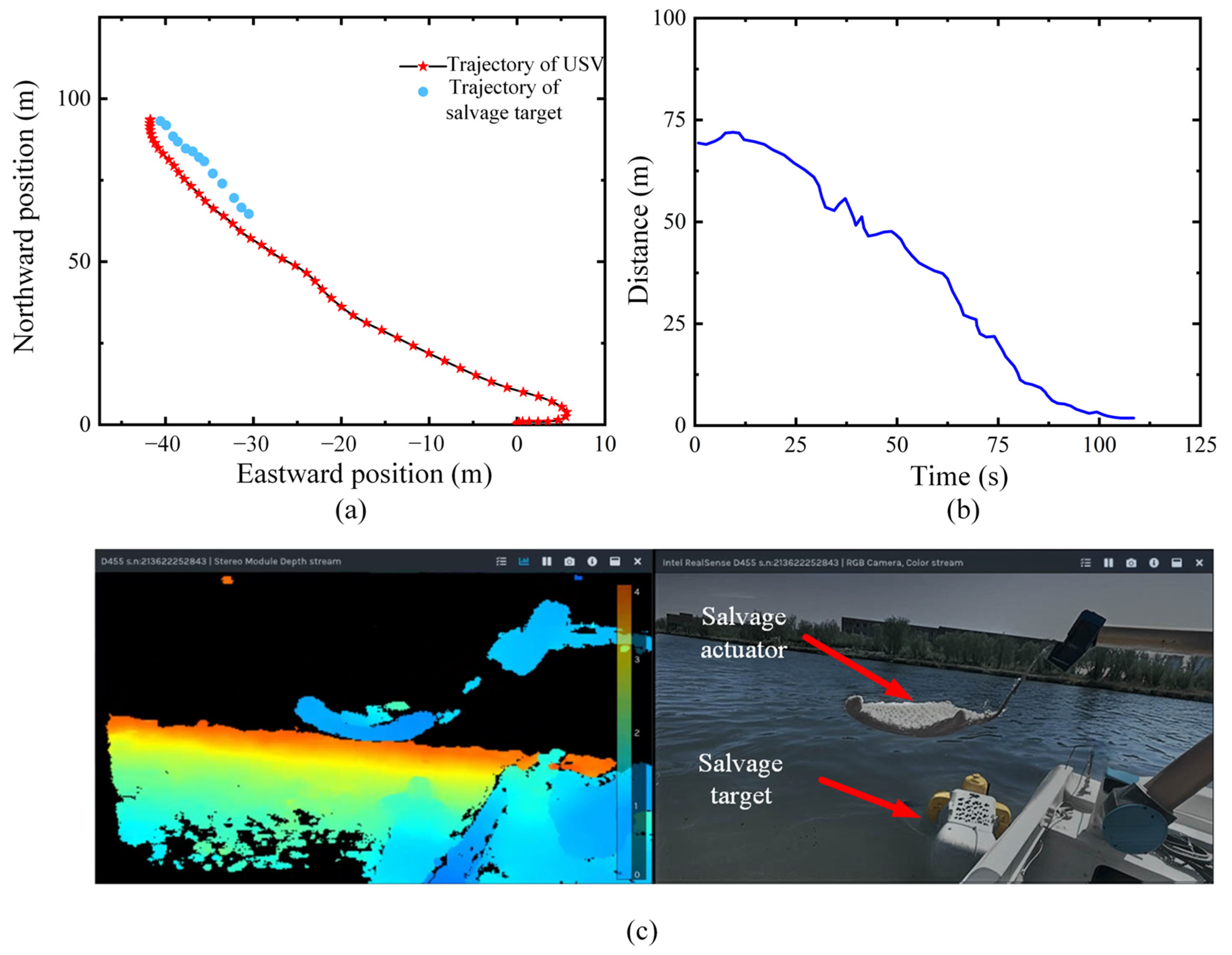
5.2. Experimental Results

Figure 20a shows the trajectories of the USV and the salvage target during the tracking process. Figure 20b shows the distance between the USV and the salvage target during the tracking process. The final distance stabilizes within 1.13 m, which is less than the maximum salvage range, thereby meeting the operational requirements for salvage operation. Figure 20c presents the relative positional relationship between the USV and the salvage target, as captured by the depth camera. From the depth image, it can be observed that the distance between the target and the camera is equal to the distance between the end-effector of the robotic arm and the camera. From the visual image, it can be observed that the target is located within the working space of the salvage actuator.

6. Conclusions

This paper proposes the salvage target tracking (STT) algorithm for tracking salvage targets, which is used to provide necessary support for the surface rescue tasks performed by twin-propeller and non-rudder unmanned surface vehicles. The algorithm consists of a rapid approach phase and a terminal tracking phase, according to the distance between the USV and the salvage target. When the distance between the USV and the salvage target is greater than 10 times the length of the USV, the salvage target tracking algorithm operates in the rapid approach phase. The PLOS guidance algorithm is applied in the rapid approach phase. When the distance between the USV and the salvage target is less than 10 times the length of the USV, it enters the terminal tracking phase. The key point guidance algorithm is proposed to track the salvage target. Moreover, a heading and speed controller with rotational speed as the input is designed, and all the control objectives of the salvage tracking algorithm are achieved by adjusting the rotational speeds of the left and right propellers.

Simulation experiments were conducted to verify the effectiveness of the STT algorithm. The effectiveness of the proposed heading and speed controller was verified. The results show that the heading and speed controller can track the time-varying heading while maintaining the cruising speed. The effect of the proposed PLOS guidance algorithm was verified by comparing it with three algorithms: the LOS guidance algorithm, the ILOS guidance algorithm, and the AECLOS guidance algorithm. The results show that the PLOS guidance algorithm proposed in this paper has the highest accuracy in path following. The key point guidance algorithm was verified. The results show that the USV can track the salvage target and maintain the corresponding distance. In general, the proposed salvage target tracking algorithm can achieve effective tracking of salvage targets, which will provide support for salvage tasks performed by USVs. Near-shore experiments were conducted to validate the effectiveness of the STT algorithm. The experimental results demonstrate that the USV successfully tracked the salvage target while maintaining a relative position that met the spatial constraints required for successful salvage operations under the guidance of the STT algorithm.

The salvage target tracking algorithm proposed in this paper only considers a single-target scenario. In the future, the use of the salvage target tracking algorithm for a multi-target scenario will be considered, and it is necessary to avoid obstacles during the tracking process. In addition, the STT algorithm does not sufficiently account for resistance to external environmental disturbances. Future work will focus on the design of adaptive control algorithms that take environmental disturbances into account, in order to enhance the robustness of the system.

References

1. Kim, J. Target following and close monitoring using an unmanned surface vehicle. IEEE Trans. Syst. Man Cybern. Syst. 2020, 50, 4233–4242. [Google Scholar] [CrossRef]
2. Maternová, A.; Materna, M.; Dávid, A.; Török, A.; Švábová, L. Human error analysis and fatality prediction in maritime accidents. J. Mar. Sci. Eng. 2023, 11, 2287. [Google Scholar] [CrossRef]
3. Xue, J.; Papadimitriou, E.; Reniers, G.; Wu, C.; Jiang, D.; van Gelder, P.H.A.J.M. A comprehensive statistical investigation framework for characteristics and causes analysis of ship accidents: A case study in the fluctuating backwater area of Three Gorges Reservoir region. Ocean Eng. 2021, 229, 108981. [Google Scholar] [CrossRef]
4. Breivik, M.; Hovstein, V.E.; Fossen, T.I. Straight-line target tracking for unmanned surface vehicles. Model. Identif. Control A Nor. Res. Bull. 2008, 29, 131–149. [Google Scholar] [CrossRef]
5. Liu, Z.; Wang, Y.; Han, Q. Adaptive fault-tolerant trajectory tracking control of twin-propeller non-rudder unmanned surface vehicles. Ocean Eng. 2023, 285, 115294. [Google Scholar] [CrossRef]
6. Fossen, T.I. Handbook of Marine Craft Hydrodynamics and Motion Control; John Wiley & Sons, Ltd.: Chichester, UK, 2011. [Google Scholar] [CrossRef]
7. Do, K.D.; Jiang, Z.P.; Pan, J. Robust adaptive path following of underactuated ships. Automatica 2004, 40, 929–944. [Google Scholar] [CrossRef]
8. Zhang, G.; Zhang, X. A novel DVS guidance principle and robust adaptive path-following control for underactuated ships using low frequency gain-learning. ISA Trans. 2015, 56, 75–85. [Google Scholar] [CrossRef]
9. Samson, C. Control of chained systems application to path following and time-varying point-stabilization of mobile robots. IEEE Trans. Autom. Control 1995, 40, 64–77. [Google Scholar] [CrossRef]
10. Skjetne, R.; Fossen, T.I. Nonlinear maneuvering and control of ships. In Proceedings of the MTS/IEEE Oceans 2001, Honolulu, HI, USA, 5–8 November 2001; pp. 1808–1815. [Google Scholar] [CrossRef]
11. Wan, L.; Su, Y.; Zhang, H.; Shi, B.; AbouOmar, M.S. An improved integral light-of-sight guidance algorithm for path following of unmanned surface vehicles. Ocean Eng. 2020, 205, 107302. [Google Scholar] [CrossRef]
12. Fossen, T.I.; Pettersen, K.Y.; Galeazzi, R. Line-of-sight path following for dubins paths with adaptive sideslip compensation of drift forces. IEEE Trans. Control Syst. Technol. 2015, 23, 820–827. [Google Scholar] [CrossRef]
13. Pettersen, K.Y.; Lefeber, E. Way point tracking control of ships. In Proceedings of the 40th IEEE Conference on Decision and Control, Orlando, FL, USA, 4–7 December 2001; pp. 940–945. [Google Scholar] [CrossRef]
14. Liu, C.; Negenborn, R.R.; Chu, X.; Zheng, H. Predictive path following based on adaptive line-of-sight for underactuated autonomous surface vessels. J. Mar. Sci. Technol. 2017, 23, 483–494. [Google Scholar] [CrossRef]
15. Khaled, N.; Chalhoub, N.G. A self-tuning guidance and control system for marine surface vessels. Nonlinear Dyn. 2013, 73, 897–906. [Google Scholar] [CrossRef]
16. Mu, D.; Wang, G.; Fan, Y.; Bai, Y.; Zhao, Y. Fuzzy-based optimal adaptive line-of-sight path following for underactuated unmanned surface vehicle with uncertainties and time-varying disturbances. Math. Probl. Eng. 2018, 2018, 7512606. [Google Scholar] [CrossRef]
17. Liu, C.; Chen, C.L.P.; Zou, Z.; Li, T. Adaptive NN-DSC control design for path following of underactuated surface vessels with input saturation. Neurocomputing 2017, 267, 466–474. [Google Scholar] [CrossRef]
18. Liu, L.; Wang, D.; Peng, Z. ESO-based line-of-sight guidance algorithm for path following of underactuated marine surface vehicles with exact sideslip compensation. IEEE J. Ocean. Eng. 2017, 42, 477–487. [Google Scholar] [CrossRef]
19. Qi, J.; Wang, B.; Fei, Q. Curve path following based on improved line-of-sight algorithm for USV. In Proceedings of the 2022 China Automation Congress, Xiamen, China, 25–27 November 2022; pp. 3801–3806. [Google Scholar] [CrossRef]
20. Maki, T.; Mizushima, H.; Kondo, H.; Ura, T.; Sakamaki, T.; Yanggisawa, M.; Yanagisawa, M. Real time path-planning of an AUV based on characteristics of passive acoustic landmarks for visual mapping of shallow vent fields. In Proceedings of the OCEANS 2007, Vancouver, BC, Canada, 29 September 2007–4 October 2007. [Google Scholar] [CrossRef]
21. Hernández, J.D.; Moll, M.; Vidal, E.; Carreras, M.; Kavraki, L. Planning feasible and safe paths online for autonomous underwater vehicles in unknown environments. In Proceedings of the 2016 IEEE/RSJ International Conference on Intelligent Robots and Systems, Daejeon, Republic of Korea, 9–14 October 2016. [Google Scholar] [CrossRef]
22. Svec, P.; Shah, B.C.; Bertaska, I.R.; Alvarez, J.; Sinisterra, A.J.; Ellenrieder, K.V. Dynamics-aware target following for an autonomous surface vehicle operating under COLREGs in civilian traffic. In Proceedings of the 2013 IEEE/RSJ International Conference on Intelligent Robots and Systems, Tokyo, Japan, 3–7 November 2013; pp. 3871–3878. [Google Scholar] [CrossRef]
23. Chen, Z.; Zhang, Y.; Zhang, Y.; Nie, Y.; Tang, J.; Zhu, S. A hybrid path planning algorithm for unmanned surface vehicles in complex environment with dynamic obstacles. IEEE Access 2019, 7, 126439–126449. [Google Scholar] [CrossRef]
24. Singh, Y.; Sharma, S.; Sutton, R.; Hatton, D.; Khan, A. Feasibility study of a constrained Dijkstra approach for optimal path planning of an unmanned surface vehicle in a dynamic maritime environment. In Proceedings of the 2018 IEEE International Conference on Autonomous Robot Systems and Competitions, Torres Vedras, Portugal, 25–27 April 2018; pp. 117–122. [Google Scholar] [CrossRef]
25. Wang, D.; Wang, P.; Zhang, X.; Guo, X.; Shu, Y.; Tian, X. An obstacle avoidance strategy for the wave glider based on the improved artificial potential field and collision prediction model. Ocean Eng. 2020, 206, 107356. [Google Scholar] [CrossRef]
26. Du, B.; Xie, W.; Zhang, W.; Chen, H. A target tracking guidance for unmanned surface vehicles in the presence of obstacles. IEEE Trans. Intell. Transp. Syst. 2024, 25, 4102–4115. [Google Scholar] [CrossRef]
27. Zhang, M.; Zheng, X.; Wang, J.; Pan, Z.; Che, W.; Wang, H. Trajectory planning for cooperative double unmanned surface vehicles connected with a floating rope for floating garbage cleaning. J. Mar. Sci. Eng. 2024, 12, 739. [Google Scholar] [CrossRef]
28. Sun, P.; Zhu, B.; Zuo, Z.; Basin, M.V. Vision-based finite-time uncooperative target tracking for UAV subject to actuator saturation. Automatica 2021, 130, 109708. [Google Scholar] [CrossRef]
29. Aumtab, C.; Wanichanon, T. Stability and tracking control of nonlinear rigid-body ship motions. J. Mar. Sci. Eng. 2022, 10, 153. [Google Scholar] [CrossRef]
30. Liu, H.; Lin, J.; Yu, G.; Yuan, J.; Precup, R.E. Robust adaptive self-structuring neural network bounded target tracking control of underactuated surface vessels. Comput. Intell. Neurosci. 2021, 2021, 2010493. [Google Scholar] [CrossRef] [PubMed]
31. Shojaei, K. Three-dimensional neural network tracking control of a moving target by underactuated autonomous underwater vehicles. Neural Comput. Appl. 2017, 31, 509–521. [Google Scholar] [CrossRef]
32. Kim, J. Optimal motion controllers for an unmanned surface vehicle to track a maneuvering underwater target based on coarse range-bearing measurements. Ocean Eng. 2020, 216, 107973. [Google Scholar] [CrossRef]
33. ISO 11592-1:2016; Small Craft—Determination of Maximum Propulsion Power Rating Using Planing Test Method—Part 1: Craft Designed for A Maximum Engine Power Level of 110 kW and Above. British Standards Institution. International Organization for Standardization: Geneva, Switzerland, 2016.
Figure 1. Schematic diagram of USV and salvage actuator. (a) Body-fixed coordinate system and global coordinate system; (b) workspace of salvage actuator; (c) position of left and right propellers.
Jmse 13 01158 g001
Figure 2. Dynamic model of twin-propeller and non-rudder USV.
Jmse 13 01158 g002
Figure 3. Schematic diagram of salvage target tracking algorithm.
Jmse 13 01158 g003
Figure 4. Diagram of path-following system based on line-of-sight guidance.
Jmse 13 01158 g004
Figure 5. Comparison of line of sight obtained with improved line-of-sight guidance algorithm based on model prediction (a) without drift angle compensation, and (b) with drift angle compensation.
Jmse 13 01158 g005
Figure 6. Schematic diagram of key point guidance algorithm. (a) Key point guidance algorithm for stationary salvage target; (b) key point guidance algorithm for moving salvage target.
Jmse 13 01158 g006
Figure 7. Flowchart of key point guidance algorithm for stationary salvage target.
Jmse 13 01158 g007
Figure 8. Schematic diagram of moving-target tracking with and without speed-limiting factor. (a) Moving-target tracking without speed-limiting factor. (b) Moving-target tracking with speed-limiting factor.
Jmse 13 01158 g008
Figure 9. Function graph of speed-limiting factor.
Jmse 13 01158 g009
Figure 10. Schematic diagram of heading and speed controller.
Jmse 13 01158 g010
Figure 11. Flowchart of salvage target tracking algorithm.
Jmse 13 01158 g011
Figure 12. Results of heading and speed controller at 1 m/s. (a) Actual heading and heading error of USV; (b) speed of left and right propellers; (c) speed of USV in surge direction.
Jmse 13 01158 g012
Figure 13. Results of heading and speed controller at 0 m/s. (a) Actual heading and heading error of USV; (b) speed of left and right propellers; (c) speed of USV in surge direction.
Jmse 13 01158 g013
Figure 14. Results diagram for USV following interpolated path guided by LOS guidance algorithm, ILOS guidance algorithm, AECLOS guidance algorithm, and PLOS guidance algorithm. (a) Path segmentation; (b) position; (c) desired heading; (d) cross-tracking error.
Jmse 13 01158 g014
Figure 15. Results diagram for USV following Dubins path when guided by LOS, ILOS, AECLOS, and PLOS guidance algorithms. (a) Path segmentation; (b) position; (c) desired heading; (d) cross-tracking error.
Jmse 13 01158 g015
Figure 16. Results of tracking stationary salvage target. (a) Heading of USV; (b) surge speed; (c) rotational speeds of left and right propellers; (d) position of USV and salvage target.
Jmse 13 01158 g016
Figure 17. Results for USV tracking moving salvage target. (a) Position of USV and salvage target; (b) distance between USV and salvage target; (c) surge speed of USV.
Jmse 13 01158 g017
Figure 18. Experimental platform for salvage.
Jmse 13 01158 g018
Figure 19. Schematic of maximum working radius.
Jmse 13 01158 g019
Figure 20. Results of salvage target tracking. (a) Trajectory of USV and salvage target; (b) distance between USV and salvage target; (c) relative positional relationship between USV and salvage target.
Jmse 13 01158 g020