Research on an Ice-Breaking Mechanism Using Subglacial Resonance

Abstract

The Arctic ice layer serves as an excellent cover for strategic nuclear submarine forces, but it also poses significant challenges when submarines surface. This paper proposes a method for breaking through the ice layer and surfacing in polar environments based on the principle of resonance. This method eliminates the need for direct contact between the submarine and the ice layer, solving the current issues with submarine ice-breaking methods that demand high strength from the submarine and pose risks to both the submarine and its crew. Through theoretical analysis, numerical simulation and experimental verification, the vibration characteristics and fracture mechanism of the ice layer under the action of excitation loads were studied. Experiments showed that when the excitation frequency matched the fundamental eigenfrequency Ω1 of the ice layer, obvious resonance occurred and cracks appeared in the ice layer. A dynamic model of the ice layer was established using Abaqus software, and modal extraction and stress analysis were carried out. The error between the Ω1 obtained by numerical simulation and the experimental results was only 0.53%, verifying the reliability of the model. After applying the excitation load with a frequency of Ω1, the stress in the ice layer gradually expanded to the strength limit of the ice, achieving an ice-breaking effect consistent with the experimental results. Experimental and simulation results showed that the use of Ω1 for resonance ice-breaking had the best effect. When the ice layer resonated, the stress increased first and then stabilized, and cracks occurred before the stress stabilized to achieve the ice-breaking effect.

1. Introduction

With the continuous development of polar marine areas and the expansion of polar trade routes by various countries, the potential for civil and military demands in the polar marine areas in the future is huge. Military powers will inevitably strengthen their military deployment in the polar regions. In particular, the thick ice layer in the polar region provides good concealment and survivability for underwater vehicles such as submarines. Future polar maritime operations will surely become a key direction for countries to focus on. The sound of polar sea ice melting and colliding can easily mask the noise generated by submarines, greatly increasing their concealment. However, in the ice-covered areas of the Arctic sea, submarines need to break through the ice to surface when performing tasks or encountering emergencies, which is a huge challenge to the safety of submarines. To improve the underwater combat performance of submarines in the polar region, it is essential to enhance their ice-breaking capabilities.

At present, the more mature ice-breaking methods include static loading ice-breaking and dynamic impact ice-breaking [1,2,3]. The former gradually discharges ballast water with compressed air, slowly increasing buoyancy and causing the ice layer to bend and break under continuous pressure. It is suitable for thicker ice layers and requires a slow and controllable ice-breaking process. The latter relies on the kinetic energy of the submarine’s hull to impact the ice layer during high-speed surfacing, depending on the high-strength steel reinforced conning tower and the forward structure of the hull. It is suitable for thinner ice layers or tactical scenarios requiring rapid breakthroughs. However, both methods mainly rely on the structural strength of the submarine itself and have relatively high cost efficiency. Therefore, it is necessary to propose a more efficient and safe ice-breaking method. Submarines and ice layers can be regarded as a vibration system, so resonance ice-breaking has gradually begun to be explored as an efficient ice-breaking technology.

Resonance ice-breaking was first observed as a phenomenon by Engelbrektson in 1983. Subsequently, Määttänen and other researchers [4] conducted in-depth analysis of the dynamic interaction between ice and structures, proposing the dynamic interaction mechanism between ice layers and structures during continuous crushing processes. Tsuchiya et al. [5] experimentally studied the interaction between ice and structures, providing experimental data for understanding the forces exerted by ice layers on structures. Based on this, Matlock et al. [6]. established an analytical model for the interaction between ice and structures, laying the foundation for subsequent theoretical research. Toyama et al. [7] experimentally studied the self-excited vibration of cylindrical structures under the action of ice layers and further analyzed the impact of this vibration on structures. Resonance ice-breaking was first applied to roads. Zhang and Wang [8] applied the resonance ice-breaking mechanism to the design of road deicing equipment. By adjusting the vibration frequency to match the natural frequency of the ice layer, efficient deicing was achieved. In the aerospace field, Kandagal and Venkatraman [9] used piezoelectric elements to study the resonance modes of cantilever plates in the low-frequency range and selected the mode with the maximum shear stress for excitation, achieving good deicing results. In addition, resonance ice-breaking has been applied in various scenarios, but the problems solved are mostly related to ice on structural surfaces [10,11,12]. In the polar context, Dai Huiling et al. [13] proposed a new type of polar ice-breaking method based on resonance theory and verified its feasibility and effectiveness through vibration characteristic analysis and numerical simulation. The research results show that by selecting appropriate vibration modes, excitation positions, and excitation amounts, efficient directional ice-breaking effects can be achieved. In addition, sea ice is regarded as a brittle material due to its material properties. However, there are relatively few studies on the constitutive model and damage model of ice. Therefore, when studying ice-breaking problems, relevant research on concrete, which is also a brittle material, can be referred to, such as the basic concepts of wave dispersion and dynamics in the classic non-local damage model, and the fracture analysis of concrete [14,15].

The above studies show that the application of resonance ice-breaking methods in roads, aviation, and ice is quite mature, but the methods are not suitable for the working conditions of breaking polar ice from underwater. Therefore, this paper applies the resonance ice-breaking method to large-scale planar ice-breaking under ice and conducts vibration characteristic analysis and numerical simulation of the ice-breaking process to explore the feasibility of resonance ice-breaking.

2. Basic Analysis of the Resonance Ice-Breaking Mechanism

When a submarine surfaces through ice, the sea ice can be regarded as an infinite plane. Due to the elastic effects of the structure and the ice layer, the excitation source and the ice layer constitute a vibration system. When the excitation source vibrates, energy is transmitted from the contact area to the entire ice layer. Most of the energy is stored as elastic strain energy, and the ice layer initially begins to vibrate slightly. As the duration of action increases, energy gradually accumulates and the amplitude of the entire ice layer gradually expands, eventually exceeding the elastic limit of the ice, resulting in fracture and completion of ice-breaking. The entire process is shown in Figure 1.

The ice layer in the polar environment is inhomogeneous, with different sizes and thicknesses. The elastic modulus and density of the ice layer in different areas are factors that need to be considered. This paper focuses on the ice-breaking mechanism under ice, so the ice layer has been simplified to a large plate single-degree-of-freedom system as shown in Figure 2. The ice layer is a two-dimensional plane supported arbitrarily on all four sides. For the actual underwater resonance excitation ice-breaking, the excitation point is relatively small compared to the entire ice layer. Therefore, to conduct basic research, the excitation has been set as a point acting on the center of the ice layer, with the force being F(t) [16].

The general equation of motion under the excitation of F(t) is [17,18]:

$$\begin{array}{l}D{\nabla }^{4}z+\rho h{\displaystyle \frac{{\partial }^{2}z}{\partial t^2}}+c{\displaystyle \frac{\partial z}{\partial t}}+kz=F(t)\\ D={\displaystyle \frac{E{h}^3}{12(1-{\mu }^2)}}\\ {\nabla }^4={\displaystyle \frac{{\partial }^4}{\partial x^2}}+{\displaystyle \frac{2{\partial }^4}{\partial x^2\partial y^2}}+{\displaystyle \frac{{\partial }^4}{\partial y^2}}\end{array}$$

(1)

In the equation, $D$, $E$, $\mu$, $\rho$, ${\nabla }^4$, $z$ represent the bending stiffness, elastic modulus, Poisson’s ratio, density, Laplacian operator, and displacement in the z-direction of the ice layer, respectively.

The solution for the natural frequency of the system is based on free vibration without considering damping, therefore, ($F(t)$ = 0) and ($c$) are generally neglected. Hence, the undamped motion differential equation for the ice layer performing free vibration on an elastic foundation is:

$$D{\nabla }^{4}z+\rho h{\displaystyle \frac{{\partial }^{2}z}{\partial t^2}}+kz=0$$

(2)

The strain energy generated by the bending of a rectangular thin plate is expressed as shown in Equation (3):

$$\begin{array}{l}{V}_p={\displaystyle \frac{1}{2}}D{\int }_0^a{\int }_0^b[{\left({\displaystyle \frac{{\partial }^{2}w(x,y,t)}{{\partial }^{2}x}}\right)}^2+{\left({\displaystyle \frac{{\partial }^{2}w(x,y,t)}{{\partial }^{2}y}}\right)}^2+\\ 2\mu \left({\displaystyle \frac{{\partial }^{2}w(x,y,t)}{{\partial }^{2}x}}\right)\left({\displaystyle \frac{{\partial }^{2}w(x,y,t)}{{\partial }^{2}y}}\right)+2(1-\mu ){\left({\displaystyle \frac{{\partial }^{2}w(x,y,t)}{\partial x\partial y}}\right)}^2]\mathrm{d}x\mathrm{d}y\end{array}$$

(3)

The elastic potential energy stored in the boundary springs of a rectangular thin plate is expressed as shown in Equation (4).

$$\begin{array}{c}{V}_s={\displaystyle \frac{1}{2}}{\int }_0^a{\left[k_{y0}w{(x,y,t)}^2+K_{y0}{\left({\displaystyle \frac{\partial w(x,y,t)}{\partial y}}\right)}^2\right]}_{y=0}\mathrm{d}x+\\ {\displaystyle \frac{1}{2}}{\int }_0^a{[k_{yb}w{(x,y,t)}^2+K_{yb}{({\displaystyle \frac{\partial w(x,y,t)}{\partial y}})}^2]}_{y=b}\mathrm{d}x+\\ {\displaystyle \frac{1}{2}}{\int }_0^b{[k_{x0}w{(x,y,t)}^2+K_{x0}{({\displaystyle \frac{\partial w(x,y,t)}{\partial x}})}^2]}_{x=0}\mathrm{d}y+\\ {\displaystyle \frac{1}{2}}{\int }_0^b{[k_{xa}w{(x,y,t)}^2+K_{xa}{({\displaystyle \frac{\partial w(x,y,t)}{\partial x}})}^2]}_{x=a}\mathrm{d}y\end{array}$$

(4)

The kinetic energy T of the rectangular thin plate system is expressed as:

$$T={\displaystyle \frac{1}{2}}\rho h{\int }_0^a{\int }_0^b({\begin{array}{c}\partial w(x,y,t)/\partial t)\end{array}}^2\mathrm{d}x\mathrm{d}y$$

(5)

The Lagrangian function for the rectangular thin plate is given by:

$$L=V_o+V_s-T$$

(6)

Finally, according to Hamilton’s principle, the matrix equation can be obtained as shown in Equation (7).

$$([K]-{\omega }_i^2[M])\{B\}=0$$

(7)

For the specific form of the matrix in the equation, refer to the summary by Lv et al. [19]. By solving Equation (7), the natural frequency and mode shape of the rectangular thin plate can be obtained. When the excitation frequency of the structure is close to the natural frequency of the ice [8], the amplitude of the vibration system’s response increases rapidly, which significantly increases the internal stress of the ice layer. When the stress exceeds the elastic limit of the ice layer, the ice layer will break.

3. Resonance Ice-Breaking Experiments and Numerical Simulations

The mechanical behavior of sea ice is very complex under the action of force. Accurately evaluating the force on the ice under resonance is of great significance for submarine missions. Considering economy and effectiveness, numerical simulation is an effective method for studying resonance ice-breaking and has been used to calculate the ice load under various ice conditions. Xue et al. [20]. studied the thickness and strength of ice in the Arctic shipping routes for a year, providing a basis for numerical simulation calculations. From a mechanical point of view, sea ice exhibits material properties similar to those of metals. However, the unique physical properties of sea ice distinguish it from ordinary metals. The grain size of ice is relatively large, making it difficult to homogenize at the microscopic structural level. Moreover, ice is prone to melting within the normal temperature range, which also increases the complexity of the mechanical behavior of sea ice.

3.1. Ice Layer Design, Finite Element Modeling, and Modal Numerical Analysis

Considering laboratory conditions such as the power of the exciter, low-temperature environment settings, and the size of the ice-making machine, the ice layer used in this study was designed to be 80 cm × 80 cm in size with a thickness of 1 cm. Based on the team’s previous research on ice-making methods, a saline solution with a mass fraction of 0.4% NaCl was selected to freeze and prepare the ice layer. Under this salinity, the expansion rate during freezing is relatively low, and the ice layer is less likely to develop numerous internal cracks due to freezing stress. During the ice layer preparation, the solution was slowly poured into an 80 cm × 80 cm mold. After degassing by standing still, the mold was placed into the ice-making machine and frozen at −10 °C for 24 h. At this point, the mechanical properties of the ice layer were not yet stable, but it was easy to demold. After demolding, the 1-cm-thick ice layer was placed back into the ice-making machine and frozen at −30 °C for another 3 days to stabilize its mechanical properties. The material parameters of the ice, which were determined by the team’s previous measurements under this preparation process and combined with existing literature for finite element simulation [21,22], are shown in

Table 1. Material Properties of the Ice Layer.

Density (kg/m3)	Elastic Modulus (GPa)	Poisson’s Ratio	Ultimate Strength (MPa)
816	10	0.33	1.8

.

In this study, the Abaqus 6.14 finite element simulation software was used for simulation research. Since finite element simulation has difficulty in effectively analyzing the mechanical behavior of an infinitely large and inhomogeneous ice layer numerically, the model was simplified to a two-dimensional large plane model, as shown in Figure 3. The ice layer plane was divided into three regions: Region I was set as the actual experimental support area, Region II was the mesh refinement area, and symmetrical boundaries were applied around the periphery.

The vibration modes of the ice layer plane were calculated and analyzed. Figure 4 shows the three basic mode shapes and natural frequencies of the ice layer plane. It can be seen from Figure 4 that at higher frequencies, the modal shape of the ice layer was more complex, and more energy was attenuated. For the entire vibration system, when the excitation position was at the peak or trough of the modal shape, it was easier to excite the corresponding mode, thereby more easily inducing resonance. Due to the limitations of the experimental equipment, it was only possible to output a sufficient excitation load at lower frequencies to achieve resonance of the ice layer. Therefore, in the subsequent experimental stage, only the vibration response analysis and resonance damage experiment for the 1st × 1st mode were conducted.

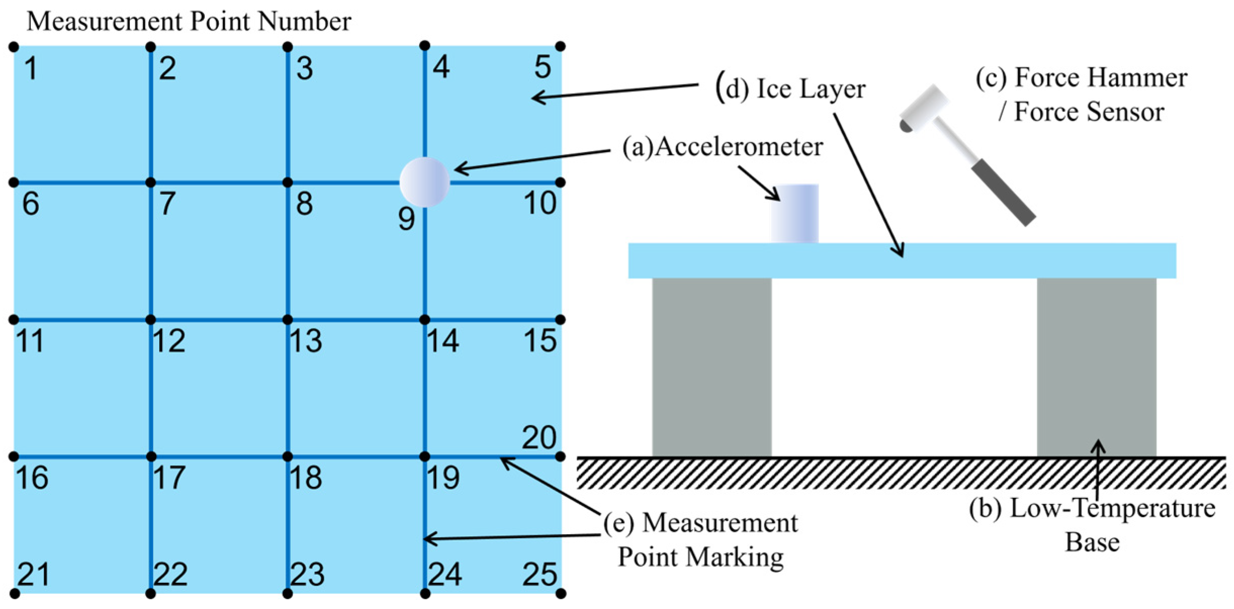
3.2. Natural Frequency Experiment of the Ice Layer

In order to study the vibration characteristics of the ice layer and determine the natural frequencies and corresponding modes of a specific ice layer, a natural frequency experiment was conducted on the specific ice layer using the impact method. The experimental setup is shown in Figure 5 and Figure 6. In the setup, (a) was the accelerometer, the base of which was frozen together with the ice layer and closely adhered to it through the freezing adhesion; (b) was the base that supported the ice layer plane. The base was hollow and contained ice that was frozen together with the ice layer. It was frozen simultaneously and at the same temperature as the ice layer, providing a low-temperature environment while supporting the ice layer; (c) was the force hammer, the head of which was connected to a force sensor for collecting force signals during the impact; (d) was the 80 cm × 80 cm ice layer, on which 25 measurement points in a 5 × 5 grid were marked by evenly drawing lines along two directions on the sides of the ice layer using pigment, as shown in (e).

Two hours before the experiment, the sensor base was placed into the ice-making machine to cool down and was frozen and bonded to the surface of the ice layer. Before the experiment began, the ice layer was taken out of the ice-making machine along with the sensor base and placed steadily on the low-temperature base. The accelerometer was then installed, and it was connected to the force hammer and the DHDAS dynamic signal acquisition and analysis system.

To ensure a tight bond between the accelerometer base and the ice layer, thereby ensuring the authenticity of the acceleration data, the position of the accelerometer base was not moved. The impact method experiment was conducted using a multi-point excitation and single-point response approach. The 25 measurement points were successively impacted, with three sets of highly coherent response data being stored for each point. After the testing was completed, the data were analyzed to obtain the modal shapes of the ice layer, as shown in Figure 7. These include the typical 1st × 1st modal shape shown in Figure 7a, with a natural frequency of 257.798 Hz for the ice layer in this mode; another typical 1st × 1st modal shape, shown in Figure 7b, with a natural frequency of 325.761 Hz for the ice layer in this mode; and the frequency response curve of the ice layer, shown in Figure 7c.

As shown in

Table 2. Comparison of experimental and simulation results.

1 cm Ice Layer Modal Analysis	Experimental Modal Frequency (Hz)	Simulated Modal Frequency (Hz)	Relative Error
1st × 1st	257.798	259.18 Hz	0.53%
1st × 2nd	325.761	383.20 Hz	14.937%

, the comparison between the numerical simulation results and the experimental results reveals that the relative error in the modal analysis was within 15%. Therefore, the numerical simulation method adopted in this paper is highly accurate and reliable. This method can be used to calculate the response and stress of the ice layer under excitation loads with a high degree of confidence. However, in subsequent studies, the size effect should be considered for the accuracy of numerical simulation [23].

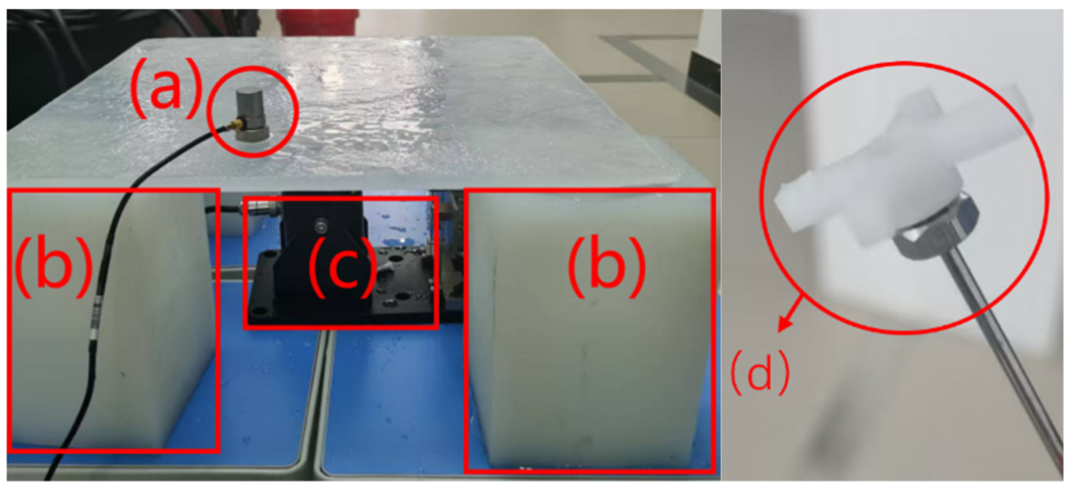
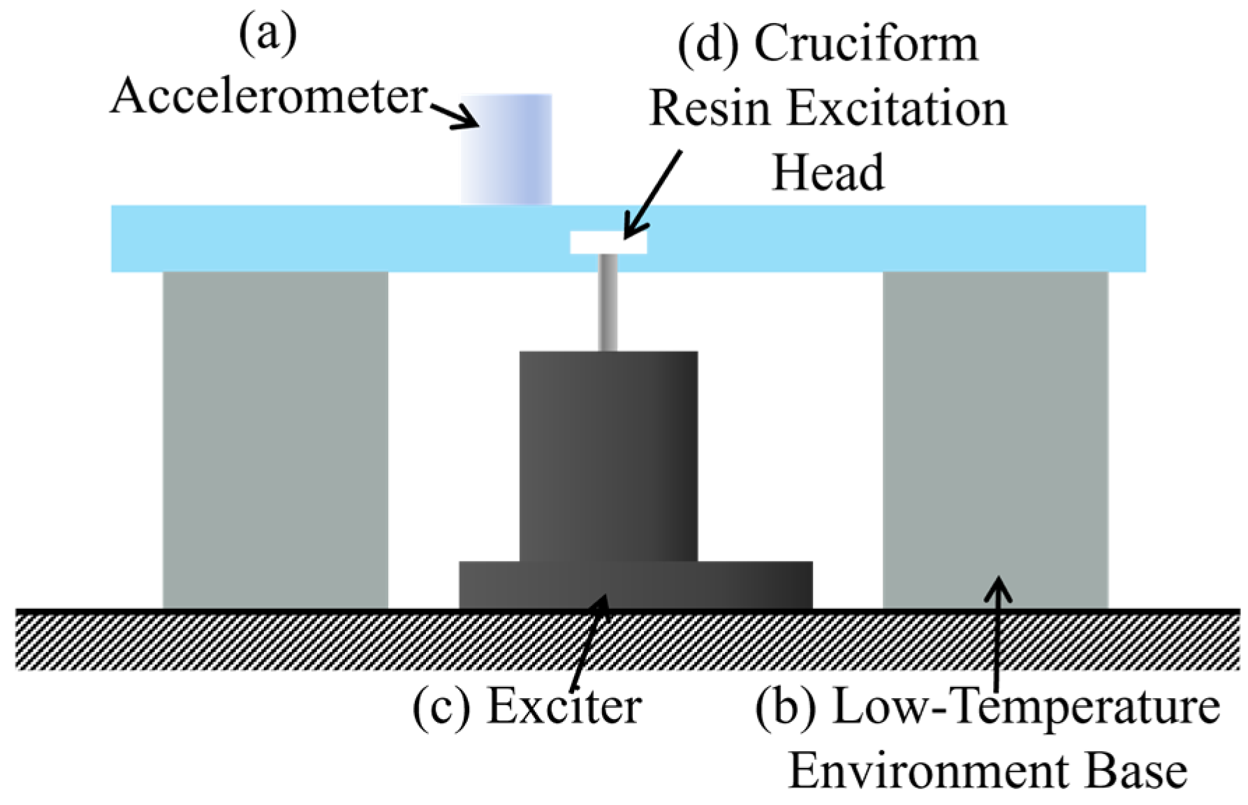
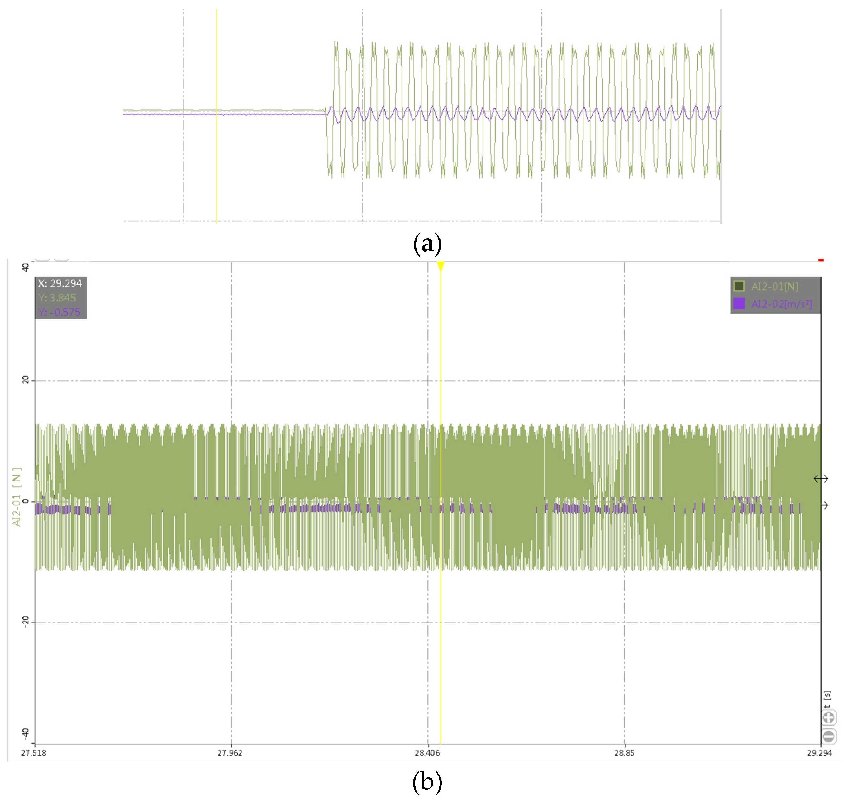
3.3. Ice Layer Excitation Experiment

Based on the results of the natural frequency experiment and numerical analysis of the ice layer, the exciter available in the laboratory was capable of reaching the 1st × 1st natural frequency of the ice layer. Therefore, an excitation experiment could be conducted to explore the effectiveness of resonance ice-breaking. The experimental setup for the ice layer excitation is shown in Figure 8 and Figure 9. In this setup, (a) and (b) were the same as those in the natural frequency experiment of the ice layer, namely the accelerometer and the low-temperature base; (c) was the exciter placed in the space suspended by four bases at the center below the ice layer, which was connected to the force sensor and the cruciform resin excitation head (d) before the experiment to provide the excitation load; (d) was the cruciform resin excitation head, which consisted of a metal rod and a cruciform resin head. A design using a low-modulus resin excitation head can effectively reduce the penetration effect between the excitation head and the ice body during the excitation process, allowing the excitation head to continuously transmit vibrations into the ice layer instead of penetrating a cavity within the ice layer in a short time.

When preparing the ice layer for the excitation experiment, the freezing steps had to be adjusted to freeze the excitation head together with the ice layer. After slowly pouring the solution into the mold, the cruciform resin excitation head designed for this experiment was placed upside down at the bottom of the mold. The mold was then placed into the ice-making machine for freezing after standing still to remove bubbles, with the remaining steps being the same. Similar to the natural frequency experiment, two hours before the experiment, the sensor base was placed into the ice-making machine to cool down and was frozen and bonded to the surface of the ice layer.

Before the experiment began, the ice layer was taken out of the ice-making machine along with the excitation head and sensor base. The excitation head, oriented downward, was connected to the exciter below the ice layer and was then placed steadily on the low-temperature base. The accelerometer was installed and connected to the DHDAS dynamic signal acquisition and analysis system, with the exciter connected to an oscilloscope. During the experiment, the exciter generated vibration signals, and the accelerometer monitored the vibration of the ice layer during the process to detect the occurrence of beat phenomena.

The experiment began with the measured 1st × 1st modal frequency of the ice layer being 257.798 Hz. Initially, a frequency sweep signal ranging from 200 Hz to 400 Hz was applied to the ice layer to identify its true natural frequency under excitation load by monitoring the trend of acceleration data. The instantaneous frequency when the acceleration reached its peak was approximately 258 Hz. Subsequently, the excitation frequency was fixed at 258 Hz, and the ice layer was continuously subjected to the excitation load. After about 20 s, the load and acceleration graphs of the ice layer displayed typical beat patterns, as shown in Figure 10. Meanwhile, the ice layer exhibited significant vibration, and the sound emitted by the excitation underwent a noticeable change. When the beat phenomenon persisted for about 90 s, the ice plate emitted a slight cracking sound. At this point, the load and acceleration graphs no longer showed beat patterns, and the excitation sound no longer possessed the characteristics of beat occurrence, indicating that the beat phenomenon had ceased.

After stopping the excitation, the ice layer was observed and slight, barely visible cracks were found near the excitation head. A small amount of red dye was dropped at the excitation head, and the dye spread along the slight cracks, revealing their presence, as shown in Figure 11, with the cracks radiating from the center of the excitation head. It was observed that the dye stopped spreading due to freezing, indicating that the temperature of the ice layer was still low. It can be inferred that after the cracks appeared, the small size of the cracks and the low ambient temperature might have caused the cracks to refreeze. Therefore, the area of slight cracks produced by the excitation may be larger than the dyed area shown in Figure 9. In summary, under the excitation load, the ice layer exhibited significant resonance beat vibration and radial cracks.

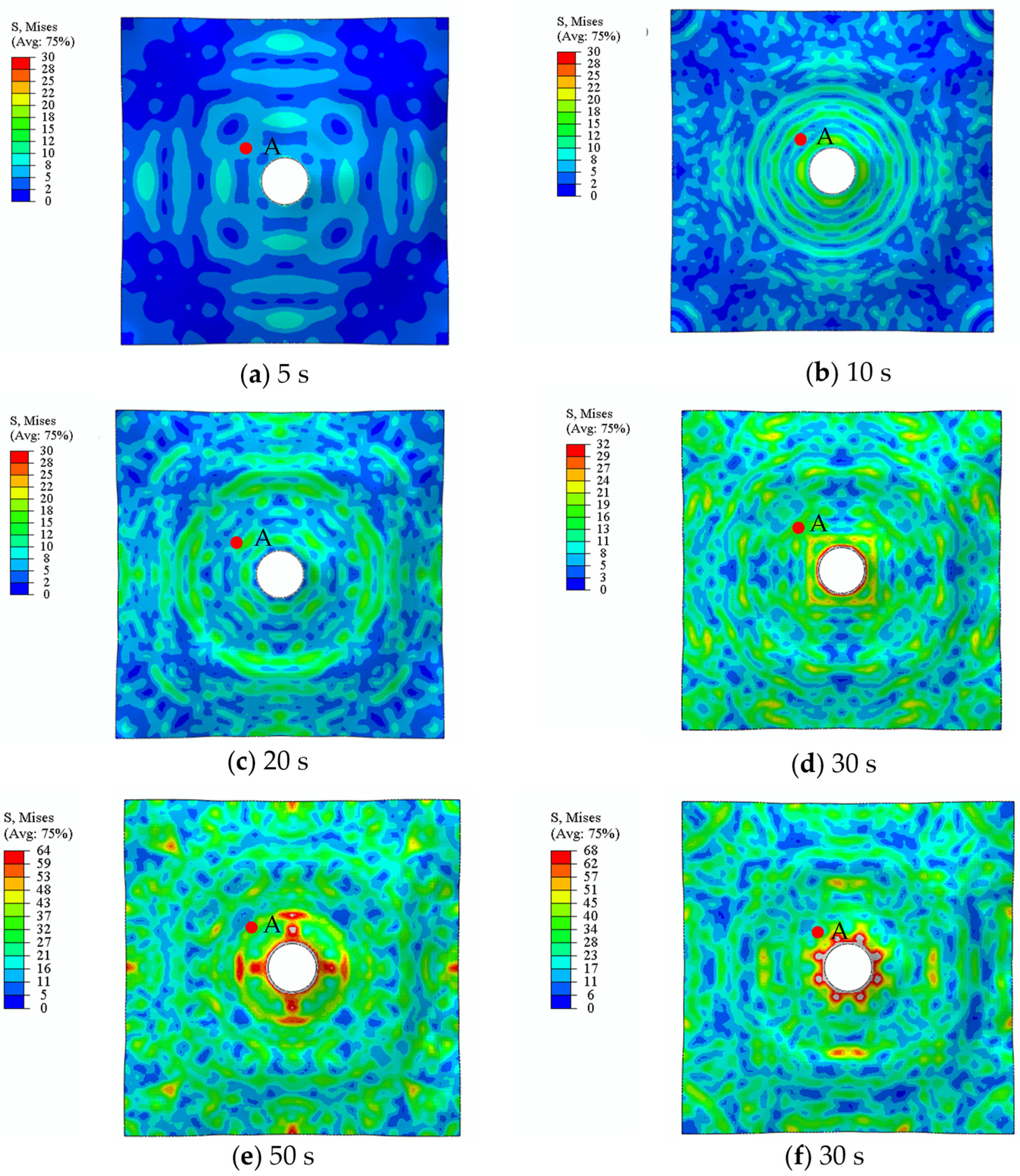
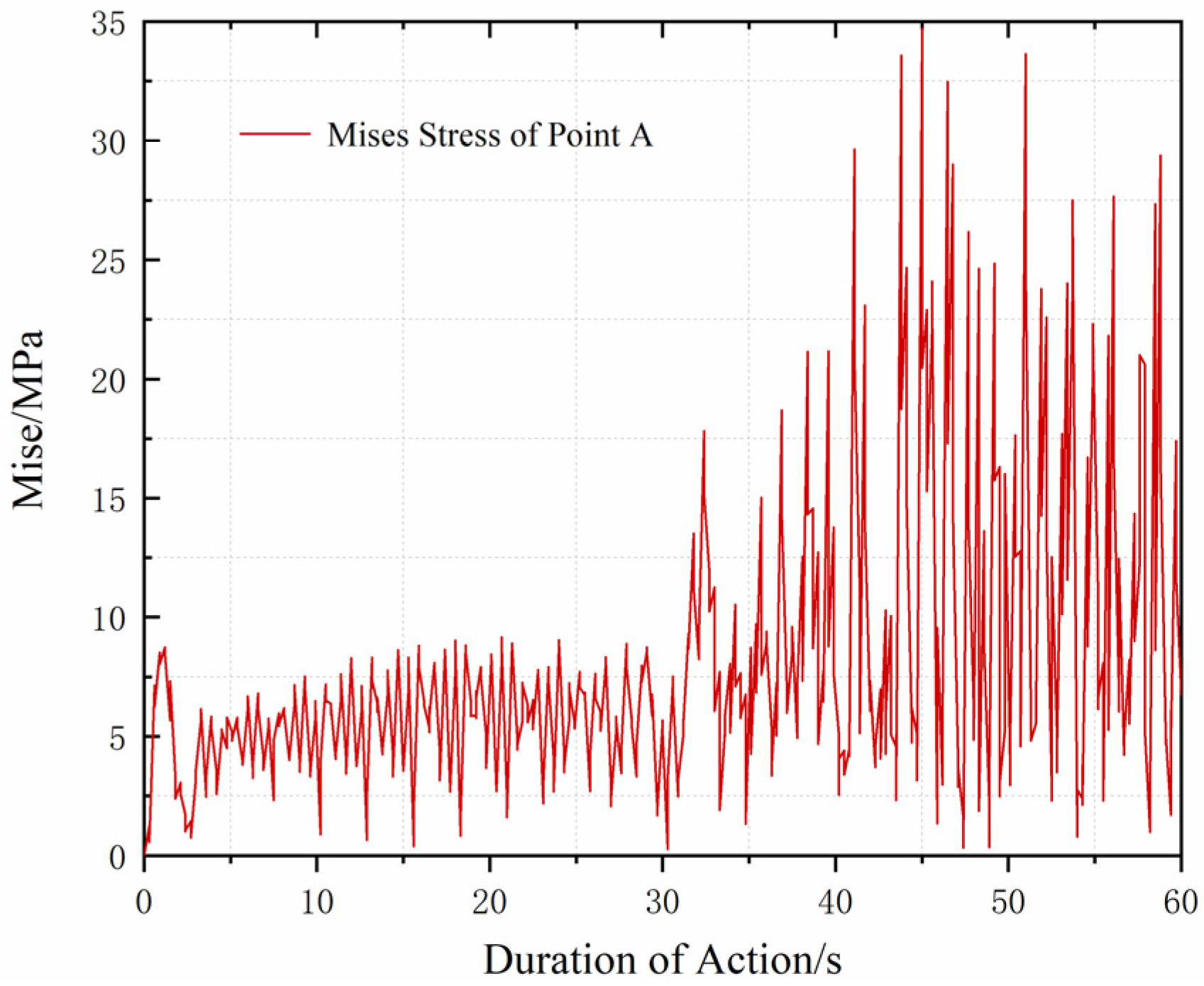
3.4. Numerical Simulation Analysis of Ice Layer Excitation Response

Given the complexity of the constitutive model of ice material, it is quite challenging to simulate the cracking and crack propagation in its complex deformation under excitation using numerical methods. Therefore, this study has employed dynamic simulation to investigate the stress distribution in the ice layer during the deformation response under excitation. If the Mises stress values in certain areas of the ice layer significantly exceed the material’s strength limit, it is considered that the ice layer model is highly likely to fracture under the excitation load.

In dynamic simulation, directly applying the excitation load to the ice layer model does not reflect the vibration characteristics of the model. Instead, it merely causes the model to be repeatedly pulled back and forth near the load point without generating vibrations. To induce vibrations in the dynamic model, the grid displacement matrix of the 1st × 1st vibration mode of the ice layer model, obtained from modal numerical analysis, is multiplied by 0.05 and used as the initial grid perturbation for the vibration dynamic simulation. The ice layer dynamic simulation model established by this method can accurately simulate the beating vibration phenomenon of the ice layer model under excitation at the 1st × 1st natural frequency, following the vibration mode of that order. The harmonic excitation concentrated force load of the sinusoidal periodic function is applied at the center of Region 2 in Figure 3a according to Equation (6).

$$F\left(t\right)=F_a\sin \omega t$$

(8)

Here, $F_a$ represents the amplitude of the excitation force, and $\omega$ (rad/s) is the excitation frequency set to the natural frequency of the ice layer. The frequency $\omega$ was set to 252.798 Hz, and the force amplitude $F_a$ was set to 100 N, with the excitation applied at the center of the ice layer. The Mises stress contour maps of the ice layer within 60 s are shown in Figure 12a–f. Due to the modeling issues with the load application in finite element simulation, stress concentration is more pronounced in the vicinity of the load point when a concentrated force is applied. To make the stress distribution in the non-concentrated stress regions more evident, the mesh within a radius of 1.5 mm around the load application point, where stress concentration occurs, was removed when analyzing the response stress contour maps of the ice layer. As seen in Figure 12a–f, as the excitation time increased, the stress response region caused by the vibration gradually expanded, and the proportion of high-stress areas within the model also increased. After the excitation time reached 60 s, the stress state of the model changed periodically and no longer continued to develop. It can be observed from the figures that 20 s after the start of excitation, some areas already exhibited stress levels of 15 MPa. At 20 s, the high-stress region began to extend to the edge of the model. By 30 s, the high-stress region accounted for about 90% of the model area, and at 60 s, the high-stress region still occupied about 90% of the model area, with the maximum stress reaching 67 MPa, which was significantly higher than the strength limit of the ice material.

A point A, located 3 mm from the center and at a 45° angle from the horizontal, as shown in Figure 12a–f, was selected on the model. The displacement and stress variation curves of point A over 60 s are shown in Figure 13. It can be observed that the stress at point A began to increase significantly at 30 s due to resonance, and the stress gradually stabilized after 45 s. According to the team’s previous research, the strength limit of the ice layer material is 1.8 MPa, and the stress required for the ice layer to fracture is within 12 MPa. At 45 s, the ultimate stress of the ice layer had already far exceeded the stress required for fracture.

4. Conclusions and Future Work

This study has proposed a method of ice-breaking by generating resonance through excitation to crack the ice layer. The vibration modes and natural frequencies of the ice layer were investigated using numerical simulation and experiments. Based on these findings, ice layer excitation experiments and numerical simulation analyses of the ice layer’s excitation response were conducted, leading to the following conclusions:

(1)

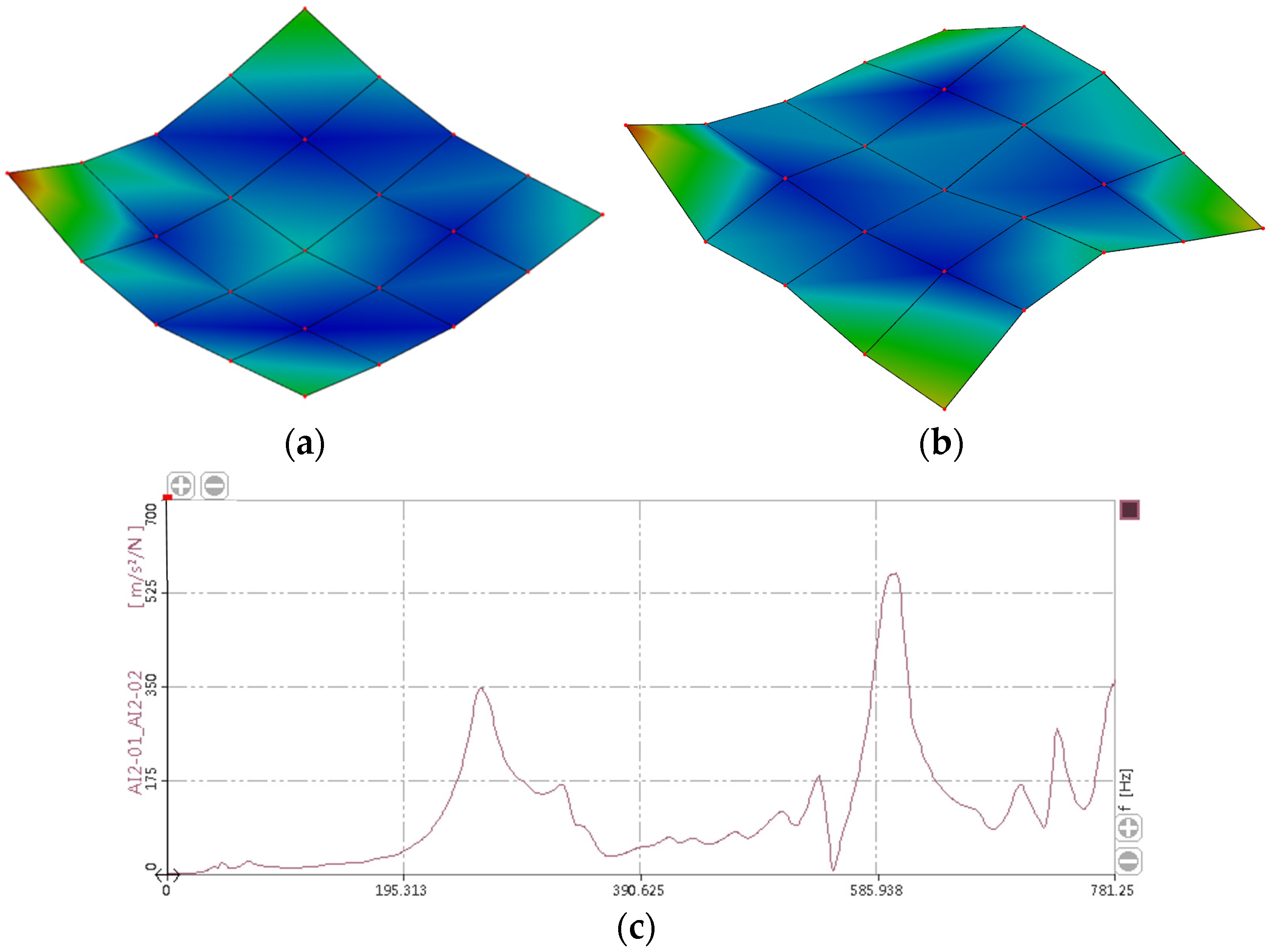
A comparison between the ice layer vibration mode analysis results based on the Abaqus software and the experimental modal results obtained from the ice layer impact test revealed that the error in the Ω₁ was 0.53%, while the error in the second-order modal simulation was 14.937%. Since the 1 × 1 order modal was used in the simulation, which has a lower error, this simulation method can accurately simulate the vibration modes and frequencies of the ice layer.

(2)

Based on Conclusion (1), for ice materials with unknown moduli, the actual modes and frequencies of ice specimens can be determined using the impact method. The modulus of the ice material can then be accurately calculated in reverse using the aforementioned simulation method.

(3)

The results of the ice layer excitation experiments and numerical simulation analysis of the ice layer’s excitation response indicate that resonance occurring in the ice layer under the excitation load is sufficient to generate stresses that reach the strength limit of the ice material over a large area and produce cracks.

This study has certain limitations:

(1)

Although a low-modulus resin excitation head was used in the excitation experiment, the head still penetrated and created cavities in the ice layer during the experiment. This caused the excitation load to be unable to continuously and stably transmit to the ice layer after cracks appeared, preventing the ice layer from fracturing and resulting in less pronounced experimental effects. Additionally, due to the limitations of the laboratory exciter, it is difficult to induce beat phenomena in thicker ice layers, so only thinner ice layers were studied. Future research will address these two issues by improving the experimental scheme and expanding the scope of the study.

(2)

Since this study only focused on thinner ice layers, shell elements were used for the finite element analysis when exploring the mechanism of resonance ice-breaking through numerical simulation. When the research object expands from thin ice plates to thicker ice layers, solid elements should be used for simulation, and appropriate constitutive relationships for the ice material should be selected to simulate the fracturing of the ice layer under the excitation load through finite element simulation. Moreover, the loading method of the excitation load in numerical simulation should be improved to avoid stress concentration, which could affect the analysis.

In summary, this study has essentially validated the feasibility of resonance ice-breaking. However, the dynamic response behavior of the ice material and the fracturing mechanism during resonance ice-breaking require further in-depth research. In particular, how to continuously and stably apply the excitation load sufficiently to induce beat phenomena in the ice layer will be a challenging issue for further experimental and numerical simulation research.

References

1. Ye, L.; Wang, C.; Guo, C.; Chang, X. Peri dynamic model for submarine surfacing through ice. Chin. J. Ship Res. 2018, 13, 51–59. [Google Scholar] [CrossRef]
2. Bai, T.C.; Xu, J.; Wang, G.D.; Yu, K.; Hu, X. Analysis of resistance and flow field of submarine sailing near the ice surface. Chin. J. Ship Res. 2021, 16, 36–48. [Google Scholar]
3. Engelbrektson, A. Observations of a resonance vibrating lighthouse structure in moving ice. In Proceedings of the Seventh POAC Conference, Helsinki, Finland, 5–9 April 1983; Volume 2, pp. 855–864. [Google Scholar]
4. Määttänen, M. Dynamic Ice-Structure Interaction During Continuous Crushing; US Army Corps of Engineers, Cold Regions Research & Engineering Laboratory: Hanover, NH, USA, 1983. [Google Scholar]
5. Tsuchiya, M.; Kanie, S.; Ikejiri, K.; Ikejiri, A.; Saeki, H. An experimental study on ice-structure interaction. In Proceedings of the Offshore Technology Conference. OTC, Houston, TX, USA, 6–9 May 1985; p. OTC-5055-MS. [Google Scholar]
6. Matlock, H.; Dawkins, W.P.; Panak, J. Analytical model for ice-structure interaction. J. Eng. Mech. Div. 1971, 97, 1083–1092. [Google Scholar] [CrossRef]
7. Shih, L.Y. Analysis of ice-induced vibrations on a flexible structure. Appl. Math. Model. 1991, 15, 632–638. [Google Scholar] [CrossRef]
8. Zhang, B.; Wang, Q.; Wang, T. Research on the deicing robot and motion characteristic of the four divisions high-voltage line. IOP Conf. Ser. Mater. Sci. Eng. 2018, 417, 012008. [Google Scholar] [CrossRef]
9. Kandagal, S.B.; Venkatraman, K. Piezo-actuated vibratory deicing of a flat plate. In Proceedings of the 46th AIAA/ASME/ASCE/AHS/ASC Structures, Structural Dynamics and Materials Conference, Austin, TX, USA, 18–21 April 2005; p. 2115. [Google Scholar]
10. Kong, X.; Guan, H.; Jiang, L.; Wang, Y.; Zhang, C. Icing detection on ADSS transmission optical fiber cable based on improved YOLOv8 network. Signal Image Video Process. 2024, 18, 5323–5332. [Google Scholar] [CrossRef]
11. He, X.; Ma, Y.; Wang, K.; Liu, C. The oretical study and simulation analysis of distributed vibration de-icing technology for medium voltage overhead lines. Appl. Math. Nonlinear Sci. 2025, 10, 1. [Google Scholar]
12. Xu, P.; Zhang, D.; Li, A. The de-icing method using synthesized envelope modulation signals from resonance low-frequency and ultrasonic signals. Appl. Acoust. 2025, 231, 110411. [Google Scholar] [CrossRef]
13. Dai, H.; Lang, J.; Pang, F.; Wang, Y. Research on Mechanism and Application of Ship Resonance Ice-Breaking. In Proceedings of the25th IAHR International Symposium on Ice, Dalian, China, 22–25 November 2020. [Google Scholar]
14. Bažant, Z.P.; Luo, W.; Chau, V.T.; Bessa, M.A. Wave dispersion and basic concepts of peridynamics compared to classical nonlocal damage models. J. Appl. Mech. 2016, 83, 111004. [Google Scholar] [CrossRef]
15. Kirane, K.; Su, Y.; Bažant, Z.P. Strain-rate-dependent microplane model for high-rate comminution of concrete under impact based on kinetic energy release theory. Proc. R. Soc. A Math. Phys. Eng. Sci. 2015, 471, 20150535. [Google Scholar] [CrossRef]
16. Shi, D.; Wang, Q.; Shi, X.; Pang, F. Free vibration analysis of moderately thick rectangular plates with variable thickness and arbitrary boundary conditions. Shock Vib. 2014, 2014, 572395. [Google Scholar] [CrossRef]
17. Du, Y.; Tang, Y.; Pang, F.; Ma, Y.; Zou, Y. A Semi-Analytical Method to Design Distributed Dynamic Vibration Absorber of Beam Under General Elastic Edge Constraints. Int. J. Struct. Stab. Dyn. 2024, 24, 2450181. [Google Scholar] [CrossRef]
18. Chai, W.; Leira, B.J.; Høyland, K.V.; Sinsabvarodom, C.; Yu, Z. Statis-tics of thickness and strength of first-year ice along the Northern Sea Route. J. Mar. Sci. Technol. 2021, 26, 331–343. [Google Scholar] [CrossRef]
19. Lv, X.; Shi, D. Free vibration of arbitrary-shaped laminated triangular thin plates with elastic boundary conditions. Results Phys. 2018, 11, 523–533. [Google Scholar] [CrossRef]
20. Xue, Y.; Liu, R.; Li, Z.; Han, D. A review for numerical simulation methods of ship–ice interaction. Ocean. Eng. 2020, 215, 107853. [Google Scholar] [CrossRef]
21. Cui, W.; Kong, D.; Sun, T.; Yan, G. Coupling dynamic characteristics of high-speed water-entry projectile and ice sheet. Ocean. Eng. 2023, 275, 114090. [Google Scholar] [CrossRef]
22. Song, Z.; Chen, R.; Guo, D.; Yu, C. Experimental investigation of dynamic shear mechanical properties and failure criterion of ice at high strain rates. Int. J. Impact Eng. 2022, 166, 104254. [Google Scholar] [CrossRef]
23. Dönmez, A.; Bažant, Z.P. Size effect on punching strength of reinforced concrete slabs with and without shear reinforcement. ACI Struct. J. 2017, 114, 875. [Google Scholar] [CrossRef]
Figure 1. Schematic diagram of the resonance ice-breaking process.
Jmse 13 01147 g001
Figure 2. Simplified system for central ice-layer vibration.
Jmse 13 01147 g002
Figure 3. (a) Schematic diagram of regional division. (b) Numerical simulation mesh diagram.
Jmse 13 01147 g003
Figure 4. Typical vibration modes of the ice layer plane. (a) 1st × 1st mode at 259.18 Hz. (b) 1st × 2nd mode at 393.50 Hz. (c) 2nd × 2nd mode at 419.04 Hz.
Jmse 13 01147 g004
Figure 5. Experimental setup for ice layer natural frequency testing.
Jmse 13 01147 g005
Figure 6. Schematic diagram of the experimental setup for ice layer natural frequency testing.
Jmse 13 01147 g006
Figure 7. Measurement results from the dynamic signal acquisition and analysis system: (a) 1st × 1st mode shape; (b) 1st × 2nd mode shape; (c) frequency response results.
Jmse 13 01147 g007
Figure 8. Ice layer excitation experimental setup.
Jmse 13 01147 g008
Figure 9. Schematic diagram of the ice layer excitation experimental setup.
Jmse 13 01147 g009
Figure 10. Load and acceleration curves of the ice layer during the beat phenomenon (where (a) is the curve recorded at the onset of the beat phenomenon, and (b) is the stabilized beat phenomenon. Among them, the green curve (AI2-01) is the applied load curve, with the unit of N; The purple curve (AI2-02) represents the measured acceleration of the ice).
Jmse 13 01147 g010
Figure 11. Photograph of the dyed crack area around the excitation head.
Jmse 13 01147 g011
Figure 12. Stress contour maps of the ice layer under excitation loads from dynamic numerical simulation.
Jmse 13 01147 g012
Figure 13. Time-varying curves of displacement and stress at the monitoring point on the ice layer.
Jmse 13 01147 g013