Research on Ship Engine Fuel Consumption Prediction Algorithm Based on Adaptive Optimization Generative Network

Abstract

With the long-term operation of ships, the performance of marine diesel engines gradually declines due to the wear of internal moving components, increasing the risk of potential failures. Fuel consumption is a critical indicator for assessing engine operating conditions, and accurately predicting baseline fuel consumption under normal operating conditions is essential for evaluating ship energy efficiency and conducting fault diagnosis. To address common issues in marine engine operational data, such as noise pollution, missing values, inconsistent scales, and feature redundancy, a Diesel Engine Data Enhancement and Optimization Framework (DEOF) was developed to systematically improve data quality. Furthermore, to overcome the limitations of existing models, such as insufficient prediction accuracy and poor stability under complex operating conditions, a Meta-learning Diffusion Residual Attention Network (MD-RAN) is proposed. This approach leverages the strengths of diffusion models in nonlinear generative modeling, integrates meta-learning mechanisms to enhance task adaptation speed, employs multi-head attention modules to strengthen feature extraction, and incorporates dynamic residual connections to improve training stability and flexibility. The data used in this study were collected from real-world operations of ocean-going vessels, ensuring high representativeness. This paper systematically benchmarks the proposed model with the traditional learning model. The results are verified to be effective. The MD-RAN algorithm is significantly better than the original model in terms of prediction accuracy, stability, and nonlinear expression ability. The R² value can reach 0.9853, and the RMSE and MAE are as low as 1.5801 and 1.1879, respectively. Its feasibility will be further evaluated in practical applications in the future. This study not only provides a systematic data-driven modeling framework, offering technical insights for constructing high-quality datasets, but also establishes a novel generative modeling approach for marine diesel engine fuel consumption prediction, providing robust support for intelligent engine maintenance and energy efficiency optimization.

1. Introduction

Ship diesel engines, with advantages such as high thermal efficiency and high power density, dominate the main propulsion power units of ships. Their operational reliability not only affects performance and economy but also impacts navigational safety and market competitiveness. The development and utilization of ship engine condition monitoring and fault diagnosis technologies are essential approaches for improving engine reliability. In the study [1], condition monitoring was performed using measured indicator diagrams and the thermodynamic parameters of the engine. In addition, a fuel consumption prediction method was employed for condition identification. The principle of this method is based on comparing the actual fuel consumption with the predicted fuel consumption. A significantly higher predicted fuel consumption indicates that a fault is likely to occur within the predicted period.

Currently, diesel engines, as the core of ship propulsion systems, directly impact vessel energy efficiency and safety. To enhance the accuracy and real-time performance of fault detection, various methods have been proposed in academia. From early methods that relied on feature engineering such as RCMFE and FASVM [2] and relied on thermal economic analysis [3] to the introduction of digital twin systems [4]; although the diagnostic completeness and theoretical depth have been enhanced, there are still problems such as complex deployment or insufficient positioning accuracy. Some review studies [5] provide valuable references for future development but lack systematic comparisons of emerging deep learning methods. In recent years, deep learning has become the mainstream trend in fault identification research. For instance, the Multi-Attention Convolutional Neural Network (MACNN) [6] excels in recognition accuracy, though its adaptability remains unverified. Infrared thermography combined with CNN techniques [7] achieves efficient identification but is heavily influenced by external conditions. One-dimensional CNNs with domain adaptation methods [8] enhance cross-condition robustness yet suffer from high computational complexity and limited real-time performance. Models integrating Temporal Convolutional Networks (TCNs) with attention mechanisms [9], multi-branch CNN structures [10], hybrid methods combining signal decomposition with fuzzy clustering [11], and improved thermodynamic diagnostic methods incorporating component condition characteristic curves [12] have also made breakthroughs in accuracy, stability, and feature extraction. However, these methods still face challenges such as low automation, high training dependency, and system complexity.

In summary, current mainstream methods often rely on complex sensor data and high-dimensional signal processing, posing significant demands on deployment and real-time performance. In contrast, fault diagnosis based on fuel consumption baseline modeling offers advantages due to its straightforward data acquisition, intuitive diagnostic logic, and deployment-friendly nature. By analyzing deviations in fuel consumption, overall engine performance changes can be monitored in real time, facilitating efficient intelligent maintenance. Therefore, fault identification methods based on fuel consumption prediction not only broaden traditional diagnostic approaches but also provide new perspectives for enhancing vessel operational safety and energy efficiency. This study focuses on this direction, aiming to explore novel intelligent diagnostic solutions with higher adaptability, accuracy, and robustness to address gaps in existing engineering applications.

In recent years, ship fuel consumption prediction has become a research hotspot in the maritime industry, aiming to improve operational efficiency and reduce energy waste. Numerous scholars have adopted various models and methods, incorporating external ship parameters for fuel prediction. Many studies focus on fuel consumption prediction under marine conditions to support speed optimization and other objectives. Ref. [13] proposed an adaptive intelligent learning network that captures latent evolutionary features during population iterations, enabling efficient targeted optimization for individuals. Ref. [14] designed a multi-objective optimization algorithm for optimal route planning for safe transoceanic voyages under complex sea conditions. Ref. [15] developed a novel multi-step load forecasting system capable of accurate load prediction on extremely short time scales (milliseconds).

Concurrently, with advancements in artificial intelligence and data-driven methods, ship fuel consumption modeling and operational condition analysis have become more refined. Increasingly, studies combine statistical methods with machine learning and deep learning models to enhance fuel prediction accuracy. Ref. [16] integrated an ANN with regression techniques to build ship performance models adaptable to different operating conditions, achieving more precise fuel predictions. Ref. [17] utilized passenger ship operational data for fuel consumption modeling, employing statistical methods and domain knowledge to select input variables, including multiple linear regression, decision trees, artificial neural networks, and ensemble methods, ultimately finding XGBoost to perform best. Ref. [18] combined shallow and deep learning methods to explore day-ahead fuel consumption prediction for passenger ships, addressing the scarcity of deep learning research in this domain. Ref. [19] applied five machine learning methods—linear regression, decision trees, random forests, XGBoost, and AdaBoost—for ship fuel consumption modeling, achieving high prediction accuracy. Ref. [20] used a Broad Learning System (BLS) alongside various time-series and machine learning models for fuel consumption prediction, but existing studies still lack comprehensive consideration of environmental factors, limiting model generalizability and accuracy. Ref. [21] employed EEMD-LSTM and BiLSTM for the multi-step fuel consumption prediction of marine diesel engines, improving accuracy for short-term fluctuations and long-term trends; however, existing methods lack their wide application in practical maintenance. Ref. [22] conducted a bibliometric analysis using CiteSpace on specific fuel consumption (SFC) models, systematically reviewing the types, applicability, and improvement directions of white-box, black-box, and gray-box models, providing a theoretical foundation and methodological reference for ship energy efficiency optimization and carbon emission prediction. Ref. [23] developed ship voyage fuel consumption prediction models using Huber regression and LGBM, focusing primarily on model performance comparisons. Ref. [24] constructed a ship fuel prediction and optimization model for specific transport systems using XGBoost and particle swarm optimization, though its generalizability requires further exploration. Ref. [25] built a Double Hidden Layer BP Neural Network (DBPNN) model based on multi-source sensor data to predict inland ship fuel consumption, but its adaptability to different route segments and environmental changes needs further study. Ref. [26] analyzed the ability of artificial neural networks to predict ship speed and fuel consumption using only sea condition information as the input, without considering engine condition data.

In summary, it can be seen that existing research has achieved certain results in ship fuel consumption prediction methods, covering a variety of modeling methods from traditional statistical regression to ensemble learning, deep learning, etc., and continuously expanding the integration of environmental variables, operating status, and sensor data. However, current methods face several limitations, primarily due to their reliance on the distributional characteristics of training data. Under complex operating conditions, fuel performance is influenced by multiple nonlinear factors, making it challenging for models to accurately adapt to these dynamic changes. Additionally, data-driven methods often overlook dynamic model adjustment capabilities, leading to reduced prediction accuracy in new conditions or unknown environments. As for the complex data of diesel engines, the lack of a unified and efficient data processing framework is also one of the problems present in current research. Therefore, it is necessary to further explore fuel consumption prediction models with greater robustness, adaptability, and accuracy to provide a more solid technical foundation for achieving smart shipping and green shipping goals.

This study addresses common issues in marine engine operational data, such as noise pollution, missing values, and anomalies, by proposing a systematic Data Enhancement and Optimization Framework (DEOF). Through multi-scale noise modeling and dynamic scale regularization mechanisms, DEOF ensures data integrity while significantly enhancing the stability and expressiveness of data distributions, thereby improving the robustness of the modeling foundation. Building on this, we further propose a Meta-optimized Diffusion Residual Attention Network (MD-RAN), incorporating multiple improvements in model architecture and training strategies to enhance modeling capabilities for complex nonlinear features. First, MD-RAN introduces a diffusion modeling module to simulate the continuous propagation of features within the network, effectively overcoming the limitations of traditional convolutions’ local receptive fields and enhancing the model’s ability to capture long-range feature dependencies. Additionally, the model incorporates a multi-head attention mechanism to capture multidimensional information in parallel from inputs, extracting key features from multiple perspectives and improving host feature identification under complex conditions. The dynamic residual connection mechanism adapts residual paths based on training state changes, optimizing gradient propagation efficiency and significantly enhancing training stability and convergence speed. Moreover, MD-RAN employs a meta-learning strategy at the optimization level, dynamically adjusting the learning process during training to improve adaptability to different data distributions or operating conditions, thereby accelerating convergence for new tasks. Through dual improvements in structure and optimization, MD-RAN effectively addresses challenges in nonlinear modeling, feature extraction, and training stability, providing robust support for enhancing the accuracy and efficiency of diesel engine fault diagnosis. Although the application of diffusion models and meta-learning in ship fuel consumption baseline prediction is an emerging research direction, related studies have validated their theoretical feasibility and adaptability. For instance, meta-learning has been successfully applied to small target recognition and FPSO vessel motion modeling in complex marine environments, demonstrating potential in handling data distribution changes and dynamic modeling tasks [27,28]. The diffusion model also shows excellent modeling ability in prediction tasks, such as weather forecasting and electric vehicle load prediction [29,30,31]. These cross-domain results provide a solid foundation for applying the proposed methods to ship fuel consumption prediction. Therefore, this study achieves synergistic innovation in data processing and model design, offering a theoretically grounded and practically feasible new pathway for high-precision fuel consumption modeling in complex maritime systems.

2. Methodology

2.1. Overall Framework

Marine diesel engines are widely used in the shipping and military industries. Their fuel consumption not only directly impacts economic efficiency and energy management but also serves as a crucial indicator for monitoring the operating conditions of the engine and detecting potential faults. Although the traditional fuel consumption prediction method based on engine thermodynamic characteristics and empirical formula has a certain physical explanation, it is difficult to accurately describe the complex nonlinear dynamic process of diesel engines. On the other hand, data-driven methods, such as Random Forest and Support Vector Machines, can accommodate the nonlinear nature of the data. However, they have limited feature capture capabilities under complex operating conditions and lack fine-tuning data processing. To address these issues, this study proposes a diesel engine fuel consumption prediction model based on a meta-learning optimized diffusion residual attention network (MD-RAN), as shown in Figure 1.

During marine engine operation, the engine room monitoring system generates a vast amount of measurement data for assessing the operational status of the machinery. However, this data is often contaminated by noise, missing values, and outliers during the acquisition and transmission processes. If not properly addressed, such data imperfections can adversely affect subsequent data analysis, model prediction, and decision support. To tackle these challenges, this study proposes a systematic Data Enhancement and Optimization Framework (DEOF) tailored for marine engine operational data. By incorporating multi-scale noise modeling, feature flow reconstruction mechanisms, dynamic scale regularization, and redundant feature reduction strategies, DEOF significantly enhances the stationarity and structural characteristics of the data distribution while preserving the integrity of the original information representations. This framework not only increases data density and discriminative capability but also effectively suppresses non-ideal disturbances introduced during data collection, providing a unified and highly abstracted data flow foundation for downstream modeling tasks, and substantially improving the universality and robustness of models under varying operational conditions.

Aiming at the problems of nonlinear modeling difficulty, limited adaptive ability, weak feature focus, unstable training process, etc., in the intelligent ship engine fuel consumption prediction algorithm, a meta-learning optimized diffuse residual attention network (MD-RAN) is proposed. Anchored on the diffusion process as the modeling substrate, MD-RAN employs a meta-optimization paradigm to guide parameter updates and dynamically restructure the feature representation space, thereby substantially enhancing the model’s capacity to capture complex nonlinear relationships. The integration of multi-head attention mechanisms enables intricate coupling and interaction within and across feature dimensions, while the construction of dynamic residual flows adaptively adjusts the gradient propagation pathways, simultaneously improving training stability and generalization under diverse operating conditions. Through the synergistic interaction of multi-scale feature capture and meta-optimization feedback, the proposed architecture overcomes the performance bottlenecks encountered by conventional models in complex system modeling and establishes a novel generative modeling paradigm for diesel engine fuel consumption prediction. Consequently, a meta-learning optimized diffusion residual attention network is developed to achieve the high-precision prediction of marine engine fuel consumption, providing critical technical support for engineers to accurately assess the operational status of engines and to implement preventive maintenance strategies in a timely manner.

2.2. Diffusion Model

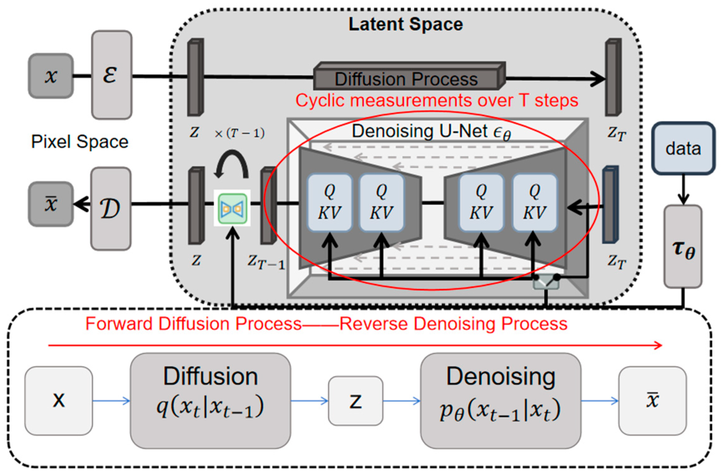
The diffusion model is a probabilistic deep learning technique widely applied in generative tasks and predictive modeling, such as image generation, data forecasting, and data recovery. Its core principle involves learning to reconstruct meaningful patterns from random noise by simulating a process of “noise addition” and “denoising”. In engineering applications, this model is particularly well-suited for handling complex, nonlinear data, such as the variables involved in ship fuel consumption prediction.

The working mechanism of diffusion models consists of two stages. as shown in Figure 2. First, controlled random noise is incrementally added to the original data, gradually transforming it into a standard Gaussian distribution. This process is predefined and straightforward to implement, typically controlled by a time-step schedule (e.g., linearly increasing noise). Second, starting from pure noise, a deep neural network iteratively removes noise to recover a distribution closely resembling the true data. This part requires the network to learn how to predict and correct noise at each step to generate samples that meet the target.

The diffusion model achieves data generation by leveraging the interplay between a forward process, which incrementally adds Gaussian noise to provide a reversible perturbation path, and a reverse process, where a neural network learns to denoise and capture the underlying data structure. This mechanism mimics physical diffusion processes to explore high-dimensional spaces and learn latent patterns. In the context of diesel engine fuel consumption prediction, this approach enables the model to capture complex nonlinear relationships and random perturbations among engine operating parameters, enhancing adaptability to anomalous data while generating smooth predictions that closely align with the true fuel consumption distribution. This not only improves prediction accuracy but also allows for modeling fuel consumption trends under varying operating conditions, supporting engine efficiency optimization and fuel management. Additionally, it mitigates the mode collapse issues common in traditional generative models, thereby enhancing robustness.

The forward diffusion is implemented through a Markov chain, transforming the real data distribution $\mathrm{q}({\mathrm{x}}_0)$ into a Gaussian noise distribution. The conditional distribution of a single step of diffusion is defined as follows:

$$\mathrm{q}({\mathrm{x}}_{\mathrm{t}}|{\mathrm{x}}_{\mathrm{t}-1})=\mathrm{N}({\mathrm{x}}_{\mathrm{t}};\sqrt{1-{\mathsf{\beta }}_{\mathrm{t}}}{\mathrm{x}}_{\mathrm{t}-1},{\mathsf{\beta }}_{\mathrm{t}}\mathrm{I})$$

(1)

where ${\mathrm{x}}_{\mathrm{t}}$ represents the data state at time step $\mathrm{t}$; ${\mathsf{\beta }}_{\mathrm{t}}$∈(0, 1) is the noise addition coefficient at time step t; and $\mathrm{N}$ is the Gaussian distribution.

Through multi-step recursion, the distribution at any time step $\mathrm{t}$ can be directly obtained:

$$\mathrm{q}({\mathrm{x}}_{\mathrm{t}}|{\mathrm{x}}_0)=\mathrm{N}({\mathrm{x}}_{\mathrm{t}};\sqrt{{\overline{\mathsf{\alpha }}}_{\mathrm{t}}}{\mathrm{x}}_0,(1-{\overline{\mathsf{\alpha }}}_{\mathrm{t}})\mathrm{I})$$

(2)

where ${\overline{\mathsf{\alpha }}}_{\mathrm{t}}={\prod }_{\mathrm{i}=1}^{\mathrm{t}}(1-{\mathsf{\beta }}_{\mathrm{i}})$ represents the cumulative noise intensity.

The reverse generation process attempts to reverse the noise added during the forward diffusion process. Its conditional distribution can be expressed as follows:

$${\mathrm{p}}_{\mathsf{\theta }}({\mathrm{x}}_{\mathrm{t}-1}|{\mathrm{x}}_{\mathrm{t}})=\mathrm{N}({\mathrm{x}}_{\mathrm{t}-1};{\mathsf{\mu }}_{\mathsf{\theta }}({\mathrm{x}}_{\mathrm{t}},\mathrm{t}),{\sum }_{\mathsf{\theta }}({\mathrm{x}}_{\mathrm{t}},\mathrm{t}))$$

(3)

where ${\mathsf{\mu }}_{\mathsf{\theta }}({\mathrm{x}}_{\mathrm{t}},\mathrm{t})$ represents the denoised mean learned by the neural network; ${\sum }_{\mathsf{\theta }}({\mathrm{x}}_{\mathrm{t}},\mathrm{t})$ is the denoised variance learned by the network; and $\mathsf{\theta }$ represents the parameters of the neural network. Through stepwise sampling, the model gradually generates the target data distribution from the initial noise.

The training objective of the diffusion model is to minimize the difference between the real distribution $\mathrm{q}({\mathrm{x}}_{\mathrm{t}}|{\mathrm{x}}_0)$ and the generated distribution ${\mathrm{p}}_{\mathsf{\theta }}({\mathrm{x}}_{\mathrm{t}-1}|{\mathrm{x}}_{\mathrm{t}})$. Through variational inference, the log-likelihood maximization problem is transformed into the optimization of the following loss function:

$$\mathrm{L}(\mathsf{\theta })={\mathrm{E}}_{{\mathrm{x}}_0,\mathsf{ϵ},\mathrm{t}}\left[{\Vert \mathsf{ϵ}-{\mathsf{ϵ}}_{\mathsf{\theta }}({\mathrm{x}}_{\mathrm{t}},\mathrm{t})\Vert }^2\right]$$

(4)

where $\mathsf{ϵ}~\mathrm{N}(0, 1)$ represents the normal distribution noise, and ${\mathsf{ϵ}}_{\mathsf{\theta }}({\mathrm{x}}_{\mathrm{t}},\mathrm{t})$ is the noise predicted by the model. This objective function directly corresponds to the noise prediction task, where the neural network learns the denoising mapping.

In practical applications, the acceptable difference between the true distribution and the generated distribution of a diffusion model can be evaluated using the R² metric. Through iterative sampling, the model progressively generates the target data distribution from initial noise. In the context of fuel consumption baseline prediction, an R² value greater than 0.8 is typically considered acceptable, though specific requirements should be further validated based on the application.

2.3. Meta-Learning Module

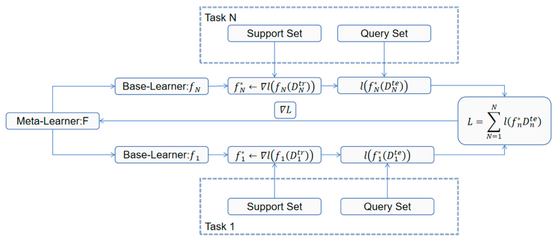
Meta-learning [32], commonly referred to as “learning to learn,” is a practical machine learning approach designed to accumulate experience through multi-task training, enabling models to quickly adapt and perform efficiently in scenarios with new tasks or limited data. In engineering applications, such as ship fuel consumption prediction or industrial equipment optimization, this method facilitates rapid adaptation to varying environmental conditions or equipment types. The working principle is shown in Figure 3. Its core lies in constructing a two-tier learning framework: the task layer and the meta-layer. The task layer focuses on training models for specific problems, optimizing parameters or rules to address the task at hand. In contrast, the meta-layer extracts commonalities across multiple tasks, deriving generalizable initialization settings, optimization strategies, or network architecture designs to provide a “shortcut” for new tasks.

Assume there exists a task distribution $\mathrm{p}(\mathrm{T})$ from which task sets $\{{\mathrm{T}}_1,{\mathrm{T}}_2,\dots ,{\mathrm{T}}_{\mathrm{N}}\}$ can be drawn for training. The goal is to enable the model to quickly adapt to future tasks ${\mathrm{T}}_{\mathrm{n}\mathrm{e}\mathrm{w}}$ sampled from the same distribution.

Task Level: Learn the optimal parameters for completing a single task. The task level focuses on local optimization for a specific task, where the model adjusts its parameters based on training data to achieve the best performance on that task.

Meta-Level: Learn meta-parameters or strategies across the task set to enable the model to rapidly adapt to new tasks. The meta-level focuses on discovering cross-task patterns by optimizing a meta-objective function, allowing the model to achieve optimal performance on new tasks with minimal training cost.

The objective of meta-learning is to enable the model to learn a new task after encountering only a small amount of new task data, using a few gradient updates or minimal computation. For a single task ${\mathrm{T}}_{\mathrm{i}}$, the model aims to find the optimal parameters ${\mathsf{\theta }}_{\mathrm{i}}$ that achieve the best performance on the task’s training data ${\mathrm{D}}_{\mathrm{i}}^{\mathrm{t}\mathrm{r}\mathrm{a}\mathrm{i}\mathrm{n}}$. The loss function at the task level is defined as follows:

$${\mathrm{L}}_{\mathrm{i}}^{\mathrm{t}\mathrm{r}\mathrm{a}\mathrm{i}\mathrm{n}}(\mathsf{\theta })={\displaystyle \frac{1}{|{\mathrm{D}}_{\mathrm{i}}^{\mathrm{t}\mathrm{r}\mathrm{a}\mathrm{i}\mathrm{n}}|}}\sum _{(\mathrm{x},\mathrm{y})\in {\mathrm{D}}_{\mathrm{i}}^{\mathrm{t}\mathrm{r}\mathrm{a}\mathrm{i}\mathrm{n}}}\mathrm{l}({\mathrm{f}}_{\mathsf{\theta }}(\mathrm{x}),\mathrm{y})$$

(5)

where $\mathrm{l}$ is the loss function for a specific task, and ${\mathrm{f}}_{\mathsf{\theta }}$ is the parameterized model.

By minimizing the task loss function ${\mathrm{L}}_{\mathrm{i}}^{\mathrm{t}\mathrm{r}\mathrm{a}\mathrm{i}\mathrm{n}}(\mathsf{\theta })$, the task-specific parameters are obtained:

$${\mathsf{\theta }}_{\mathrm{i}}={\mathrm{a}\mathrm{r}\mathrm{g}\mathrm{m}\mathrm{i}\mathrm{n}}_{\mathsf{\theta }}{\mathrm{L}}_{\mathrm{i}}^{\mathrm{t}\mathrm{r}\mathrm{a}\mathrm{i}\mathrm{n}}(\mathsf{\theta })$$

(6)

The objective of meta-level optimization is to learn a shared meta-parameter $\mathsf{\varphi }$ through training on multiple tasks, enabling it to provide better initialization, optimization rules, or model architecture for new tasks. The meta-level loss function is optimized based on the test set error of the tasks:

$${\mathrm{L}}^{\mathrm{m}\mathrm{e}\mathrm{t}\mathrm{a}}(\mathsf{\varphi })={\mathrm{E}}_{{\mathrm{T}}_{\mathrm{i}}~\mathrm{p}(\mathrm{T})}[{\mathrm{L}}_{\mathrm{i}}^{\mathrm{t}\mathrm{e}\mathrm{s}\mathrm{t}}({\mathsf{\theta }}_{\mathrm{i}}(\mathsf{\varphi }))]$$

(7)

where ${\mathrm{L}}_{\mathrm{i}}^{\mathrm{t}\mathrm{e}\mathrm{s}\mathrm{t}}$ is the error of task ${\mathrm{T}}_{\mathrm{i}}$ on the test data of task ${\mathrm{D}}_{\mathrm{i}}^{\mathrm{t}\mathrm{e}\mathrm{s}\mathrm{t}}$, and ${\mathsf{\theta }}_{\mathrm{i}}(\mathsf{\varphi })$ is the task-specific parameter optimized based on the meta-parameter $\mathsf{\varphi }$:

$${\mathsf{\theta }}_{\mathrm{i}}(\mathsf{\varphi })=\mathsf{\varphi }-\mathsf{\alpha }{\nabla }_{\mathsf{\varphi }}{\mathrm{L}}_{\mathrm{i}}^{\mathrm{t}\mathrm{r}\mathrm{a}\mathrm{i}\mathrm{n}}(\mathsf{\varphi })$$

(8)

where $\mathsf{\alpha }$ is the learning rate for the inner-level optimization.

By minimizing the meta-level loss function ${\mathrm{L}}^{\mathrm{m}\mathrm{e}\mathrm{t}\mathrm{a}}(\mathsf{\varphi })$, the meta-parameter $\mathsf{\varphi }$ is updated:

$$\mathsf{\varphi }=\mathsf{\varphi }-\mathsf{\beta }{\nabla }_{\mathsf{\varphi }}{\mathrm{L}}^{\mathrm{m}\mathrm{e}\mathrm{t}\mathrm{a}}(\mathsf{\varphi })$$

(9)

where $\mathsf{\beta }$ is the learning rate for meta-level optimization.

Meta-learning uses a two-layer optimization mechanism to learn the meta-parameter $\mathsf{\varphi }$, enabling the model to quickly adapt to new tasks. The network architecture is shown in Figure 4. The task level focuses on local learning for a single task, optimizing the task parameters ${\mathsf{\theta }}_{\mathrm{i}}$, while the meta-level focuses on global learning across tasks, improving the model’s generalization ability and adaptability by minimizing the meta-loss ${\mathrm{L}}^{\mathrm{m}\mathrm{e}\mathrm{t}\mathrm{a}}$.

On the above basis, combined with the characteristics of ship operation data, specific engineering configurations, including the number of network layers, activation functions, and number of cycles, were formulated. These configurations not only ensure that the model has good expressiveness but also fully consider the balance between computing resources and training efficiency and build an intelligent modeling framework that combines predictive performance with engineering practicality. The relevant configurations are shown in

Table 1. Engineering-level configuration of the main model.

Main Model Name	Engineering Level Configuration
diffusion model	Number of network layers = 3rd floor, hidden_dim = 128, Epoch = 300, activation function = ReLU, Dropout = 0.2
meta-learning	num_epochs = 300, num_tasks = 10, inner_lr = 0.01, outer_lr = 0.001, inner_steps = 1–5, batch_size = 32

:

2.4. Optimization Strategy

2.4.1. Dynamic Adjustment of Noise Level

In the diffusion model, a fixed noise level is used for perturbation during each training cycle. In practical applications, the intensity of the noise significantly affects the model’s convergence speed and robustness. Excessive noise can prevent the model from learning effectively, while insufficient noise can lead to overfitting. Therefore, in this optimization strategy, the noise level is dynamically adjusted, gradually decreasing as the training cycles progress. The specific formula is as follows:

$$\mathrm{n}\mathrm{o}\mathrm{i}\mathrm{s}\mathrm{e}\_\mathrm{l}\mathrm{e}\mathrm{v}\mathrm{e}\mathrm{l}=0.1\times (1-{\displaystyle \frac{\mathrm{e}\mathrm{p}\mathrm{o}\mathrm{c}\mathrm{h}}{\mathrm{n}\mathrm{u}\mathrm{m}\_\mathrm{e}\mathrm{p}\mathrm{o}\mathrm{c}\mathrm{h}\mathrm{s}}})$$

(10)

This dynamic adjustment strategy allows the model to quickly explore potential relationships in the data in the early stages, while gradually focusing on finer details of the data in the later stages, thereby improving training stability. In the early stages of training, a higher noise level helps prevent the model from becoming stuck in local optima, enabling the model to explore more data features. As training progresses, the noise level gradually decreases, aiding in the refinement of the model’s learning and gradually converging to a more precise solution.

2.4.2. Introduction of Multi-Head Self-Attention Mechanism

In the diffusion model, data is primarily processed through fully connected layers (FCs). However, when handling high-dimensional data and complex patterns, a single fully connected layer may not effectively capture the nonlinear relationships between data points. To address this issue, the optimization strategy introduces a multi-head self-attention mechanism, allowing the model to focus on the interrelationships between different parts of the input features, thereby enhancing the model’s ability to represent features.

The introduction of the multi-head self-attention mechanism enables the model to focus on different parts of the input data at each layer, learning the relationships between different parts. This helps capture long-range dependencies and complex patterns within the data. Additionally, it allows the model to learn different feature representations in multiple subspaces in parallel, thereby strengthening the model’s ability to capture potential correlations in the data. By allowing the model to learn information across multiple subspaces, the multi-head self-attention mechanism contributes to improved convergence speed and generalization ability.

Specifically, after the input data passes through the first fully connected layer (fc1), it is sent to the self-attention layer. Through the self-attention mechanism, the model assigns different attention weights to each input feature, enhancing its focus on different features. The formula is as follows:

$$\mathrm{A}\mathrm{t}\mathrm{t}\mathrm{e}\mathrm{n}\mathrm{t}\mathrm{i}\mathrm{o}\mathrm{n}(\mathrm{Q},\mathrm{K},\mathrm{V})=\mathrm{s}\mathrm{o}\mathrm{f}\mathrm{t}\mathrm{m}\mathrm{a}\mathrm{x}({\displaystyle \frac{\mathrm{Q}{\mathrm{K}}^{\mathrm{T}}}{\sqrt{{\mathrm{d}}_{\mathrm{k}}}}})\mathrm{V}$$

(11)

where $\mathrm{Q}$ is the query matrix, $\mathrm{K}$ is the key matrix, $\mathrm{V}$ is the value matrix, and ${\mathrm{d}}_{\mathrm{k}}$ is the dimension of the key. The multi-head attention mechanism enables the model to independently learn different feature representations in multiple subspaces, improving the expressiveness of the model.

2.4.3. Introduction of Dynamic Residual Connections

The original model may face the problem of vanishing gradients when dealing with deep networks. Therefore, dynamic residual connections are introduced, which help the model propagate gradients more effectively during training and accelerate convergence. The principle of residual connections lies in adding “shortcut connections” within the network, directly adding the input data to the output layer, and preventing information from gradually disappearing in deep networks.

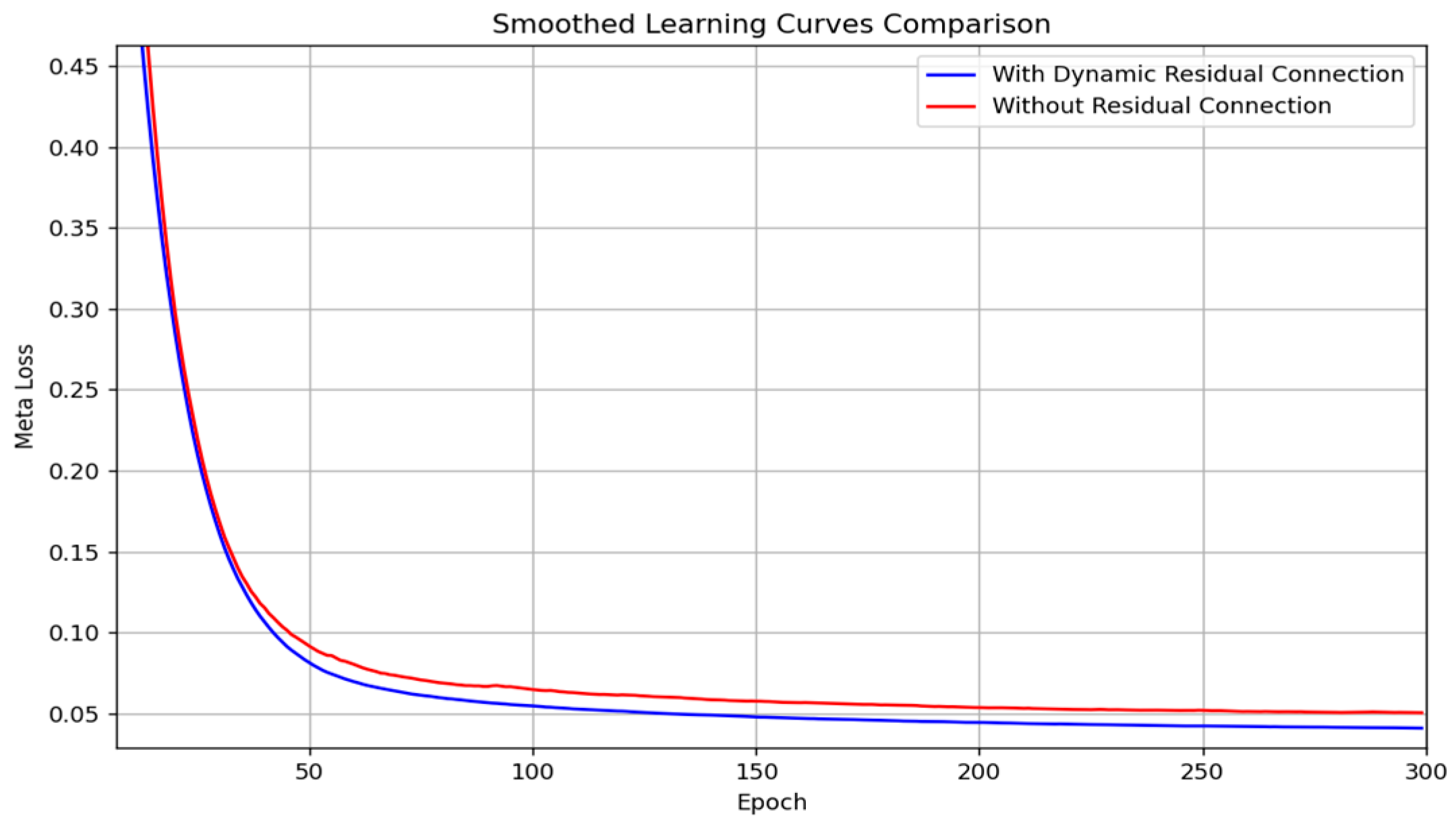
To further quantify the role of dynamic residual connections, we introduced a learnable parameter, residual_weight, and tracked its changes during the training process. As shown in Figure 5, this parameter gradually converges to a stable value (approximately 0.05), indicating that the model effectively dynamically integrates input information with intermediate features. We also compared the convergence speed of learning curves between models with and without residual connections. The former exhibited a faster decline in the first 100 epochs and required fewer training epochs to reach a specified error threshold. Additionally, from the perspective of error distribution, the model with residual connections demonstrated smaller errors on extreme predicted values, resulting in more stable predictions. These findings collectively confirm that dynamic residual connections effectively enhance model performance and convergence efficiency.

2.4.4. Meta-Learning Step Optimization

The basic framework of meta-learning typically uses a fixed number of inner-loop steps to perform task training, without dynamically adjusting the number of steps based on the validation set loss. Traditionally, the number of inner-loop steps in meta-learning is predetermined as a hyperparameter. However, a new mechanism has been proposed, where the number of inner-loop steps is dynamically adjusted according to the changes in the validation loss. The goal is to allocate training resources more flexibly and efficiently enable model adaptation. This strategy allows the model to dynamically adjust the training intensity according to the difficulty of the specific task and the learning progress, further improving the training efficiency of the model in complex scenarios.

The core objective of meta-learning is to enable a model to rapidly adapt to new tasks with minimal gradient updates or computational steps, even when provided with limited task-specific data. For a single task, the model learns optimal parameters by minimizing a task-specific loss function. Building on this, meta-learning trains across multiple tasks to learn shared meta-parameters, which provide better initialization, optimization strategies, or model architectures for future tasks. This process employs a two-tier optimization mechanism: the task layer focuses on local learning for individual tasks, optimizing task-specific parameters, while the meta-layer concentrates on global learning across tasks, minimizing a meta-loss function to enhance the model’s adaptability to new tasks.

During the training process, each inner loop randomly samples from the training set to construct a data subset for the current task and performs multiple rounds of iterative updates on the model parameters on this data. To enhance model robustness, Gaussian noise is applied to the input data during each step of the inner-loop training. After task training is completed, the model’s performance on that task is evaluated using a validation set. Notably, the outer loop dynamically adjusts the number of training steps in the inner loop based on changes in the validation loss:

$$\mathrm{inner}\_\mathrm{steps}=\left\{\begin{array}{c}\min (\mathrm{inner}\_\mathrm{steps}+1,10) \mathrm{if} \mathrm{validation} \mathrm{loss} \mathrm{decreases}\\ \max (\mathrm{inner}\_\mathrm{steps}-1,5) \mathrm{if} \mathrm{validation} \mathrm{loss} \mathrm{does} \mathrm{not} \mathrm{decreases}\end{array}\right.$$

(12)

Through this mechanism, the number of inner-loop steps can be adaptively adjusted based on changes in the validation loss, thereby improving training efficiency.

2.4.5. Task Selection Strategy

In the original algorithm, task selection is performed by randomly sampling a portion of the training data to construct tasks. While this method is effective, it does not fully leverage the diversity of the data and the relationships between tasks. In the optimized approach, task selection and inner-loop training are more refined. A task selection strategy is employed, where tasks are chosen and weighted according to their difficulty and the distribution of the data. This ensures the diversity and representativeness of the training data, thereby improving the distinguishability between tasks and the adaptability of the model.

Through the task selection strategy, each task during inner-loop training can represent different patterns or levels of difficulty in the data, enhancing the effectiveness of the training process. The optimized task selection method better balances the training weight between tasks, improving the model’s performance in multi-task learning.

3. Case Study

3.1. Data Description

The data used in this study were sourced from a bulk carrier operating on international routes, equipped with a two-stroke, low-speed, high-power marine diesel engine (Guangxi Yuchai Machinery Group Co., Ltd., Guangxi, China) (DMD-MAN B&W 5G60ME-C 10.5) using low-sulfur oil. The relevant parameters of the diesel engine are shown in

Table 2. Relevant technical parameters.

Diesel Engine Parameter Name	Parameter Value
Bore × Stroke (mm)	600 × 2250
Brake Mean Effective Pressure (BMEP)	10.5 bar
Maximum Continue Running (M.C.R)	8304 KW × 79.5 rpm
Minimum Continue Running (N.C.R)	6120 KW × 71.8 rpm
MAX CRITICAL RANGE	43–53 RPM
Fuel Consumption Rate	165–170 g/kWh
Fuel flexibility	HFO, LSFO, and MDO, with future-ready compatibility for carbon-neutral fuels

. The vessel was launched on 18 April 2023, with a ship age of two years. The research utilized measured operation data collected from September to December 2024 during voyages from Recife Port, Brazil, to Shanghai Port, China, spanning a total of five months and comprising 3,787 data points (Figure 6). Data were sampled at one-hour intervals, resulting in 24 time points per day, covering both steady-state and partial variable operating conditions to ensure the representativeness and diversity of the dataset.

It should be noted that the dataset excludes information on the vessel’s stationary state, and due to the short duration of the engine startup phase, fuel consumption variations during this phase were not separately captured. Additionally, given the relatively short data collection period, changes in the geometric compression ratio of the marine diesel engine were negligible and typically not monitored in the system; hence, this parameter was not included in the study.

The original dataset includes parameters such as scavenging pressure, scavenging temperature, exhaust manifold temperature, exhaust manifold pressure, main engine speed, turbocharger speed, turbocharger back pressure, engine load, engine fuel consumption, lubricating oil inlet temperature, engine room environment pressure, and engine room environment humidity. This study primarily focuses on the impact of the internal parameters of the diesel engine on the main engine’s fuel consumption.

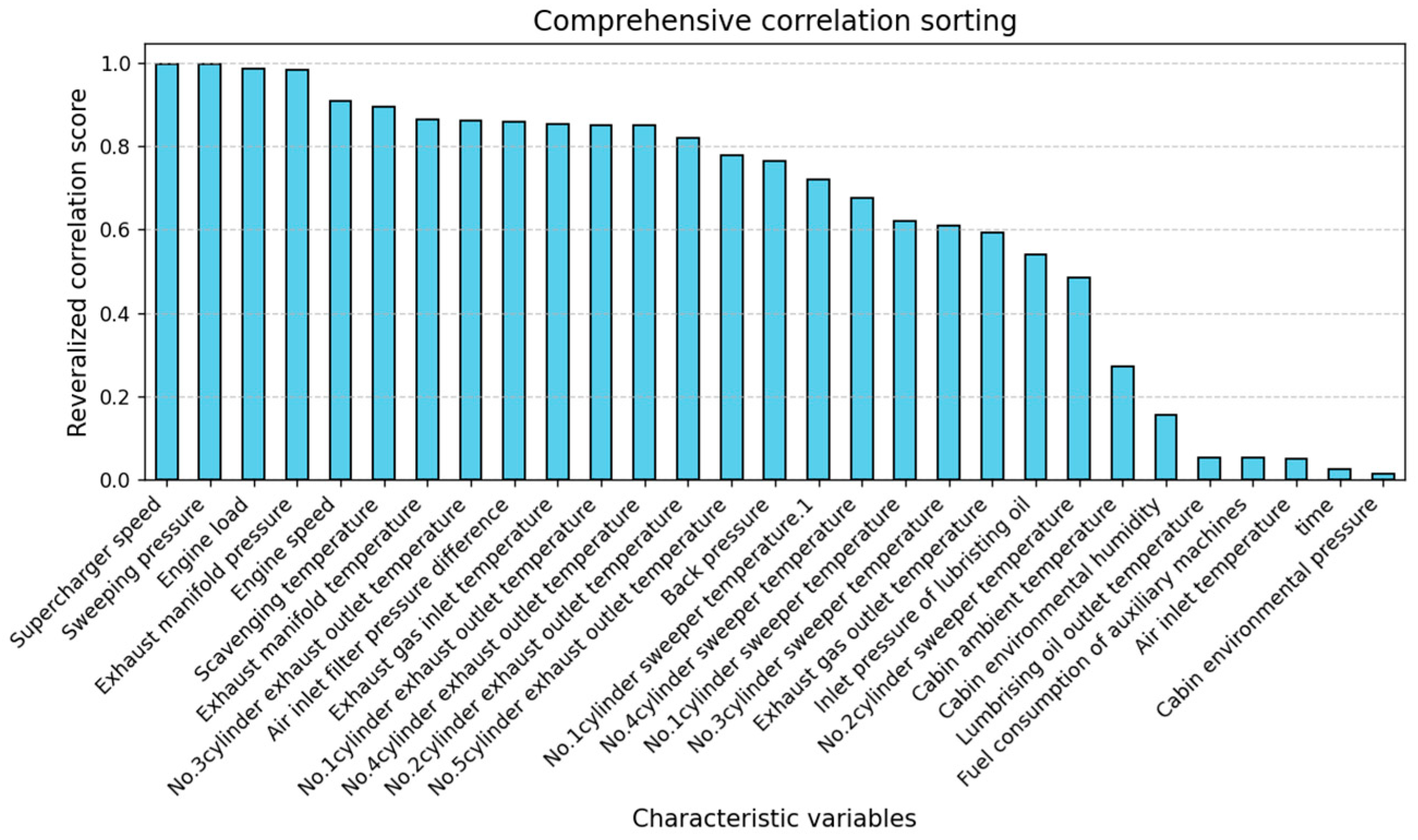
The dataset selected in this paper contains the operating parameters of relevant internal components of diesel engines. To measure the linear and nonlinear correlations between these features and the main engine fuel consumption, Pearson, Spearman, and Kendall correlation coefficients are used [33]. The Pearson correlation coefficient measures the linear relationship between two variables, with a range of [−1, 1]. The Spearman correlation coefficient measures the monotonic relationship between two variables, independent of linearity assumptions, making it suitable for nonlinear relationships. The Kendall correlation coefficient measures the consistency of rankings between variables, reflecting the relative order relationships between them. Figure 7 shows the comprehensive correlation sorting of all parameters.

Table 3. Correlation between different feature parameters and main engine fuel consumption.

Feature Name	Pearson	Spearman	Kendall
Supercharger speed	0.9891	0.9430	0.8212
Sweeping pressure	0.9779	0.9423	0.8277
Engine load	0.9907	0.9333	0.8008
Exhaust manifold pressure	0.9787	0.9332	0.8046
Engine speed	0.9807	0.8587	0.6856
Scavenging temperature	0.9585	0.8594	0.6699
Exhaust manifold temperature	0.9604	0.8316	0.6234

using the Pearson, Spearman, and Kendall correlation metrics, we can comprehensively evaluate the relationship between features and the target variable, considering not only linear relationships but also monotonic and ranking relationships.

Through correlation ranking, we can clearly identify which features have the most significant impact on the main engine’s fuel consumption. Feature selection can effectively help simplify the model by removing unimportant variables, reducing model complexity, and improving prediction efficiency. In constructing a prediction model for Main Engine Fuel Consumption, strongly correlated features are likely to contribute more to improving the model’s accuracy, providing valuable data support for the next step of model design, and assisting in selecting key variables for model training.

Through experiments, it is found that the seven diesel engine feature parameters in the table above have the highest correlation with the main engine fuel consumption. The results show that when the three different correlation indices of Pearson, Spearman, and Kendall are all high, it can be determined that the relationship between the variables is very close, and there may be not only a linear relationship but also a monotonic relationship and ranking consistency. Therefore, these seven parameters were selected as auxiliary predictors for estimating the diesel engine’s main engine fuel consumption.

3.2. Data-Related Analysis

To further understand the impact of each feature on fuel consumption prediction, we employed the SHAP (SHapley Additive exPlanations) method [34] to analyze feature importance and generate corresponding feature importance plots. The SHAP method, rooted in the Shapley value allocation principle from game theory, quantifies the contribution of each feature to the model’s predictions. Compared to traditional feature importance evaluation methods (e.g., split gain in tree-based models), SHAP is model-independent and applicable to any type of model, including the diffusion model used in this study, and can provide more interpretable analytical information.

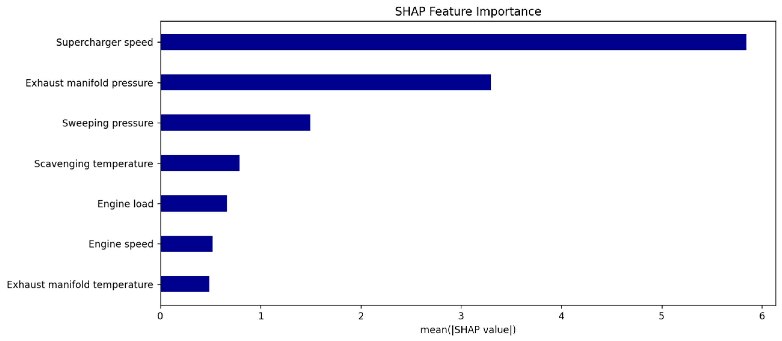
In practical application, we calculated SHAP values based on the trained diffusion model and generated feature importance plots. Figure 8 visually illustrate the varying influence of different features on fuel consumption prediction, with the horizontal axis representing the absolute value of the average contribution to predictions and the vertical axis ranking features by importance from highest to lowest. Unlike traditional methods, SHAP not only identifies which features have the greatest impact on predictions but also reveals whether these features exert a positive or negative influence on individual sample predictions, thus providing a foundation for more granular sample-level explanations. Furthermore, the SHAP analysis results offer data-driven support for system optimization, facilitating the validation of the model’s predictive rationality and scientific validity from a physical mechanism perspective, thereby enhancing the model’s interpretability and engineering applicability.

The SHAP feature importance analysis results, as depicted in the figure, reveal that turbocharger speed (mean|SHAP| ≈ 5.8) is the most significant variable influencing diesel engine fuel consumption predictions, with its average SHAP value substantially exceeding that of other features, indicating its dominant impact on model outputs. Following this, exhaust manifold pressure (mean|SHAP| ≈ 3.3) and scavenging pressure (mean|SHAP| ≈ 1.5) also exhibit notable influences on the model’s predictions.

From the perspective of diesel engine physical mechanisms, higher turbocharger speeds increase intake air volume per unit time, enhancing charge efficiency and promoting more complete combustion, which improves thermal efficiency and may reduce specific fuel consumption. Exhaust manifold pressure and scavenging pressure collectively affect the cylinder’s gas exchange process. Optimizing these parameters can reduce exhaust gas residuals and increase fresh air charge, thereby enhancing combustion efficiency.

Other variables, such as scavenging temperature, engine load, engine speed, and exhaust manifold temperature, have average SHAP values ranging between 0.5 and 1.0, indicating a lower contribution to the model. This suggests that while these factors influence combustion conditions and fuel injection strategies to some extent, their impact is relatively minor.

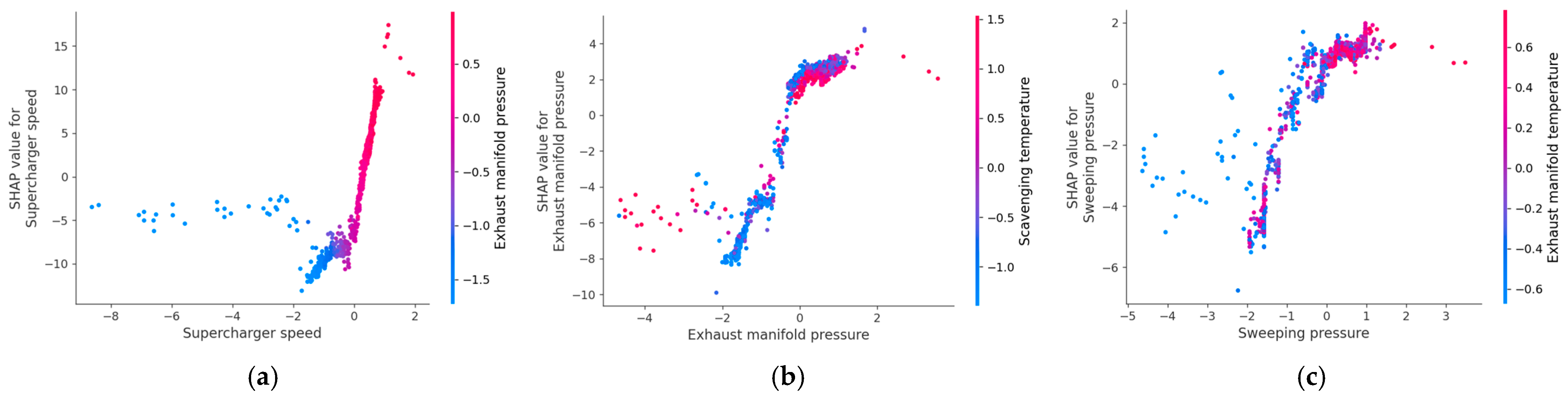
Figure 9 shows the sensitivity analysis of the first three relevant parameters. The SHAP dependence analysis for turbocharger speed shows that as the turbocharger speed increases from lower negative values, the SHAP value rises rapidly from negative to positive, indicating a positive contribution of turbocharger speed to the model’s prediction of unit fuel consumption. This may reflect the mechanism whereby increased engine load at excessively high turbocharger speeds results in elevated fuel consumption. The color transition from blue to red represents the increase in exhaust manifold pressure, and in the mid-to-high turbocharger speed range, higher exhaust manifold pressure corresponds to higher SHAP values, suggesting a clear positive interaction between the two.

For exhaust manifold pressure, the SHAP dependence plot reveals a trend where the SHAP value initially decreases and then increases as exhaust manifold pressure rises, indicating a nonlinear effect on fuel consumption. Notably, when exhaust manifold pressure is in the intermediate range (close to a standardized value of 0), the SHAP value is minimized, suggesting reduced fuel consumption. Beyond this range, fuel consumption increases again. The color represents scavenging temperature, showing a more pronounced positive correlation between exhaust manifold pressure and fuel consumption at higher temperatures.

Sensitivity analysis of scavenging pressure reveals that the SHAP value generally increases monotonically with rising scavenging pressure, meaning higher scavenging pressure leads to greater predicted fuel consumption. The color represents exhaust manifold temperature, with the effect of scavenging pressure being more significant at higher temperatures. Overall, scavenging pressure has a positive impact on fuel consumption without a distinct inflection point.

This local sensitivity analysis based on SHAP dependence plots not only quantitatively reveals the direction and strength of the influence of key variables on fuel consumption predictions but also highlights their nonlinear relationships and interaction effects between variables. These insights provide empirical support for optimizing diesel engine control strategies.

3.3. Data Enhancement and Optimization Framework

The real ship data used in the experiment has problems such as high dimension, inconsistent scale, significant noise interference, and frequent outliers and missing values. Directly using the original data will reduce the prediction accuracy and the effect of the model. To address these issues, a Diesel Engine Data Enhancement and Optimization Framework (DEOF) is developed.

Firstly, missing values are a common issue during data collection, often caused by sensor malfunction, communication errors, or recording mistakes. The proper handling of missing data is crucial to maintaining data continuity and accuracy. Therefore, both forward-filling and backward-filling methods are employed to impute missing values. Let ${\mathrm{x}}_{\mathrm{i}}$ denote a data point; the filling methods can be expressed as follows:

$${\mathrm{x}}_{\mathrm{i}}=\left\{\begin{array}{c}{\mathrm{x}}_{\mathrm{i}-1}, \mathrm{If} \mathrm{you} \mathrm{use} \mathrm{forward} \mathrm{filling}\\ {\mathrm{x}}_{\mathrm{i}+1}, \mathrm{If} \mathrm{you} \mathrm{use} \mathrm{backward} \mathrm{filling}\end{array}\right.$$

(13)

Outliers refer to observations that are significantly different from other data points in the dataset, often caused by measurement errors or extreme events. In this study, the Z-score method is used to detect outliers. The Z-score calculates the degree of deviation of each data point from the mean and is given by the following formula:

$${\mathrm{Z}}_{\mathrm{i}}={\displaystyle \frac{{\mathrm{x}}_{\mathrm{i}}-\mathsf{\mu }}{\mathsf{\sigma }}}$$

(14)

where ${\mathrm{x}}_{\mathrm{i}}$ is the data point, $\mathsf{\mu }$ is the sample mean, and $\mathsf{\sigma }$ is the sample standard deviation. If $\left|{\mathrm{Z}}_{\mathrm{i}}\right|>3$, the data point is considered an outlier and is removed from the dataset.

Similarly, time features are of significant importance for predicting diesel engine fuel consumption, as fuel consumption may be influenced by time periods, seasonal variations, and other cyclical factors. By extracting features such as hour, day, week, and month from the original timestamp, the model can learn time dependencies. For example,

Hour Feature: ${\mathrm{t}}_{\mathrm{h}\mathrm{o}\mathrm{u}\mathrm{r}}=\mathrm{H}\mathrm{o}\mathrm{u}\mathrm{r}\left(\mathrm{t}\right)$;

Day Feature: ${\mathrm{t}}_{\mathrm{d}\mathrm{a}\mathrm{y}}=\mathrm{D}\mathrm{a}\mathrm{y}\left(\mathrm{t}\right)$;

Month Feature: ${\mathrm{t}}_{\mathrm{m}\mathrm{o}\mathrm{n}\mathrm{t}\mathrm{h}}=\mathrm{M}\mathrm{o}\mathrm{n}\mathrm{t}\mathrm{h}\left(\mathrm{t}\right)$;

Week Feature: ${\mathrm{t}}_{\mathrm{w}\mathrm{e}\mathrm{e}\mathrm{k}}=\mathrm{W}\mathrm{e}\mathrm{e}\mathrm{k}\left(\mathrm{t}\right)$.

These features provide the model with information about time patterns, enabling it to identify the relationship between time and fuel consumption.

In many applications, short-term fluctuations can lead to instability in the data, necessitating the use of moving averages to smooth the data. Let the window size be $\mathrm{w}$, and the moving average is calculated as follows:

$${\mathrm{M}\mathrm{A}}_{\mathrm{t}}={\displaystyle \frac{1}{\mathrm{w}}}\sum _{\mathrm{i}=\mathrm{t}-\mathrm{w}+1}^{\mathrm{t}}{\mathrm{x}}_{\mathrm{i}}$$

(15)

where ${\mathrm{M}\mathrm{A}}_{\mathrm{t}}$ is the moving average at time $\mathrm{t}$, $\mathrm{w}$ is the window size, and ${\mathrm{x}}_{\mathrm{i}}$ is the data point at time $\mathrm{i}$.

In real-world data, noise may arise from various factors, such as sensor errors, environmental interference, and other sources. The presence of noise can affect the model’s learning ability, especially when dealing with large datasets. To remove noise, this study uses the Savitzky–Golay filter, a filtering method based on local polynomial fitting. Assuming the data $\mathrm{y}$ is a time series, the filter formula is given by

$${\mathrm{y}}_{\mathrm{s}\mathrm{m}\mathrm{o}\mathrm{o}\mathrm{t}\mathrm{h}}(\mathrm{t})=\sum _{\mathrm{k}=-\mathrm{m}}^{\mathrm{m}}{\mathrm{a}}_{\mathrm{k}}·{\mathrm{y}}_{\mathrm{t}+\mathrm{k}}$$

(16)

where ${\mathrm{a}}_{\mathrm{k}}$ is the weight coefficient, ${\mathrm{y}}_{\mathrm{s}\mathrm{m}\mathrm{o}\mathrm{o}\mathrm{t}\mathrm{h}}(\mathrm{t})$ is the smoothed data, and ${\mathrm{y}}_{\mathrm{t}+\mathrm{k}}$ is the original data point.

Feature scaling aims to adjust all features to the same scale to prevent certain features from having an outsized influence on the model’s training. Common feature scaling methods include standardization and normalization. In this study, the Min-Max normalization method is used to map the data to the [0, 1] range. The normalization formula is

$${\mathrm{x}}_{\mathrm{s}\mathrm{c}\mathrm{a}\mathrm{l}\mathrm{e}\mathrm{d}}={\displaystyle \frac{\mathrm{x}-{\mathrm{x}}_{\mathrm{m}\mathrm{i}\mathrm{n}}}{{\mathrm{x}}_{\mathrm{m}\mathrm{a}\mathrm{x}}-{\mathrm{x}}_{\mathrm{m}\mathrm{i}\mathrm{n}}}}$$

(17)

where $\mathrm{x}$ is the original data, and ${\mathrm{x}}_{\mathrm{m}\mathrm{i}\mathrm{n}}$ and ${\mathrm{x}}_{\mathrm{m}\mathrm{a}\mathrm{x}}$ are the minimum and maximum values of the data, respectively.

When the dimensionality of the data is too high, the model’s training efficiency can be impacted, and there is also a risk of overfitting. Principal component analysis (PCA) [35] is a practical dimensionality reduction technique widely used in engineering fields, such as data preprocessing and feature extraction, with the goal of simplifying complex datasets into a more manageable form. Its core principle involves mapping data onto a new orthogonal coordinate system, retaining the directions of maximum variance to eliminate redundant information.

In ship fuel consumption prediction, PCA is employed to handle multidimensional engine variables, such as main engine speed and scavenging pressure, extracting the key features that most significantly impact fuel consumption. In practice, the data is first standardized to ensure consistent scales across variables. Then, the principal directions (i.e., principal components) are identified through computation, and the original data is projected onto these directions to produce a reduced-dimensionality result. This approach not only reduces computational burden but also enhances model training efficiency.

3.4. Evaluation Metrics

To comprehensively evaluate the performance of the model proposed in this paper for predicting fuel consumption in marine diesel engines, three evaluation metrics are selected: root mean square error (RMSE), mean absolute error (MAE), and coefficient of determination (R²).

$$\mathrm{R}\mathrm{M}\mathrm{S}\mathrm{E}=\sqrt{{\displaystyle \frac{1}{\mathrm{n}}}\sum _{\mathrm{i}=1}^{\mathrm{n}}{\left({\mathrm{y}}_{\mathrm{i}}-{\widehat{\mathrm{y}}}_{\mathrm{i}}\right)}^2}$$

(18)

$$\mathrm{M}\mathrm{A}\mathrm{E}={\displaystyle \frac{1}{\mathrm{n}}}\sum _{\mathrm{i}=1}^{\mathrm{n}}\left|{\mathrm{y}}_{\mathrm{i}}-{\widehat{\mathrm{y}}}_{\mathrm{i}}\right|$$

(19)

$${\mathrm{R}}^2=1-{\displaystyle \frac{{\sum }_{\mathrm{i}=1}^{\mathrm{n}}{\left({\mathrm{y}}_{\mathrm{i}}-{\widehat{\mathrm{y}}}_{\mathrm{i}}\right)}^2}{{\sum }_{\mathrm{i}=1}^{\mathrm{n}}{\left({\mathrm{y}}_{\mathrm{i}}-\overline{\mathrm{y}}\right)}^2}}$$

(20)

Among these, the root mean square error (RMSE) measures the overall deviation between predicted and actual values, being particularly sensitive to larger prediction errors, thus reflecting the model’s ability to control extreme errors.

The mean absolute error (MAE) is used to quantify the average deviation between predicted and actual values. Compared to the RMSE, the MAE is more robust and less susceptible to the influence of extreme values. In this study, the MAE represents the average prediction error per sample in fuel consumption forecasting, providing a realistic reflection of the overall prediction error level.

Additionally, the coefficient of determination (R²) evaluates the model’s ability to capture the trend of data variation, with values in the range of [0, 1]. A value closer to 1 indicates a better ability of the model to explain the variance between samples.

In summary, these three metrics complement each other: the RMSE highlights the model’s capacity to control large errors, the MAE describes the robustness of the overall error level, and the R² reflects the ability to explain trends. Together, they comprehensively assess the prediction accuracy and stability of the MD-RAN model under complex operating conditions.

4. Results and Discussion

The model used in this study is implemented based on the PyTorch 3.10 framework. To ensure training efficiency, a CUDA-supported GPU is utilized. During the training process, the model undergoes 300 iterations, with the Adam optimizer used for parameter updates in each iteration. The learning rate for the inner loop is set to 0.01, and the learning rate for the outer loop is set to 0.001. The ratio of the training set to the validation set is 8:2.

To further elucidate the structural design and forward propagation mechanism of the proposed MD-RAN Model, Algorithm 1 provides a simplified pseudocode. The pseudocode clearly illustrates the collaborative workflow of the core modules during training, including key steps such as feature perturbation, attention mechanism, residual connection, and output prediction. This representation facilitates an intuitive understanding of how the model processes input data and accomplishes the fuel consumption prediction task in engineering applications, thereby providing a reference for subsequent implementation and algorithm reproduction.

Algorithm 1 Meta-learning Diffusion Residual Attention Network(MD-RAN)
Input: ⟨${\mathrm{X}}_{\mathrm{t}\mathrm{r}\mathrm{a}\mathrm{i}\mathrm{n}},{\mathrm{y}}_{\mathrm{t}\mathrm{r}\mathrm{a}\mathrm{i}\mathrm{n}}$⟩, ⟨${\mathrm{X}}_{\mathrm{v}\mathrm{a}\mathrm{l}},{\mathrm{y}}_{\mathrm{v}\mathrm{a}\mathrm{l}}$⟩, num_epochs, num_tasks
Output: ⟨$\mathsf{\theta },\mathrm{u}\mathrm{p}\mathrm{d}\mathrm{a}\mathrm{t}\mathrm{e}\mathrm{d}$⟩
1.	Initialize model parameters
2.	⟨$\mathsf{\theta }$⟩ ← Initialize⟨${\mathrm{f}}_{\mathrm{c}1},{\mathrm{f}}_{\mathrm{c}2},{\mathrm{f}}_{\mathrm{c}3}$⟩, ⟨attention⟩, ⟨dropout⟩, ⟨residual_weight⟩
3.	for epoch = 1 to num_epochs do
4.	Sample tasks for meta-learning
5.	for each task in num_tasks do
6.	⟨${\mathrm{X}}_{\mathrm{t}\mathrm{a}\mathrm{s}\mathrm{k}},{\mathrm{y}}_{\mathrm{t}\mathrm{a}\mathrm{s}\mathrm{k}}$⟩ ← Sample from ⟨${\mathrm{X}}_{\mathrm{t}\mathrm{r}\mathrm{a}\mathrm{i}\mathrm{n}},{\mathrm{y}}_{\mathrm{t}\mathrm{r}\mathrm{a}\mathrm{i}\mathrm{n}}$⟩
7.	Inner_steps ← max(1, int(5 × (1 − epoch/num_epochs)))
8.	Inner loop: Task-specific training
9.	for step = 1 to inner_steps do
10.	⟨${\mathrm{X}}_{\mathrm{t}\mathrm{a}\mathrm{s}\mathrm{k}}^{\prime }$⟩ ← ⟨${\mathrm{X}}_{\mathrm{t}\mathrm{a}\mathrm{s}\mathrm{k}}$⟩ + 0.1 × N(0, 1)
11.	⟨${\widehat{\mathrm{y}}}_{\mathrm{t}\mathrm{a}\mathrm{s}\mathrm{k}}$⟩ ← fc3(⟨ dropout(ReLU(fc2(attention(ReLU(fc1(⟨${\mathrm{X}}_{\mathrm{t}\mathrm{a}\mathrm{s}\mathrm{k}}^{\prime }$⟩))))))⟩ + residual_ weight × ${\mathrm{f}\mathrm{c}}_{\mathrm{r}\mathrm{e}\mathrm{s}\mathrm{i}\mathrm{d}\mathrm{u}\mathrm{a}\mathrm{l}}$(⟨${\mathrm{X}}_{\mathrm{t}\mathrm{a}\mathrm{s}\mathrm{k}}^{\prime }$⟩))
12.	⟨${\mathrm{L}}_{\mathrm{t}\mathrm{a}\mathrm{s}\mathrm{k}}$⟩ ← MSE(⟨${\widehat{\mathrm{y}}}_{\mathrm{t}\mathrm{a}\mathrm{s}\mathrm{k}},{\mathrm{y}}_{\mathrm{t}\mathrm{a}\mathrm{s}\mathrm{k}}$⟩); update⟨${\mathsf{\theta }}^{\prime }$⟩
13.	Outer loop: Meta-learning optimization
14.	⟨${\widehat{\mathrm{y}}}_{\mathrm{v}\mathrm{a}\mathrm{l}}$⟩ ← model(⟨${\mathrm{X}}_{\mathrm{v}\mathrm{a}\mathrm{l}}$⟩, 0.1 × (1 − epoch/num_epochs)); ⟨${\mathrm{L}}_{\mathrm{m}\mathrm{e}\mathrm{t}\mathrm{a}}$⟩←⟨${\mathrm{L}}_{\mathrm{m}\mathrm{e}\mathrm{t}\mathrm{a}}$⟩ + MSE(⟨${\widehat{\mathrm{y}}}_{\mathrm{v}\mathrm{a}\mathrm{l}},{\mathrm{y}}_{\mathrm{v}\mathrm{a}\mathrm{l}}$⟩)
15.	update ⟨$\mathsf{\theta }$⟩ ← ⟨$\mathsf{\theta }$⟩ − outer_lr × ${\nabla }_{\mathsf{\theta }}$⟨${\mathrm{L}}_{\mathrm{m}\mathrm{e}\mathrm{t}\mathrm{a}}$⟩
16.	return ⟨$\mathsf{\theta },\mathrm{u}\mathrm{p}\mathrm{d}\mathrm{a}\mathrm{t}\mathrm{e}\mathrm{d}$⟩

This algorithm implements a meta-learning framework with an enhanced diffusion model for efficient task adaptation. It initializes a model with fully connected layers, multi-head attention, dropout, and a residual connection (steps 1–2). The training loops over epochs and tasks (steps 3–5), dynamically adjusting inner steps (step 7). In the inner loop (steps 9–12), it adds noise for diffusion, processes data through the model layers, and updates task-specific parameters. The outer loop (steps 13–14) performs meta-optimization by accumulating validation loss and updating global parameters. Finally, it returns the optimized parameters (step 16).

4.1. Model Optimization and Comparison

In the MD-RAN architecture proposed in this paper, the diffusion model is applied as the core modeling unit to the host parameter-based regression task. Traditionally, diffusion models are widely applied in image generation, with the fundamental principle of gradually adding noise to data in the forward process, transforming it into a standard Gaussian distribution, and then using a deep neural network to learn the mapping function for recovering the original data from noise in the reverse process. To adapt this mechanism to regression problems, particularly for engine fuel consumption prediction, this study makes targeted adjustments to the input structure, network design, and training strategy.

Unlike image tasks that involve spatially structured 2D pixel matrices, the data processed in this study consists of multiple engine operating parameters and time-derived features, representing the operating state of a diesel engine at a specific time point. After standardization, these features are organized into fixed-dimensional vectors as model inputs, effectively translating the concept of “data points” in diffusion models into “operating state context features”. Subsequently, Gaussian noise of varying intensities is introduced in each training step to simulate interference factors in real-world conditions. This “perturbation–recovery” process effectively enhances the model’s robustness to input disturbances and improves its adaptability to anomalous fluctuations.

To further capture complex interactions between features, MD-RAN incorporates a multi-head attention mechanism and a dynamic residual connection module into the main network structure. The attention mechanism models dependencies between engine parameters, extracting key patterns from the operating state. The dynamic residual connection, by introducing a learnable weight parameter, enables the model to dynamically adjust the fusion ratio between the original input and deep features based on the current task, thereby preserving critical information and enhancing the network’s nonlinear expressive capacity.

For model training, this study adopts the Model-Agnostic Meta-Learning (MAML) algorithm from meta-learning. This approach combines inner and outer loops to enable rapid adaptation to small-sample tasks. In each round of training, the model performs inner-loop fast updates on multiple randomly sampled task subsets and outer-loop parameter optimization on the entire validation set. Notably, to further improve training stability, this study dynamically adjusts the inner-loop steps and introduces validation loss in the outer loop for global guidance, achieving meta-level learning of the optimization path.

Finally, the model output is a continuous value that has been de-standardized, corresponding to the fuel consumption of the main engine at the target time point. This regression output format differs from the image generation goals of traditional diffusion models, highlighting the model’s adaptability to industrial regression tasks. In summary, the MD-RAN architecture integrates the noise modeling capability of diffusion models, the global feature capture ability of the attention mechanism, the structural stability of residual connections, and the rapid adaptability of meta-learning strategies. This combination enables the precise modeling and prediction of the relationship between engine operating parameters and fuel consumption, demonstrating the broad application potential of diffusion models in non-image domains.

To prove the rationale of this study, five groups of comparative experiments are set up, the main purpose of which is to optimize the diffusion model itself in a gap-filling manner. Using the original dataset, we first analyze the shortcomings of this model and gradually implement the optimization strategy.

The comparison results of

Table 4. Comparison of model performance before and after optimization.

Module Name	RMSE	MAE	R2
Diffusion	5.1337	3.1944	0.8587
Meta-Diffusion	3.6867	2.5901	0.9271
Meta-DiffuseDynNoise	3.4560	2.4156	0.9360
Meta-DiffuseDynNoiseAttn	3.2818	2.3185	0.9423
Meta-DiffuseDynNoiseAttnRes	3.0817	2.2341	0.9487
MD-RAN	2.9260	2.0533	0.9541

are based on RMSE, MAE, and R² evaluation metrics indicate that the basic diffusion model exhibits poor prediction performance, with weak alignment between predicted and actual values and a relatively scattered distribution of data points. Meta-learning optimization significantly improves prediction accuracy. Further enhancements, including the introduction of dynamic noise adjustment and a multi-head attention mechanism, continuously improve the model’s prediction performance and robustness, reducing errors and aligning the predicted trends more closely with actual values. The addition of dynamic residual connections effectively enhances training stability. Ultimately, the proposed MD-RAN model outperforms all other models, achieving the lowest RMSE (2.9260) and MAE (2.0533) and the highest R² value (0.9541). Considering the average fuel consumption of marine engines under normal operating conditions is 151.70 kg/h, the root mean square error and mean absolute error account for only 1.93% and 1.35% of the average fuel consumption, respectively. This result demonstrates that the model can predict the fuel consumption of marine diesel engines with high accuracy, with errors controlled within acceptable engineering tolerances, validating its effectiveness and usability as a baseline modeling tool for fuel consumption.

4.2. DEOF Comparative Experiment

The data preprocessing steps of DEOF follow an orderly workflow of “data cleaning → feature construction → denoising → normalization → dimensionality reduction,” with clear dependencies between each step. First, after reading the raw data, missing value imputation and outlier detection are performed, where outliers are identified and removed using a Z-score-based method; this ensures data quality as the initial step. Subsequently, temporal features are extracted, and new features are constructed based on the raw data to enhance feature representation. Next, the Savitzky–Golay filter is applied to denoise certain key sensor data, a step completed before normalization to ensure noise does not affect subsequent scaling. Then, all features used for PCA are normalized using MinMaxScaler to mitigate the impact of differing scales on principal component analysis. Finally, the normalized variables were subjected to PCA dimensionality reduction to extract two principal components (PCA_1 and PCA_2) to reduce feature dimensions, remove redundancy, and highlight the main variation direction. This process ensured the quality of diesel engine data and the efficiency of fuel consumption modeling.

As shown in the

Table 5. Comparison of model effects before and after DEOF.

Module Name	Original Data			DEOF Data
	RMSE	MAE	R2	RMSE	MAE	R2
MLP	5.1345	3.0932	0.8586	4.0627	2.6282	0.9052
Random Forest	5.0123	3.0419	0.8653	4.0378	2.6485	0.9064
SVM	5.2651	2.9809	0.8514	4.1691	2.6389	0.9002
ANN	6.1862	3.9842	0.7935	3.7070	2.1819	0.9017
LSTM	5.4848	3.4784	0.8387	4.1278	2.7051	0.9021
Diffusion	5.1337	3.1944	0.8587	4.0472	2.6371	0.9059
Meta-Diffusion	3.6867	2.5901	0.9271	2.6389	2.0242	0.9600
Meta-DiffuseDynNoise	3.4560	2.4156	0.9360	2.5136	1.8843	0.9637
Meta-DiffuseDynNoiseAttn	3.2818	2.3185	0.9423	2.5300	1.8942	0.9632
Meta-DiffuseDynNoiseAttnRes	3.0817	2.2341	0.9487	2.4217	1.8115	0.9663
MD-RAN	2.9260	2.0533	0.9541	1.5801	1.1879	0.9853

above, all the models used in the paper have been compared before and after DEOF. It can be seen that the feature parameters are cleaned by data, missing values are filled, and outliers are removed; through feature engineering, time features are extracted, moving averages are calculated, and the expressiveness of the model is enhanced; through noise reduction, random fluctuations in the data are reduced; through feature scaling, scale differences between features are eliminated; finally, through PCA dimensionality reduction, data dimensions are reduced and computational efficiency is improved. After these treatments, the prediction effects of all models are improved, proving that this data processing method is very effective for diesel engine data and helps improve the accuracy of the prediction model.

4.3. Ablation Study

The ablation study conducted in this research demonstrates the impact of various module optimizations on the performance of the Diffusion model, with detailed results presented in

Table 6. Ablation study results of the model on the dataset.

Experimental Group	DP	MO	DA	MS	DR	IL	RMSE	MAE	R2
1	√	√	√	√	√	√	1.5801	1.1879	0.9853
2	-	√	√	√	√	√	2.9260	2.0533	0.9541
3	√	√	√	√	√	-	2.4217	1.8115	0.9663
4	-	√	√	√	√	-	3.0817	2.2341	0.9487
5	√	√	√	√	-	-	2.5300	1.8942	0.9632
6	-	√	√	√	-	-	3.2818	2.3185	0.9423
7	√	√	√	-	-	-	2.5136	1.8843	0.9637
8	-	√	√	-	-	-	3.4560	2.4156	0.9360
9	√	√	-	-	-	-	2.6389	2.0242	0.9600
10	-	√	-	-	-	-	3.6867	2.5901	0.9271
11	√	-	-	-	-	-	4.0472	2.6371	0.9059

. In the table, core modules are denoted by abbreviations: DP stands for the Data Processing module, MO for the Meta-Learning Optimization for Efficiency module, DA for the Dynamic Adjustment of Noise Level module, MS for the Multi-Head Self-Attention Mechanism module, DR for the Dynamic Residual Connection module, and IL for the Inner-Loop Optimization module. Different combinations of modules were tested, where a check mark (“√”) indicates the inclusion of the module and a dash (“-”) indicates its exclusion.

On the dataset, the baseline performance of the Diffusion model was RMSE 5.1337, MAE 3.1944, and R² 0.8587. After applying data processing and meta-learning optimization for learning efficiency, the RMSE decreased by 48.6%, the MAE decreased by 36.6%, and the R² increased by 11.8%. The subsequent integration of the multi-head self-attention mechanism, dynamic residual connection, and dynamic noise level adjustment modules further reduced the RMSE by 8.2% and the MAE by 10.5% and improved the R² by 0.7%. Finally, optimizing the inner loop resulted in an additional RMSE reduction of 23.7%, an MAE reduction of 22.2%, and a 1.5% increase in R².

The ablation results highlight the critical role of each module in feature extraction, contextual feature modeling, and fuel consumption prediction. The removal of any individual component leads to a notable degradation in model performance. The effectiveness of the Meta-Diffusion Residual Attention Network (MD-RAN) architecture design and the synergy between modules were further verified.

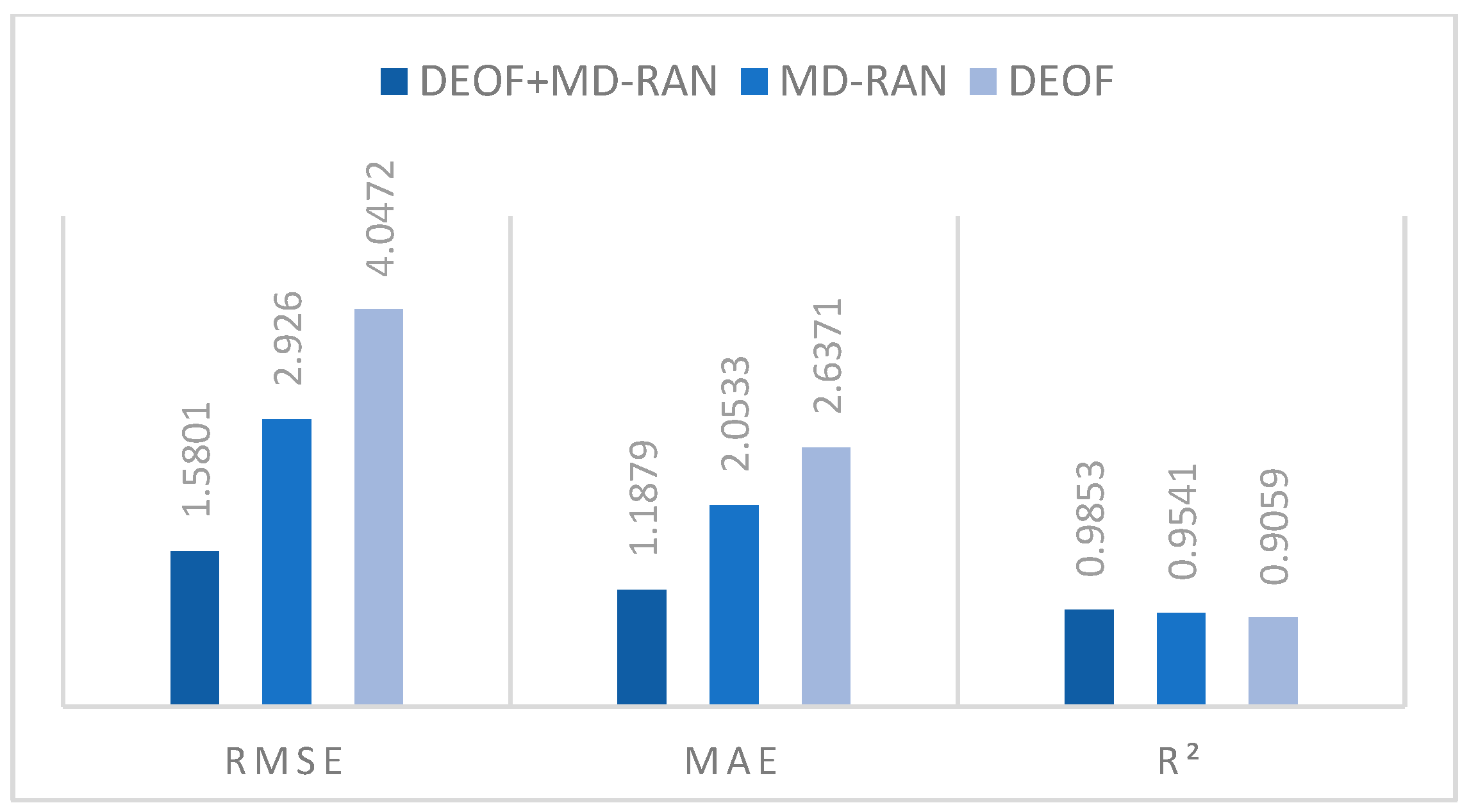
Figure 10 shows two important frameworks of this study are put together for comparative analysis of contribution:

• RMSE: The RMSE of MD-RAN is about 27.7% lower than that of DEOF. DEOF+MD-RAN is further reduced to 1.5801, which is about 46.0% lower than that of MD-RAN;
• MAE: The MAE of MD-RAN is about 22.1% lower than that of DEOF. The MAE of DEOF+MD-RAN is reduced to 1.1879, which is about 42.2% lower than that of MD-RAN;
• R²: The R² of MD-RAN compared to DEOF increased from 0.9059 to 0.9541. DEOF+MD-RAN increased by about 8.8% compared to DEOF and by about 3.3% compared to MD-RAN.

The optimized diffusion model of MD-RAN, when used independently, significantly outperforms DEOF, particularly in reducing the RMSE and MAE, demonstrating a stronger enhancement in prediction accuracy. However, the combined use of DEOF and MD-RAN exhibits a greater synergistic effect, with reductions in the RMSE and MAE far exceeding those achieved by either method alone and the R² reaching its highest value. This indicates that the integration of DEOF’s data processing framework with MD-RAN’s optimized model can more effectively capture data features, further improving the accuracy and explanatory power of fuel consumption prediction.

4.4. Comparison of Model Prediction

After conducting self-optimization experiments, in order to prove the superiority of the experimental algorithm, the effect comparison of different models was analyzed again, and six models, including MLP, Random Forest Regressor, SVM, ANN, LSTM, and Diffusion, were selected for comparison. The parameters of the above models were tuned before the experiment to keep the relevant parameters of the model comparison process consistent. After completing the prediction tasks, performance metrics, including root mean squared error (RMSE) and mean absolute error (MAE), were calculated. The comparative results are summarized in the

Table 7. Comparison of fuel consumption prediction results for different models.

Module Name	RMSE	MAE	R2
MLP	4.0627	2.6282	0.9052
Random Forest	4.0378	2.6485	0.9064
SVM	4.1691	2.6389	0.9002
ANN	3.7070	2.1819	0.9017
LSTM	4.1278	2.7051	0.9021
Diffusion	4.0472	2.6371	0.9059
MD-RAN	1.5801	1.1879	0.9853

below.

From the Table 7 above, it is evident that the MLP model achieves good prediction accuracy, with moderate root mean square error (RMSE) and mean absolute error (MAE) values of 4.0627 and 2.6282, respectively, and an R² value of 0.9052, demonstrating strong nonlinear fitting capability. Random Forest slightly outperforms MLP across these metrics. Although the SVM model performs well in terms of the MAE (2.6389), its RMSE is 4.1691 and R² is 0.9002, indicating a lack of robustness to outliers and high sensitivity to hyperparameter selection. The ANN model shows competitiveness in this task, with an RMSE of 3.7070, an MAE of 2.1819, and an R² of 0.9017. Compared to MLP and Random Forest, ANN achieves noticeable reductions in the RMSE and MAE, reflecting better prediction accuracy, though its R² is slightly lower than that of Random Forest. While the LSTM model is typically well-suited for time series prediction, it does not exhibit significant advantages in this task, with an RMSE of 4.1278, an MAE of 2.7051, and an R² of 0.9021, where lower evaluation metrics suggest poorer adaptability to the task. In contrast, the Diffusion model achieves relatively superior results among baseline models, with an RMSE of 4.0472, an MAE of 2.6371, and an R² of 0.9059, surpassing other comparison methods in overall accuracy and robustness, except for ANN. However, compared to ANN, the Diffusion model’s RMSE and MAE are slightly higher, indicating a slight advantage for ANN in precision.

Following this comparative analysis, the Meta-Diffusion Residual Attention Network (MD-RAN) demonstrates the most outstanding performance. The MD-RAN model achieves an RMSE of 1.5801, an MAE of 1.1879, and a remarkably high R² of 0.9853, significantly surpassing all other models. These results confirm that the model has good fitting accuracy. By incorporating meta-learning optimization, residual connections, and a multi-head attention mechanism, MD-RAN not only enhances its ability to learn complex data representations but also significantly improves its performance on dynamic and complex datasets. The exceptional results indicate that MD-RAN holds strong potential for similar regression tasks, particularly in scenarios involving large-scale, complex data, where it maintains high predictive accuracy and reliability.

4.5. Uncertainty Analysis

To assess the stability and reliability of the results, all experiments were conducted over ten independent repetitions in

Table 8. R² value variations across multiple experimental runs.

Module Name	R2 Mean ± Std
MLP	0.9055 ± 0.0009
Random Forest	0.9068 ± 0.0018
SVM	0.8999 ± 0.0014
ANN	0.9017 ± 0.0019
LSTM	0.9018 ± 0.0011
Diffusion	0.9057 ± 0.0005
MD-RAN	0.9853 ± 0.0001

. From

Table 9. Impact comparison of different training–validation set splits.

Module Name	9:1	8:2	7.5:2.5	7:3	6:4
MLP	0.9053	0.9052	0.8999	0.8917	0.8896
Random Forest	0. 9069	0.9064	0.8996	0.8921	0.8913
SVM	0.9004	0.9002	0.8975	0.8902	0.8827
ANN	0.9032	0.9017	0.8984	0.8894	0.8823
LSTM	0.9102	0.9021	0.8982	0.8909	0.8885
Diffusion	0.9063	0.9059	0.8992	0.8948	0.8906
MD-RAN	0.9856	0.9853	0.9849	0.9840	0.9833

, the model is trained multiple times independently, each time using a different data split: a different training and validation set split, and its performance fluctuations are evaluated.

Different training–validation split ratios can significantly influence the stability and performance of a model. As the proportion of the validation set increases, the model faces greater training difficulty, which may lead to overfitting or underfitting, thereby affecting its performance on the validation set. Especially when the training set is small, the model may still be able to fit the data with fewer samples, but the performance on the test set will be affected. Generally speaking, when the training set ratio is high, the model can learn from more data and perform better. As the training set ratio decreases, the model performance (such as the R²) usually decreases, indicating that the stability of the model is challenged. A more stable model can maintain consistent performance under different data partitions and is not easily affected by data partitions.

It can be seen from the results in Table 9, different models exhibit varying levels of stability under different training–validation split ratios. Both MD-RAN and the Diffusion model demonstrate relatively stable performance across all split settings, with minimal changes in R² values, indicating strong stability. Relatively speaking, the performance of other models fluctuates greatly, especially when the proportion of training sets decreases, and the R² value generally decreases. This indicates that these models may be more susceptible to the impact of data partitioning and show poor stability. Furthermore, when the same model is trained ten times under identical split ratios, the MD-RAN model exhibits extremely low standard deviation, indicating that its performance remains nearly consistent across different runs with minimal fluctuation. This further confirms that MD-RAN possesses exceptional stability and produces highly reliable prediction results.

5. Discussion

First, compared to traditional machine learning-based fuel consumption prediction models and deep learning models, the advantages of MD-RAN lie not only in its integration of diffusion mechanisms and attention mechanisms but also in its meta-learning framework, which enables rapid adaptation to new tasks and operating conditions. This advantage explains the significant improvement in the model’s nonlinear modeling capability under complex scenarios. Additionally, the introduction of dynamic residual connections helps prevent gradient vanishing and enhances training stability. Thus, the results of this study are not merely a natural outcome of algorithmic optimization but also validate the effectiveness of integrating generative models and meta-learning strategies in maritime system modeling, advancing theoretical innovation in prediction and diagnostic methods within this field.

However, these findings must be interpreted within a broader application context. The current model’s training and testing are based on a single type of diesel engine and a relatively limited operational dataset, leaving its generalization ability across different engine types and fuel compositions (e.g., LNG, biodiesel) inadequately validated. Future research should expand the data collection scope to include multiple ship types and diverse operating conditions for cross-domain evaluation, ensuring the model’s transferability and reliability in real-world, varied applications.

Regarding the issue of computational complexity, although MD-RAN excels in prediction accuracy, its complex multi-module architecture (e.g., multi-head attention, diffusion process, and meta-learning optimization) incurs high computational overhead, which may hinder its deployment in real-time monitoring or embedded systems. Future work should explore lighter deep learning architectures to significantly reduce the model’s parameter size and inference time without sacrificing prediction accuracy, thereby improving deployment feasibility.

In this study, the MD-RAN model demonstrates exceptionally high prediction accuracy, with fluctuations across repeated experiments as low as ±0.0001, indicating a high degree of output stability. This phenomenon reflects the effectiveness of the model’s structural design, particularly the advantages of the attention mechanism and residual connections in feature extraction and information retention.

However, this unusually stable output also cautions us to carefully assess the model’s generalization ability. In scenarios with limited data volume and close alignment between training and test set distributions, the model may overfit the training data, resulting in insufficient responsiveness to input variations. Additionally, the currently small noise perturbations in the diffusion modeling process may make the generation process overly smooth. To enhance the model’s robustness in practical applications, future work can focus on the following improvements:

• Incorporate larger-scale data spanning different time periods and operating conditions to increase sample diversity;
• Optimize the noise scheduling strategy in the diffusion process to enhance perturbation effects;
• Employ regularization techniques such as DropBlock or data augmentation to improve the model’s adaptability to unseen data.

Overall, these improvements will help enhance the model’s generalization ability and practicality in complex maritime scenarios.

6. Conclusions

6.1. Contributions of This Study

During the operation of marine engines, the collected measurement data is often influenced by both external environmental changes (e.g., temperature fluctuations, sea condition variations, and load changes) and internal factors (e.g., mechanical wear and fuel quality differences). These disturbances commonly result in issues such as missing values, noise interference, inconsistent scales, and feature redundancy in the data, which in turn affect the accuracy and stability of subsequent modeling and prediction processes.

To address these challenges, this study proposes a Data Enhancement and Optimization Framework (DEOF), systematically integrating key steps such as data cleaning, feature enhancement, dynamic denoising, scale normalization, and principal component analysis, with the aim of comprehensively improving data quality and modeling reliability.

In terms of experimental results, the data preprocessed by DEOF significantly enhances model prediction performance, as evidenced by the following:

• Both traditional machine learning methods and deep learning approaches show varying degrees of improvement in prediction accuracy;
• Compared to unprocessed data, the MD-RAN model based on DEOF performs exceptionally well in the marine engine fuel consumption prediction task.

Building on high-quality data, this study further proposes a Meta-learning-optimized Diffusion-Residual Attention Network (MD-RAN):

• This model integrates the superior nonlinear generative capability of diffusion models, the feature-focusing ability of the multi-head attention mechanism, the training stability provided by dynamic residual connections, and the rapid adaptive optimization capability enabled by the meta-learning framework;
• Compared to traditional prediction methods, MD-RAN demonstrates stronger predictive capability and robustness, with experimental results showing a 14.2% improvement in prediction accuracy, a 64% reduction in RMSE, and a 55.9% reduction in MAE.

In summary, this study not only provides an effective method for marine engine fuel consumption prediction but also establishes a robust data-driven foundation for intelligent ship operation management and fuel optimization decision-making, demonstrating significant engineering application value and broad prospects for practical deployment.

6.2. Application in the Maritime Industry

Marine engine faults are often manifested through abnormal variations in fuel consumption. The MD-RAN model proposed in this study enables accurate monitoring and prediction of the fuel consumption of marine diesel engines under normal operating conditions, thereby establishing a reliable fuel consumption baseline. By comparing the actual fuel consumption with the predicted baseline, the health status of the engine can be effectively assessed. This approach provides critical technical support for the timely and accurate diagnosis of marine engine faults, contributing to enhanced operational reliability and maintenance decision-making.

As the energy structure of ships evolves toward diversification and greening, the deep integration of machine learning methods with various alternative fuel technologies presents vast research potential. On one hand, it enables the development of more generalized and adaptive intelligent fuel consumption modeling frameworks, capable of dynamically identifying and adjusting to different fuel types, combustion modes, and operational patterns. On the other hand, incorporating environmental parameters into multimodal learning is expected to significantly enhance the model’s generalization capability in complex systems.

In summary, this direction not only facilitates the advancement of green shipping but also provides a solid theoretical foundation and technical support for the development of intelligent maritime systems.