Analysis of Abnormal Sea Level Rise in Offshore Waters of Bohai Sea in 2024

Abstract

The primary contribution of this study lies in analyzing the dynamic drivers during two anomalous sea level rise events in the Bohai Sea through coupled numeric modeling using the Weather Research and Forecasting (WRF) model and the Finite-Volume Community Ocean Model (FVCOM) integrated with the Simulating Waves Nearshore (SWAN) module (hereafter referred to as FVCOM-SWAVE). WRF-derived wind speeds (0.05° grid resolution) were validated against Haiyang-2 (HY-2) scatterometer observations, yielding a root mean square error (RMSE) of 1.88 m/s and a correlation coefficient (Cor) of 0.85. Similarly, comparisons of significant wave height (SWH) simulated by FVCOM-SWAVE (0.05° triangular mesh) with HY-2 altimeter data showed an RMSE of 0.67 m and a Cor of 0.84. Four FVCOM sensitivity experiments were conducted to assess drivers of sea level rise, validated against tide gauge observations. The results identified tides as the primary driver of sea level rise, with wind stress and elevation forcing (e.g., storm surge) amplifying variability, while currents exhibited negligible influence. During the two events, i.e., 20–21 October and 25–26 August 2024, elevation forcing contributed to localized sea level rises of 0.6 m in the northern and southern Bohai Sea and 1.1 m in the southern Bohai Sea. A 1 m surge in the northern region correlated with intense Yellow Sea winds (20 m/s) and waves (5 m SWH), which drove water masses into the Bohai Sea. Stokes transport (wave-driven circulation) significantly amplified water levels during the 21 October and 26 August peak, underscoring critical wave–tide interactions. This study highlights the necessity of incorporating tides, wind, elevation forcing, and wave effects into coastal hydrodynamic models to improve predictions of extreme sea level rise events. In contrast, the role of imposed boundary current can be marginalized in such scenarios.

1. Introduction

Since the early 20th century, global sea level has exhibited a gradual rise under the influence of climate change [1,2,3]. This accelerated rise poses a significant threat to coastal regions, amplifying risks of storm surge [4], flooding [5], and large-scale socio-economic damage [6]. Sea level monitoring primarily relies on two approaches: remote sensing and in situ observations. Satellite-based technologies, such as radar altimeters [7] and GPS-derived measurements [8], enable rapid, large-scale assessments of sea surface height. Meanwhile, traditional methods—including shipborne surveys, moored buoys, and tide gauge stations—remain critical for providing high-resolution, localized data. Advances in oceanographic modeling and computational power have further enhanced our capacity to study sea level dynamics. Numerical models are now widely employed for hindcasting historical trends and predicting future scenarios, with sensitivity experiments proving particularly effective for isolating drivers of extreme sea states [9,10].

During the Seasat mission in 1978 [11], the capabilities of various sensors—including a microwave scatterometer [12], radar altimeter [13], infrared radiometer [14], and synthetic aperture radar (SAR) [15]—were tested. Today, satellites such as MetOp, ERS, Haiyang-2 (HY-2), and Sentinel carry these sensors, providing continuous global ocean observations for atmospheric and oceanographic research. Scatterometers and microwave radiometers [16] are primarily used for sea surface wind monitoring and operate at radar incidence angles greater than 20°. In contrast, radar altimeters have a near-nadir beam angle (<2°) [17], directly measuring sea surface height from reflected signals. Additionally, significant wave height (SWH) and sea level anomaly (SLA) are derived from altimeter data [18]. These remotely sensed products are widely applied in mesoscale and large-scale oceanography, including studies of oceanic eddies [19,20], tropical cyclones [21], and long-term climate analysis [22]. However, the spatial resolution of these products remains relatively coarse—typically 12.5 km for scatterometers, 10 km along altimeter footprints, and 18 km for the Surface Wave Investigation and Monitoring (SWIM) instrument aboard the Chinese–French Oceanography SATellite (CFOSAT) [23]. As a result, they are insufficient for coastal water monitoring. While SAR (e.g., Gaofen-3 (GF-3) [24,25] and Sentinel-1 (S-1) [26]) offers finer resolution and wide swath coverage, its long-term data acquisition over specific regions remains challenging.

Numerical models are powerful tools for hindcasting and predicting atmospheric and oceanic dynamics by solving theoretical equations. Several well-known numerical models are used for atmospheric simulations, including the Weather Research and Forecasting (WRF) model [27], the PSU/NCAR MM5 model [28], the Rapid Refresh (RAP) model [29], and the Global and Regional Assimilation and Prediction System (GRAPES) [30]. Leveraging these models, agencies such as the European Centre for Medium-Range Weather Forecasts (ECMWF) and the National Centers for Environmental Prediction (NCEP) Global Forecast System (GFS) operationally produce global atmospheric reanalysis data [31]. For ocean wave modeling, the predominant numerical models are WAVEWATCH-III (WW3) [32] and Simulating Waves Nearshore (SWAN) [33]. In ocean circulation simulations, commonly used models include the Hybrid Coordinate Ocean Model (HYCOM) [34], the Finite-Volume Community Ocean Model (FVCOM) [35], and the Regional Ocean Modeling System (ROMS) [36]. Notably, FVCOM and SWAN utilize unstructured triangular meshes, which provide better conformity to coastlines. Despite their advantages, numerical forecasting models encounter several technical challenges, such as limited spatial and temporal resolution, uncertainties in initial conditions, and computational constraints—particularly under extreme weather conditions [37].

Numerical models serve as indispensable tools for analyzing ocean dynamics, providing critical insights into underlying mechanisms. Through parameter adjustments and boundary condition modifications, these models enable the simulation of various ocean dynamic processes and their environmental impacts. In this study, the WRF model is employed to hindcast wind fields, which serve as forcing fields for FVCOM and FVCOM-SWAVE. We specifically analyze two seawater backflow events in the offshore waters of the Bohai Sea caused by abnormal sea level rise, i.e., 20–21 October and 25–26 August 2024. The paper is organized as follows: Section 2 describes the datasets, including forcing fields and open boundary conditions for the coupled numerical models, along with validation sources. This section also details the model configurations. Section 3 and Section 4 present the results and discussion, respectively. Section 5 provides concluding remarks.

2. Materials and Methods

In this section, we briefly describe the basic principles of the numerical models WRF and FVCOM-SWAVE. We then present the forcing fields and boundary conditions used in the coupled numerical model (FVCOM-SWAVE). Additionally, we outline the sources for validating the hindcasting results, including HY-2 operational products and tide gauge station data. Finally, we introduce the setup of sensitivity experiments in FVCOM-SWAVE.

2.1. Setups of the WRF

The WRF model, a collaborative atmospheric modeling framework jointly developed by the National Center for Atmospheric Research (NCAR) and the National Oceanic and Atmospheric Administration (NOAA), integrates NCAR climate science expertise with NOAA operational forecasting infrastructure. In this study, WRF version 4.2 was configured to simulate wind fields at a horizontal spatial resolution of 5 km with 34 vertical layers. Simulations were conducted for two distinct periods: (1) 1 August 2024 (00:00 UTC) to 31 August 2024 (00:00 UTC) (30 days) and (2) 1 October 2024 (00:00 UTC) to 30 November 2024 (00:00 UTC) (61 days). Key physical parameterizations included the WSM6 microphysics scheme, the RRTMG radiation scheme [38], the Yonsei PBL scheme [39], the MM5 Monin–Obukhov surface layer scheme [40], and the Noah LSM for land–atmosphere interactions [41]. Initial and lateral boundary conditions for the WRF simulations were derived from the NCEP GFS analysis dataset, which provides data at a 0.25° spatial resolution and 3-hourly temporal intervals. These inputs included vertical profiles of wind speed, air temperature, humidity, and pressure, as well as land surface variables such as terrain height and land-use classification.

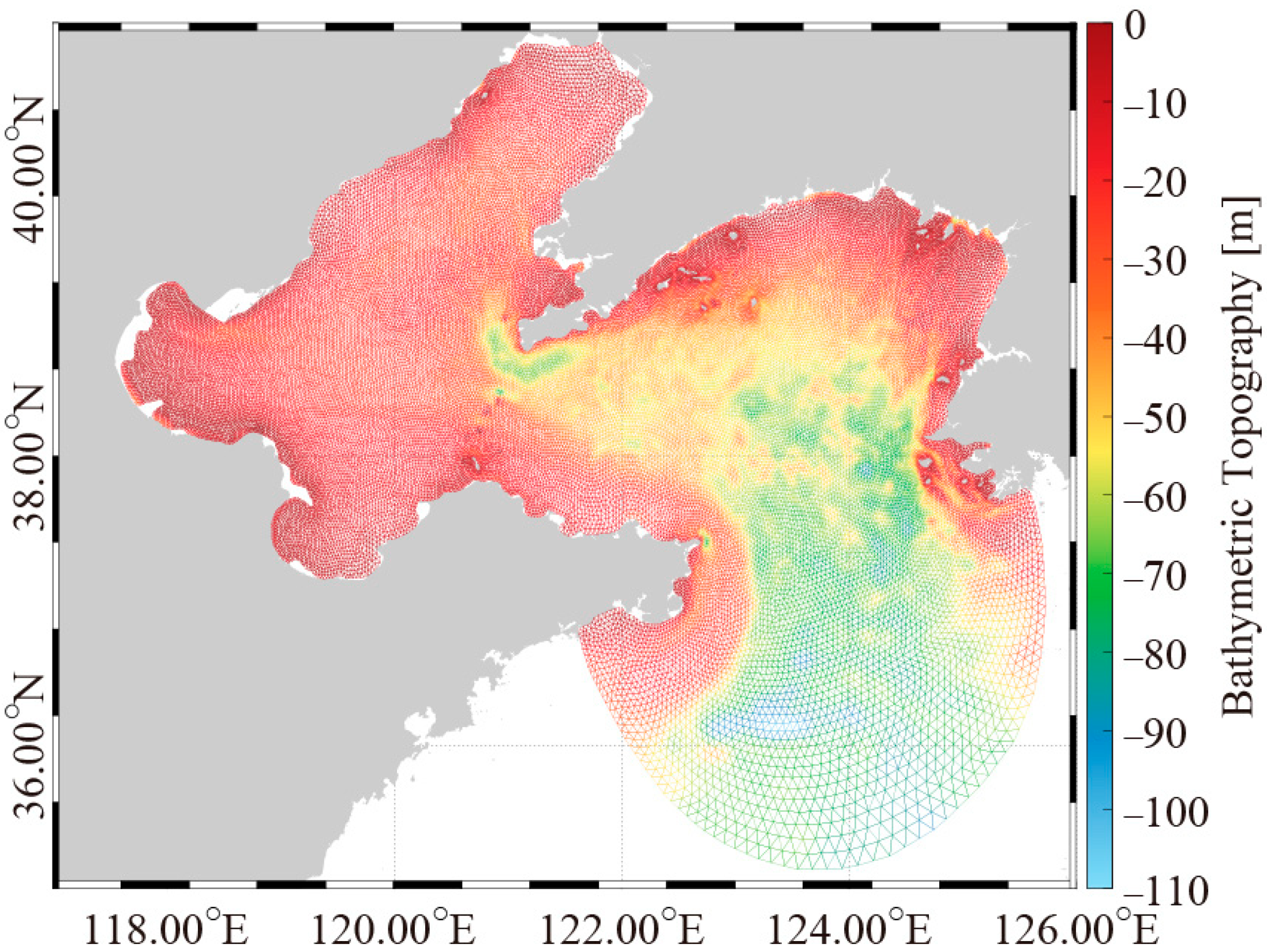
2.2. Setups of FVCOM-SWAVE

FVCOM utilizes an unstructured triangular grid system [42] that provides enhanced geometric flexibility for resolving complex coastal geometries and shallow-water bathymetry. The model’s finite-volume computational framework ensures the accurate representation of hydrodynamic processes across highly irregular topographies while supporting both Cartesian and spherical coordinate systems. For horizontal discretization, FVCOM employs triangular grid elements integrated with the Mellor-Yamada 2.5 (MY-2.5) turbulence closure scheme [43] for subgrid-scale parametrization. Vertical resolution is achieved through generalized terrain-following coordinates (e.g., sigma layers) in conjunction with the Smagorinsky turbulent mixing scheme. FVCOM incorporates a dynamic wet–dry grid cell treatment that accurately simulates tidal flat inundation dynamics. The model solves the fully coupled three-dimensional primitive equations, including momentum balance, mass continuity, and thermodynamic conservation for temperature, salinity, and density fields. This comprehensive approach enables the robust simulation of coastal and oceanographic processes across multiple spatiotemporal scales.

The FVCOM-SWAVE model is a spectral wave modeling system developed by integrating the widely used SWAN framework [44] with the unstructured-grid, finite-volume computational architecture of FVCOM. This synthesis enables fully coupled simulations of hydrodynamic and spectral wave processes in complex coastal and oceanic domains. By retaining the robust spectral wave-solving algorithms of SWAN while incorporating the adaptive spatial discretization of FVCOM, the model achieves enhanced accuracy in resolving irregular geometries, bathymetric gradients, and dynamic wave–current interactions critical for applications such as storm surge propagation and nearshore wave dynamics. The governing equations, adapted from the spectral formulation of SWAN, resolve wave energy evolution, nonlinear wave–wave interactions, and bidirectional wave–current feedback within a three-dimensional hydrodynamic framework. Central to the FVCOM-SWAVE system is the wave action density conservation equation:

$${\displaystyle \frac{\partial N}{\partial t}}+\nabla ·\left[\left(\overrightarrow{C_g}+\overrightarrow{V}\right)N\right]+{\displaystyle \frac{\partial C_{\sigma }N}{\partial \sigma }}+{\displaystyle \frac{\partial C_{\theta }N}{\partial \theta }}={\displaystyle \frac{S_{\mathit{tot}}}{\sigma }}$$

(1)

where N denotes the wave energy density spectrum; t represents the computational time; C_g is the wave group velocity; V is the ambient water velocity; σ denotes the relative wave frequency; θ is the wave direction; C_σ and C_θ represent the wave speed in relative frequency and wave direction, respectively; and S_tot represents the source–sink terms in SWAN. The FVCOM-SWAVE model differentiates itself from SWAN through its numerical schemes. Specifically, it employs the Flux-Corrected Transport (FCT) algorithm in frequency space to minimize numerical diffusion, adopts the implicit Crank–Nicolson method in directional space to enhance stability, and provides explicit and implicit second-order upwind finite-volume schemes in geographic space to handle advection on unstructured grids. In this study, the coupled FVCOM-SWAVE model operates with a temporal resolution of 1 h outputs and an unstructured triangular grid at 0.05° (~5 km) resolution (Figure 1). Leveraging its capability to adapt to complex coastal geometries, the model effectively captures small-scale nearshore phenomena, including waves and currents, while maintaining high computational accuracy in wave dynamics simulations. The simulation period aligns with that of the WRF model, as previously described.

2.3. Forcing Fields and Boundary Conditions in FVCOM-SWAVE

Wind forcing plays a critical role in hindcasting ocean dynamics. However, the spatial resolution of global meteorological datasets such as ECMWF and GFS (0.25° grid) is inadequate for resolving fine-scale processes in coastal waters. The WRF model, designed for meteorological applications across spatial scales ranging from tens of meters to thousands of kilometers, can generate simulations driven by either observational/analysis data or idealized atmospheric conditions. In this study, WRF was configured to simulate wind fields at an enhanced horizontal resolution of 0.05°. To ensure consistency in forcing field data and avoid interpolation errors, the spatial resolution (5 km) of the WRF model was matched to that of FVCOM-SWAVE. These outputs were coupled with the FVCOM-SWAVE system, which employs an unstructured grid architecture to simulate sea surface dynamics. As demonstrated in previous studies [45], wave simulations are sensitive to sea level variability and current interactions. Consequently, the FVCOM-SWAVE simulations were forced using WRF-derived wind fields, along with CMEMS datasets providing sea surface current velocity, salinity, temperature, and sea level at 0.08° spatial resolution and 3-hourly temporal intervals. These inputs were applied as boundary conditions and dynamic forcing fields. Figure 2 illustrates the spatially distributed CMEMS-derived sea surface current speed, sea level, salinity, and temperature fields at 12:00 UTC on 20 October 2024.

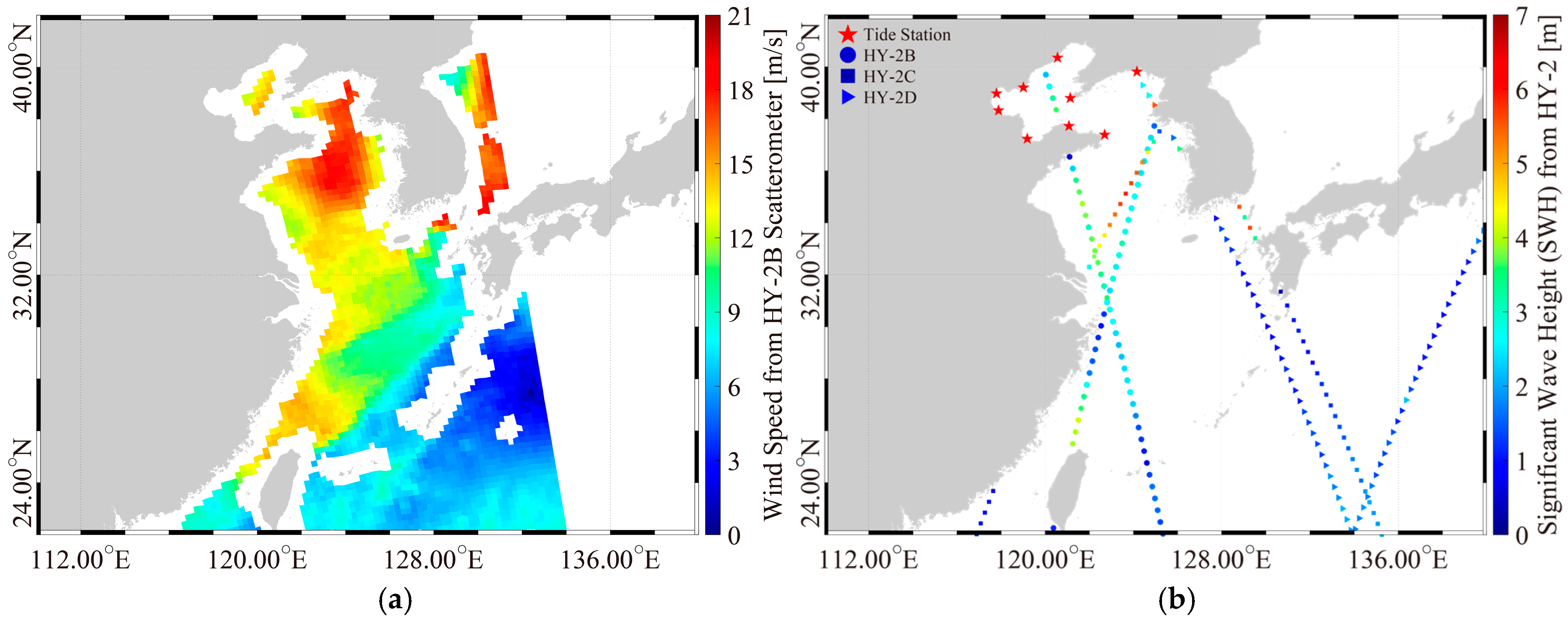
2.4. Validation Sources

The HY-2B satellite, China’s first civilian mission equipped with a scatterometer and altimeter, was launched in 2018. In our prior study [7], the performance of HY-2B data products—categorized into four processing levels: Operational Geophysical Data Records (OGDRs), Interim Geophysical Data Records (IGDRs), Sensor Geophysical Data Records (SGDRs), and Geophysical Data Records (GDRs)—was systematically evaluated. Results demonstrated that the GDR products exhibited superior accuracy. Since 2021, HY-2B’s successor satellites, HY-2C and HY-2D, have been successively launched and operationalized, forming a constellation to enhance oceanographic monitoring. To validate hindcasted wind and wave parameters, non-interpolated operational scatterometer and altimeter data from the HY-2(2B/2C/2D) satellites were obtained from the National Satellite Ocean Application Center (accessible via https://osdds.nsoas.org.cn, accessed on 3 June 2025). HY-2 altimeter and scatterometer products achieve high precision through rigorous processing, including precise orbit determination, instrument calibration, geophysical model integration, and ground validation. Additionally, hourly sea level observations from tide gauge stations along the Chinese coast, provided by the National Marine Information Center and subjected to quality control and analytical processing, were utilized to validate hindcasted sea levels. Figure 3a depicts the HY-2B scatterometer-derived wind speed field at 09:00 UTC on 19 October 2024, while Figure 3b illustrates the concurrent SWH distribution from the HY-2 altimeter. Red five-pointed stars denote the geographical locations of the tide gauge stations used in this study.

2.5. Stokes Transport Calculation

The Stokes drift speed, u_st(z), describes how waves push water particles at different depths. Using a 1D wave spectrum model, it can be expressed as [46]:

$$u_{\mathit{st}}\left(z\right)={\displaystyle \frac{2}{g}}{{\displaystyle \int }}_0^{\infty }{\omega }^3{S}_{\omega }\left(\omega \right){\mathrm{e}}^{2\mathit{kz}}\mathrm{d}\omega$$

(2)

where g denotes gravitational acceleration, ω represents angular frequency, k is the wavenumber, z is the vertical depth coordinate, and S_ω is the 1D wave spectrum. Earlier work [31] simplified this using SWH (H_s) and mean wave period (T_m), through the linear dispersion relation:

$$\stackrel{\rightharpoonup }{u_{\mathit{st}}}\left(z\right)=\stackrel{\rightharpoonup }{u_0}{\mathrm{e}}^{{\displaystyle \frac{{8\pi }^{2}z}{{\mathit{gT}}_m^2}}}$$

(3)

The Stokes drift induces a net Lagrangian transport, commonly referred to as Stokes transport. Integrating Stokes drift velocity over depth gives the Stokes transport vector (Tₛ) and water depth D in the vertical direction:

$$T_s=\mathsf{\pi }{\displaystyle \frac{H_s^2}{T_m}}·\stackrel{\rightharpoonup }{D}$$

(4)

2.6. Statistic Parameter Formula

The model–observation agreement was quantified using three statistical metrics:

$$\mathrm{RMSE}=\sqrt{{\displaystyle \frac{1}{N}}{\displaystyle \sum }_{i=1}^N{\left(p_i-q_i\right)}^2}$$

(5)

$$\mathrm{Cor}={\displaystyle \frac{{\sum }_{\mathrm{i}=1}^N\left(p_i-\overline{p}\right)\left(q_i-\overline{q}\right)}{\sqrt{{\sum }_{i=1}^N{\left(p_i-\overline{p}\right)}^2{\sum }_{i=1}^N{\left(q_i-\overline{q}\right)}^2}}}$$

(6)

$$\mathrm{Bias}={\displaystyle \frac{1}{N}}{\displaystyle \sum }_{i=1}^N\left(p_i-q_i\right)$$

(7)

where p_i denotes the observed values (e.g., satellite measurements), q_i represents the simulated values (e.g., model outputs), N is the total number of collocated data points, and $\overline{p}$ and $\overline{q}$ are the arithmetic means of the observed and simulated values, respectively.

3. Results

This section presents validation results for the hindcasted variables. Subsequently, a sensitivity experiment is conducted to examine sea level variations during seawater backflow events. Finally, the relationships between wind speed, SWH, current velocity, and sea level are analyzed.

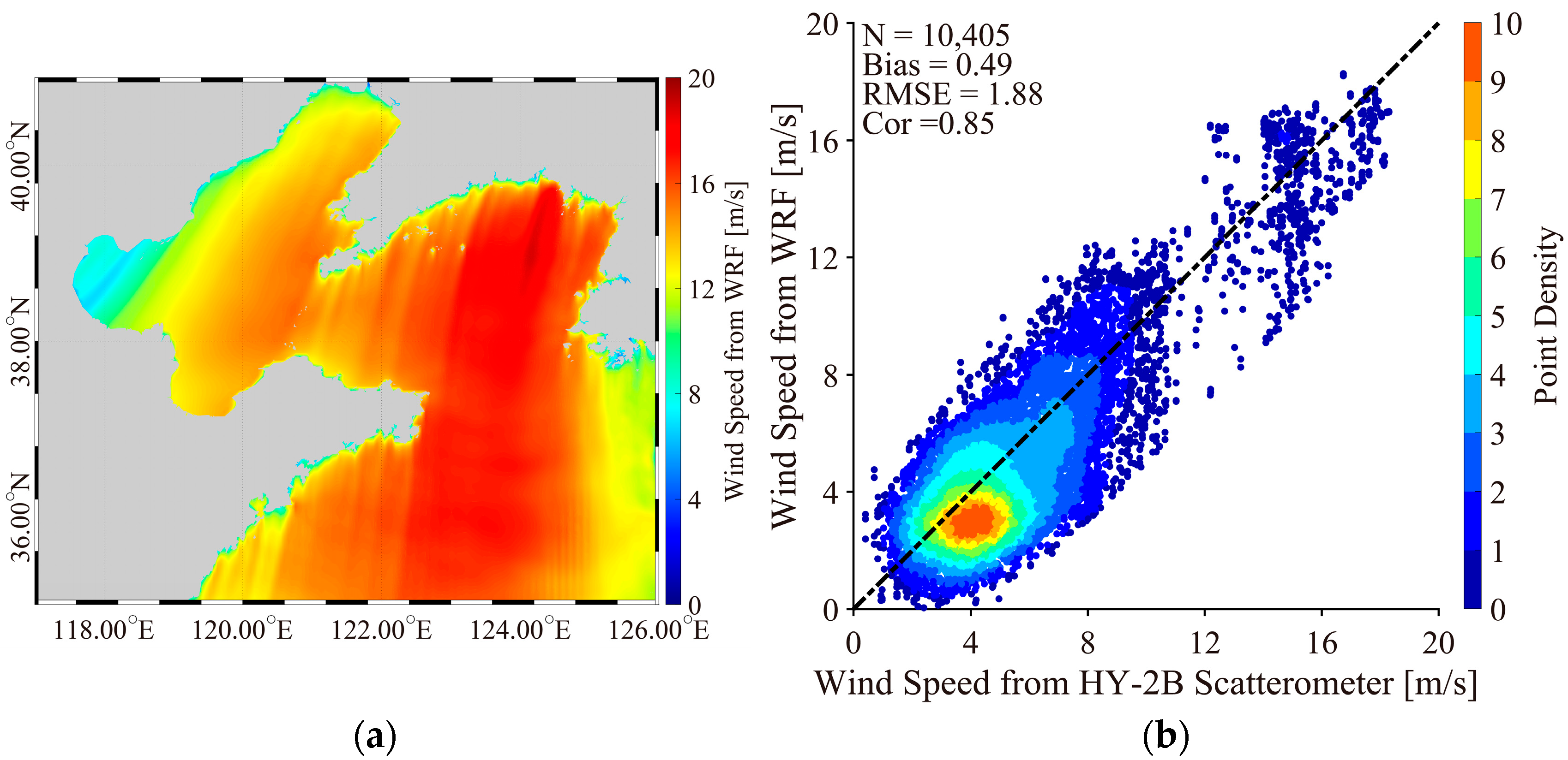
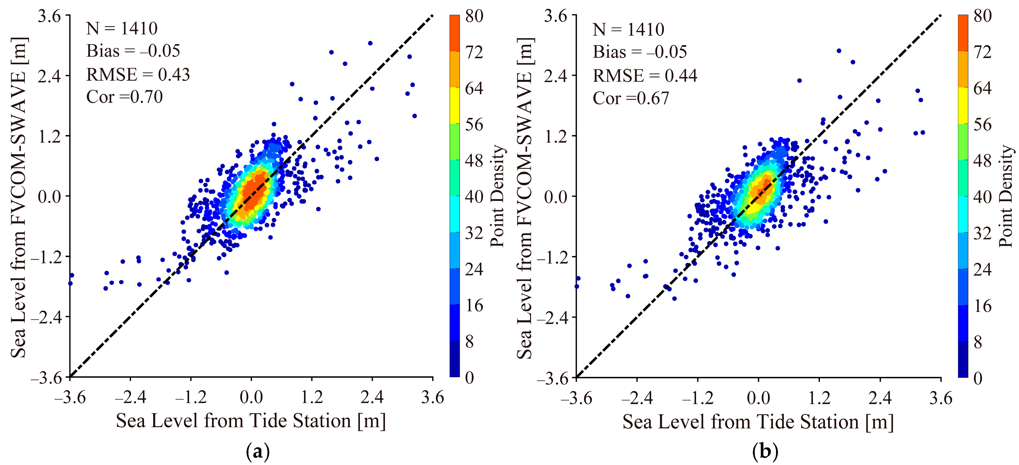
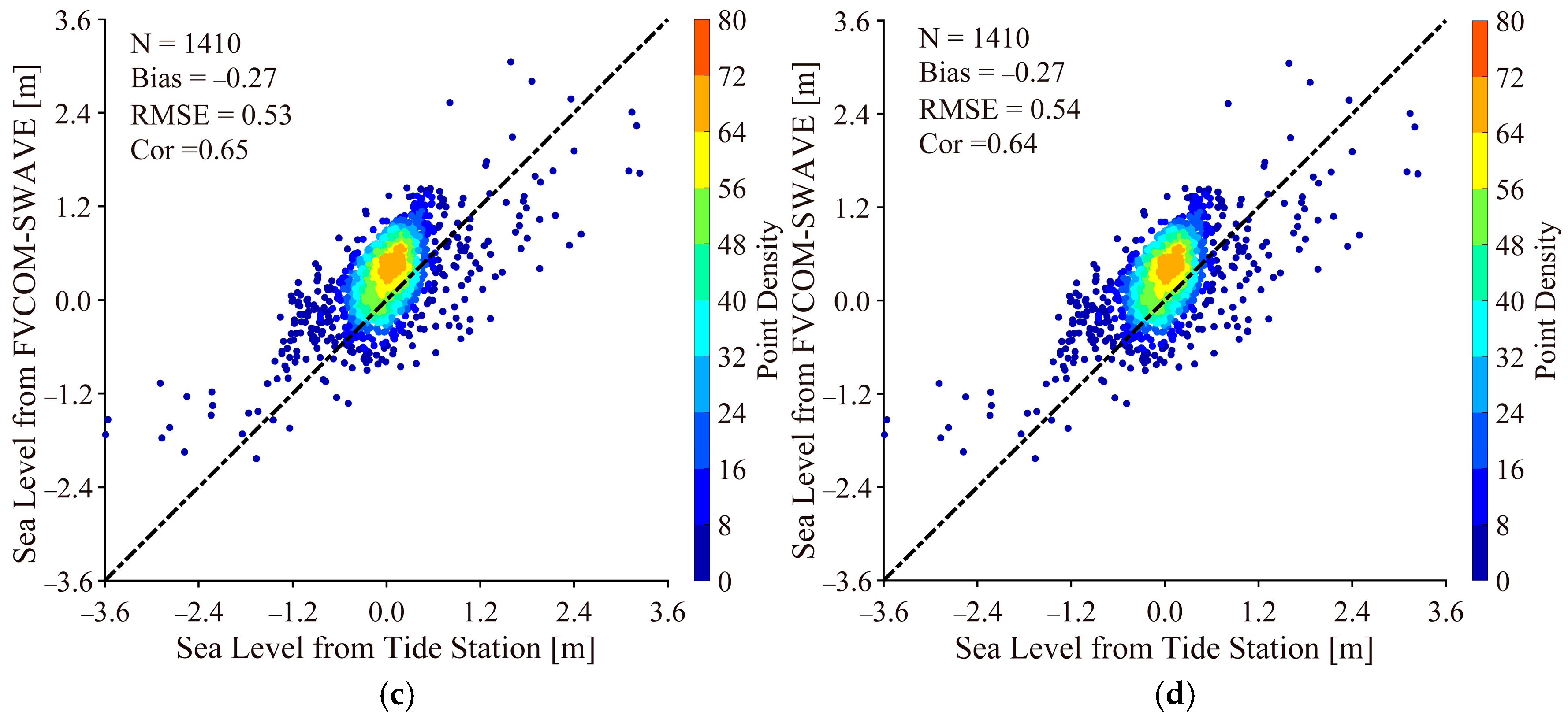
3.1. Validation

Figure 4a presents the WRF-simulated wind field on 19 October 2024 at 09:00 UTC, while Figure 4b displays the corresponding validation using HY-2B/2C/2D scatterometer wind speed measurements. Over 10,000 collocated data points were obtained within the study domain. The temporal mismatch between model outputs and satellite observations was maintained below 10 min to ensure comparability. Quantitative analysis reveals excellent model performance, with a root mean square error (RMSE) of 1.88 m/s and a correlation coefficient (Cor) of 0.85. These results demonstrate strong agreement between WRF simulations and HY-2 scatterometer wind speed observations. Similarly, Figure 5a shows that FVCOM-SWAVE simulated the SWH field on 26 October 2024 at 00:00 UTC, with colored triangles indicating concurrent HY-2 altimeter measurements. The validation yields an RMSE of 0.67 m and Cor of 0.84, indicating good consistency between model results and satellite observations (model outputs and satellite observations were maintained below 30 min). This confirms the model’s capability to accurately reproduce wave conditions as observed by the HY-2 altimeter.

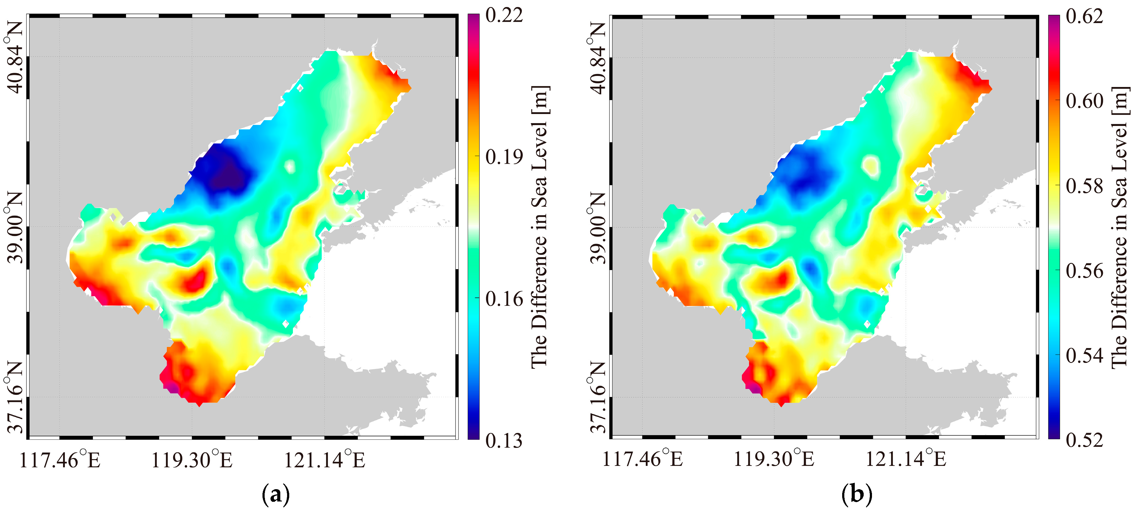
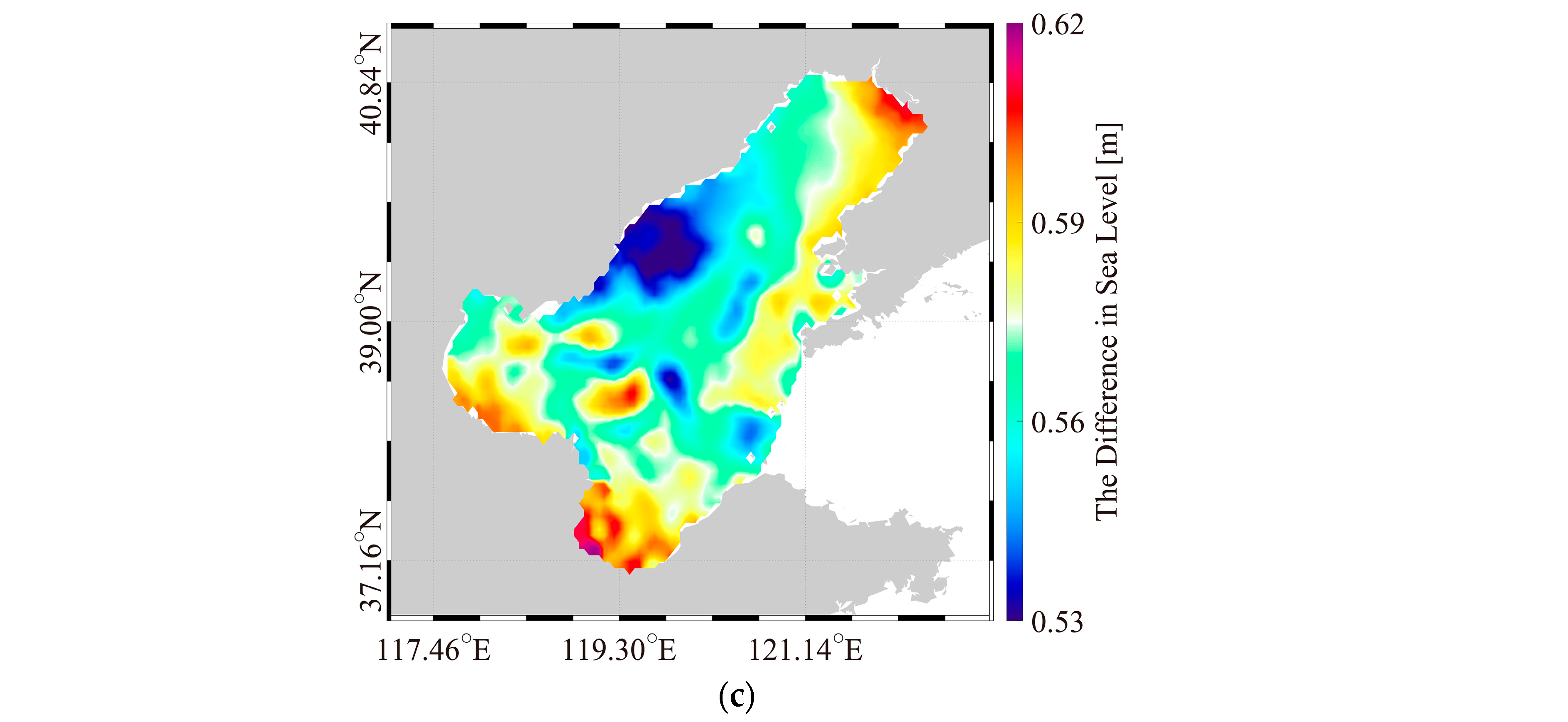
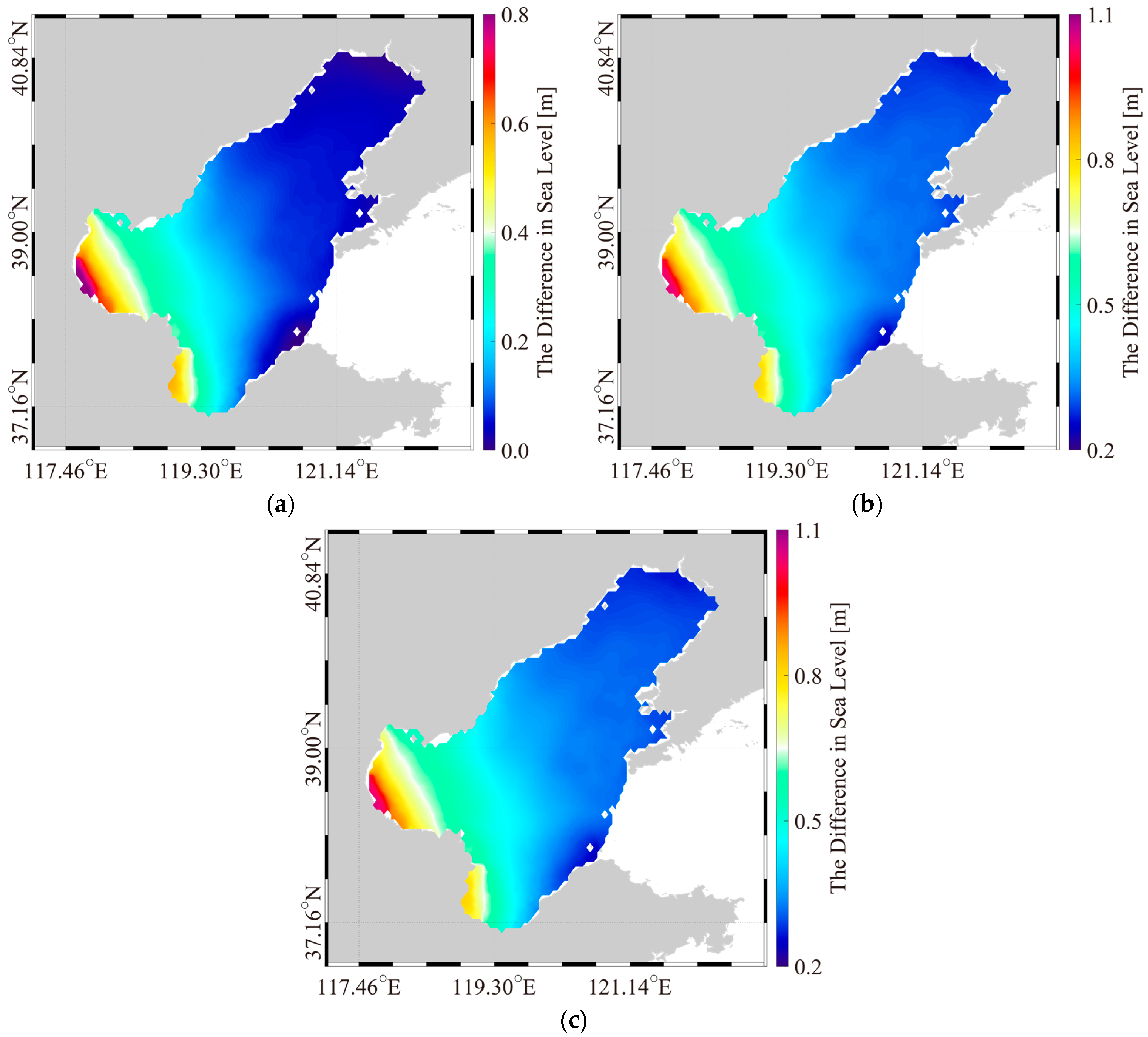
3.2. Sensitive Experiment

To examine the influence of different forcing conditions on model performance, we conducted four sensitivity experiments. All four forcing modes utilize temperature and salinity data from CMEMS as the initial conditions, with distinct configurations applied incrementally: Mode A employs tide forcing exclusively; Mode B integrates both wind and tide forcing; Mode C enhances this framework by combining wind and tide forcing while prescribing water level constraints at the open boundary; finally, Mode D extends the complexity of Mode C by incorporating additional velocity boundary conditions alongside water level specifications at the open boundary.

Figure 6 presents the time series validation between FVCOM-SWAVE-simulated sea levels and tide gauge observations. The results demonstrate that simulations incorporating wind, tide, and elevation forcing fields effectively reproduce observed high sea level conditions. Conversely, simulations with tidal forcing alone accurately capture low sea level variations, particularly at the tide station located at (117.79° E, 38.97° N) (Figure 6a). The comparison of different forcing configurations reveals that elevation and wind are key drivers of water level variability in the study area, while tidal forcing represents the fundamental mechanism governing sea level changes. Notably, currents appear to have negligible influence on sea level variations. Quantitative validation against tide gauge data (Figure 7) shows optimal model performance when considering only tidal effects, yielding an RMSE of 0.43 m and a Cor of 0.70. All four sensitivity experiments maintained RMSE values below 0.70 m, demonstrating consistent model performance across different forcing configurations. These results confirm the reliability of the model for future applications in the study region.

To investigate the influence of seawater backflow events in the offshore waters of the Bohai Sea, sea level simulations from FVCOM-SWAVE on 20 October 2024 and 26 August 2024 were analyzed under distinct forcing configurations. Figure 8 illustrates the spatial differences in sea level between three experimental cases and the baseline tide-only simulation on 20 October 2024: (a) wind and tide, (b) wind, tide, and elevation, and (c) wind, tide, elevation, and current. The results demonstrate a pronounced sea level rise in the northern and southern regions of the Bohai Sea. Notably, the imposed forcing field (elevation and current) exerted a significantly stronger influence than wind forcing, inducing sea level deviations of up to 0.6 m. Similarly, the sea level simulations from FVCOM-SWAVE on 26 August 2024 are presented in Figure 9. The comparison result in Figure 9 shows the similar trend of sea level difference in Figure 8, with sea level deviations of up to 1.1 m. In contrast, the inclusion of the current forcing field exhibited negligible impact on sea level variability, consistent with the statistical findings presented earlier.

3.3. The Relationship Between the Wind Speed, SWH, Imposed Boundary Current, and Sea Level

To investigate the influence of sea surface parameters—wind speed, SWH, and current (mainly imposed boundary current) velocity—on sea level dynamics, we analyzed differences in simulated sea level (calculated by subtracting 20 October results from 21 October outputs), alongside concurrent wind speed simulated by WRF, SWH, and imposed boundary current velocity simulated by FVCOM-SWAVE fields for 20 October 2024. The sea level anomaly map (Figure 10a) reveals a pronounced rise of up to 1 m in the northern Bohai Sea, consistent with observed seawater backflow events in offshore regions. This anomaly correlates with elevated wind speeds (>20 m/s) and SWH (>5 m) in the adjacent Yellow Sea (Figure 10b,c), suggesting that wind- and wave-driven Stokes transport may have displaced water masses toward the Bohai Sea. In contrast, imposed boundary current velocities exhibited no significant correlation with sea level fluctuations (Figure 10d), underscoring the limited role of advective processes in this event. Time series analysis (Figure 11) further demonstrates that the pre-event period (20 October) was characterized by extreme wind and wave conditions, which subsided prior to the peak sea level rise on 21 October. Additionally, Figure 12 shows the time series analysis of the FVCOM-SWAVE simulation during the August 2024 results. The wind speed, imposed boundary current, sea level, and SWH in the Bohai area exhibit climatological periodic variations [47,48], and there is a certain correlation between sea level height and wind speed, SWH, and imposed boundary current. During periods of sea level rise (18–22 October and 26–27 August), these parameters simultaneously peak, and the consistent direction of wind speed and flow velocity drives water masses toward the Bohai Sea. These findings suggest that the combined effects of wind, waves, and currents contribute to anomalous sea level rise. This highlights a complex ocean–atmosphere interaction, where wind speed variations influence wave generation and sea level changes, subsequently altering current velocity and direction.

4. Discussion

Stokes transport along the transect marked in Figure 11a (black line) was computed using wave parameters simulated by the FVCOM-SWAVE model. Figure 13a provides a schematic representation of cross-regional transport dynamics between the Bohai and Yellow Seas, where net inflow into the Bohai Sea is defined as positive. Figure 13b compares the time series of net transport under three distinct forcing configurations during October 2024: (1) tide-only, (2) combined wind, tide, current, and elevation boundary conditions, and (3) wave-induced Stokes transport. Similarly, Figure 13c shows the time series of net transport under three distinct forcing configurations in August 2024. The analysis demonstrates that tidal forcing dominates the net water flux into the Bohai Sea. However, Stokes transport contributions on 21 October 2024 and 26 August 2024 exhibit a pronounced secondary influence, amplifying sea level rise during this period. These results underscore the primacy of tidal dynamics in governing Bohai Sea hydrodynamics, with wave-induced Stokes transport providing secondary but non-negligible contributions to water level variability. The temporal decoupling between hydrodynamic forcing and sea level response highlights the cumulative contribution of wave-induced Stokes drift to coastal water accumulation.

5. Conclusions

In 2024, a pronounced sea level anomaly precipitated a seawater backflow event (on 20–21 October and 25–26 August) in the offshore region of the Bohai Sea, significantly impacting coastal hydrodynamics. The purpose of this study is to investigate the ocean dynamic during two anomalous sea level rise events in the Bohai Sea through the coupled application of two high-resolution numerical models: the WRF atmospheric model and FVCOM, integrated with its spectral wave component, FVCOM-SWAVE. Focusing on two events in 2024, on 20–21 October and on 25–26 August, the framework synergistically integrates atmospheric forcing, ocean circulation, and spectral wave dynamics to elucidate the mechanisms driving coastal hydrodynamic anomalies in the Bohai Sea, China.

The wind fields simulated by the WRF model were validated against near-real-time measurements from the HY-2 scatterometers, yielding an RMSE of 1.88 m/s and a Cor of 0.85. Similarly, HY-2 altimeter data validated the SWH simulations from FVCOM-SWAVE, with an RMSE of 0.67 m and a Cor of 0.84. Both models demonstrated robust performance when evaluated against HY-2 satellite observations. To assess the influence of dynamic drivers on sea level variability, four sensitivity experiments were conducted using the FVCOM-SWAVE model, validated against tide gauge station data. The results indicate that elevation and wind are critical parameters affecting water level rise, while current (mainly imposed boundary current) exhibited negligible impact on sea level dynamics. Tides were confirmed as the fundamental driver of sea level rise in the Bohai Sea, with experiments underscoring their dominant role in variability, supplemented by wind and elevation effects. Notably, simulations of the 20–21 October 2024 and the 25–26 August 2024 events identified elevation forcing as critical, driving localized sea level rises of up to 0.6 m in the northern and southern Bohai Sea and 1.1 m in the southern Bohai Sea. Relationship analysis demonstrated that a 1 m sea level rise in northern Bohai correlated with strong Yellow Sea winds (20 m/s) and SWH of 5 m, which facilitated water influx into the region. Time series analysis revealed these extreme conditions preceded the surge, while currents showed no correlation. Transport analysis confirmed tides as the dominant driver of sea level rise in the Bohai Sea. On 21 October and 26 August, Stokes transport significantly amplified water level increases, highlighting its critical role during extreme events. This study underscores the interplay between tidal forces and wave-driven Stokes transport in shaping coastal hydrodynamics.

A limitation of this study is the lack of climatic statistics on storm surges in the Bohai Sea. In future work, this coupled modeling system will be used to investigate the mechanisms underlying climate change.

References

- Woodworth, P.L.; Blackman, D.L. Changes in extreme high waters at Liverpool since 1768. Int. J. Clim. 2002, 22, 697–714. [Google Scholar] [CrossRef]
- Wang, X.L.; Zwiers, F.W.; Swail, V.R. North Atlantic Ocean wave climate change scenarios for the twenty-first century. J. Clim. 2004, 17, 2368–2383. [Google Scholar] [CrossRef]
- Hallegatte, S.; Ranger, N.; Mestre, O.; Dumas, P.; Corfee-Morlot, J.; Herweijer, C.; Wood, R.B. Assessing climate change impacts, sea level rise and storm surge risk in port cities: A case study on Copenhagen. Clim. Change 2011, 104, 113–137. [Google Scholar] [CrossRef]
- Yin, J. Rapid decadal acceleration of sea level rise along the U.S. East and Gulf coasts during 2010-22 and its impact on hurricane-induced storm surge. J. Clim. 2023, 36, 4511–4529. [Google Scholar] [CrossRef]
- Kleinosky, L.R.; Yarnal, B.; Fisher, A. Vulnerability of hampton roads, virginia to storm-surge flooding and sea-level rise. Nat. Hazards 2007, 40, 43–70. [Google Scholar] [CrossRef]
- Joyce, J.; Chang, N.B.; Harji, R.; Ruppert, T.; Singhofen, P. Cascade impact of hurricane movement, storm tidal surge, sea level rise and precipitation variability on flood assessment in a coastal urban watershed. Clim. Dyn. 2018, 51, 383–409. [Google Scholar] [CrossRef]
- Yang, Y.C.; Qi, J.P.; Yang, Q.S.; Fan, C.Q.; Zhang, R.; Zhang, J. Reconstruction of wide swath significant wave height from quasi-synchronous observations of multisource satellite sensors. Earth Space Sci. 2024, 11, e2023EA003162. [Google Scholar] [CrossRef]
- Woeppelmann, G.; Miguez, B.M.; Bouin, M.N.; Altamimi, Z. Geocentric sea-level trend estimates from gps analyses at relevant tide gauges world-wide. Glob. Planet. Change 2007, 57, 396–406. [Google Scholar] [CrossRef]
- Sun, Z.F.; Shao, W.Z.; Yu, W.P.; Li, J. A study of wave-induced effects on sea surface temperature simulations during typhoon events. J. Mar. Sci. Eng. 2021, 9, 622. [Google Scholar] [CrossRef]
- Hu, Y.Y.; Shao, W.Z.; Shen, W.; Zuo, J.C.; Jiang, T.; Hu, S. Analysis of sea surface temperature cooling in typhoon events passing the Kuroshio Current. J. Ocean Univ. China 2024, 23, 287–303. [Google Scholar] [CrossRef]
- Malardé, J.; Mey, P.D.; Perigaud, C.; Minster, J.F. Observation of long equatorial waves in the Pacific Ocean by Seasat altimetry. J. Phys. Oceanogr. 2010, 17, 2273–2279. [Google Scholar] [CrossRef]
- Stoffelen, A.; Verspeek, J.A.; Vogelzang, J.; Verhoef, A. The CMOD7 geophysical model function for ASCAT and ERS wind retrievals. IEEE J. Sel. Top. Appl. Earth Obs. Remote Sens. 2017, 10, 2123–2134. [Google Scholar] [CrossRef]
- Wang, J.; Zhang, J.; Yang, J. The validation of HY-2 altimeter measurements of a significant wave height based on buoy data. Acta Oceanol. Sin. 2013, 32, 87–90. [Google Scholar] [CrossRef]
- Adler, R.F.; Markus, M.J.; Fenn, D.D.; Szejwach, G.; Shenk, W.E. Thunderstorm top structure observed by aircraft overflights with an infrared radiometer. J. Appl. Meteorol. 1983, 22, 1408. [Google Scholar] [CrossRef]
- Fan, S.R.; Kudryavtesv, V.; Zhnag, B.; Perrie, W. Radar scattering features under high wind conditions from spaceborne quad-polarization SAR observations. IEEE Trans. Geosci. Remote Sens. 2024, 62, 4207309. [Google Scholar] [CrossRef]
- Wang, Z.X.; Stoffelen, A.; Zou, J.H.; Lin, W.M.; Verhoef, A.; Zhang, Y.; He, Y.J.; Lin, M.S. Validation of new sea surface wind products from scatterometers onboard the HY-2B and Metop-C satellites. IEEE Trans. Geosci. Remote Sens. 2020, 58, 4387–4397. [Google Scholar] [CrossRef]
- Armitage, T.W.K.; Davidson, M.W.J. Using the interferometric capabilities of the ESA Cryosat-2 mission to improve the accuracy of sea ice freeboard retrievals. IEEE Trans. Geosci. Remote Sens. 2013, 52, 529–536. [Google Scholar] [CrossRef]
- Guo, Y.Y.; He, Y.J.; Li, M.K. Multi-scale wavelet analysis of TOPEX/Poseidon altimeter significant wave height in eastern China seas. Chin. J. Oceanol. Limnol. 2006, 24, 81–86. [Google Scholar]
- Yi, J.; Du, Y.; Zhou, C.; Liang, F.; Yuan, M. Automatic identification of oceanic multieddy structures from satellite altimeter datasets. IEEE J. Sel. Top. Appl. Earth Obs. Remote Sens. 2015, 8, 1555–1563. [Google Scholar] [CrossRef]
- Ma, X.D.; Zhang, L.; Xu, W.S.; Li, M.L.; Zhou, X.Y. A mesoscale eddy reconstruction method based on generative adversarial networks. Front. Mar. Sci. 2024, 11, 1411779. [Google Scholar] [CrossRef]
- Zhong, J.; Fei, J.; Huang, S.; Du, H.; Zhang, L. An improved QuikSCAT wind retrieval algorithm and eye locating for typhoon. Acta Oceanol. Sin. 2012, 31, 41–50. [Google Scholar] [CrossRef]
- Chen, G.; Chapron, B.; Ezraty, R.; Vandemark, D. A global view of swell and wind sea climate in the ocean by satellite altimeter and scatterometer. J. Atmos. Ocean. Technol. 2002, 19, 1849–1859. [Google Scholar] [CrossRef]
- Luo, Y.X.; Xu, Y.; Qin, H.; Jiang, H.Y. Wavelength cut-off error of spectral density from MTF3 of SWIM instrument onboard CFOSAT: An investigation from buoy data. Remote Sens. 2024, 16, 3092. [Google Scholar] [CrossRef]
- Hao, M.Y.; Hu, Y.Y.; Shao, W.Z.; Migliaccio, M.; Jiang, X.W.; Wang, J. Advance in sea surface wind and wave retrieval from synthetic aperture radar image: An overview. J. Ocean Univ. China 2025, 24, 1–19. [Google Scholar] [CrossRef]
- Xie, X.T.; Zhang, J.L.; Zheng, Y.; Chen, K.H. Wind vector retrieval from Gaofen-3 SAR imagery using the method of iterative line fitting in image power spectrum domain. All Earth 2024, 36, 1–15. [Google Scholar] [CrossRef]
- Mouche, A.; Chapron, B. Global C-band Envisat, RADARSAT-2 and Sentinel-1 SAR measurements in copolarization and cross-polarization. J. Geophys. Res. 2016, 120, 7195–7207. [Google Scholar] [CrossRef]
- Shin, H.; Hong, S. Intercomparison of planetary boundary-layer parametrizations in the WRF model for a single day from cases-99. Bound. Layer Meteor. 2011, 139, 261–281. [Google Scholar] [CrossRef]
- Reisner, J.; Rasmussen, R.; Bruintjes, R. Explicit forecasting of supercooled liquid water in winter storms using the MM5 mesoscale model. Q. J. R. Meteorol. Soc. 1998, 124, 1071–1107. [Google Scholar] [CrossRef]
- Pinto, J.; Grim, J.; Steiner, M. Assessment of the High-Resolution Rapid Refresh Model’s ability to predict mesoscale convective systems using object-based evaluation. Weather Forecast. 2015, 30, 892–913. [Google Scholar] [CrossRef]
- Sun, M.H.; Duan, Y.H.; Zhu, J.R.; Wu, H.; Zhang, J.; Huang, W. Simulation of Typhoon Muifa using a mesoscale coupled atmosphere-ocean model. Acta Oceanol. Sin. 2014, 33, 123–133. [Google Scholar] [CrossRef]
- Sun, Z.F.; Shao, W.Z.; Wang, W.L.; Zhou, W.; Yu, W.P.; Shen, W. Analysis of wave-induced stokes transport effects on sea surface temperature simulations in the western Pacific Ocean. J. Mar. Sci. Eng. 2021, 9, 834. [Google Scholar] [CrossRef]
- The WAMDI Group. The WAM model-A third generation ocean wave prediction model. J. Phys. Oceanogr. 1998, 18, 1775–1810. [Google Scholar]
- Holthuijsen, L. The continued development of the third-generation shallow water wave model ‘SWAN’. TU Delft Dep. Hydraul. Eng. 2001, 32, 185–186. [Google Scholar]
- Yao, F.C.; Johns, W.E. A HYCOM modeling study of the Persian Gulf: 1. Model configurations and surface circulation. J. Geophys. Res. 2010, 115, C11017. [Google Scholar] [CrossRef]
- Chen, C.S.; Liu, H.; Beardsley, R.C. An unstructured, finite-volume, three-dimensional, primitive equation ocean model: Application to coastal ocean and estuaries. J. Atmos. Ocean. Technol. 2003, 20, 159–186. [Google Scholar] [CrossRef]
- Rezende, L.F.; Silva, P.A.; Cirano, M.; Peliz, Á.; Dubert, J. Mean circulation, seasonal cycle, and eddy interactions in the eastern Brazilian margin, a nested ROMS model. J. Coast. Res. 2011, 27, 329–347. [Google Scholar]
- Yao, R.; Shao, W.Z.; Zhang, Y.G.; Wei, M.; Hu, S.; Zuo, J.C. Feasibility of wave simulation in typhoon using WAVEWATCH-III forced by remote-sensed wind. J. Mar. Sci. Eng. 2023, 11, 2010. [Google Scholar] [CrossRef]
- Bae, S.; Hong, S.; Lim, K. Coupling WRF double-moment 6-class microphysics schemes to RRTMG radiation scheme in weather research forecasting model. Adv. Meteorol. 2016, 1, 5070154. [Google Scholar] [CrossRef]
- Hong, S.; Noh, Y.; Dudhia, J. A New vertical diffusion package with an explicit treatment of entrainment processes. Mon. Weather Rev. 2006, 134, 2318–2341. [Google Scholar] [CrossRef]
- Salesky, S.; Chamecki, M. Random errors in turbulence measurements in the atmospheric surface layer: Implications for monin-obukhov similarity theory. J. Atmos. Sci. 2012, 69, 3700–3714. [Google Scholar] [CrossRef]
- Chen, F.; Dudhia, J. Coupling an advanced land surface-hydrology model with the penn state-NCAR MM5 modeling system. Part I: Model implementation and sensitivity. Mon. Weather Rev. 2001, 129, 569–585. [Google Scholar] [CrossRef]
- Shao, W.Z.; Chen, J.L.; Hu, S.; Yang, Y.Q.; Jiang, X.W.; Shen, W.; Li, H. Influence of sea surface waves on numerical modeling of an oil spill: Revisit of symphony wheel accident. J. Sea Res. 2024, 201, 102529. [Google Scholar] [CrossRef]
- Mellor, G.L.; Yamada, T. Development of a turbulence closure model for geophysical fluid problems. Rev. Geophys. 1982, 20, 851–875. [Google Scholar] [CrossRef]
- Qi, J.H.; Chen, C.S.; Beardsley, R.C.; Perrie, W.; Cowles, G.W.; Lai, Z.G. An unstructured-grid finite-volume surface wave model (FVCOM-SWAVE): Implementation, validations and applications. Ocean Model. 2009, 28, 153–166. [Google Scholar] [CrossRef]
- Yao, R.; Shao, W.; Hao, M.; Zuo, J.; Hu, S. The respondence of wave on sea surface temperature in the context of global change. Remote Sens. 2023, 15, 1948. [Google Scholar] [CrossRef]
- Breivik, Ø.; Bidlot, J.R.; Janssen, M. A stokes drift approximation based on the Phillips spectrum. Ocean Model. 2016, 100, 49–56. [Google Scholar] [CrossRef]
- Wang, Y.P.; Liu, Y.L.; Mao, X.Y.; Chi, Y.T.; Jiang, W.S. Long-term variation of storm surge-associated waves in the Bohai Sea. J. Oceanol. Limnol. 2019, 37, 1868–1878. [Google Scholar] [CrossRef]
- Zheng, C.W.; Pan, J.; Tan, Y.K.; Gao, Z.S.; Rui, Z.F.; Chen, C.H. The seasonal variations in the significant wave height and sea surface wind speed of the China’s seas. Acta Oceanol. Sin. 2015, 34, 58–64. [Google Scholar] [CrossRef]
Disclaimer/Publisher’s Note: The statements, opinions and data contained in all publications are solely those of the individual author(s) and contributor(s) and not of MDPI and/or the editor(s). MDPI and/or the editor(s) disclaim responsibility for any injury to people or property resulting from any ideas, methods, instructions or products referred to in the content. |
© 2025 by the authors. Licensee MDPI, Basel, Switzerland. This article is an open access article distributed under the terms and conditions of the Creative Commons Attribution (CC BY) license (https://creativecommons.org/licenses/by/4.0/).
Share and Cite
Pan, S.; Liu, L.; Hu, Y.; Zhang, J.; Jia, Y.; Shao, W. Analysis of Abnormal Sea Level Rise in Offshore Waters of Bohai Sea in 2024. J. Mar. Sci. Eng. 2025, 13, 1134. https://doi.org/10.3390/jmse13061134
Pan S, Liu L, Hu Y, Zhang J, Jia Y, Shao W. Analysis of Abnormal Sea Level Rise in Offshore Waters of Bohai Sea in 2024. Journal of Marine Science and Engineering. 2025; 13(6):1134. https://doi.org/10.3390/jmse13061134
Chicago/Turabian StylePan, Song, Lu Liu, Yuyi Hu, Jie Zhang, Yongjun Jia, and Weizeng Shao. 2025. "Analysis of Abnormal Sea Level Rise in Offshore Waters of Bohai Sea in 2024" Journal of Marine Science and Engineering 13, no. 6: 1134. https://doi.org/10.3390/jmse13061134
APA StylePan, S., Liu, L., Hu, Y., Zhang, J., Jia, Y., & Shao, W. (2025). Analysis of Abnormal Sea Level Rise in Offshore Waters of Bohai Sea in 2024. Journal of Marine Science and Engineering, 13(6), 1134. https://doi.org/10.3390/jmse13061134