Ecological Geography of the Phytoplankton Associated to Bio-Optical Variability and HPLC-Pigments in the Central Southwestern Gulf of Mexico

Abstract

An oceanographic cruise with 34 stations was conducted in the central-southwestern region of the Gulf of Mexico from February 19 to 10 March 2013. This study included the measurement of hydrographic and phytoplankton bio-optical parameters, and pigment samples were collected at two depth levels (10 and 50 m). Our results showed a warm and nutrient-depleted water column associated with low chlorophyll a (<1 mg Chla m⁻³) and average values of a_ph440 (0.01 ± 0.008, m⁻¹) and a_d350 (0.04 ± 0.02, m⁻¹). In addition, nano-microphytoplankton abundance and pigments were analyzed using a light microscope and HPLC, respectively. Overall, the Gulf of Mexico exhibited oligotrophic characteristics, with Chla (0.17 ± 0.11 mg m⁻³) and NO₃⁻ (0.03 ± 0.001 µM), except at 50 m depth in some stations north of Yucatán and in Campeche Bay and at surface level off the Tamaulipas shelf. In these three regions, values of a_ph(440), a_d(350), (Chla) and phytoplankton abundance (>12 × 10³ cells L⁻¹) were observed near river mouths and under seasonal oceanographic forcings, which increased the growth and diversity of phytoplankton. The most relevant pigments found were DVchla (0.06 ± 0.13 mg m⁻³), Chlb (0.16 ± 0.21 mg m⁻³), Zea (0.06 ± 0.03 mg m⁻³), and Hex-fuco (0.02 ± 0.02 mg m⁻³); these are associated with the presence of Prochlorococcus, chlorophytes, Synechococcus, prymnesiophytes, and diatoms. Through the bio-optical variability, we determined the ecological geography of phytoplankton in four different spectral shapes, where M1 and M2 represent the group of cyanobacteria (Prochlorococcus and Synechococcus) and M3 and M4 represent a mixture of diatoms, dinoflagellates, and chlorophytes. In conclusion, we consider that oceanographic processes such as cyclonic and anticyclonic structures and permanent rivers determine the favorable changes in phytoplankton (>nutrients, Chla, a_ph440) and an increment in the number of phytoplankton spectral shapes).

1. Introduction

Since the 1930s, studies have reported elementary oceanographic information for the Gulf of Mexico (GM), including findings on currents [1,2]. These studies concluded that the influence of the Gulf Stream is considerably higher and showed the distribution of average salinities in the upper 50 m of the GM, indicating that water from the Mississippi River reaches depths of 50 m and extends beyond 250 km. However, a recent study [3,4] advanced our understanding of mesoscale dynamics in the GM, which are governed by the evolution of the Loop Current (LC) system. The authors focused on the effects of Caribbean anticyclonic eddies, which evolve south of the Yucatan Channel and cross into the GM as the LC transitions from elongated to retracted phases. The climatic seasonality of the GM is characterized by a dry period from February to May, summer rains, and the presence of tropical depressions and anticyclonic cold fronts (northerlies) that occur from October to February; these periods overlap relatively [5]. In addition, oceanographic processes, such as upwelling, mesoscale eddies, meandering currents, river discharges, winds, and hurricanes that act on the continental shelf and coastal waters, exhibit great variability in the GM [6]. The Gulf of Mexico is a highly stratified, oligotrophic region where the LC, mesoscale eddies, and episodic storm events influence lateral and vertical transport of nutrients and organisms [7]. These features create dynamic ecological with substantial mesoscale spatial variability in the phytoplankton community. Marine bio-optical properties, such as the phytoplankton light absorption coefficient (a_ph) and non-pigmented particulate detrital material (a_d), play a significant role in determining the primary production variability and pigment biomass by remote sensing [8].

In satellite oceanography, operational ocean-color algorithms provided a single phytoplankton pigment index (Chla) as a general indicator of algal biomass. Nevertheless, accessory pigments strongly absorb light in the blue-green spectrum region and hence influence spectral variations of ocean reflectance [9]. Pigments such as fucoxanthin, zeaxanthin, and divinyl chlorophyll serve as biomarkers for diatoms, cyanobacteria, and prochlorophytes, respectively, and thus provide information on the presence and abundance of these groups [10,11]. The variability in the magnitude and spectral shape of phytoplankton absorption a_ph440 (λ) can be attributed to intraspecific variation in response to different environmental conditions [12,13]. Undoubtedly, the wide variety of ecosystems encompassed by the GM and the LC are influenced by a combination of nutrient-rich river inputs and vertical mixing [14], processes that strongly influence the abundance and distribution of phytoplankton. The objective of this study is to determine borders of the ecological geography of phytoplankton communities from the phytoplankton light absorption coefficient (spectral shapes). Therefore, holistic investigations that consider the complex biogeochemical and physical oceanographic interactions are highly relevant to providing enhanced determinations of the ecological geography of phytoplankton in the Gulf of Mexico.

2. Materials and Methods

2.1. Study Area

The GM is located in a transition zone between tropical and subtropical climates between 18° and 30° N and 82° and 98° W. It is a semi-enclosed basin that communicates with the Atlantic Ocean through the Florida Strait, and with the Caribbean Sea through the Yucatan Channel. Its bathymetry varies considerably, reaching depths of >4000 m in its central region, with an average depth of 1615 m (Figure 1).

2.2. Samples Collection

Seawater samples were collected at 34 stations in the CSWGM region at two depth levels (10 and 50 m, henceforth surface level and deep level, respectively) during the XIXIMI-3 campaign conducted from 19 February to 10 March 2013, aboard the R/V Justo Sierra. From Ottawa, IL, USA a CTD system SeaBird Electronics, model SBE 9-11 plus equipped with conductivity, temperature, oxygen, and fluorescence sensors was used in the hydrographic hauls. Surface samples were taken with a 5-L Van Dorn bottle and bottom samples with a 10-L Niskin. To determine and identify phytoplankton, samples were preserved in an acid solution of Lugol at 4% final concentration and stored in 250 mL amber plastic bottles in a dark room at ambient temperature [15]; unlike for the light absorption coefficient of suspended particulate matter, for chlorophylls and carotenoids, 2 L of seawater were filtered using 25 mm Whatman GF/F filters from Maidstone, UK, placed in Histoprep tissue capsules, and then stored in liquid nitrogen. To analyze nutrients, water samples were kept in 20 mL dark plastic bottles at −20 °C until their analysis in the laboratory.

2.2.1. Chlorophyll and Carotenoids

To analyze Chla, thawed filters were immediately placed in 10 mL of 90% acetone for 24 h and kept in a dark room at 4 °C. The concentration of Chla was determined using the fluorometry Trilogy Turner Design from CA, USA [16]. The carotenoid analysis was performed using high-performance liquid chromatography (HPLC) with 100% acetone. Pigment extracts were filtered with 0.2-µm Acrodisc filters and injected into the Agilent 1260 HPLC from CA, USA; carotenoids were separated using a Zorbax Eclipse XDB column at a temperature of 60 °C, with a two-solvent system (solvent A was composed of 70% methanol and 0.028 mL tetrabutylammonium acetate (pH 6.5) at 30%, and solvent B was 100% methanol at a flow rate of 1.1 mL min⁻¹ [17].

2.2.2. Phytoplankton Absorption Coefficients

We recovered the filters from the liquid nitrogen and, subsequently, added a drop of filtered seawater to each filter, including the reference filter. Filter readings were carried out with a Schimatzu UV-2401 PC Spectrophotometer Integrate Lasphera from Kioto, Japan [18]. Wavelength scanning of absorption was performed between 300 and 800 nm with a resolution of 2 nm; this was performed both before and after rinsing the filters with 90% acetone at room temperature for 24 h. The difference between total particulate matter absorption (a_p) (λ) and non-pigmented particulate detrital material absorption (a_d) (λ) was used to determine phytoplankton absorption (a_ph) (λ): Equation (1).

$${\mathrm{a}}_{\mathrm{p}}\left(\mathsf{\lambda }\right)={\mathrm{a}}_{\mathrm{p}\mathrm{h}}\left(\mathsf{\lambda }\right)+{\mathrm{a}}_{\mathrm{d}}\left(\mathsf{\lambda }\right)$$

(1)

The absorption spectra were corrected for light scattering (β) by adjusting the optical density of the filtered samples (OD_f) to the optical density of samples in suspension (OD_s) (λ): Equation (2).

$${\mathrm{O}\mathrm{D}}_{\mathrm{S}}=0.3269 {OD}_f+0.4773 ({\mathrm{O}\mathrm{D}}_{\mathrm{f}}{)}^2$$

(2)

As represented in Equation (3), the normalized phytoplankton absorption coefficient (a_phn) was obtained for each station between 400–750 nm. To obtain a_phn/440, the a_phn coefficient was normalized by the maximum value (440 nm). A cluster analysis was used to analyze differences in the slope of curves between 440–550 (λ) [19].

$${\mathrm{a}}_{\mathrm{ph}}\mathrm{n}={\displaystyle \frac{{\mathrm{a}}_{\mathrm{ph}}\left(\mathsf{\lambda }\right) \left(\mathrm{m}-1\right)}{{\displaystyle \underset{400}{\overset{750}{\int }}{\mathrm{a}}_{\mathrm{ph}}\left(\mathsf{\lambda }\right) \left(\mathrm{m}-1\right) }\partial \mathsf{\lambda }\left(\mathrm{nm}\right)}}$$

(3)

2.2.3. Phytoplankton Taxonomic

We analyzed and taxonomically identified phytoplankton [20,21]. To quantify nano-microphytoplankton (>2 µm), we sedimented 50 mL of seawater for 24 h [20] and used a Zeiss Axio Vert. A1 inverted microscope (160×, 400×) from Madrid, Spain, counting 100 fields in each sample. We identified organisms to the genus level and, in some cases, to the species level.

2.2.4. Inorganic Nutrients

We analyzed inorganic nutrients (NO₃⁻ + NO₂⁻), hereafter NO₃; HPO₄²⁻, and silicic acid Si(OH)₄ in the dissolved fraction. We used colorimetric techniques [22] with an AA3 Skalar SANPlus continuous segmented flow autoanalyzer Seal Analytica from Leeds, UK.

2.2.5. Statistical Analysis and Concept Definition

To find associations between the biogeochemical variables and bio-optical parameters under the prevailing winter conditions of 2013, we used a nonparametric Spearman rank-order correlation and one-way ANOVA. The results were considered significant if p < 0.05. Photosynthetically active radiation PAR (µE m⁻² s⁻¹). The euphotic zone Zeu (m) uses the Secchi disc as the depth at which PAR is 1% of the surface values. Seawater density Sigma-t (kg m⁻³). Nanophytoplankton organisms with a size range of 2–20 µm and microphytoplankton (>20 µm). The size of the cells was obtained through the biovolume (µm³) in relation to the sphere.

3. Results

3.1. Hydrographic and Chemical-Biological Conditions

3.1.1. Temperature, Salinity, Sigma-t, Chlorophyll a, and Nano-Microphytoplankton

Temperature. At the surface level, spatial variability showed a range of 22.54–26.87 °C, with two well-defined areas. Low temperatures were displaced towards the central region of the GM, with the lowest value detected at station E15, off the Tamaulipas Shelf. High values showed an average of 26.7 °C and were detected mainly at stations E24 and E27, influenced by water from the LC inflowing from the Caribbean Current (Figure 2a,

Table 1. Biogeochemical variables and bio-optical data collected at two depth levels (10 and 50 m) in the CSWGM region from 19 February to 10 March 2013. Survey stations; euphotic zone (Zeu); temperature; salinity; sigma-t; phytoplankton absorption coefficient at 440 nm (a_ph/440) and detritus at 350 nm (a_d350), respectively; nano-microphytoplankton abundance (diatoms, dinoflagellates, silicoflagellates, cocolithophorides, and cyanobacteria (cells L⁻¹); nitrates plus nitrites (NO₃⁻), (detection limit of 0.02 μM). The survey stations are grouped by latitude as shown in Figure 1.

Survey Stations Latitude (° N)	Zeu (m)	Temperature (°C) 10–50 m	Salinity (psu) 10–50 m	Sigma-t (kg m−3) 10–50 m	aph440 (m−1) 10–50 m	ad350 (m−1) 10–50 m	Nano (cells L−1) 10–50 m	Micro (cells L−1) (µM)	NO3 10–50 m
15	46	22.54-22.30	36.42-36.53	25.14-25.30	0.055-0.018	0.101-0.012	1653-1652	0-414	0.04-0.03
16	90	23.94-23.84	36.48-36.48	24.78-24.81	0.019-0.013	0.040-0.012	1790-2616	828-276	0-0
17	---	23.73-23.65	36.49-36.48	24.85-24.87	0.012-0.015	0.057-0.006	3301-1652	0-276	0.14-0
18	74	22.95-22.60	36.54-36.54	25.12-25.22	0.021-0.025	0.078-0.006	690-	138-	0-0
19	---	23.05-22.68	36.55-36.54	25.09-25.20	0.015-0.020	0.049-0.007	1375-3027	756-206	0-0
20	---	23.06-22.30	36.52-36.50	25.07-25.27	0.009-0.021	0.045-0.009	27,778-2063	276-138	0-0
21	63	23.28-22.66	36.53-36.51	25.01-25.18	0.009-0.009	0.048-0.010	-	-	0-0
22	---	23.87-23.07	36.52-36.49	24.83-25.04	0.012-0.022	0.056-0.009	-	-	0-0
23	---	25.38-23.00	36.07-36.54	24.04-25.10	0.011-0.031	0.024-0.016	4951-6327	1377-414	0-0.57
24	71	26.59-25.80	35.90-36.00	23.53-23.85	0.009-0.009	0.023-0.009	3577-1790	138-138	0.02-0
12	---	23.89-23.91	36.49-36.49	24.80-24.79	0.017-0.014	0.034-0.008	828-	414-	0.07-0
32	68	23.03-23.02	36.56-36.56	25.11-25.12	0.009-0.011	0.020-0.007	550-1380	412-550	0-0
31	---	23.77-23.57	36.55-36.55	24.88-24.99	0.011-0.009	0.082-0.008	1101-	0-	0.10-
30	71	24.36-23.68	36.43-36.52	24.61-24.89	0.009-0.007	0.016-0.010	2753-3715	1515-828	0.20-0.53
27	---	26.87-25.92	35.81-36.07	23.37-23.86	0.006-0.007	0.064-0.007	-	-	0-0
2	54	24.13-24.06	36.49-36.48	24.73-24.75	0.011-0.014	0.011-0.046	964-1652	550-0	0.10-0.05
3B	---	23.56-23.58	36.53-36.53	24.93-24.92	0.024-0.030	0.007-0.040	2888-3303	138-138	0.15-0.04
3	60	23.72-23.69	36.53-36.53	24.88-24.89	0.021-0.031	0.007-0.042	3097-2066	276-552	0.19-0.12
44	---	22.93-22.76	36.55-36.55	25.13-25.18	0.017-0.021	0.022-0.022	688-1652	138-412	0.27-0.04
47	74	23.77-23.70	36.59-36.58	24.91-24.92	0.026-0.029	0.006-0.023	19,389-1789	552-690	0.08-0.03
1	---	24.06-24.07	36.50-36.50	24.76-24.76	0.012-0.016	0.114-0.007	1102-3028	0-0	0.66-0
4	---	23.61-23.61	36.54-36.54	24.92-24.92	0.016-0.015	0.040-0.006	2201-1790	828-138	0-0.07
5	---	23.78-23.74	36.53-36.53	24.87-24.87	0.015-0.002	0.023-0.001	2064-2205	550-414	0.05-0
7	82	23.79-23.59	36.52-36.51	24.85-24.90	0.012-0.010	0.051-0.002	-3441	-826	0.0
43	---	23.56-23.48	36.52-36.52	24.92-24.95	0.029-0.015	0.047-0.006	-	-	0.08-0
39	92	23.90-23.84	36.53-36.53	24.83-24.85	0.010-0.004	0.006-0.009	1789-4127	414-826	0-0
38	66	23.67-23.60	36.51-36.51	24.88-24.90	0.011-0.013	0.017-0.006	3165-3441	414-1378	0-0
37	---	23.95-23.88	36.47-36.51	24.77-24.82	0.017-0.009	0.036-0.009	12,526-1376	384-552	0-0
36	---	24.00-23.97	36.50-36.48	24.77-24.77	0.013-0.012	0.054-0.008	1651-1378	690-276	0.04-0
35	63	24.20-24.16	36.42-36.42	24.66-24.67	0.015-0.013	0.019-0.010	2202-2368	414-412	0.03-0.11
46	---	23.93-23.70	36.50-36.53	24.80-24.89	0.010-0.010	0.014-0.009	-	-	0.04-0
40	---	23.72-21.93	36.42-36.42	24.80-25.32	0.014-0.027	0.023-0.008	2203-3027	1650-9602	-3.37
41	---	24.29-22.82	36.36-36.46	24.59-25.09	0.015-0.010	0.061-0.007	-	-	0.09-
42	92	24.41-24.36	36.32-36.55	24.51-24.71	0.014-0.013	0.031-0.011	-	-	0.04-0.27

). At the deep level, spatial variability showed a range of 21.93–25.92 °C, with very similar behavior to that of the surface layer, except at station E40, where the lowest value of 21.9 °C was detected (Figure 2b). Salinity. At the surface, spatial distribution showed a range of 35.81–36.59 psu in two main areas. Low salinity showed an average of 35.8 between the stations E24 and E27, which were located in the east of the GM and had values that are characteristic of the LC; the rest of the stations showed an average of 36.4, with a decrease of 0.11 psu units in the Campeche Bay region in relation to the highest value observed (Figure 2c, Table 1). At the deep level, salinity showed a range of 36.00–36.58 psu, with a very similar spatial distribution to that of the surface level (Figure 2d). Sigma-t. The spatial variability of the 25 isopycnals in the surface layer showed an intrusion of water toward the central region of the GM with values between 25.01–25.18 kg m⁻³ and the densest water at station E15 and E18, off the Tamaulipas Shelf (Table 1). The deep level showed a very similar spatial distribution to that of the surface level, with values between 25.04–25.32 kg m⁻³, and the densest water was observed at stations E15 and E40, off Campeche Bay (Table 1).

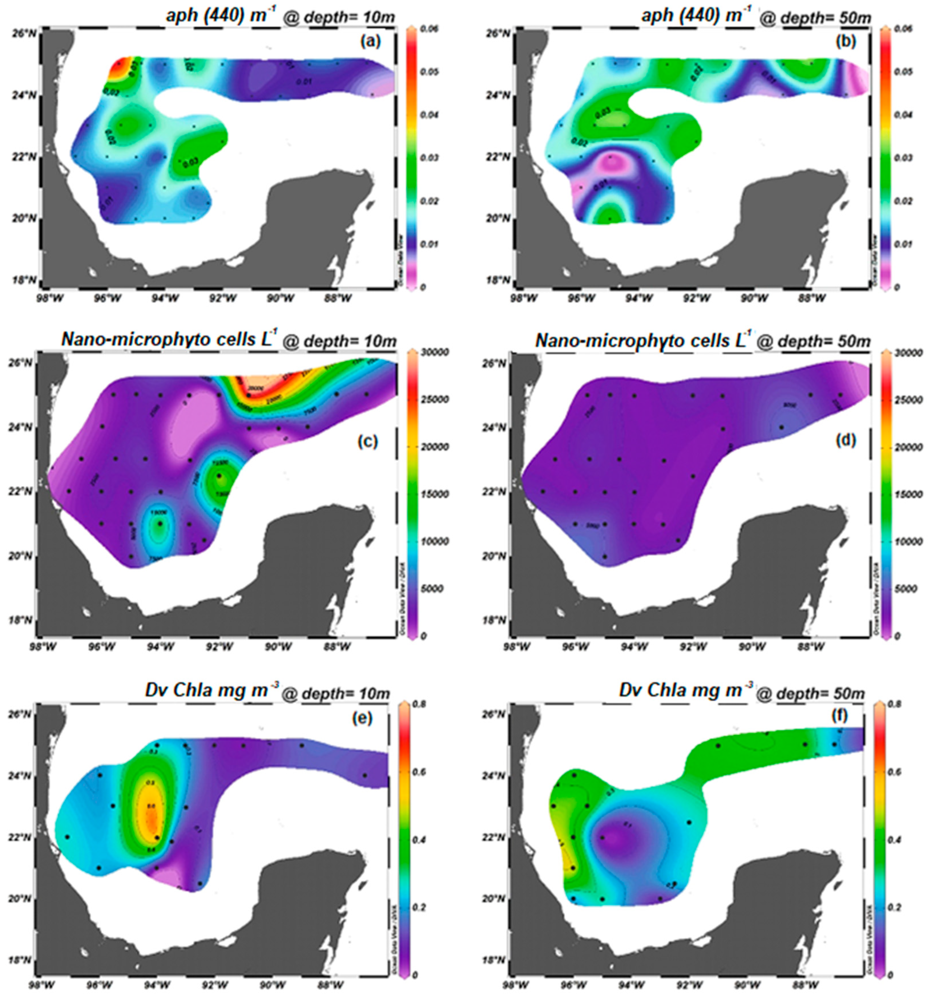
3.1.2. Bio-Optical Variability and Biogeochemical Conditions

Chlorophyll a. At the surface level, the spatial variability of Chla showed values that ranged from 0.07–0.63 mg m⁻³, with two well-defined areas: the southern and eastern regions of the GM had low Chla values, with an average of 0.12 mg m⁻³, whereas station E15 had a high concentration of 0.65 mg m⁻³ (Figure 3a). At the deep level, Chla values ranged from 0.06–0.69 mg m⁻³, and the spatial distribution was more mixed than that observed at the surface level. The highest Chla values were detected at the distant stations E23, E3B, and E40, with concentrations of 0.69, 0.65, and 0.56 mg m⁻³, respectively (Figure 3b). Phytoplankton absorption coefficient. At the surface level, a_ph values varied spatially and ranged between 0.006 to 0.055 m⁻¹, with two well-defined a_ph440. The group of stations with low a_ph440 values had an average of 0.01 m⁻¹; these stations were observed in the eastern and southwestern regions of the GM. The highest value (0.05 m⁻¹) was detected at station E15, off the Tamaulipas Shelf (Figure 3c, Table 1). In the deep layer, the spatial distribution of a_ph440 showed values that ranged between 0.002–0.031 m⁻¹, with the highest values recorded in the northeastern and southwestern regions of the GM at stations E3, E23, and E40, which showed values of up to 0.03 m⁻¹ (Figure 3d). Detritus absorption coefficient. At the surface level, a_d350 nm values ranged from 0.006–0.114 m⁻¹, with high values observed at stations E1 and E15, off the Tuxpan and San Fernando Rivers, respectively (Table 1). At the deep level, a_d350 values ranged from 0.006–0.047 m⁻¹ (Table 1), with the highest values recorded at stations E2, E3, and E3B located perpendicular to the coast at 23° N off the Tamaulipas Shelf. In general, the highest detritus values in the deep layer were approximately 41% lower than those on the surface layer. Nano-microphytoplankton abundance. In the surface level, the spatial variability of phytoplankton showed values that ranged from 826–27,910 cells L⁻¹ (Figure 3c,d, Table 1) and two well-defined areas: high abundance values were observed at stations E20, E23, and E30 in the northeast and stations E37, E40, and E47 in the southern region of the GM, with an average of 16,505 cells L⁻¹; the rest of the stations had an average of 2300 cells L⁻¹. In the deep level, abundance values of phytoplankton ranged from 138–6327 cells L⁻¹; high values were observed at stations E23, E30, and E40, with an average of 4356 cells L⁻¹ (Table 1). It is worth mentioning that stations E20, E47, and E37 showed a phytoplankton community dominance of cyanobacteria Oscillatoria sp. of 98%, 97%, and 90%, respectively (Figure 3c).

3.1.3. Spatial Distribution of Pigments

We report the spatial distribution of the three main pigments detected at each station. Divinyl chlorophyll a. On the surface level, DVchla ranged from 0.03–0.61 mg m⁻³ and showed two well-defined areas: in the central western region of the GM, station E7 showed high DVchla, located mainly in the central and eastern regions of the GM; the rest of the stations showed values < 0.15 mg m⁻³ (Figure 3e,

Table 2. HPLC-pigments (mg m⁻³) of the samples collected at two depth levels (10 and 50 m) in the CSWGM region from 19 February to 10 March 2013. Divinyl chlorophyll a (DVchla), chlorophyll b (Chlb), zeaxanthin (Zea), and 19′-Hexanoyloxyfucoxanthin (Hex-fuca).

Stations				Stations
10 m				50 m
Sta.-1	(mg m−3)	Sta.-22	(mg m−3)	Sta.-2	(mg m−3)	Sta.-35	(mg m−3)
DV chla	0.262	DV chla	0.145	DV chla	0.446	DV chla	0.232
Chlb	0.081	Zea	0.076	Chlb	0.079	Zea	0.060
Zea	0.064	Hex-fuco	0.013	Zea	0.069	Hex-fuco	0.024
Sta.-3b		Sta.-27		Sta.-3b		Sta.-39
DV chla	0.231	DV chla	0.118	DV chla	0.408	DV chla	0.504
Chlb	0.160	Zea	0.065	Chlb	0.231	Chlb	0.110
Hex-fuco	0.048	Hex-fuco	0.009	Hex-fuco	0.074	Zea	0.058
Sta.-7		Sta.-35		Sta.-4		Sta.-40
Chlb	0.761	DV chla	0.158	DV chla	0.410	Chlb	0.360
DV chla	0.606	Zea	0.040	Zea	0.063	DV chla	0.299
Hex-fuco	0.081	Chlb	0.040	Hex-fuco	0.050	Hex-fuco	0.046
Sta.-12		Sta.-37		Sta.-5		Sta.-42
Dvchla	0.202	DV chla	0.039	DV chla	0.039	DV chla	0.095
Chlb	0.087	Hex-fuco	0.009	Hex-fuco	0.009	Zea	0.058
Hex-fuco	0.006	Zea	0.006	Zea	0.006	Hex-fuco	0.018
Sta.-17		Sta.-39		Sta.-12		Sta.-46
DV chla	0.250	DV chla	0.225	DV chla	0.358	DV chla	0.218
Chlb	0.086	Zea	0.051	Chlb	0.208	Chlb	0.077
Zea	0.067	Chlb	0.051	Zea	0.062	Zea	0.028
Sta.-18		Sta.-43		Sta.-20		Sta.-47
DV chla	0.208	DV	0.153	DV chla	0.388	Chlb	0.268
Chlb	0.164	Zea	0.098	Chlb	0.146	DV chla	0.258
Zea	0.153	Chlb	0.092	Hex-fuco	0.050	Hex-fuco	0.024
Sta.-19		Sta.-44		Sta.-23
DVchla	0.091	DV chla	0.168	Chlb	0.475
Zea	0.058	Chlb	0.13	DV chla	0.357
Hex-fuco	0.008	Zea	0.009	Hex-fuco	0.168
Sta.-20				Sta.-24
DV chla	0.063			DV chla	0.213
Zea	0.049			Chlb	0.066
Hex-fuco	0.008			Hex-fuco	0.005

). At the deep level, the spatial distribution of the DVchla showed values that ranged from 0.03 to 0.51 mg m⁻³, with high concentrations at station E39 (Figure 3f, Table 2). Chlorophyll b. At the surface level, the spatial distribution of Chlb showed values that ranged from 0.04–0.76 mg m⁻³, with the highest value at station E7; the rest of the stations showed an average of 0.07 mg m⁻³ (Table 2). The deep level showed a range of values between 0.07–0.48 mg m⁻³, with high values at stations E23 and E40 (Table 2). Zeaxanthin. On the surface level, the spatial distribution of Zea showed values that ranged from 0.006–0.15 mg m⁻³, with the highest value at station E18; the rest of the stations showed an average of 0.06 mg m⁻³ (Table 2). The deep level showed Zea values that ranged from 0.006–0.07 mg m⁻³, with low values of 0.05 mg m⁻³ throughout the stations of the GM (Table 2). 19′-Hexanoyloxyfucoxanthin. At the surface level, the spatial distribution of Hex-fuco showed values that ranged from 0.006–0.08 mg m⁻³, with the highest value at station E7; the rest of the stations showed an average of 0.02 mg m⁻³ (Table 2). At the deep level, Hex-fuco values ranged from 0.005–0.17 mg m⁻³, with the highest value at station E23, whereas the rest of the stations showed an average of 0.03 mg m⁻³ throughout the station of the GM (Table 2).

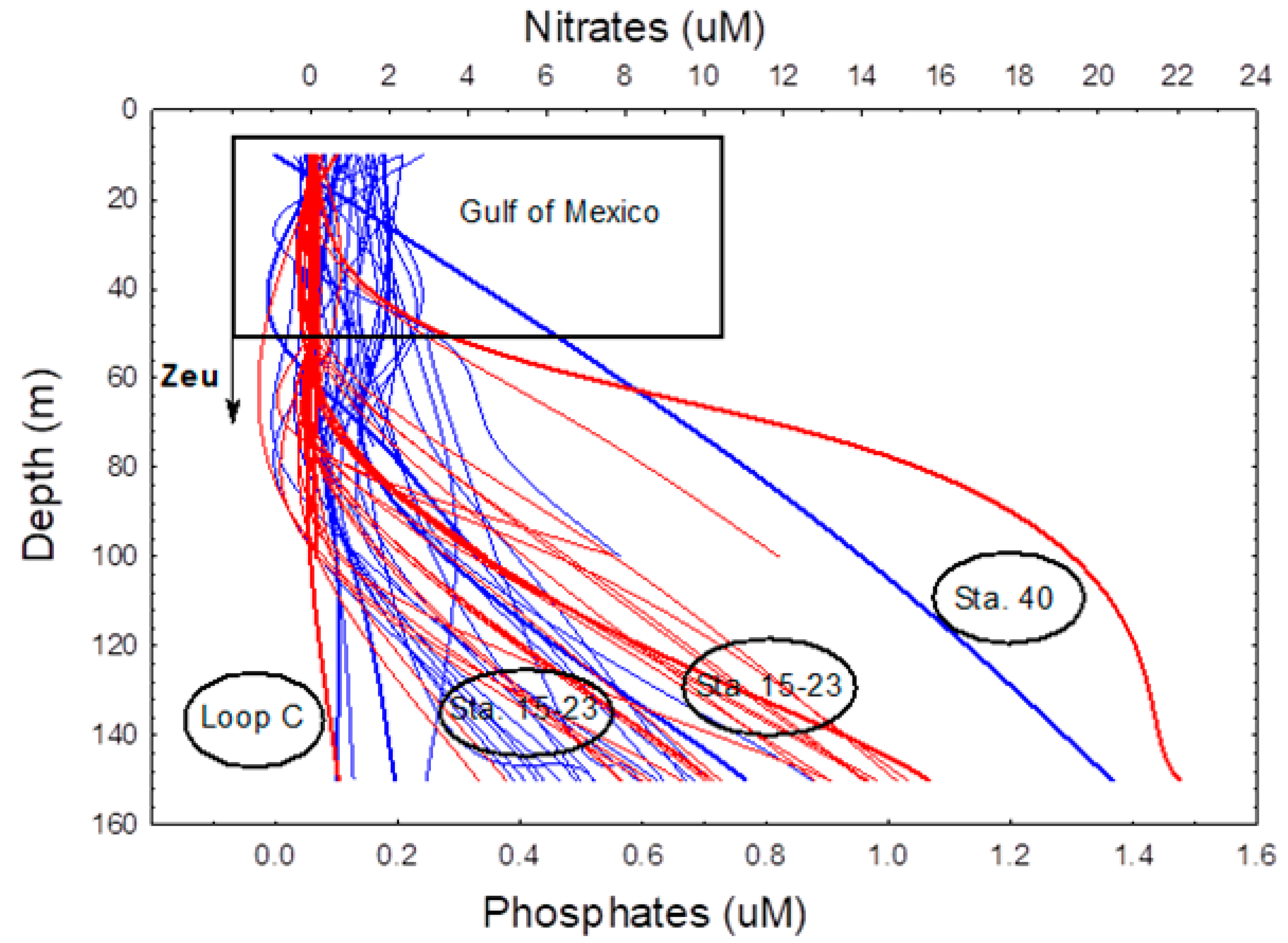
3.1.4. Spatial Distribution of Inorganic Nutrients

Nitrates and nitrites. At the surface level, the spatial distribution of NO₃⁻ showed values that ranged from 0.02–0.66 µM, with the highest values at stations E1, E30, and E44, whereas the rest of the stations showed an average of 0.09 µM (Figure 4, Table 1). At the deep level, NO₃⁻ values ranged between 0.03–3.37 µM, with the highest values at stations E40, E23, and E30; the rest of the stations showed an average of 0.09 µM throughout the stations of the GM (Figure 4, Table 1). Phosphates. At the surface level, the spatial distribution of HPO₄²⁻ showed values that ranged from 0.03–0.79 µM, with the highest values at stations E44 and E36; the rest of the stations showed an average of 0.13 µM (Figure 4). At the deep level, HPO₄²⁻ values ranged between 0.02–0.25 µM, with the highest values at stations E41, E17, and E43; the rest of the stations showed an average of 0.13 µM throughout the stations of the GM (Figure 4). Silicic acid. At the surface level, the spatial distribution of Si(OH)₄ showed values between 1.30–3.56 µM, with the highest values at stations E41 and E24, whereas the rest of the stations showed an average of 2.21 µM (no data shown). Values in the deep level ranged from 1.35–2.77 µM, with the highest value at station E41, whereas the rest of the stations showed an average of 2.13 µM throughout the stations of the GM.

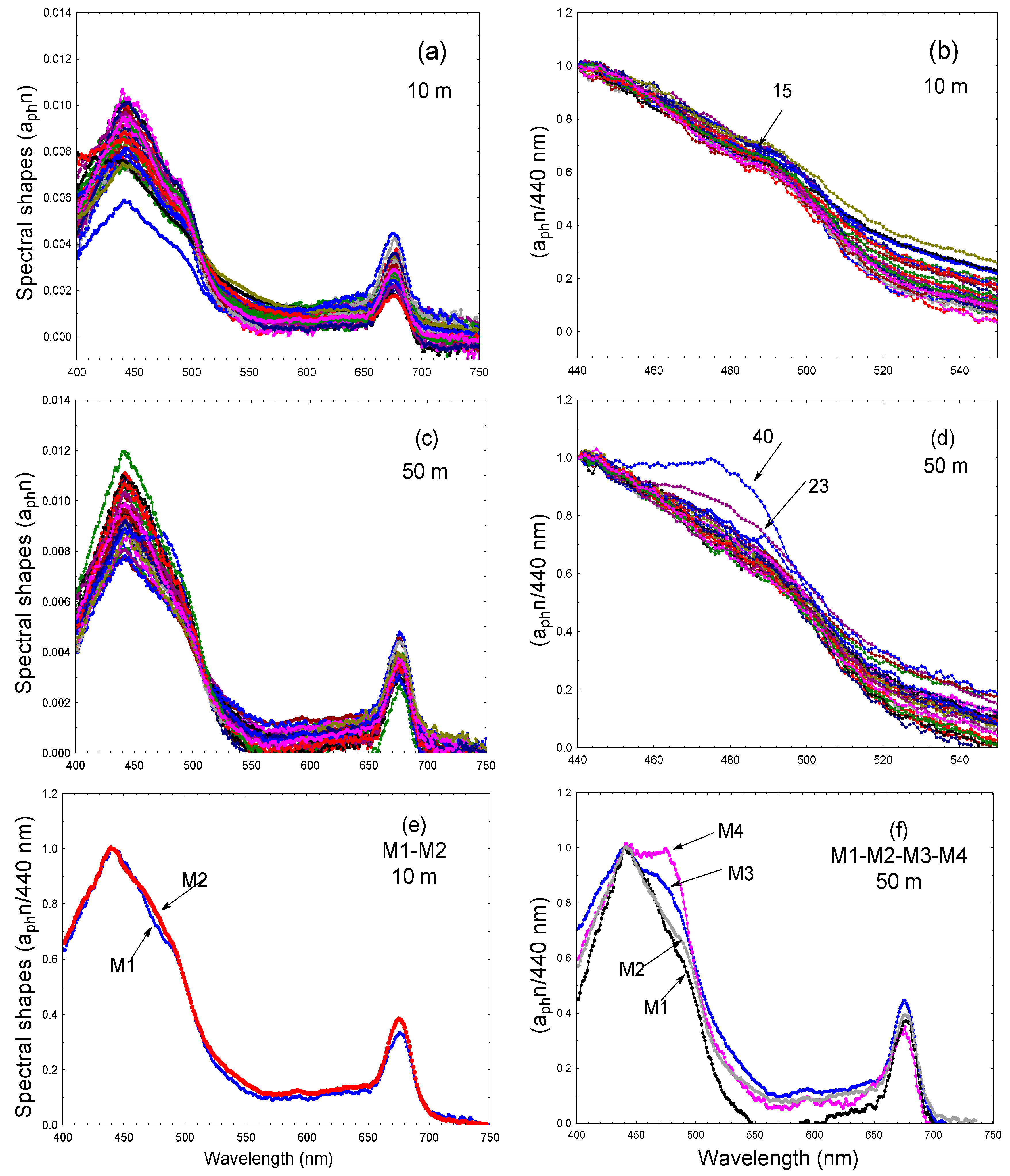
3.1.5. Phytoplankton Spectral Shapes

In this study, we analyzed a total of 56 normalized spectral curves (a_phn) corresponding to 33 curves on the surface and 23 in the deep level (Figure 5a,c). Subsequently, differences in slopes of curves between 440–550 (λ) were analyzed through cluster analysis [19] (Figure 5b,d). On the surface level, the a_phn/440 nm data showed slight differences and were classified into two spectral shapes named M1 and M2 (Figure 5e). In addition to the spectral shapes M1 and M2, the deep level showed two different shapes, named M3 and M4, at stations E23 and E40, respectively (Figure 5f). Ecological geography of phytoplankton. A total of four different phytoplankton spectral shapes (a_phn/440 nm) were reported for the CSWGM region. At the surface level, we detected the spectral shapes M1 and M2, with M1 dominating 85% of the area; conversely, M2 was detected only at five stations: E3, E3B, E15, E37, and E47 (Figure 6a). In the deep level, apart from M1 and M2, M3 and M4 (Figure 6b). The spectral shape M3 was detected at station E23, whereas M4 was detected at station E4.

4. Discussion

4.1. Oceanographic Conditions in the Gulf of Mexico

Elementary oceanographic information of GM has been reported since the 1930s, with conclusions showing considerable influence from the LC system. At present, it is known that the variability in the LC system largely depends on processes that control the shedding of large anticyclonic LC eddies (LCEs) from a northward elongated LC [3]; the LCEs subsequently travel westward into the GM, and the LC moves southward to a retracted position [3]. During February-March 2013, the western region of the GM was characterized by the presence of two anticyclonic structures [23]. These structures were remnants of the Jumbo anticyclone that was liberated from the LC during July 2012 and published in https://www.horizonmarine.com/loop-current-eddies.html. The hydrographic data in this study consolidates the historical 1930s results that the GM is affected by the presence and proximity of the LC system. Likewise, the spatial variability of low nutrients and high temperature-salinity (Figure 4 and Figure 7), and the T-S diagram in the data report from XIXIMI-3 corroborated the presence of two water masses: Caribbean Surface Water mass and the Gulf Common Water [23,24]. Our light penetration results using the Secchi disc ([9], Table 1) indicate that the average values of the euphotic zone (Zeu) extended to a depth of up to 72 m. Therefore, the 10 and 50 m depth levels are within the euphotic zone.

4.1.1. Phytoplankton and Absorption Properties

In general, the spatial distribution between Chla and Phyto in the CSWGM region did not present significant correlations. However, the high concentration (mg m⁻³) and abundances (cells L⁻¹) at stations E15, E23, and E40 resulted in different spectral shapes of a_phn/440 nm in relation to the rest of the stations (Figure 5b,d,f). Characteristically, these three stations showed higher water densities, with Sigma-t values above 25 kg m⁻³ (Table 1). Therefore, we can deduce that, in some areas of the CSWGM region, there were mixing processes in the water column with considerable nutrient input to the surface, as observed at stations E15 and E18 with an increase in HPO₄²⁻ up to 0.17 and 0.20 µM, respectively (Figure 4). The HPO₄²⁻ values were much lower than those reported for the Gulf of California [25], with both the Gulf of Mexico and the Gulf of California coinciding in the total consumption of NO₃⁻ for the surface level [25].

High values of non-pigmented particulate detrital material (a_d) were detected at stations E1 and E15 for the CSWGM region as a consequence of an increase in particulate organic matter inputs from the San Fernando and Tuxpan Rivers that flow into the Tamaulipas Shelf. Our detritus values for the stations nearest the coast were close to those reported for the Mississippi River mouth [13]. The absorption blue/red ratio (B/R) in the literature is suggested to determine phytoplankton size class distributions [26,27]. Our results showed that the optical properties at station E15, at 50 m depth, had a value of 1.86 B/R, corresponding to phytoplankton cell sizes of 9–27 µm, these optical values were similar to those reported during the Fall of 1999 in the northeastern Gulf of Mexico [13]. Previous studies on B/R ratios have shown that values below 2 correspond to large phytoplankton cell populations, as detected at station E15 with the presence of Tripos fusus (Ehrenberg) F. Gòmez, 2013, Gymnodinium spp., and Oxytoxum sp. In general, our values of the B/R ratio are similar to those obtained for the southern California Current, the northern South China Sea [26,27], and the northeastern Gulf of Mexico [13]. However, we consider that the B/R ratio in relation to the phytoplankton community has not yet been explored in detail.

Station E40, located in the coastal zone off Campeche Bay, was influenced by three large rivers (Figure 1). This station showed a spectral shape (M4) that differed from those of other stations in the GM (Figure 5f); we consider that these differences were caused by the diversity, abundance, and pigment variability of the phytoplankton, as well as the oceanographic conditions associated with low temperature (21.93 °C), high NO₃⁻ (3.37 µM), and Sigma-t < 25.32 kg m⁻³ (Table 1). On the other hand, the station (E23) showed a different spectral shape (M3) and had higher phytoplankton abundance of up to 6300 cells L⁻¹; we consider that this enrichment of phytoplankton cells could have resulted from a mixing effect caused by the convergence of the Caribbean Water mass and the Gulf Common Water, since the decreasing energy produces a border fertilization that stimulates the growth of phytoplankton [28]. This border fertilization has been reported for the Gulf of Mexico [29] and Gulf of California [25]. Of the 4 different spectral shapes (Figure 5f), only M1 and M2 dominated up to 85% of the area (Figure 6a); these dominant spectral shapes were already reported throughout the year for the northeastern Gulf of Mexico region [13]. In general, our results for spectral shape M1 coincide with the surface spatial distribution of Prochlorococcus reported for the north-central region of GM during winter 2013 [30], coinciding with low nano-microphytoplankton values (Table 1), which could be considered the Prochlorococcus as representative of the surface oligotrophic regions. Similarly, these authors [30] reported for the station E47 a homogeneous distribution of Synechococcus until 74 m (Table 1), corresponding these high biomass values with the spectral shape M2 of our study. Therefore, we could consider that the spectral shapes M1 and M2 correspond to groups of cyanobacteria such as Prochlorococcus and Synechococcus, respectively.

4.1.2. Optical Properties and Phytoplankton Pigments

The pigments PSC and PPC act in the process of photosynthesis and photoprotection, respectively. In our study, PSC pigments showed a greater spatial trend than PPC carotenoids (Table 2), with higher DVchla pigment dominating over Chlb, Hex-fuco, and Zea. We compared our PPC pigments with those reported for the southern California Current during El Niño 2002 [27] and observed a three-fold increase in the values for the CSWGM region. A high relationship was observed between our result of the pigment DVchla and the cyanobacterium Prochlorococcus, reported for the central GM region during the winter of 2013 [30]. Based on our pigment results, we deduce that the phytoplankton community structure in the Gulf of Mexico was dominated, in order, by Prochlorococcus, chlorophytes, prymnesiophytes, and Synechococcus.

5. Conclusions

Our results based on the variability of the bio-optical phytoplankton spectral shapes (a_phn/440 nm) showed that it was a suitable technique to delimit geographic ecological boundaries of phytoplankton in the Gulf of Mexico. In this study, we detected 4 spectral shapes with biomarker characteristics that represent large taxonomic groups of the phytoplankton community.

The ecological geography M1 and M2 dominated the surface level up to 85% of the area, with major pigments such as DVchla and zeaxanthin. Therefore, we could conclude that these spectral shapes correspond to groups of cyanobacteria such as Prochlorococcus and Synechococcus, respectively.

The stations E23 and E40, spatially separated among the other stations, marked differences between the biogeochemical processes in the GM. The station E40, located in the coastal zone off Campeche Bay, was influenced by three large rivers and showed an ecological geography (M4) that differed from those of other stations in the GM. We conclude that these differences were caused by the diversity, abundance, and pigment variability of the phytoplankton, produced through physical-biological interaction favorable to the phytoplankton community, associated with low temperature, high nutrients, and Sigma-t > 25. On the other hand, the station (E23) showed an ecological geography (M3) and had higher phytoplankton abundance; we consider that this enrichment of phytoplankton cells could have resulted from a mixing effect caused by the convergence of the Loop Current and the Gulf Common Water, since the decreasing energy produces a border fertilization that stimulates the growth of phytoplankton. Therefore, we could conclude that the ecological geography of M3 and M4 represents a mixture of diatoms, dinoflagellates, and chlorophytes.

Therefore, the importance of conducting holistic research gives us the opportunity for an interpretation as close to nature as possible.

References

1. Parr, A.E. Report on hydrographic observations in the Gulf of Mexico and the adyacent straits made during the Yale Oceanography Expedition on the Mabel Taylor in 1932. Bull. Bingham Ocean. 1935, 5, 1–93. [Google Scholar]
2. Leipper, D.F. Physical oceanography of the Gulf of Mexico. Fish. Bull. Fish Wildl. Serv. 1954, 55, 119–137. [Google Scholar]
3. Androulidakis, Y.; Kourafalou, V.; Olascoaga, M.J.; Berón-Vera, F.J.; Le Hénaff, M.; Kang, H.; Ntaganou, N. Impact of Caribbeans anticyclones on Loop Current variability. Ocean. Dyn. 2021, 71, 935–956. [Google Scholar] [CrossRef]
4. Weisberg, R.H.; Liu, Y. On the Loop Current penetration into the Gulf of Mexico. J. Geophys. Res.-Oceans 2017, 122, 9679–9694. [Google Scholar] [CrossRef]
5. Buenfil, J. Executive summary. In Adaptación a los Impactos del Cambio Climático en los Humedales Costeros del Golfo de México; Buenfil, J., Ed.; SEMARNAT: Mexico City, Mexico, 2009; pp. 25–34. [Google Scholar]
6. Pasqueron de Fommervault, O.; Pérez-Brunius, P.; Damien, P.; Camacho-Ibar, V.F.; Sheinbaum, J. Temporal variability of chlorophyll distribution in the Gulf of Mexico: Bio-optical data from profiling flots. Biogeosciences 2017, 14, 5647–5662. [Google Scholar] [CrossRef]
7. Yingling, N.; Thomas, K.B.; Shropshire, T.A.; Landry, M.R.; Selph, K.E.; Knapp, A.N.; Kranz, S.A.; Stukel, M.R. Taxon-specific phytoplankton growth, nutrient utilization and light limitation in the oligotrophic Gulf of Mexico. J. Plankton Res. 2022, 44, 656–676. [Google Scholar] [CrossRef]
8. Yentsch, C.S.; Phinney, D.A. A bridge between ocean optics and microbial ecology. Limnol. Oceanogr. 1989, 34, 1694–1705. [Google Scholar] [CrossRef]
9. Kirk, J.T.O. Light and Photosynthesis in Aquatic Ecosystems, 2nd ed.; Cambridge University Press: Cambridge, UK, 1994; p. 509. [Google Scholar]
10. Gieskes, W.W.C.; Kraay, G.W.; Nontji, A.; Setiapermana, D.; Sutomo, D. Monsoonal alteration of a mixed and a layered structure in the euphotic zone of the Banda Sea (Indonesia): A mathematical analysis of algal pigment fingerprints. Neth. J. Sea Res. 1988, 22, 123–137. [Google Scholar] [CrossRef]
11. Goericke, R.; Repeta, D.J. The pigments of Prochlorococcus marinus: The presence of divinyl chlorophyll a and b in a marine prokaryote. Limnol. Oceanogr. 1992, 37, 425–433. [Google Scholar] [CrossRef]
12. Sánchez-Pérez, E.D.; Millán-Núñez, E. Ecological zonation of phytoplankton and biomass based on bio-optical parameters off Baja California during three summer seasons. Open J. Mar. Sci. 2019, 9, 121–136. [Google Scholar] [CrossRef]
13. Nababan, B. Bio-Optical Variability of Surface Waters in the Northeastern Gulf of Mexico. Ph.D. Thesis, University of South Florida, Tampa, FL, USA, 2005. Available online: http://scholarcommons.usf.edu/etd/784 (accessed on 3 May 2005).
14. Damien, P.; Sheinbaum, J.; Pasqueron de Fommervault, O.; Jouanno, J.; Linacre, L.; Duteil, O. Do Loop Current Eddies stimulate productivity in the Gulf of Mexico. Biogeosciences 2021, 18, 4281–4303. [Google Scholar] [CrossRef]
15. Throndsen, J. Preservation and storage. In Phytoplankton Manual. Monographs on Oceanographic Methodology; Sournia, A., Ed.; UNESCO: Paris, France, 1978; Volume 6, pp. 69–74. [Google Scholar]
16. Holm-Hansen, O.; Lorenzen, C.; Holmes, R.; Strickland, J. Fluorimetric determination of chlorophyll. J. Mar. Sci. 1965, 30, 3–15. [Google Scholar] [CrossRef]
17. Van Heukelem, L.; Thomas, C. Computer assisted high-performance liquid chromatography method development with applications to the isolation and analysis of phytoplankton pigments. J. Chromatogr. A 2001, 910, 31–49. [Google Scholar] [CrossRef]
18. Cleveland, J.S.; Weidemann, A.D. Quantifying absorption by aquatic particles: A multiple scattering correction for glass- fiber filters. Limnol. Oceanogr. 1993, 38, 1321–1327. [Google Scholar] [CrossRef]
19. Millán-Núñez, E.; Macías-Carballo, M. Phytogeography associated at spectral absorption shapes in the southern region of the California Current. CalCOFI Rep. 2014, 55, 183–196. [Google Scholar]
20. Hasle, G.R. The inverted-microscope method. In Phytoplankton Manual; Sournia, A., Ed.; United Nations Educational, Scientific and Cultural Organization: Paris, France, 1978; Volume 5.2.1, p. 337. [Google Scholar]
21. Tomas, C.S. Identifying Marine Phytoplankton; Academic Press, Inc.: New York, NY, USA, 1997; p. 345. [Google Scholar]
22. Gordon, L.I.; Jennings, J.C., Jr.; Ross, A.A.; Krest, J.M. A suggested protocol for continuous flow automated analysis of seawater nutrients (phosphate, nitrate, nitrite and silicie acid) in the WOCE Hydrographic Program and the Joint Global Ocean Fluxes Study. In Methods Manual WHPO: Oregon State University College of Oceanography; WOCE Hydrographic Program Office, 1993; pp. 1–55. Available online: https://www2.whoi.edu/site/wp-content/uploads/sites/84/2019/07/gordnut_133885.pdf (accessed on 3 May 2025).
23. García-Córdova, J.; Sheinbaum, J. Hidrografía y Condiciones Físicas, CTD (Temperatura, Salinidad, O2, Fluorescencia, Clorofila-a). In: Monitoreo Ambiental en Aguas Profundas del Golfo de México en Respuesta al Derrame Petrolero Asociado a la Plataforma Deepwater Horizon. Informe Final. 2014, p. 447. Available online: https://www.gob.mx/cms/uploads/attachment/file/344074/CGACC_2014_XIXIMI_3_CICESE_PARTE1.pdf (accessed on 3 May 2025).
24. Quintanilla, J.G.; Herguera, J.C.; Sheinbaum, J. Oxygenation of the Gulf of Mexico thermocline linked to the detachment of Loop Current eddies. Front. Mar. Sci. 2024, 11, 1479837. [Google Scholar] [CrossRef]
25. Millán-Núñez, E.; Delgadillo-Hinojosa, F.; Hakspiel-Segura, C.; Torres-Delgado, E.V.; Félix-Bermudez, A.; Segovia-Zavala, J.A.; Camacho-Ibar, V.F.; Muñoz-Barbosa, A. Phytoplankton composition and biomass under oligotrophic conditions in the Guaymas Basin (Gulf of California). Cienc. Mar. 2023, 49, 1–15. [Google Scholar] [CrossRef]
26. Wu, J.; Hong, H.; Shang, S.; Dai, M.; Jee, Z. Variation of phytoplankton absorption coefficients in the northern South China Sea during spring and autumn. Biogeosci. Discuss. 2007, 4, 1555–1584. [Google Scholar]
27. Millán-Núñez, E.; Millán-Núñez, R. Specific Absorption Coefficient and Phytoplankton Community Structure in the Southern Region of the California Current during January 2002. J. Oceanogr. 2010, 66, 719–730. [Google Scholar] [CrossRef]
28. Mann, K.H.; Lazier, J.R. Dinamics of Marine Ecosystems: Biological-Physical Interactions in the Oceans; Blackwell: Oxford, UK, 1991; p. 466. [Google Scholar]
29. Aldeco, J.; Monreal-Gómez, M.A.; Signoret, M.; Salas-de León, D.A.; Hernández-Becerril, D.U. Ocurrence of a subsurface anticyclonic eddy, fronts, and Trichodesmium spp. over the Campeche Canyon region, Gulf of México. Cienc. Mar. 2009, 35, 333–344. [Google Scholar] [CrossRef]
30. Linacre, L.; Lara-Lara, R.; Camacho-Ibar, V.; Herguera, J.C.; Bazán-Guzmán, C.; Ferreira-Bartrina, V. Distribution pattern of picoplankton carbon biomass linked to mesoscale dynamics in the southern gulf of Mexico during winter conditions. Deep.-Sea Res. I 2015, 106, 55–67. [Google Scholar] [CrossRef]
Figure 1. Station locations in the central southwestern Gulf of Mexico (CSWGM) during the XIXIMI-3 cruise carried out from 19 February to 10 March 2013. The deep contours are distinguished from the coastal ocean by 200 and 1000 m. The major river discharges at the Tamaulipas Shelf (San Fernando and Tuxpan) and Campeche Bay (Coatzacoalcos and Usumacinta). The subset marks the location of the GM.
Jmse 13 01128 g001
Figure 2. Spatial distribution at two depth levels (10 and 50 m) in the CWGM region. Temperature (a,b), salinity (c,d), and chlorophyll a (e,f). The black dots represent sampling stations.
Jmse 13 01128 g002
Figure 3. Spatial distribution at two depth levels (10 and 50 m). Phytoplankton absorption coefficient (a,b), nano-microphytoplankton (c,d), and divinyl chlorophyll a (e,f). The black dots represent sampling stations.
Jmse 13 01128 g003
Figure 4. Spatial distribution of the nutrients (nitrates and phosphates) up to 150 m. The black rectangle and ellipses contain the main stations of the Loop Current and Gulf of Mexico. Average value of the euphotic zone (Zeu). Nitrates color red, and phosphates color blue.
Jmse 13 01128 g004
Figure 5. Phytoplankton spectral shapes normalized at two depth levels (10 and 50 m), the stations of the spectral curves (a,c) are represented by colors. Spectral shapes aphn (a,c), spectral shapes between 440–550 nm aphn/440 (b,d). Mean spectral shapes at 10 m M1–M2 (e) and mean spectral shapes at 50 m M1–M2 and M3–M4 (f).
Jmse 13 01128 g005
Figure 6. Ecological geography of the phytoplankton at two depth levels (10 and 50 m) is represented by different colors: (a) green (M1), red (M2), and (b) green (M1), red (M2), yellow (M3), orange (M4).
Jmse 13 01128 g006
Figure 7. Spatial distribution of the temperature and salinity up to 150 m. The black rectangle and ellipses contain the main stations of the Loop Current and Gulf of Mexico. Average value of the euphotic zone (Zeu). Temperature color red and salinity color green.
Jmse 13 01128 g007