Motion Control of a Flexible-Towed Underwater Vehicle Based on Dual-Winch Differential Tension Coordination Control

Abstract

This paper focused on the motion control of an underwater vehicle installed on a linear guide system, which is driven by two electric winches with wire ropes. The vehicle is subject to complex nonlinear time-varying disturbances and actuator input saturation effects during motion. A coupled dynamic model, incorporating an underwater vehicle, winches, and wire ropes, was established. Particular attention was paid to the nonlinear time-varying hydrodynamic disturbances acting on the underwater vehicle. The Kelvin–Voigt model was introduced to characterize the nonlinear dynamic behavior of the wire ropes, enabling the model to capture the dynamic response characteristics of traction forces. To tackle cross-coupling within the towing system, a differential tension coordination control method was proposed that simultaneously regulates system tension during motion control. For the vehicle dynamics model, a nonsingular fast-terminal sliding-mode (NFTSM) controller was designed to achieve high-precision position tracking control. An auxiliary dynamic compensator was incorporated to mitigate the impact of actuator input saturation. To handle time-varying disturbances, a fuzzy adaptive nonlinear disturbance observer (FANDO) is developed to perform feedforward compensation. Stability proof of the proposed algorithms was provided. Extensive numerical simulations demonstrate the effectiveness of the control strategies. Compared to the NFTSM without the disturbance observer the absolute mean value of the tracking error decreased by 76%, the absolute maximum value of the tracking error decreased by 67%, and the mean square error decreased by 93.5%.

1. Introduction

With the over-exploitation and gradual depletion of terrestrial resources, marine resource exploration has increasingly become a major focus of international research over the past two decades. However, it continues to face significant challenges due to the complexity of the underwater environment and the lack of essential observation and communication technologies. Notably, intelligent underwater equipment can substantially reduce the costs and risks associated with various underwater missions [1], which has led to a growing demand for high-precision underwater operational capabilities, thereby driving technological innovations in next-generation marine systems.

The underwater vehicle investigated in this study is primarily designed to provide a stable dynamic testing platform for onboard submerged equipment. The experimental requirements of the equipment necessitate that the vehicle executes stable and high-precision motions. This operational demand has driven the implementation of a unique structural configuration in its design. The vehicle’s main body is cylindrical and mounted on a linear guidance system. The linear guidance system ensures complete lateral motion restraint of the vehicle. The towing system consists of two motor-driven winches and their respective steel wire ropes. The dual-cable traction system effectively mitigates flow-induced disturbance issues inherent in conventional thruster systems. The vehicle moves along a linear guide rail to perform precise trajectory tracking, including accelerated startup, constant-speed cruising, and smooth braking. These maneuvers must be executed within the finite stroke of the guide rail, providing a stable dynamic testing platform for onboard, submerged equipment. Research on motion control strategies for this underwater vehicle is expected to provide methodological references for dual-motor drive systems in other domains.

Existing underwater motion control systems face two challenges when applied to these underwater vehicles:

(1)

Coordinated control of the dual-winch towing system with dual-actuator input saturation constraints.

(2)

High-precision position tracking control of the underwater vehicle under nonlinear time-varying disturbances.

1.1. Literature Review

(1)

Dual-Motor Coordination Control

The primary challenges in coordinated control lie in regulating dual-winch outputs to ensure the system can both generate precise driving forces required for vehicle motion and simultaneously mitigate tension chattering in the wire ropes while avoiding actuator saturation. For high-precision position tracking control, the core difficulty resides in enabling the underwater vehicle to achieve rapid convergence to reference trajectories and maintain precise trajectories following nonlinear time-varying disturbances.

Current dual-motor coordination control strategies mainly include master–slave synchronous control and force–position decoupled control. In master–slave synchronous control, one motor is designated as the master, and the other as the slave. The master motor’s motion states (e.g., position, velocity, acceleration) are transmitted as reference signals to the slave motor in real time via high-speed communication. Upon receiving these signals, the slave motor adjusts its motion using predefined control algorithms (e.g., master–slave control, cross-coupled control [2]) to achieve precise synchronization. Sun Chungeng et al. proposed a cross-coupled sliding-mode synchronous control method for dual-lift-point hydraulic elevators, incorporating both single-cylinder tracking errors and dual-cylinder synchronous errors. This approach achieves 53.1% higher synchronization accuracy during the initial phase compared to proportional-derivative (PD) cross-coupled synchronization, while attaining a 90% improvement in steady-state synchronization precision [3]. Ying Mu et al. proposed integration of average speed and sub-average speed to optimize the speed compensator. This integration mitigated speed synchronization errors, minimized synchronization adjustment time, and elevated overall system synchronization performance [4]. Ziqi Zhou et al. proposed a variable error difference compensation-coupling control (VEDC-CC) strategy to achieve precise cooperative control of dual motors in rudderless dual-motor propelled vessels. This method enables mutual coupling of self-errors and effectively enhances cooperative control performance under various command inputs [5]. In force–position decoupled control, the two motors independently handle motion control and tension regulation. Specifically, the motor on the vehicle’s motion direction front governs trajectory tracking (position control), while the motor on the rear regulates the towing system’s tension (force control). This method provides an effective solution for eliminating tracking errors in engineering applications [6,7]. However, since tension and position are controlled by separate motors, frequent direction reversals force continuous switching between control modes, leading to significant performance degradation. Mitsantisuk et al. proposed a dual direct-drive motor towing structure [8], which adjusts system stiffness by modulating cable pre-tension to ensure operator safety in human–robot interactions. They identified that tracking errors primarily stem from friction at low speeds and inertial forces at high speeds [9]. To address this, they developed a variable cable tension strategy: low cable stiffness during low-speed motion to absorb disturbances and high stiffness during high-speed motion to suppress oscillations. This research prioritizes human–robot interaction compliance over positioning accuracy.

(2)

Dynamic position tracking control

Dynamic position tracking control under complex disturbances presents another critical challenge. The underwater vehicle and its towing system form a multivariable, strongly coupled, and nonlinear system, where conventional PID control fails to meet high-performance requirements when subjected to external uncertainties. To address this, extensive research has led to the successful application of modern control theories such as adaptive control, fuzzy control, neural networks, and active disturbance rejection control. Sliding-mode control (SMC), in particular, has gained increasing attention due to its low dependency on model accuracy and strong robustness against parameter variations and external disturbances [10], making it highly effective for managing the nonlinearities and uncertainties inherent in such coupled systems.

Sliding-mode control (SMC) is inherently a class of nonlinear control characterized by discontinuous control actions. Unlike conventional control strategies, SMC dynamically alters the system’s “structure” based on real-time states (e.g., tracking errors and their derivatives) to enforce predefined “sliding-mode” trajectories. Theoretically, SMC ensures finite-time convergence to the sliding surface for systems with bounded uncertainties and disturbances. If uncertainties and disturbances satisfy matching conditions, the sliding mode exhibits complete invariance to them, offering strong robustness and making SMC a powerful approach for time-varying uncertain systems. However, in practical applications, the system state cannot perfectly remain on the sliding surface due to inherent inertia in the switching control law, resulting in the chattering phenomenon—high-frequency oscillations across the sliding surface. Chattering degrades dynamic performance (e.g., overshoot, instability) and accelerates mechanical wear. Yin X. et al. presents a method of designing a small switching gain based on the estimation error. Combining the SMC, the EID approach, and the switching-gain design law, they present a new system configuration. The presented SMC-based EID control system not only improves the disturbance-suppression performance of the EID approach but also solves the chattering problem in the SMC [11]. To enhance the convergence rate of state errors and mitigate chattering effects, Bharti R.R. and Santosha K.D. proposed an adaptive nonsingular fast-terminal sliding-mode (NFTSMC) control scheme incorporating a piecewise fast multi-power reaching law. By leveraging the advantages of the adaptation law, this method prevents overestimation of control parameters and eliminates the requirement for prior knowledge of disturbance upper bounds [12]. Advanced mechanisms have been integrated into SMC to enhance precision, including adaptive switching gain laws [13,14,15,16], time-delay estimators (TDEs) [11,17], and adaptive radial basis function neural networks (RBFNNs) [18,19,20,21]. To improve convergence rates of sliding variables, Man et al. proposed terminal sliding-mode control (TSMC), enabling finite-time convergence [22]. However, TSMC suffers from singularity issues in control inputs, which were later resolved via nonsingular terminal SMC (NTSMC) [23,24,25]. Martinez-Perez et al. developed an adaptive nonsingular terminal sliding-mode trajectory-tracking controller for an unmanned underwater vehicle subject to disturbances. The nonsingular terminal sliding-mode manifold ensures practical finite-time convergence of the tracking error to a neighborhood of zero [26].

To enhance control system performance, Yasutaka Fujimoto et al. proposed a combined controller integrating chattering-free sliding-mode control with disturbance observers [27]. Li Wenhua et al. proposed an active heave compensation control scheme for marine winches, integrating hybrid neural network prediction with a high-gain observer-based sliding-mode controller to significantly enhance control accuracy [28]. Liu et al. investigated backstepping finite-time SMC for underwater vehicle trajectory tracking, employing a nonlinear disturbance observer to mitigate uncertainties and external disturbances [29]. Sedghi et al. addressed the finite-time path-following control of autonomous underwater vehicles (AUVs) with saturated inputs and uncertainties [30]. In [31], Qiao and Zhang developed an adaptive second-order fast nonsingular TSMC scheme for AUVs, requiring no prior knowledge of system uncertainty bounds. Ali et al. introduced a finite-time extended-state observer-based nonsingular fast TSMC, achieving rapid finite-time stabilization [32]. Cui et al. further developed an auxiliary dynamic compensator for controlling actuator saturation in underwater vehicles.

While these methods provide valuable insights, two critical gaps remain when applied to our system:

(1)

Existing coordinated strategies have difficulty achieving tension–position coupling control.

(2)

There is a lack of integrated solutions for precise position control that simultaneously avoid saturation and suppress disturbances.

1.2. Research Focus

This paper focuses on the motion control of an underwater vehicle with a unique configuration. Inspired by the aforementioned research, this paper proposed a dual-motor differential tension coordinated control method based on nonsingular fast-terminal sliding-mode control and a fuzzy adaptive nonlinear disturbance observer. The method aims to achieve stable tension regulation and high-precision position tracking under time-varying nonlinear disturbances while satisfying actuator input saturation constraints.

The rest of this paper is organized as follows: Section 2 briefly introduces the structure and modeling of the dual-winch-towed underwater vehicle system. Section 3 presents the dual-motor differential tension coordinated control strategy and the nonsingular fast-terminal sliding-mode control method integrated with a fuzzy adaptive nonlinear disturbance observer. Section 4 provides the simulation results. Finally, Section 5 concludes the paper.

2. Modeling of Underwater Vehicles and Traction Systems

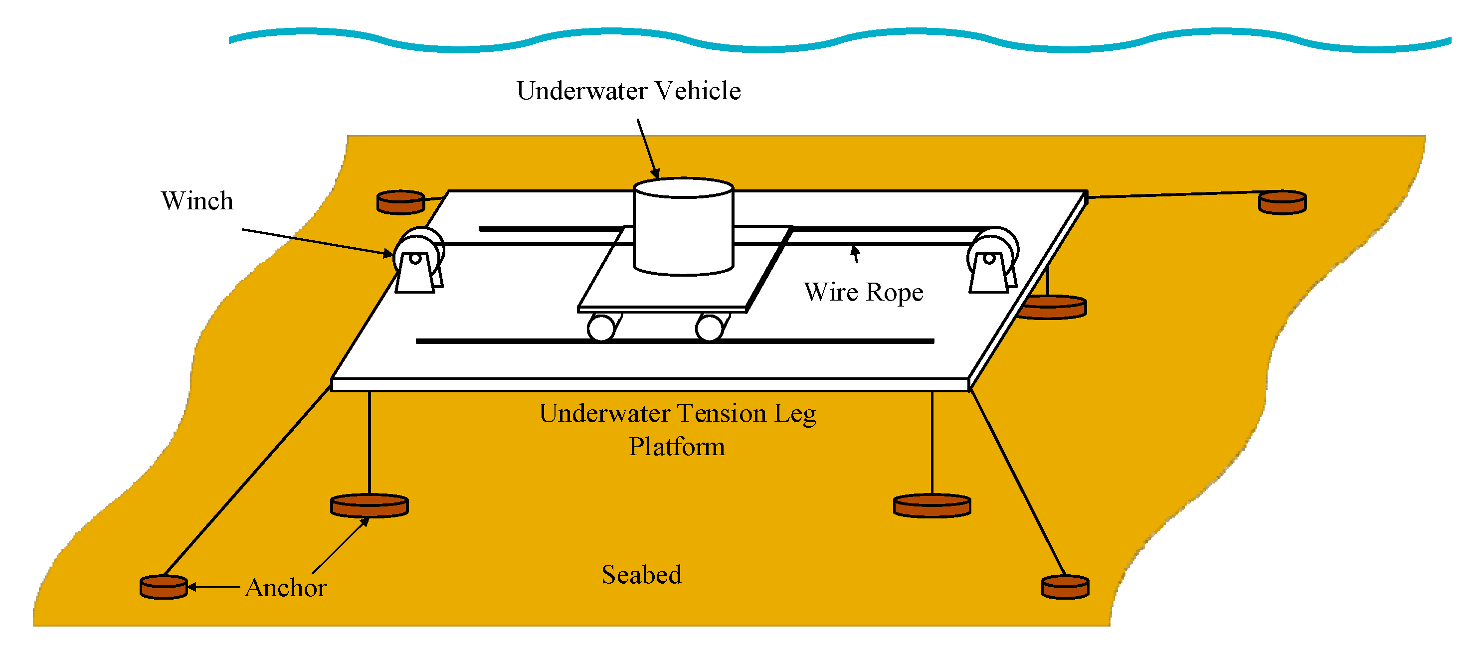
2.1. Structure of the System

The main body of the underwater vehicle is a cylindrical structure mounted on a linear guidance system. The vehicle is towed by two motor-driven winches via steel wire ropes. One end of each steel wire rope is securely fastened to the winch drum to prevent relative sliding, while the other end is connected to a plate–ring tension sensor and ultimately fixed to the underwater vehicle. The motors, coupled with the winch drums via coaxial shafts through gear reducers for speed reduction, are equipped with incremental encoders to measure motor rotational speed. A wheel-based speed-measurement device is installed on the vehicle to monitor its velocity relative to the guide rail. The entire system is mounted on an adjustable underwater platform that remains horizontal during vehicle motion. A schematic diagram of the underwater vehicle is shown in Figure 1.

2.2. Modeling of the Wire Rope

The wire ropes are connected between the winches and the underwater vehicle, transmitting the towing forces generated by the winches to the vehicle. The system employs high-strength alternate-lay wire ropes, with each wire rope being single-layer-wound and fixed on the winch drum at one end, while the other end is connected to the vehicle through a plate–ring load cell, as illustrated in Figure 2.

During the motion of the underwater vehicle, the control system adjusts the winch outputs to ensure the steel wire rope remains tensioned. Therefore, the Kelvin–Voigt model is employed to characterize the wire rope properties, neglecting the bending stiffness and radial deformation of the steel wire rope. Based on the kinematic relationship between the winch and the vehicle, the geometric condition between the wire rope retraction length and the vehicle displacement must be satisfied.

$$\Delta L=R\theta -x$$

(1)

where $\Delta L$ is the elastic elongation of the steel wire rope, $R$ is the radius of the winch drum, $\theta$ is the curvature of the winch drum rotation, and $x$ is the displacement of the aircraft. The derivative of $\Delta L$ can be written as:

$$\Delta \dot{L}=R\dot{\theta }-\dot{x}$$

(2)

Based on the Kelvin–Voigt model, the tension in the steel wire rope is composed of an elastic component and a viscous damping component. According to Hooke’s law, the elastic restoring force is linearly proportional to the elongation.

$$F_{elasticity}={\displaystyle \frac{EA}{L}}\left(R\theta -x\right)$$

(3)

where E is the equivalent axial elastic modulus of the steel wire rope, A is the cross-sectional area of the steel wire rope, and L is the initial length of the steel wire rope.

Considering internal material friction and inter-strand slippage energy dissipation in the steel wire rope, the damping force is proportional to the elongation rate.

$$F_{damping}=c\left(R\dot{\theta }-\dot{x}\right)$$

(4)

where c is the equivalent damping coefficient of the steel wire rope. The total tension of the steel wire rope can be written as follows:

$$F=F_{elasticity}+F_{damping}={\displaystyle \frac{EA}{L_0}}\left(R\theta -x\right)+c\left(R\dot{\theta }-\dot{x}\right)$$

(5)

where $L_0$ is the total length of the track. The underwater vehicle is in its initial position, $x=0$. At this time, the length of wire rope 1 is $L_0$, and the length of wire rope 2 is 0. Therefore, the tension on the two steel wire ropes is expressed as follows:

$$\left\{\begin{array}{c}{F}_1={\displaystyle \frac{EA}{L_o-x}}(R{\theta }_1-x)+c(R{\dot{\theta }}_1-\dot{x})\\ F_2={\displaystyle \frac{EA}{x}}(x-R{\theta }_2)+c(\dot{x}-R{\dot{\theta }}_2)\end{array}\right.$$

(6)

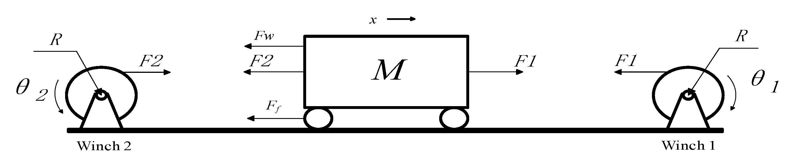
2.3. Modeling of the Underwater Vehicle

The underwater vehicle, which is approximately cylindrical in shape, operates under the constraint of a linear positioning system. When analyzing the hydrodynamic forces acting on the vehicle, these forces can be decomposed into two components: hydrodynamic resistance induced by the vehicle’s own motion, and hydrodynamic loads generated by ambient currents.

The resistance caused by the vehicle’s motion always opposes its direction of movement, whereas ambient currents may originate from arbitrary directions. Hydrographic observations in the experimental waters indicate that ambient current velocities typically remain below 0.3 knots (≈0.154 m/s), which is significantly small compared to the vehicle’s operational speed.

Assumption 1. 

The lateral hydrodynamic components induced by ambient currents can be effectively neutralized by the restoring force of the linear guidance system. Consequently, the ambient current effects are modeled as a stochastic disturbance superimposed on the primary hydrodynamic resistance with the following characteristics:

(a)

Directional randomness persists within the horizontal plane.

(b)

Temporal variations exhibit characteristic frequencies below the vehicle’s control bandwidth.

The resultant force experienced by the underwater vehicle during motion includes four parts; the tension, F₁, of wire rope 1; the tension, F₂, of wire rope 2; the frictional resistance, F_f; and the water resistance, F_w.

The force on the underwater vehicle is shown in Figure 3.

Based on Newton’s second law, the dynamic equation of the underwater vehicle can be obtained as follows:

$$F_1-F_2-F_f-F_w=M\ddot{x}$$

(7)

where F₁ and F₂ are the tension of wire rope 1 and wire rope 2, $F_f=\mu F_N=\mu ({\overline{F}}_N+\Delta )$ denotes the frictional resistance acting on the underwater vehicle, and $F_w={\displaystyle \frac{1}{2}}{C}_d\rho A{\dot{x}}^2$ denotes the hydrodynamic drag acting on the underwater vehicle.

After substitution, we can obtain:

$$M\ddot{x}={\displaystyle \frac{EA}{L_o-x}}(R{\theta }_1-x)+c(R{\dot{\theta }}_1-\dot{x})-{\displaystyle \frac{EA}{x}}(x-R{\theta }_2)+c(\dot{x}-R{\dot{\theta }}_2)-\mu ({\overline{F}}_N+\Delta )-{\displaystyle \frac{1}{2}}{C}_d\rho A_v{\dot{x}}^2$$

(8)

2.4. Modeling of the Winches

Each winch comprises a motor, a gearbox, and a drum. The steel wire rope is wound onto the winch drum in a single-layer helical configuration, ensuring no overlapping or cross-winding between adjacent turns. This design prevents concentrated compressive forces and inter-rope friction caused by multi-layer winding. Additionally, the single-layer arrangement establishes a linear relationship between the rope’s linear velocity and the drum’s rotational speed, enabling precise calculation of payout/retrieval length, reducing nonlinear errors from overlapping, and enhancing high-precision control.

To facilitate analysis, the rotational speed and torque in the wire rope retrieval direction are defined as positive for the winches. Specifically, winch 1 adopts clockwise rotation as its positive direction, while winch 2 uses counterclockwise rotation as the positive direction, as shown in Figure 2 and Figure 3. Clearly, given that the wire ropes can only transmit tensile forces, each winch’s torque output is constrained to positive values. This definition facilitates unified analysis of the winches’ input saturation constraints.

For winch 1:

$$I_1{\tau }_1-F_{1}R-{\tau }_{f1}=J_1{\ddot{\theta }}_1$$

(9)

where $I_1$ represents the transmission ratio, ${\tau }_1$ represents the torque output by the motor in winch 1, ${\tau }_{f1}$ represents the friction torque between the wire rope and winch 1, and $J_1$ represents the total moment of inertia of winch 1.

Substituting $F_1$ yields:

$$J_1{\ddot{\theta }}_1=I_1{\tau }_1-{\displaystyle \frac{EA}{L_o-x}}(R{\theta }_1-x)-c(R{\dot{\theta }}_1-\dot{x})-{\tau }_{f1}$$

(10)

Similarly, for winch 2:

$$J_2{\ddot{\theta }}_2=I_2{\tau }_2-{\displaystyle \frac{EA}{x}}(x-R{\theta }_2)-c(\dot{x}-R{\dot{\theta }}_2)-{\tau }_{f2}$$

(11)

where $I_2$ represents the transmission ratio, ${\tau }_2$ represents the torque output by the motor in winch 2, ${\tau }_{f2}$ represents the friction torque between the wire rope and winch 2, and $J_2$ represents the total moment of inertia of winch 2.

2.5. Problem Formulation

For the flexible-towed underwater vehicle, the control objectives can be formulated as follows:

(a)

Coordinated control of dual winches: Achieve precise allocation and coordinated regulation of wire ropes towing forces by dynamically adjusting the output torques of the two winches. This ensures the system can both generate required resultant towing forces for vehicle motion and suppress wire rope tension chattering while avoiding actuator input saturation.

(b)

Vehicle-trajectory-tracking control: Drive the underwater vehicle to follow desired trajectories under nonlinear time-varying hydrodynamic disturbances, requiring rapid convergence and sustained high-precision tracking performance of position errors.

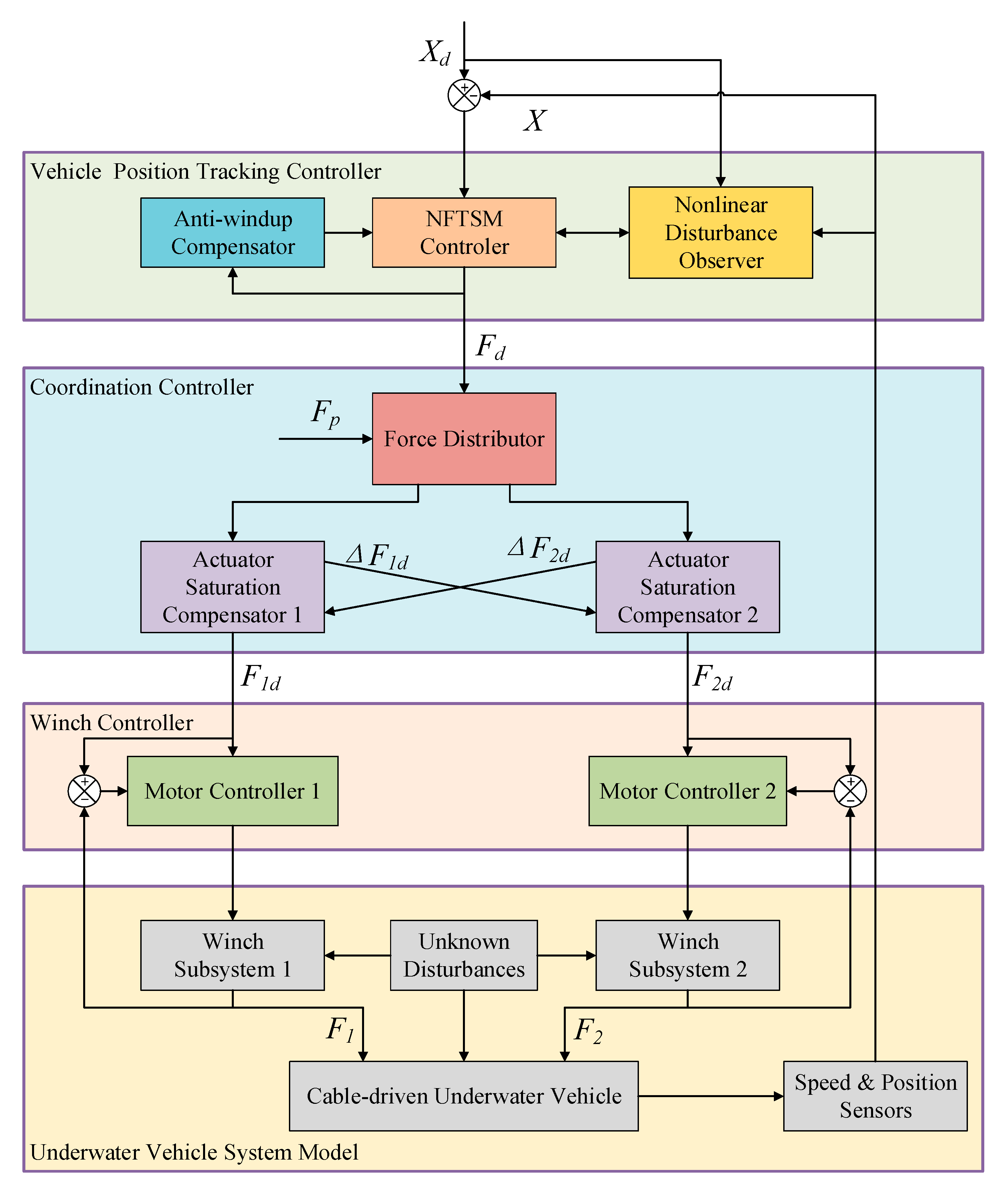
Based on the previously established model, the control problem can be formulated as follows:

Define: $x_1=x,\hspace{0.33em}{x}_2=\dot{x},\hspace{0.33em}{x}_3=F_1,\hspace{0.33em}{x}_4=F_2,\hspace{0.33em}{u}_1=F_d,\hspace{0.33em}{u}_2={\tau }_1,\hspace{0.33em}{u}_3={\tau }_2$.

The control model is represented as:

$$\left\{\begin{array}{l}{\dot{x}}_1=x_2\\ {\dot{x}}_2={\displaystyle \frac{F_d}{M}}-{\displaystyle \frac{F_f+F_w}{M}}+d_1\\ x_3={\displaystyle \frac{I_1}{R_1}}{\tau }_1-{\displaystyle \frac{{\dot{\varpi }}_1{J}_1}{R_1}}+d_2\\ x_4={\displaystyle \frac{I_2}{R_2}}{\tau }_2-{\displaystyle \frac{{\dot{\varpi }}_2{J}_2}{R_2}}+d_3\end{array}\right.$$

(12)

where $u_1$ represents the control input of the vehicle position tracking controller, $u_2$ represents the control input of winch controller 1, $u_3$ represents the control input of winch controller 2, $F_d=F_1-F_2$ is the total traction force of the vehicle, ${\varpi }_i={\dot{\theta }}_i$ is the angular velocity of the winch drum, and $d_1$, $d_2$, and $d_3$ are unknown but limited disturbances.

Simultaneously, the control input $u_i$, $i=1,\hspace{0.33em}2,\hspace{0.33em}3$ must satisfy the input saturation constraint $u_{i\min }<u_i<u_{i\max }$.

3. Control Design

The motion controller of the underwater vehicle comprises three primary components: dual-motor coordination controller, position tracking controller, and winch controller. Position and pre-tension commands are generated by the motion planner. The position tracking controller subsequently produces traction force commands based on these control instructions. The dual-motor coordination controller allocates the traction force commands to the two winch controllers, ultimately regulating the traction forces output by the winches.

The principle of control is shown in Figure 4.

3.1. Design of Vehicle-Position-Tracking Controller

The position tracking controller generates the total traction force command based on the position and pre-tension commands provided by the motion planner, making the vehicle converge to the target trajectory and propel it along the desired path.

The position tracking controller is structured around a nonsingular fast-terminal sliding-mode control (NFTSMC) framework. To maintain the robustness of sliding-mode control while mitigating the high-frequency chattering phenomenon, a saturation function replaces the traditional switching function. An auxiliary dynamic system is designed to compensate for actuator input saturation. Additionally, a fuzzy adaptive nonlinear disturbance observer (FANDO) is constructed to estimate and dynamically compensate for complex time-varying environmental disturbances.

3.1.1. Nonsingular Fast-Terminal Sliding-Mode Controller

A nonsingular fast-terminal sliding-mode controller (NFTSMC) was designed to address the unknown and complex disturbances experienced by underwater vehicle and its traction system during operation.

The system model of the vehicle is:

$$\left\{\begin{array}{l}{\dot{x}}_1=x_2\\ {\dot{x}}_2={\displaystyle \frac{u_1}{M}}-{\displaystyle \frac{F_f}{M}}-{\displaystyle \frac{F_w}{M}}+d_1\end{array}\right.$$

(13)

According to the saturation constraint that the winch needs to meet, $u_1$ also needs to meet the saturation constraint:

$$F_{\min }-F_{\max }\le u_1\le F_{\max }-F_{\min }$$

(14)

where $d_1$ is an unknown disturbance, satisfies $\left|d\right|\le D$ and $\left|\dot{d}\right|\le \Delta$.

Then, we define the tracking error as:

$$\left\{\begin{array}{l}{e}_1=x_1-x_{1d}\\ e_2={\dot{e}}_1=x_2-x_{2d}\end{array}\right.$$

(15)

We design a nonsingular fast-terminal sliding surface:

$$s=e_1+{\displaystyle \frac{1}{\beta }}{e_2}^{{\displaystyle \frac{p}{q}}}$$

(16)

where β > 0, p > q, p, and q are positive odd numbers, and p/q > 1.

Then, adopting exponential approach law and introducing saturation function to suppress chattering, we obtain

$$\dot{s}=-k\cdot \mathrm{sat}\left({\displaystyle \frac{s}{\varphi }}\right)-\eta s$$

(17)

where $\eta$ is the exponential convergence rate; $k>0$ is switching increase; $\varphi >0$ is the thickness of the boundary layer.

$$sat\left({\displaystyle \frac{s}{\varphi }}\right)=\left\{\begin{array}{l}\mathrm{sign}(s),\hspace{0.33em}\left|s\right|>\varphi \\ {\displaystyle \frac{s}{\varphi }}, \left|s\right|\le \varphi \end{array}\right.$$

(18)

The derivative of the sliding surface is:

$$\begin{array}{c}\dot{s}={\dot{e}}_1+{\displaystyle \frac{p}{q\beta }}{e}_2{{\displaystyle \frac{p}{q}}}^{-1}{\dot{e}}_2\\ \hspace{0.33em}\hspace{0.33em}\hspace{0.33em}\hspace{0.33em}\hspace{0.33em}\hspace{0.33em}\hspace{0.33em}\hspace{0.33em}\hspace{0.33em}\hspace{0.33em}\hspace{0.33em}\hspace{0.33em}\hspace{0.33em}\hspace{0.33em}\hspace{0.33em}\hspace{0.33em}\hspace{0.33em}\hspace{0.33em}\hspace{0.33em}\hspace{0.33em}\hspace{0.33em}\hspace{0.33em}\hspace{0.33em}\hspace{0.33em}=e_2+{\displaystyle \frac{p}{q\beta }}{e}_2{{\displaystyle \frac{p}{q}}}^{-1}\left({\displaystyle \frac{u_1}{M}}-{\displaystyle \frac{F_f+F_w}{M}}+d_1-{\dot{x}}_{2d}\right)\end{array}$$

(19)

Assuming the actuator is not saturated, the control input is decomposed into equivalent control $u_{eq}$ and switching control $u_{sw}$. Then,

$$u_1=u_{eq}+u_{sw}$$

(20)

Then, equivalent control requires offsetting nominal dynamics.

We let $d_1=0$ and $\dot{s}=0$; then,

$$0=e_2+{\displaystyle \frac{p}{q\beta }}{e_2}^{{\displaystyle \frac{p}{q}}-1}\left({\displaystyle \frac{u_1}{M}}-{\displaystyle \frac{F_f+F_w}{M}}-{\dot{x}}_{2d}\right)$$

(21)

The equivalent control law is obtained as follows:

$$u_{eq}=M\left({\dot{x}}_{2d}+{\displaystyle \frac{F_f+F_w}{M}}-\beta {\displaystyle \frac{q}{p}}{e}_2^{2-{\displaystyle \frac{p}{q}}}\right)$$

(22)

The switching control is used to compensate for disturbances and achieve convergence law:

$${\displaystyle \frac{p}{q\beta }}{e_2}^{{\displaystyle \frac{p}{q}}-1}\cdot {\displaystyle \frac{u_{sw}}{M}}=-\eta s-k\cdot \mathrm{sat}\left({\displaystyle \frac{s}{\varphi }}\right)-{\displaystyle \frac{p}{q\beta }}{e_2}^{{\displaystyle \frac{p}{q}}-1}{d}_1$$

(23)

The switching control law is obtained as:

$$u_{sw}=-M\left(\eta s+k\cdot \mathrm{sat}\left({\displaystyle \frac{s}{\varphi }}\right)\right)-M{d}_1$$

(24)

3.1.2. Saturation Compensation of the Actuators

We design an auxiliary dynamic system (ADS) to compensate for the saturation of the actuators.

Then, we define the saturation error as:

$$\Delta u_1=u_{1sat}-u_1\hspace{0.33em},\hspace{0.33em}\hspace{0.33em}{u}_{1sat}=sat(u_1)$$

(25)

The control input saturation function $sat(u_1)$ is represented as:

$$sat(u_1)=\left\{\begin{array}{l}{u}_{1\max }, u_1\ge u_{1\max }\\ u_1, u_{1\min }<u_1<u_{1\max }\\ u_{1\min }, u_1\le u_{1\min }\end{array}\right.$$

(26)

where $u_{1\max }$ is the maximum allowable traction force and $u_{1\min }$ is the minimum allowable traction force.

We introduce the auxiliary state $Z_a$ to compensate for the saturation effect. $Z_a$ can be expressed as:

$${\dot{Z}}_a=-k_a{Z}_a+\Delta u_1$$

(27)

where $k_a>0$.

Then, we modify the sliding surface and introduce auxiliary states to offset saturation errors:

$$s=e_1+{\displaystyle \frac{1}{\beta }}{\left(e_2+\gamma Z_a\right)}^{{\displaystyle \frac{p}{q}}},\hspace{0.33em}\hspace{0.33em}\hspace{0.33em}\hspace{0.33em}\gamma >0$$

(28)

The auxiliary compensation items can be represented as:

$$u_{aux}=-\gamma Z_a$$

(29)

where $\gamma$ is the compensation gain coefficient.

3.1.3. Fuzzy Adaptive Nonlinear Disturbance Observer

In practical control systems, external disturbances and model uncertainties are often key factors that affect control performance. Traditional sliding-mode control suppresses disturbances by designing high gain switching terms, but it strongly relies on the prior upper bound of disturbances, and excessive switching gains can lead to control input chattering, exacerbating actuator losses. To address this issue, the nonlinear disturbance observer (NDO) has been widely used to construct feedforward compensation mechanisms for disturbances.

To address the disturbance effects acting on the vehicle, a nonlinear disturbance observer (NDO) is designed as follows:

$$\dot{\widehat{d}}=L_1\left({\dot{e}}_2-{\displaystyle \frac{\mathrm{sat}\left(u_1\right)}{M}}+{\displaystyle \frac{F_f+F_w}{M}}+{\dot{x}}_{2d}\right)-L_1\widehat{d}$$

(30)

where L₁ is the observer gain,

The estimation error of the observer is represented as:

$${\tilde{d}}_1=d_1-{\widehat{d}}_1, \left|{\tilde{d}}_1\right|\le {\delta }_1$$

(31)

where δ₁ is the upper limit of error.

The disturbance compensation term in the controller can be represented as:

$$u_{NDO}=-M\widehat{d}$$

(32)

In practical scenarios, the range of disturbances acting on the vehicle varies with its motion speed. In the design of a nonlinear disturbance observer (NDO), parameter selection directly impacts the estimation accuracy and robustness against unknown disturbances. Although conventional NDO methods ensure the stability of estimation errors by predefining disturbance bounds, fixed-parameter designs often struggle to achieve an optimal trade-off between rapid response and overshoot suppression when facing dynamic variations in disturbance amplitude, frequency, and other ranges. This challenge becomes particularly evident when disturbances exhibit time-varying characteristics or multi-source coupling, where fixed-gain observers tend to increase conservatism or degrade dynamic performance. To address these limitations, this paper introduces a fuzzy-logic-based adaptive parameter adjustment mechanism that dynamically tunes key NDO parameters to adapt to changing disturbance characteristics.

Define the fuzzy input variables as disturbance estimation error ${\tilde{d}}_1$ and its rate of change ${\dot{\tilde{d}}}_1$, gain adjustment amount is $\Delta L_1$. The time-varying gain can be represented as:

$$L_1(t)=L_0+\Delta L_1\left(t\right), L_0>0$$

(33)

The adaptive law is represented as:

$$\Delta L_1\left(t\right)=K_f\cdot \mathrm{FLS}(\tilde{d}, \dot{\tilde{d}}), K_f>0$$

(34)

where K_f is the fuzzy output gain.

3.1.4. Total Control Law of the Position Tracking Controller

Considering all components, the total resulting control law can be written in the form of:

$$u=u_{eq}+u_{sw}+u_{aux}+u_{NDO}$$

(35)

That is,

$$u_1=M\left({\dot{x}}_{2d}+{\displaystyle \frac{F_f+F_w}{M}}-\beta {\displaystyle \frac{q}{p}}{e}_2^{2-{\displaystyle \frac{p}{q}}}\right)-M\left(\eta s+k\cdot \mathrm{sat}\left({\displaystyle \frac{s}{\varphi }}\right)\right)-\gamma Z_a-M\widehat{d}$$

(36)

3.1.5. Proof of Stability

Step 1: Construction of a Lyapunov function.

Construction a Lyapunov function as follows, including sliding surface, auxiliary dynamic system, disturbance estimation error, and gain adaptive error.

$$V={\displaystyle \frac{1}{2}}{s}^2+{\displaystyle \frac{1}{2}}{Z}_a^2+{\displaystyle \frac{M}{2L\left(t\right)}}{\tilde{d}}_1^2+{\displaystyle \frac{1}{2K_f}}\Delta L{\left(t\right)}^2$$

(37)

Step 2: Derivative analysis.

The derivative of sliding-mode surface is:

$${\dot{V}}_s=s\dot{s}=-\eta s^2-ks\cdot \mathrm{sat}\left({\displaystyle \frac{s}{\varphi }}\right)+{\displaystyle \frac{p}{q\beta M}}s{\left(e_2+\gamma Z_a\right)}^{{\displaystyle \frac{p}{q}}-1}{\tilde{d}}_1$$

(38)

The derivative of auxiliary dynamic system is:

$${\dot{V}}_z=Z_a{\dot{Z}}_a=-k_a{Z}_a^2+Z_a\Delta F_d$$

(39)

The derivative of disturbance estimation error is:

$${\dot{V}}_{{\tilde{d}}_1}={\displaystyle \frac{M}{L\left(t\right)}}{\tilde{d}}_1{\dot{\tilde{d}}}_1={\displaystyle \frac{M}{L\left(t\right)}}{\tilde{d}}_1\left({\dot{d}}_1-L\left(t\right){\tilde{d}}_1-\Delta L\left(t\right)\cdot \mathrm{Residual} \mathrm{Error}\right)$$

(40)

The derivative of gain adaptive is:

$${\dot{V}}_{\Delta L}={\displaystyle \frac{1}{K_f}}\Delta L\left(t\right)\Delta \dot{L}\left(t\right)=\Delta L\left(t\right)\cdot \mathrm{FLS}({\tilde{d}}_1,\hspace{0.33em}{\dot{\tilde{d}}}_1)$$

(41)

According to the design of fuzzy rules, it can be concluded that:

$${\dot{V}}_{\Delta L}\le -\mu \Delta L{\left(t\right)}^2$$

(42)

We select parameters that meet the following requirements:

Switching gain: $k\ge {\displaystyle \frac{2pD}{q\beta M}}{‖{\left(e_2+\gamma Z_a\right)}^{{\displaystyle \frac{p}{q}}-1}‖}_{\max }+\eta$;

Observer gain: $L\left(t\right)\ge \Delta$;

Auxiliary Dynamic System gain: ${\alpha }_a>0$, $\gamma \ge {\displaystyle \frac{2F_{\max }}{k_a}}$.

Thus, we obtain:

$$\dot{V}\le -\eta s^2-k_a{Z}_a^2-{\displaystyle \frac{M}{2}}{\tilde{d}}_1^2-\mu \Delta L{\left(t\right)}^2\le 0$$

(43)

Then, the system is globally asymptotically stable.

3.2. Design of Dual-Motor Coordination Controller

The dual-motor differential tension coordination controller distributes traction commands to the two winch controllers based on the driving force command $F_d$ provided by the motion controller, and the set preload force command $F_p$, combined with the actuator saturation compensator.

To maintain tension between the two wire ropes during movement, the minimum traction force commands for the winch are $F_{1\min }>0$ and $F_{2\min }>0$.

The winch also has maximum traction forces, which are $F_{1\max }$ and $F_{2\max }$.

$F_p$ is the system preload force. It is used to maintain tension in the traction system. To ensure that the tension does not exceed the output limit of the winch, $F_p$ should meet the following requirements:

$$2\times \max \left(F_{1\min },\hspace{0.33em}{F}_{2\min }\right)<F_p<2\times \min \left(F_{1\max },\hspace{0.33em}{F}_{2\max }\right)$$

(44)

As F_d changes, F_1d or F_2d will be less than their minimum value or greater than their maximum value, indicating saturation of the actuator. To address this issue, an actuator saturation compensator is introduced.

For winch 1, the saturation error of its output traction force can be expressed as:

$$\Delta F_{1d}=F_{1sat}-F_{1d}$$

(45)

where $F_{1d}$ is the expected traction force of winch 1 output by the motion controller and $F_{1sat}$ is the traction force output by winch 1 after saturation limitation, which can be expressed as:

$$F_{1sat}=\left\{\begin{array}{l}{F}_{1\max }, F_{1d}>F_{1\max }\\ F_{1d}, F_{1\min }\le F_{1d}\le F_{1\max }\\ F_{1\min }, F_{1d}<F_{1\min }\end{array}\right.$$

(46)

Similarly, the saturation error of winch 2 output traction force can be expressed as

$$\Delta F_{2d}=F_{2sat}-F_{2d}$$

(47)

where $F_{2d}$ is the expected traction force of winch 2 output by the motion controller, $F_{2sat}$ is the traction force output by winch 2 after saturation limitation, which can be expressed as:

$$F_{2sat}=\left\{\begin{array}{l}{F}_{2\max }, F_{2d}>F_{1\max }\\ F_{2d}, F_{2\min }\le F_{2d}\le F_{2\max }\\ F_{2\min }, F_{2d}<F_{2\min }\end{array}\right.$$

(48)

When winch 1 is saturated, we limit the traction command to winch 1 and adjust the traction command to winch 2 so that the total traction force applied to the vehicle is not affected. Similarly, when winch 2 is saturated, we limit the traction command to winch 2 and adjust the traction command to winch 1.

The traction force command of winch 1 is represented as:

$$F_{1d}={\displaystyle \frac{1}{2}}(F_p+F_d)+\Delta F_{2d}$$

(49)

The traction force command of winch 2 is represented as:

$$F_{2d}={\displaystyle \frac{1}{2}}(F_p-F_d)+\Delta F_{1d}$$

(50)

3.3. Design of Winch Controller

Based on the winch model, we define:

$$x_3=F_1,\hspace{0.33em}{x}_4=F_2,\hspace{0.33em}{u}_2={\tau }_1,\hspace{0.33em}{u}_3={\tau }_2$$

(51)

For winch 1, the dynamic model can be described as:

$$x_3={\displaystyle \frac{I_1}{R_1}}{u}_2-{\displaystyle \frac{{\dot{\varpi }}_1{J}_1}{R_1}}+d_2$$

(52)

where ${\varpi }_1$ represents the rotational speed of the winch, measured by a rotational speed sensor.

The feedforward compensation term is derived from the dynamic model as:

$$u_{2ff}={\displaystyle \frac{R_1}{I_1}}\left(x_{3d}+{\displaystyle \frac{{\dot{\varpi }}_1{J}_1}{R_1}}\right)$$

(53)

To address model uncertainties and disturbance, a PID controller is introduced as:

$$u_{2fb}=K_{p1}{e}_3+K_{i1}{\displaystyle {\int }_0^t{e}_3\left(\xi \right)d\xi }+K_{d1}{\displaystyle \frac{d{e}_3}{dt}}, e=x_3-x_{3d}$$

(54)

The resulting control law can be represented as:

$$u_2=u_{2ff}+u_{2fb}$$

(55)

Similarly, for winch 2, the dynamic model is described as:

$$x_4={\displaystyle \frac{I_2}{R_2}}{u}_3-{\displaystyle \frac{{\dot{\varpi }}_2{J}_2}{R_2}}+d_3$$

(56)

where ${\varpi }_2$ represents the rotational speed of the winch.

The feedforward compensation term is derived from the dynamic model as:

$$u_{3ff}={\displaystyle \frac{R}{I}}\left(x_{4d}+{\displaystyle \frac{\alpha J}{R}}\right)$$

(57)

To address model uncertainties and disturbance, a PID controller is introduced as:

$$u_{3fb}=K_{p2}{e}_4+K_{i2}{\displaystyle {\int }_0^t{e}_4\left(\xi \right)d\xi }+K_{d2}{\displaystyle \frac{d{e}_4}{dt}}, e=x_4-x_{4d}$$

(58)

The resulting control law can be represented as:

$$u_3=u_{3ff}+u_{3fb}$$

(59)

4. Simulation Results

In this section, simulations are conducted on the trajectory-tracking control of a flexible-towed underwater vehicle to validate the performance of the proposed controller.

4.1. Simulation Preparation

The parameters of the simulation model are listed in

Table 1. Simulation model parameters.

Parameter	Definition	Value	Unit
M	Mass of the vehicle	$1\hspace{0.33em}\times \hspace{0.33em}{10}^4$	kg
$C_d$	Vehicle drag coefficient	0.3	$\mathrm{N}\hspace{0.33em}\times \hspace{0.33em}{\mathrm{s}}^2/\hspace{0.33em}{\mathrm{m}}^2$
D	Diameter of the vehicle	2	m
H	Height of the underwater vehicle	3	m
$\rho$	Water density	1000	$\mathrm{kg}\hspace{0.33em}\cdot \hspace{0.33em}{\mathrm{m}}^3$
${\overline{F}}_N$	Average pressure exerted by the vehicle on the track	$4.9 \times {10}^3$	N
$L_0$	Total length of the track.	50	m
J	Moment of inertia of the winch	1.8	$\mathrm{kg}\hspace{0.33em}\cdot \hspace{0.33em}{\mathrm{m}}^2$
R	Radius of the winch drum	0.8	m
I	Gear reduction ratio of the winch	36	/
$F_{\max }$	Upper force limit of the winch	$6\hspace{0.33em}\times \hspace{0.33em}{10}^3$	N
$F_{\min }$	Lower force limit of the winch	$200$	N
A	Cross-sectional area of the steel wire rope	$4.52\hspace{0.33em}\times \hspace{0.33em}{10}^{-4}$	${\mathrm{m}}^2$
E	Equivalent axial elastic modulus of the steel wire rope	80	GPa
c	Equivalent damping coefficient of the steel wire rope	1000	$\mathrm{N}\hspace{0.33em}\times \hspace{0.33em}\mathrm{s}\hspace{0.33em}/\hspace{0.33em}\mathrm{m}$

.

In this paper, we conducted simulation studies under both disturbance-free conditions and scenarios with nonlinear time-varying disturbances. For the disturbance-free case, control performance comparisons are performed between the proposed controller and a PID cascade controller. Under disturbed conditions, the proposed controller is comparatively analyzed against two approaches: (1) PID cascade control and (2) nonsingular fast-terminal sliding-mode control (NFTSMC) without an observer. The control methods participating in the comparative study are summarized in

Table 2. Control methods utilized in the simulation.

Method	Description
FANDO-NFTSM	Proposed control
NFTSM	Nonsingular fast-terminal sliding-mode control without an observer
PID	PID cascade control

.

The parameters of NFTSM are selected as p = 5, q = 3, beta = 0.05, eta = 0.05, k = 0.5, and phi = 0.5. The parameters of PID cascade control are selected as kp1 = 10, ki1 = 0.1, kp2 = 2, and ki2 = 0.05.

Perform constant speed tracking and trajectory tracking under simulated experimental conditions separately with and without disturbance. The preload $F_p$ is set at 2000 Newtons.

In uniform-speed tracking, the underwater vehicle tracking along a reference trajectory, which is defined as:

$$x_d\left(t\right)=1.5t, t\le 25$$

(60)

Due to the maximum operating range, the simulation duration was set to 25 s.

In the experimental conditions, the reference trajectory consists of three different stages, (a) uniformly accelerated motion, (b) uniform motion, and (c) uniformly decelerated motion, as shown below,

$$x_d\left(t\right)=\left\{\begin{array}{l}0.05t^2,\hspace{0.33em}\hspace{0.33em}\hspace{0.33em}\hspace{0.33em}\hspace{0.33em}\hspace{0.33em}\hspace{0.33em}\hspace{0.33em}\hspace{0.33em}\hspace{0.33em}\hspace{0.33em}\hspace{0.33em}\hspace{0.33em}\hspace{0.33em}\hspace{0.33em}\hspace{0.33em}\hspace{0.33em}\hspace{0.33em}\hspace{0.33em}\hspace{0.33em}\hspace{0.33em}\hspace{0.33em}\hspace{0.33em}t\le 18\\ 1.8t+9,\hspace{0.33em}\hspace{0.33em}\hspace{0.33em}\hspace{0.33em}\hspace{0.33em}\hspace{0.33em}\hspace{0.33em}\hspace{0.33em}\hspace{0.33em}\hspace{0.33em}\hspace{0.33em}\hspace{0.33em}\hspace{0.33em}\hspace{0.33em}\hspace{0.33em}\hspace{0.33em}\hspace{0.33em}\hspace{0.33em}\hspace{0.33em}\hspace{0.33em}\hspace{0.33em}18<t\le 29\\ -0.075t^2+6.15t-79.275,\hspace{0.33em}\hspace{0.33em}\hspace{0.33em}\hspace{0.33em}\hspace{0.33em}\hspace{0.33em}29<t\le 41\\ 46.8,\hspace{0.33em}\hspace{0.33em}\hspace{0.33em}\hspace{0.33em}\hspace{0.33em}\hspace{0.33em}\hspace{0.33em}\hspace{0.33em}\hspace{0.33em}\hspace{0.33em}\hspace{0.33em}\hspace{0.33em}\hspace{0.33em}\hspace{0.33em}\hspace{0.33em}\hspace{0.33em}\hspace{0.33em}\hspace{0.33em}\hspace{0.33em}\hspace{0.33em}\hspace{0.33em}\hspace{0.33em}\hspace{0.33em}\hspace{0.33em}t>41\end{array}\right.$$

(61)

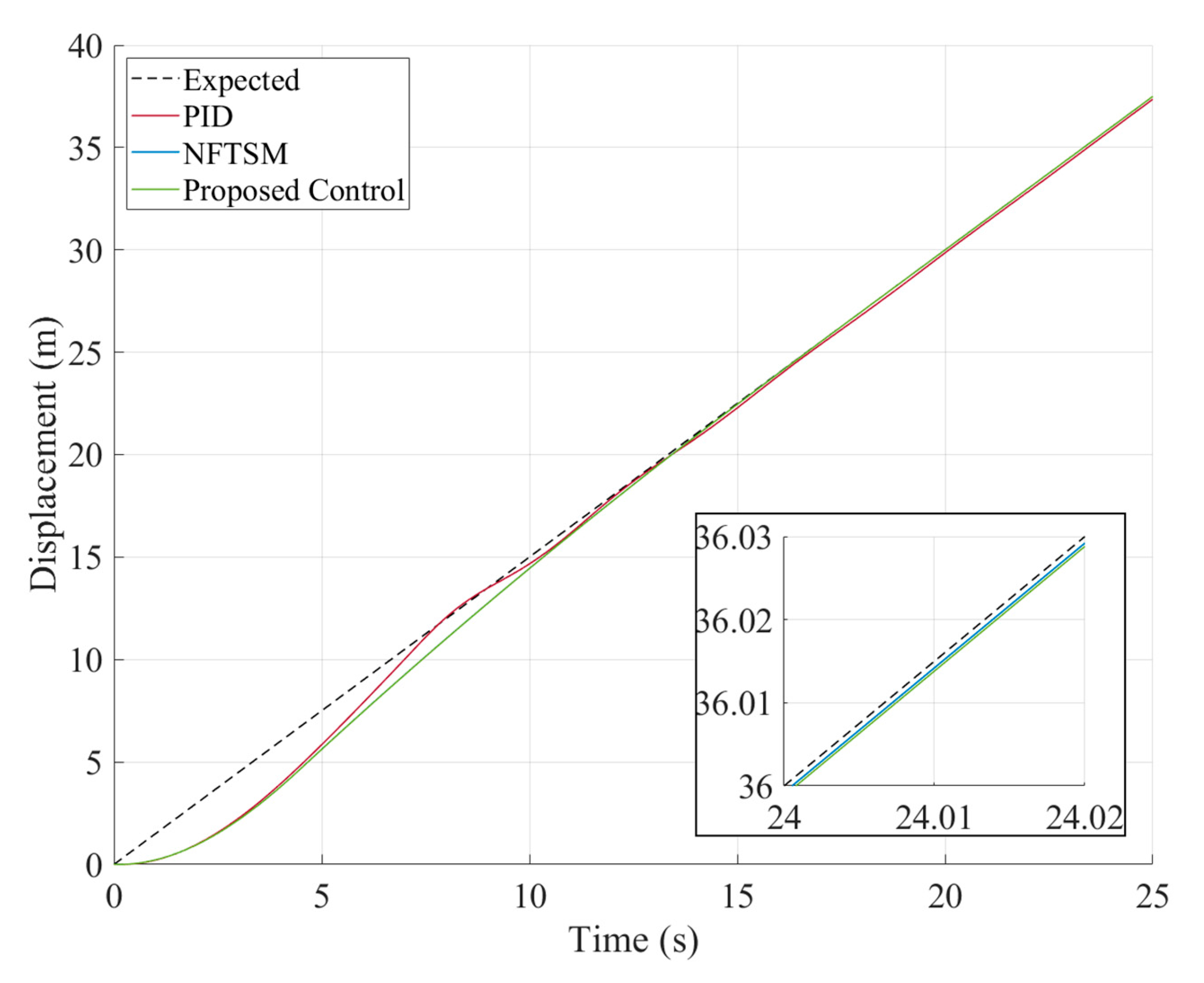
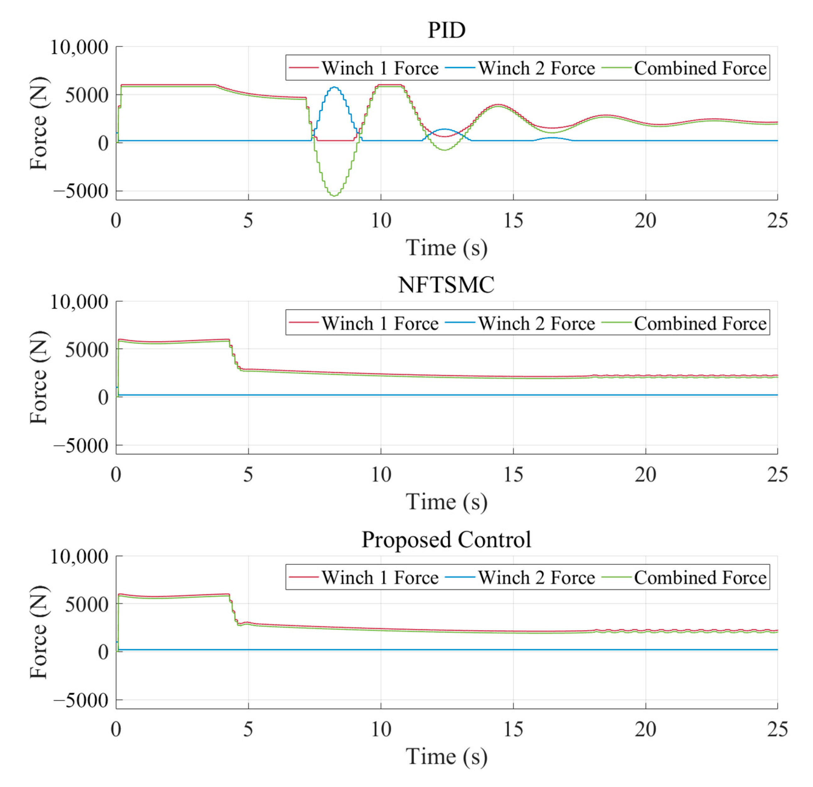
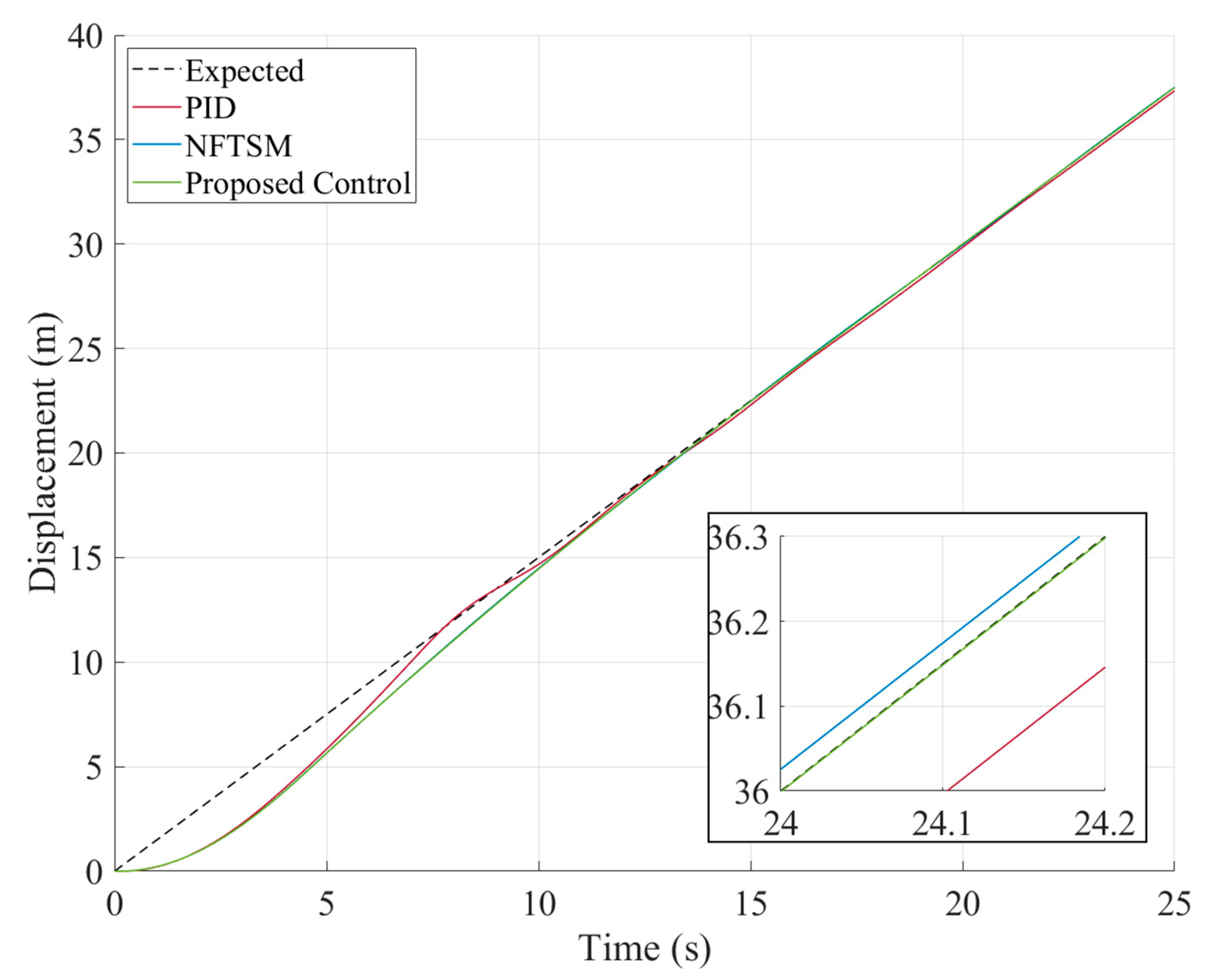
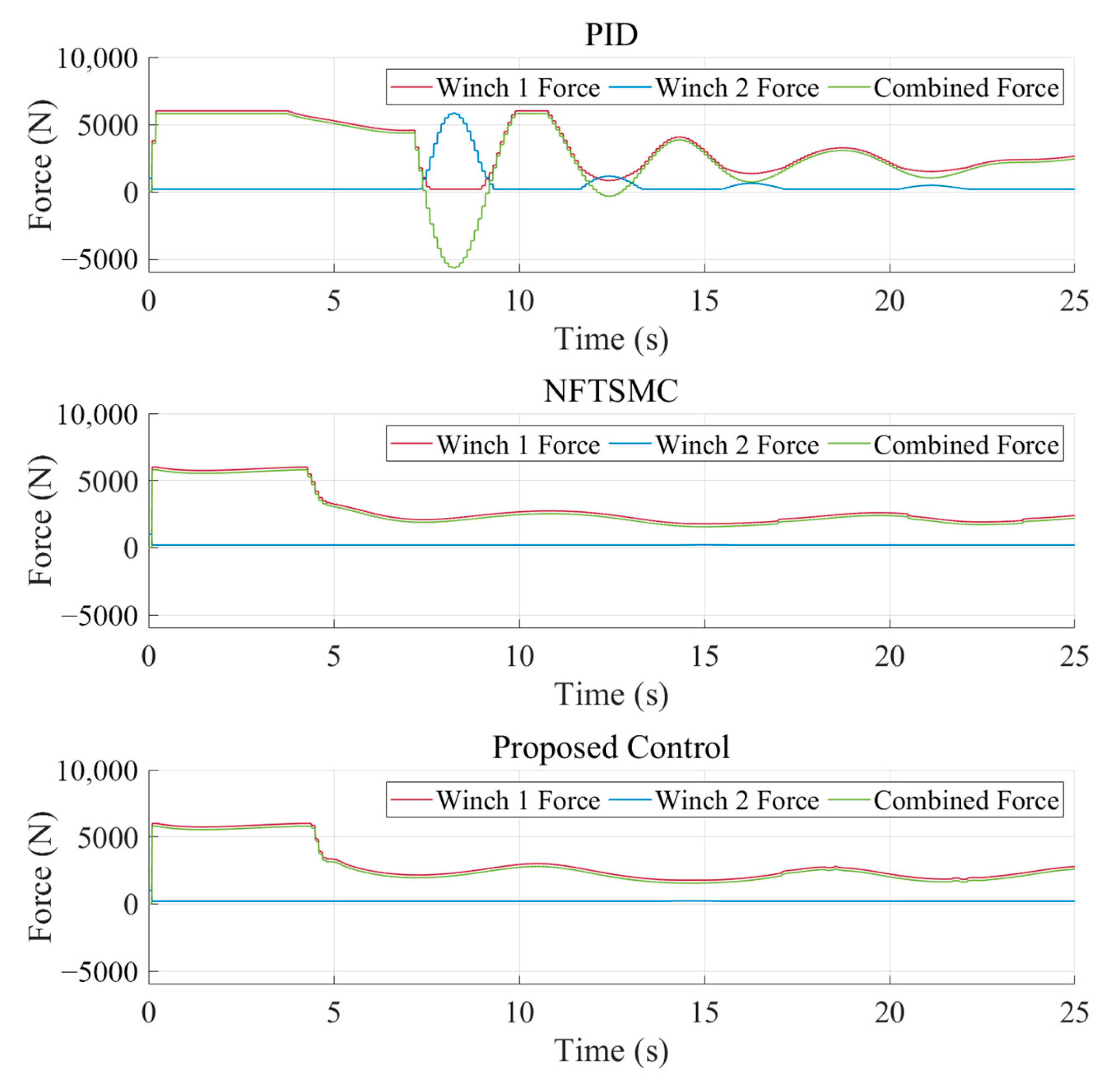
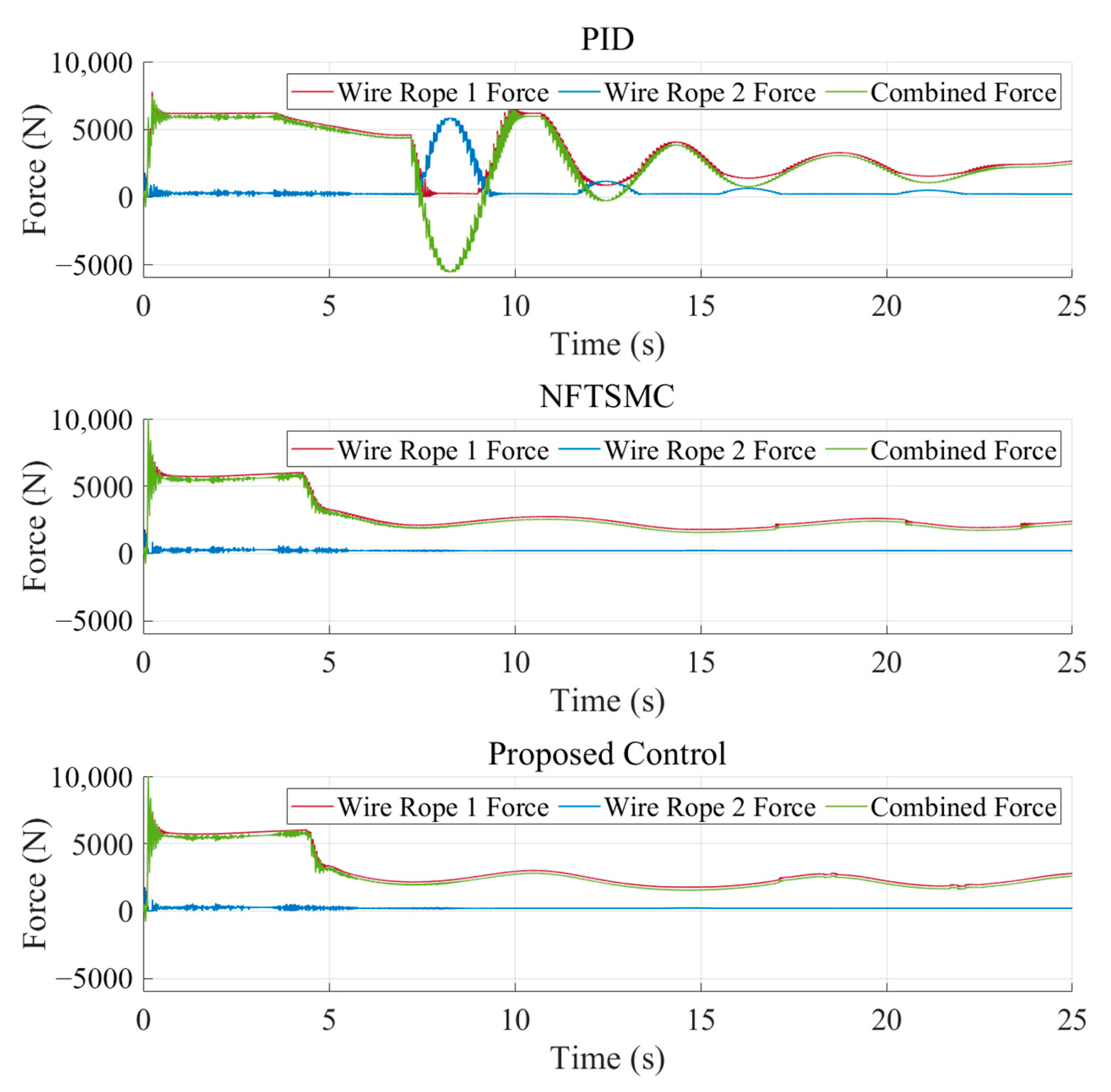
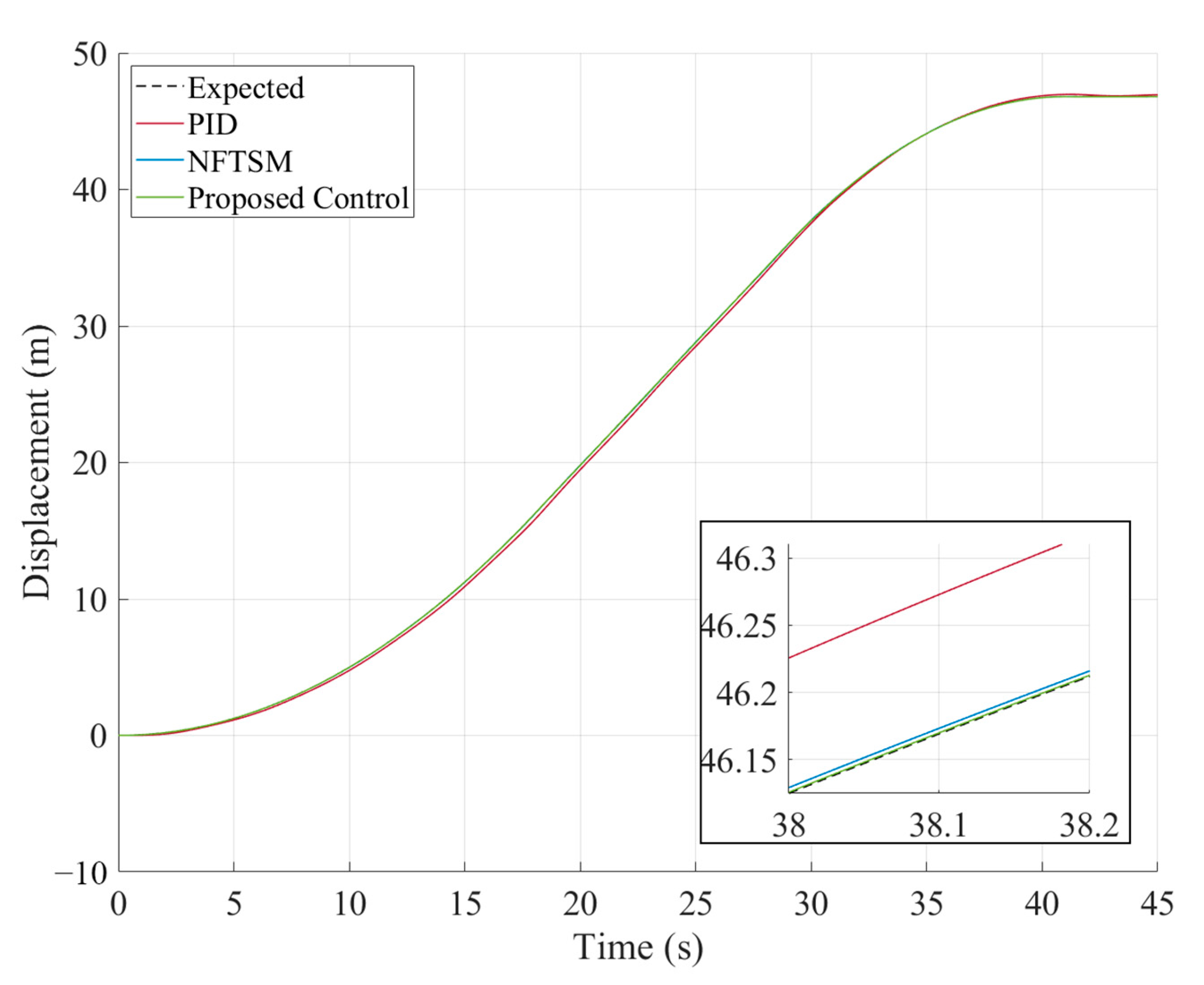
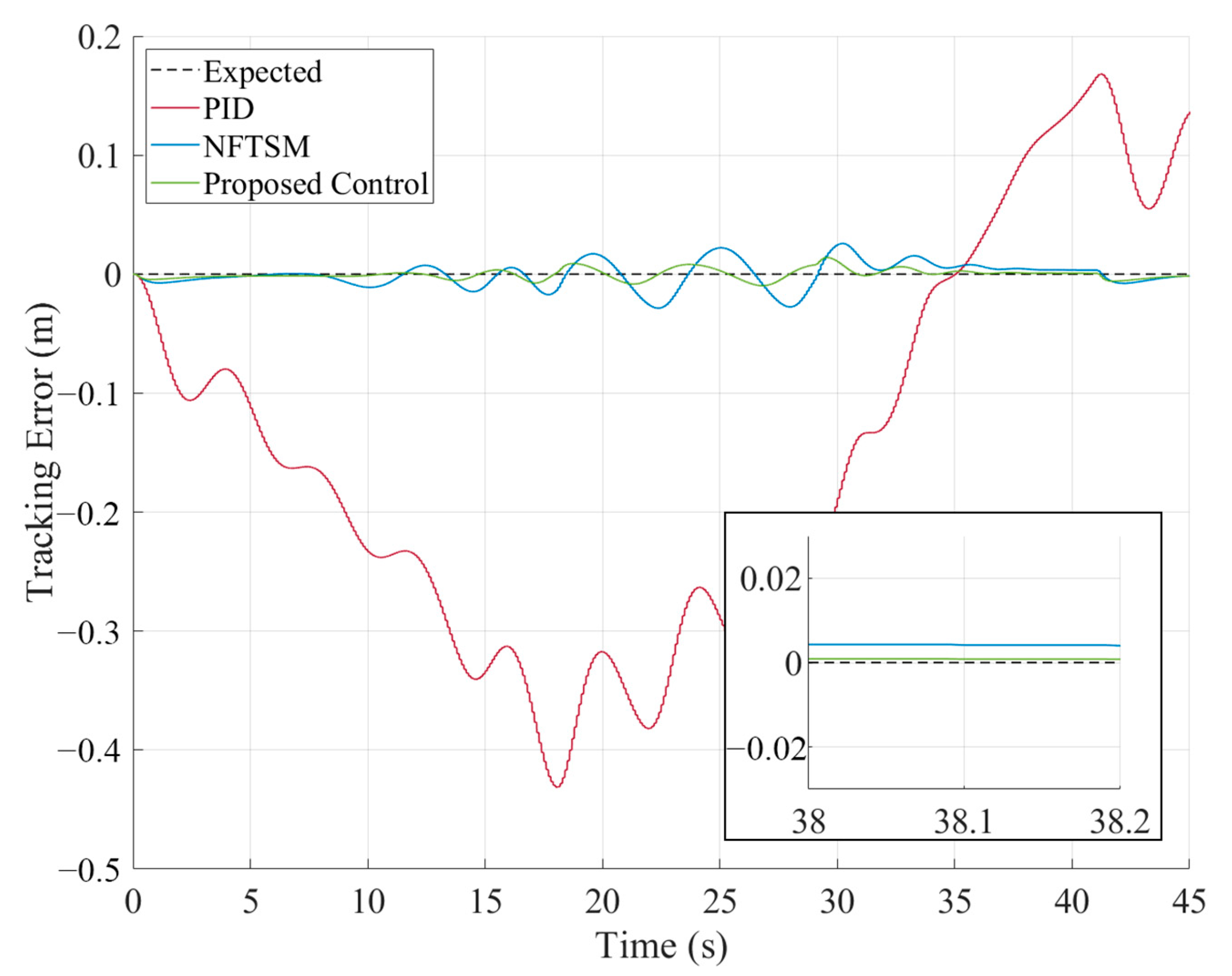
4.2. Trajectory Tracking Without Disturbances

Case1: Uniform-speed tracking without disturbances.

The tracking results are shown in Figure 5, Figure 6, Figure 7 and Figure 8.

It can be observed that both methods are able to converge the vehicle to the desired trajectory. However, the PID cascade control exhibits significantly slower response in transient adjustments. Furthermore, as shown in Figure 6, the proposed controller achieved faster convergence rates and smaller steady-state errors compared to the PID cascade control.

Case 2: Trajectory tracking under simulated experimental conditions without disturbances.

The tracking results are presented in Figure 9, Figure 10, Figure 11 and Figure 12.

The results demonstrate that both methods are capable of realizing the desired control objectives. The convergence time and steady-state error of the proposed controller is significantly smaller than the PID cascade controller. From the comparison between Figure 7 and Figure 10, compared to constant speed tracking, the simulated experimental condition has a longer acceleration stage, which causes the tension on the steel wire rope to slowly increase, significantly reducing the shaking of the wire rope tension. This indicates that reasonable trajectory planning can significantly improve the smoothness of the motion process.

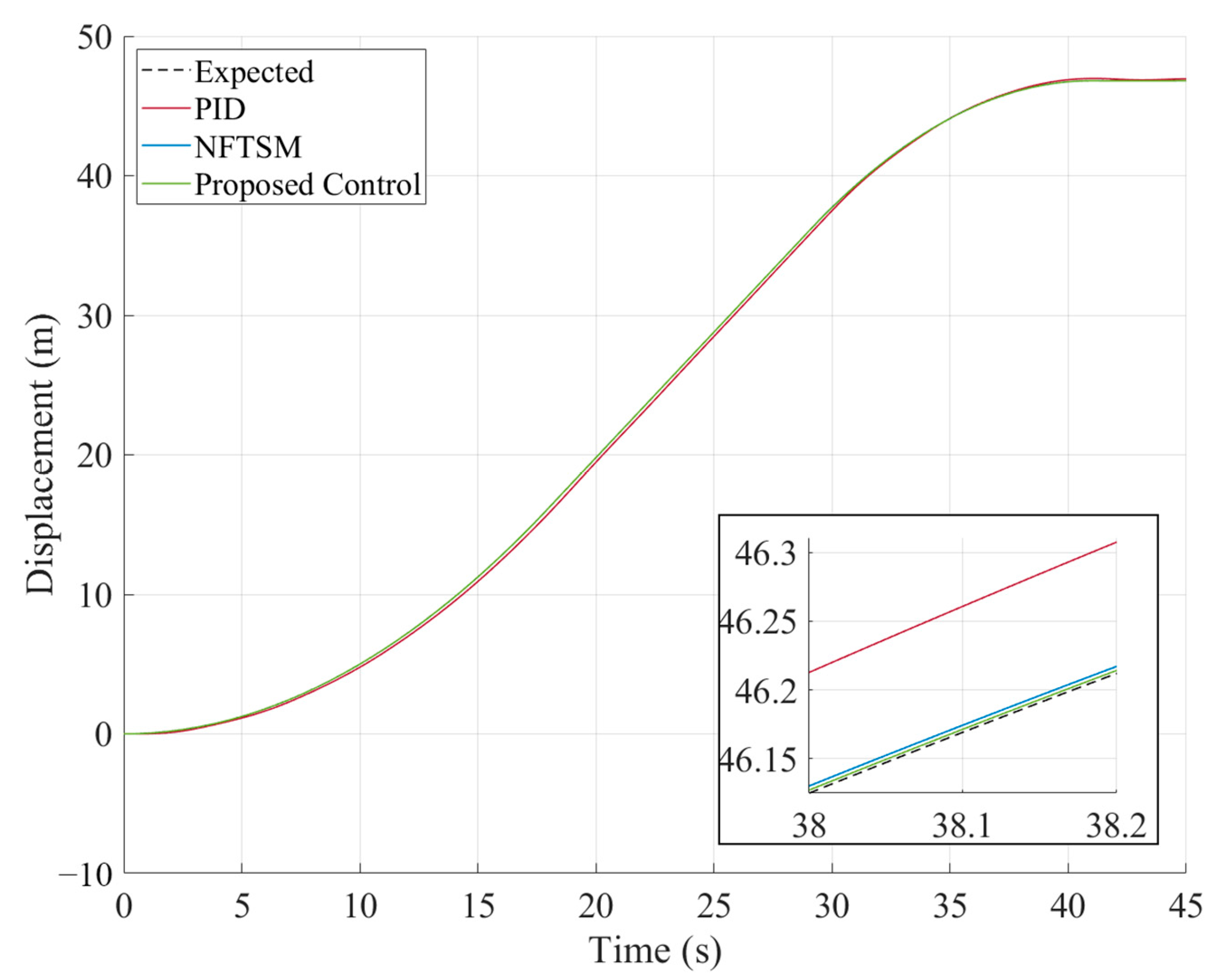
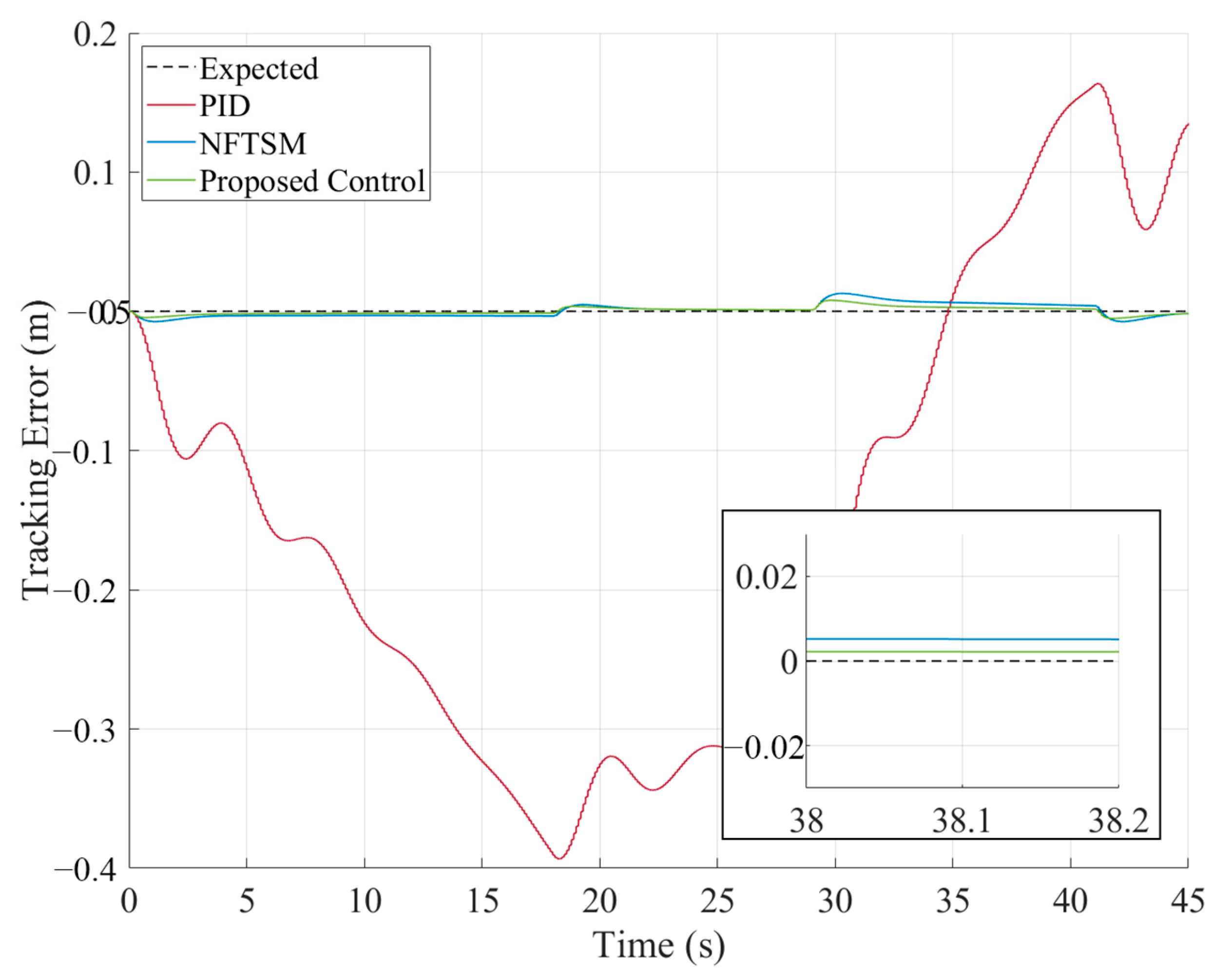
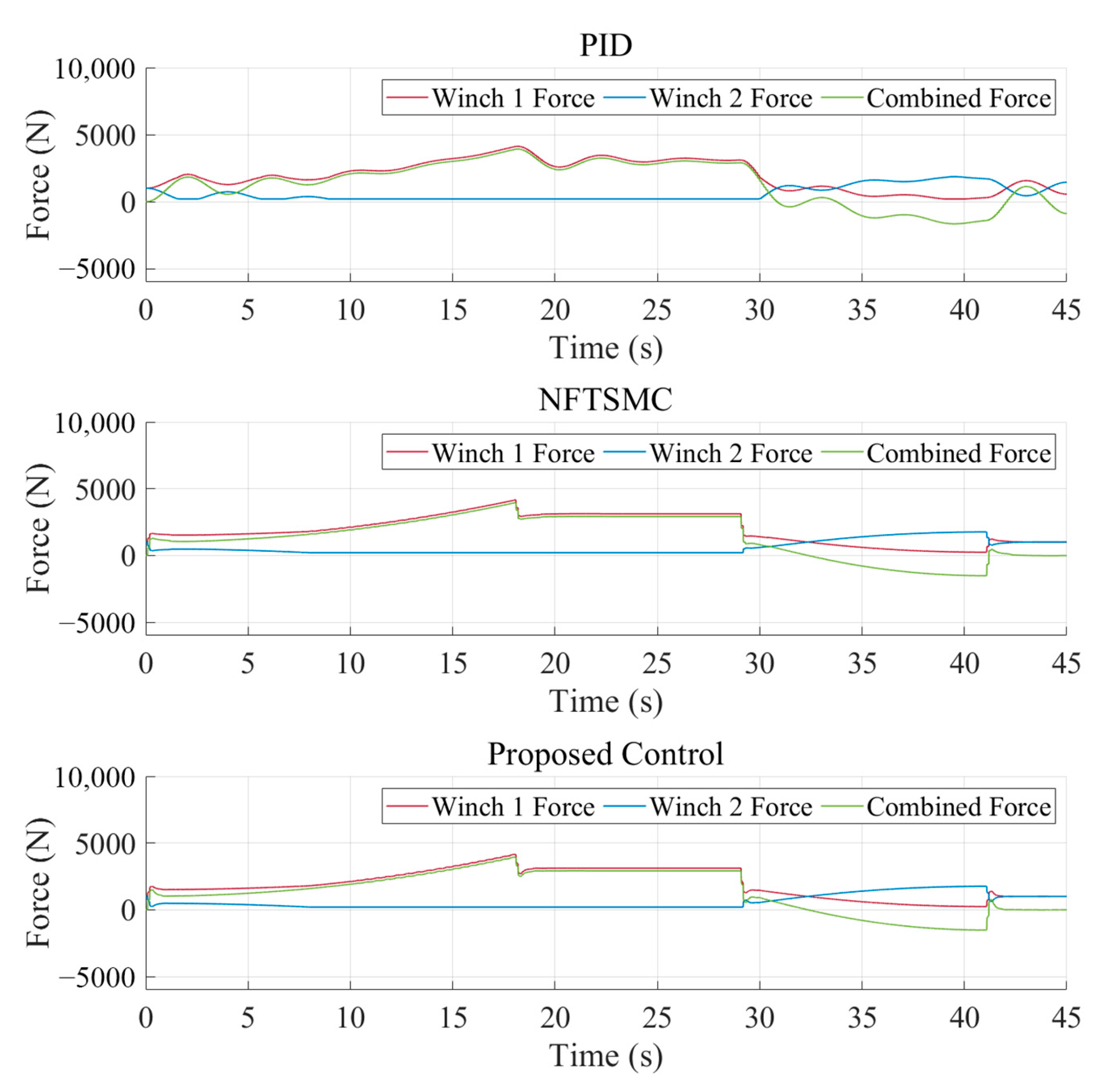
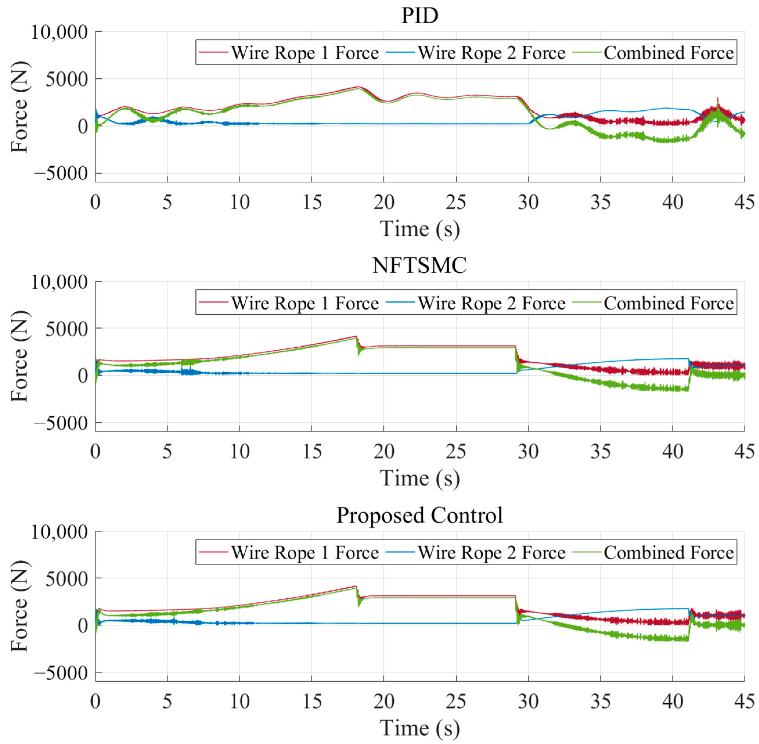
4.3. Trajectory Tracking Under Complex Time-Varying Disturbances

Underwater vehicles are subjected to complex time-varying disturbances from multiple sources during submerged operations. A representative example is the periodic variation in drag force caused by fluctuations in the pressure distribution over the vehicle’s surface, which results from periodically shedding vortices. The amplitude of this disturbance can be approximated as:

$$\Delta F_w\approx 0.1~0.3F_w$$

(62)

The frequency is governed by the Strouhal number relation as:

$$f=St\cdot {\displaystyle \frac{U}{D}}$$

(63)

where St is the Strouhal number (dimensionless); f is the vortex shedding frequency (Hz); D is the characteristic length of the vehicle (diameter for cylinder) (m); U is the free-stream flow velocity (m/s).

To account for this characteristic, periodic time-varying disturbances are introduced into the simulation model. The disturbance can be represented as:

$$d_1\left(t\right)={\displaystyle \frac{\Delta F_w(t)\sin \left(2\pi \frac{St\cdot U}{D}\cdot t\right)}{M}}$$

(64)

The set parameters are $\Delta F_w=0.2F_w$, $St=0.2$, $D=2$. The free-stream velocity equals the vehicle’s velocity, that is $U={\dot{x}}_1$.

Case 3: Uniform-speed tracking under complex time-varying disturbances.

The tracking results are shown in Figure 13, Figure 14, Figure 15 and Figure 16.

It can be observed that, after introducing time-varying disturbances, all three methods enable the vehicle to follow the target trajectory during uniform-speed tracking. As shown in Figure 14, when the FANDO is utilized for feedforward disturbance compensation, the overshoot, convergence rate, and steady-state tracking error are significantly smaller compared to the case without the observer.

Case 4: Trajectory tracking under simulated experimental conditions under complex time-varying disturbances.

The tracking results are shown in Figure 17, Figure 18, Figure 19 and Figure 20.

As shown in Figure 17 and Figure 18, compared to the disturbance-free case, the time-varying disturbances indeed degrade the steady-state tracking performance of the vehicle. Figure 18 further reveals that, when the FANDO provides feedforward compensation for disturbances, the steady-state tracking error of the vehicle is significantly smaller than that without the observer.

To further illustrate the differences in tracking performance between the NFTSM and the proposed control methods, a data comparison between the two approaches during the steady-state phase is provided. Among the three metrics analyzed, the mean absolute value (MAE) of the tracking error reflects control accuracy, the maximum absolute value of the tracking error indicates the worst-case deviation; the mean squared error (MSE) of the tracking error quantifies stability and fluctuation range.

The results clearly demonstrate from Figure 21 that, for the proposed controller, compared to the baseline NFTSM without the disturbance observer, the absolute mean value of the tracking error decreased by 76%, the absolute maximum value of the tracking error decreased by 67%, and the mean square error decreased by 93.5%.

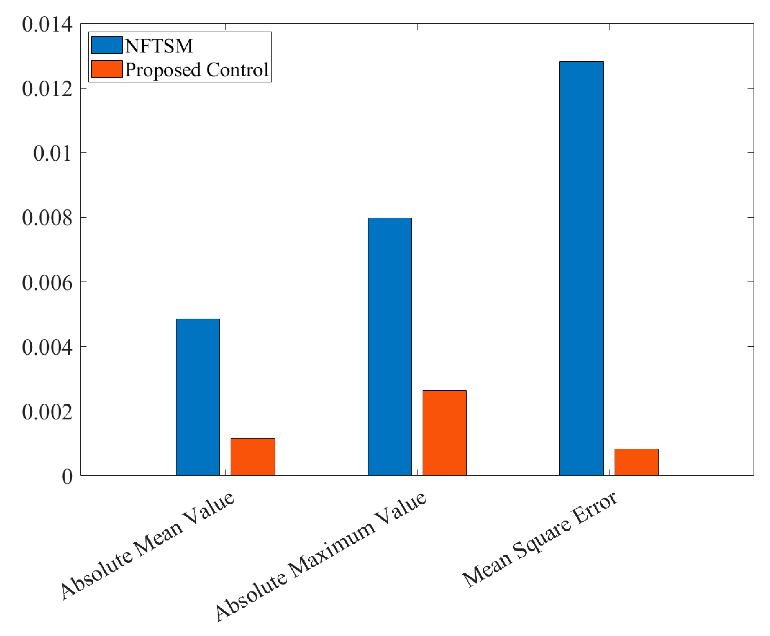
4.4. Discussion of Simulation Results

Based on the simulation results, it can be clearly demonstrated that the proposed controller achieves precise and robust trajectory tracking despite the nonlinear wire rope dynamics, multiple sources of unknown uncertainties, and input saturation. Furthermore, the proposed controller exhibits superior tracking accuracy and stability compared to the other two control algorithms. Therefore, the proposed controller is proven to be effective and suitable for the motion control of flexible-towed underwater vehicles.

5. Conclusions

This paper proposes a novel model for an underwater vehicle based on dual-motor-coordinated flexible towing. First, nonlinear wire rope dynamics, vehicle kinematic, and winch dynamic models are established. Subsequently, a dual-motor differential tension coordination controller is designed. Furthermore, a nonsingular fast-terminal sliding-mode control controller is developed, integrating a fuzzy adaptive nonlinear disturbance observer (FANDO) and an input-saturation-compensated auxiliary dynamic system. The main contributions of this paper can be summarized as follows:

(1)

A coupled dynamic model incorporating the underwater vehicle, winches, and steel wire ropes were established. This model explicitly accounts for the nonlinear hydrodynamic disturbances acting on the underwater vehicle and the nonlinear dynamic characteristics of the wire ropes.

(2)

A differential tension coordinated control strategy for dual winches was proposed. This strategy dynamically regulates the outputs of dual winches to ensure the precise generation of the driving forces required for vehicle motion while simultaneously avoiding tension chattering in the wire ropes and actuator saturation.

(3)

A nonsingular fast-terminal sliding-mode control method integrated with a fuzzy adaptive nonlinear state observer and an input-saturation-compensated auxiliary dynamic system was implemented. This approach enables the underwater vehicle to achieve rapid convergence to reference trajectories and maintain accurate trajectory tracking under nonlinear time-varying disturbances.

Theoretically, the proposed control method can be applied to any bounded unknown uncertainties, as its design does not require prior knowledge of uncertainties. By relaxing the requirement for prior knowledge of uncertainty bounds, the method enhances disturbance rejection capabilities.

However, the following issues must be addressed before practical implementation: we must simplify the control algorithm or introduce parameter-optimization mechanisms to improve control performance; we must optimize the towing system’s tension based on real-world conditions to reduce continuous operational loads on electric winches.

This work represents an early stage of research in the design of dual-motor-coordinated flexible towing systems for underwater vehicles. The challenges will be resolved in future studies.

References

1. You, S.S.; Lim, T.W.; Kim, J.Y.; Choi, H.S. Dynamics and Robust Control of Underwater Vehicles for Depth Trajectory Following. Proc. Inst. Mech. Eng. 2013, 227, 107–113. [Google Scholar] [CrossRef]
2. Koren, Y. Cross-Coupled Biaxial Computer Control for Manufacturing Systems. J. Dyn. Syst. Meas. Control 1980, 102, 265–272. [Google Scholar] [CrossRef]
3. Sun, C.; Dong, X.; Li, J. Cross-Coupled Sliding Mode Synchronous Control for a Double Lifting Point Hydraulic Hoist. Sensors 2023, 23, 9387. [Google Scholar] [CrossRef] [PubMed]
4. Mu, Y.; Qi, L.; Sun, M.; Han, W. An Improved Deviation Coupling Control Method for Speed Synchronization of Multi-Motor Systems. Appl. Sci. 2024, 14, 5300. [Google Scholar] [CrossRef]
5. Zhou, Z.; Geng, P.; Cao, W.; Xu, X. Research on Speed Cooperative Control Strategy for Rudderless Dual-PMSM Propulsion Ships. J. Mar. Sci. Eng. 2024, 12, 266. [Google Scholar] [CrossRef]
6. Yao, J.; Jiao, Z.; Ma, D.; Yan, L. High-Accuracy Tracking Control of Hydraulic Rotary Actuators with Modeling Uncertainties. IEEE/AsmE Trans. Mechatron. 2014, 19, 633–641. [Google Scholar] [CrossRef]
7. Sha, S.; Wang, N.; Ma, S.; Yu, B.; Li, C.; Jiang, L.; Liu, G.; Qin, Z.; Zhao, R. Research on force-position decoupling control technology of bonnet polishing of robotic arm. Precis. Eng. 2025, 94, 315–329. [Google Scholar] [CrossRef]
8. Mitsantisuk, C.; Katsura, S.; Ohishi, K. Force Control of Human–Robot Interaction Using Twin Direct-Drive Motor System Based on Modal Space Design. IEEE Trans. Ind. Electron. 2010, 57, 1383–1392. [Google Scholar] [CrossRef]
9. Mitsantisuk, C.; Ohishi, K.; Katsura, S. Control of Interaction Force of Twin Direct-Drive Motor System Using Variable Wire Rope Tension with Multisensor Integration. IEEE Trans. Ind. Electron. 2011, 59, 498–510. [Google Scholar] [CrossRef]
10. Madani, M.; Moallem, M. Hybrid Position/Force Control of a Flexible Parallel Manipulator. J. Frankl. Inst. 2011, 348, 999–1012. [Google Scholar] [CrossRef]
11. Yin, X.; She, J.; Wu, M.; Sato, D.; Ohnishi, K. Disturbance rejection using SMC-based-equivalent-input-disturbance approach. Appl. Math. Comput. 2022, 418, 126839. [Google Scholar] [CrossRef]
12. Bharti, R.R.; Dwivedy, S.K. Adaptive nonsingular fast terminal sliding mode control for the tracking control of underactuated autonomous underwater vehicles. J. Syst. Control. Eng. 2024, 238, 929–942. [Google Scholar] [CrossRef]
13. Wang, X.; Wang, Z.; Xie, L.; Wang, S.; Wang, Z.; Ma, W. Research on the New Hydrostatic Transmission System of Wheel Loaders Based on Fuzzy Sliding Mode Control. Energies 2024, 17, 565. [Google Scholar] [CrossRef]
14. Kong, L.; Reis, J.; He, W.; Silvestre, C. Experimental Validation of a Robust Prescribed Performance Nonlinear Controller for an Unmanned Aerial Vehicle with Unknown Mass. IEEE/ASME Trans. Mechatron. 2024, 29, 301–312. [Google Scholar] [CrossRef]
15. Ho, T.H.; Ahn, K. Speed Control of a Hydraulic Pressure Coupling Drive Using an Adaptive Fuzzy Sliding-Mode Control. IEEE/ASME Trans. Mechatron. 2012, 17, 976–986. [Google Scholar] [CrossRef]
16. Tran, D.T.; Truong, H.V.A.; Ahn, K.K. Adaptive Nonsingular Fast Terminal Sliding mode Control of Robotic Manipulator Based Neural Network Approach. Int. J. Precis. Eng. Manuf. 2021, 22, 417–429. [Google Scholar] [CrossRef]
17. Lee, J.; Jin, M.; Ahn, K.K. Precise tracking control of shape memory alloy actuator systems using hyperbolic tangential sliding mode control with time delay estimation. Mechatronics 2013, 23, 310–317. [Google Scholar] [CrossRef]
18. Lu, M.; Yang, W.; Xiong, Z.; Liao, F.; Wu, S.; Su, Y.; Wu, W. RBFNN-Based Adaptive Fixed-Time Sliding Mode Tracking Control for Coaxial Hybrid Aerial-Underwater Vehicles Under Multivariant Ocean Disturbances. Drones 2024, 8, 745. [Google Scholar] [CrossRef]
19. Pang, H.; Liu, M.; Hu, C.; Zhang, F. Adaptive sliding mode attitude control of two-wheel mobile robot with an integrated learning-based RBFNN approach. Neural Comput. Appl. 2022, 34, 14959–14969. [Google Scholar] [CrossRef]
20. Jing, W.; Li, M.; Chen, Y.; Chen, Z. Fixed-time control of multi-motor nonlinear systems via adaptive neural network dual sliding mode. Inf. Sci. 2025, 708, 122061. [Google Scholar] [CrossRef]
21. Wang, Y.; Shen, Z.; Wang, Q.; Yu, H. Predictor-based practical fixed-time adaptive sliding mode formation control of a time-varying delayed uncertain fully-actuated surface vessel using RBFNN. ISA Trans. 2022, 125, 166–178. [Google Scholar] [CrossRef] [PubMed]
22. Man, Z.H.; Paplinski, A.P.; Wu, H.R. A robust MIMO terminal sliding mode control scheme for rigid robotic manipulators. IEEE Trans. Autom. Control 1994, 39, 2464–2469. [Google Scholar]
23. Feng, Y.; Yu, X.H.; Man, Z.H. Non-Singular Terminal Sliding Mode Control of Rigid Manipulators. Automatica 2002, 38, 2159–2167. [Google Scholar] [CrossRef]
24. Rouhani, E.; Erfanian, A. A Finite-time Adaptive Fuzzy Terminal Sliding Mode Control for Uncertain Nonlinear Systems. Int. J. Control Autom. Syst. 2018, 16, 1938–1950. [Google Scholar] [CrossRef]
25. Dinh, T.X.; Ahn, K.K. Radial basis function neural network based adaptive fast nonsingular terminal sliding mode controller for piezo positioning stage. Int. J. Control Autom. Syst. 2017, 15, 2892–2905. [Google Scholar] [CrossRef]
26. Martinez-Perez, V.S.; Sanchez-Calvo, A.E.; Gonzalez-Garcia, A.; Castañeda, H. Adaptive Non-Singular Terminal Sliding Mode Tracking Control of an UUV Against Disturbances. IFAC Pap. 2022, 55, 13–18. [Google Scholar] [CrossRef]
27. Fujimoto, Y.; Kawamura, A. Robust Servo-system Based on Two-degree-of-freedom Control with Sliding Mode. IEEE Trans. Ind. Electron. 1995, 42, 272–280. [Google Scholar] [CrossRef]
28. Li, W.H.; Wu, C.C.; Lin, S.Y.; Li, G.; Zhang, P. Active heave compensation of marine winch based on hybrid neural network prediction and sliding mode controller with a high-gain observer. Ocean Eng. 2025, 322, 120448. [Google Scholar] [CrossRef]
29. Liu, S.; Liu, Y.; Wang, N. Nonlinear disturbance observer-based backstepping finite-time sliding mode tracking control of underwater vehicles with system uncertainties and external disturbances. Nonlinear Dyn. 2017, 88, 465–476. [Google Scholar] [CrossRef]
30. Sedghi, F.; Arefi, M.M.; Abooee, A.; Kaynak, O. Adaptive Robust Finite-Time Nonlinear Control of a Typical Autonomous Underwater Vehicle with Saturated Inputs and Uncertainties. IEEE/ASME Trans. Mechatron. 2021, 26, 2517–2527. [Google Scholar] [CrossRef]
31. Lei, Q.; Zhang, W.D. Adaptive Second-Order Fast Nonsingular Terminal Sliding Mode Tracking Control for Fully Actuated Autonomous Underwater Vehicles. IEEE J. Ocean. Eng. 2019, 44, 363–385. [Google Scholar]
32. Ali, N.; Tawiah, I.; Zhang, W. Finite-time extended state observer based nonsingular fast terminal sliding mode control of autonomous underwater vehicles. Ocean Eng. 2020, 218, 108179. [Google Scholar] [CrossRef]
Figure 1. Underwater vehicle and its traction system.
Jmse 13 01120 g001
Figure 2. Main variables of steel wire rope.
Jmse 13 01120 g002
Figure 3. Schematic diagram of force on the underwater vehicle.
Jmse 13 01120 g003
Figure 4. Control strategy of the underwater vehicle.
Jmse 13 01120 g004
Figure 5. Tracking trajectory in Case 1.
Jmse 13 01120 g005
Figure 6. Tracking error in Case 1.
Jmse 13 01120 g006
Figure 7. Force command produced by the coordination controller in Case 1.
Jmse 13 01120 g007
Figure 8. Dynamic responses of wire rope tensions in Case 1.
Jmse 13 01120 g008
Figure 9. Tracking trajectory in Case 2.
Jmse 13 01120 g009
Figure 10. Tracking error in Case 2.
Jmse 13 01120 g010
Figure 11. Force command produced by the coordination controller in Case 2.
Jmse 13 01120 g011
Figure 12. Dynamic responses of wire rope tensions in Case 2.
Jmse 13 01120 g012
Figure 13. Tracking trajectory in Case 3.
Jmse 13 01120 g013
Figure 14. Tracking error in Case 3.
Jmse 13 01120 g014
Figure 15. Force command produced by the coordination controller in Case 3.
Jmse 13 01120 g015
Figure 16. Dynamic responses of wire rope tensions in Case 3.
Jmse 13 01120 g016
Figure 17. Tracking trajectory in Case 4.
Jmse 13 01120 g017
Figure 18. Tracking error in Case 4.
Jmse 13 01120 g018
Figure 19. Force command produced by the coordination controller in Case 4.
Jmse 13 01120 g019
Figure 20. Dynamic responses of wire rope tensions in Case 4.
Jmse 13 01120 g020
Figure 21. Statistical analysis of steady-state tracking error in Case 4.
Jmse 13 01120 g021