Performance Analysis and Design of a Robotic Fish for In-Water Monitoring

Abstract

Compared with real fish, bionic fish have significant gaps in terms of swimming speed and efficiency, turning performance, and agility. The complicated underwater working environment necessitates monitoring equipment that can deal with the dynamic interference of dense fish schools and aquatic vegetation. An agile and flexible bionic fish with a fast swimming speed would be better suited to underwater monitoring tasks. In this study, a bionic greenfin fish robot is designed in detail, and a hydrodynamic simulation analysis of the designed bionic greenfin fish robot is carried out using STAR CCM+ and Fluent software to analyze the effects of different parameters on the propulsion performance of the pectoral fins, the steering of the caudal fins, and the emergency stop function. The swimming efficiency was found to be highest when the angle of attack was changed sinusoidally by 10° and the frequency was the same as that of the pectoral fin flutter. The feasibility of an emergency stop of the tail fin with negative-phase swinging and the adjustment of the pectoral fin uneven flutter monitoring position were also confirmed.

1. Introduction

Almost all traditional underwater robots are propelled by propellers, which have a low propulsion efficiency, generate large vibrations, and have the disadvantages of large size, high levels of noise, high cost, not being easily recycled, etc. [1,2,3,4,5,6]. Fish, however, have evolved to possess extraordinary movement capabilities underwater, capable of maintaining stable swimming with low energy consumption and high efficiency, as well as the ability to perform extremely flexible bursts of swimming in a short period. Compared with traditional underwater robots, biomimetic robotic fish are slightly superior in propulsion efficiency, swimming speed, mobility, and stability. Compared with the use of traditional underwater robots for monitoring, bionic robotic fish are more suitable for underwater monitoring tasks in narrow spaces [7,8,9]. They can be well concealed, are smaller in size, produce less noise, reflect the shape and movement of real fish, and do not significantly interfere with fish [10,11,12]. Moreover, the manufacturing cost is lower than that of traditional underwater robots, meaning that they are more acceptable in the market; thus, the development of bionic robotic fish provides a more suitable choice for underwater monitoring tasks [13].

At present, bionic robot fish still have significant defects, mainly in terms of swimming speed and steering performance, as only one of the two can be chosen. Bionic robot fish with a fast swimming speed usually have a poor steering performance, and those with a flexible steering performance swim slowly [14,15]. The precision of a bionic fish robot’s motion control is substantially determined by the quality of its kinematic and dynamic models. Although theoretically valid, the typical crescent-shaped caudal fin propulsion method based on the Caranx family’s hydrodynamic model is severely limited in practical implementations due to its computational complexity. The application potential of bionic robotic fish in intricate situations like military surveillance, undersea exploration, and environmental monitoring is severely constrained by this complexity.

Research into the propulsion mechanism of robotic fish has always been a popular topic. Many scholars have conducted in-depth investigations on the driving mechanism of bionic robotic fish. Daili Zhang [16] created a bionic streamlined deformable flexible pectoral fin, which opened up new avenues for bionic research into pectoral fin driving. Liming Ge [17] proposed a new type of flexible active line-driven robotic fish with a passive caudal fin, broadening the technological path of caudal fin driving. However, many studies have focused on optimizing the performance of individual organs while ignoring the synergistic improvement of the overall performance of the robotic fish, resulting in difficulties in achieving the ideal comprehensive performance of the robotic fish in practical applications. However, some researchers have investigated dual-drive bionic robotic fish. The cruising and climbing performance is maximized using trevally fish as the bionic model; however, there is a dearth of studies on steering performance, and no perfect solution that takes into consideration a variety of motor functions has yet been developed [18].

This study seeks to systematically investigate the mechanism of key parameters such as the frequency, amplitude, and angle of attack on the locomotor performance of bionic robotic fish, as well as to achieve a dynamic balance between high-speed swimming and sharp turning by optimizing the synergistic movement of the pectoral and caudal fins. The greenfin fish is chosen as the bionic object, and a function allocation system is built with the pectoral fin as the primary propulsion motor and the caudal fin in charge of steering and emergency stopping. A comparable simplified kinematic model precisely controls the pectoral fins, but a body wave curve-based kinematic model-fitting approach efficiently regulates the caudal fin. During the research process, the hydrodynamic performance of the bionic greenfin fish robot is thoroughly analyzed, and the simulation data are fed back to the control system in real time, reducing energy consumption during movement, improving propulsion efficiency, and increasing mobility and adaptability in the complex underwater environment. The findings will not only assist in improving the durability of bionic robotic fish, but will also open up new application scenarios for ocean engineering monitoring, underwater target detection, and other areas.

This study is focused on the research and design of a bionic greenfin fish robot. The paper has the following structure: Section 2 presents the overall design concept, analysis of fishtail kinematics and control, and simulation verification; Section 3 describes the kinematic modeling, design optimization, and hydrodynamic simulation of the fish’s pectoral fins; Section 4 describes the prototype assembly and experiments based on the aforementioned results, presents an analysis of the results, and proposes ideas for improvement; Section 5 summarizes the research content and suggests directions for future research.

2. Fish Tail Fin Analysis and Design

2.1. Design of a Bionic Greenfin Fish Robot

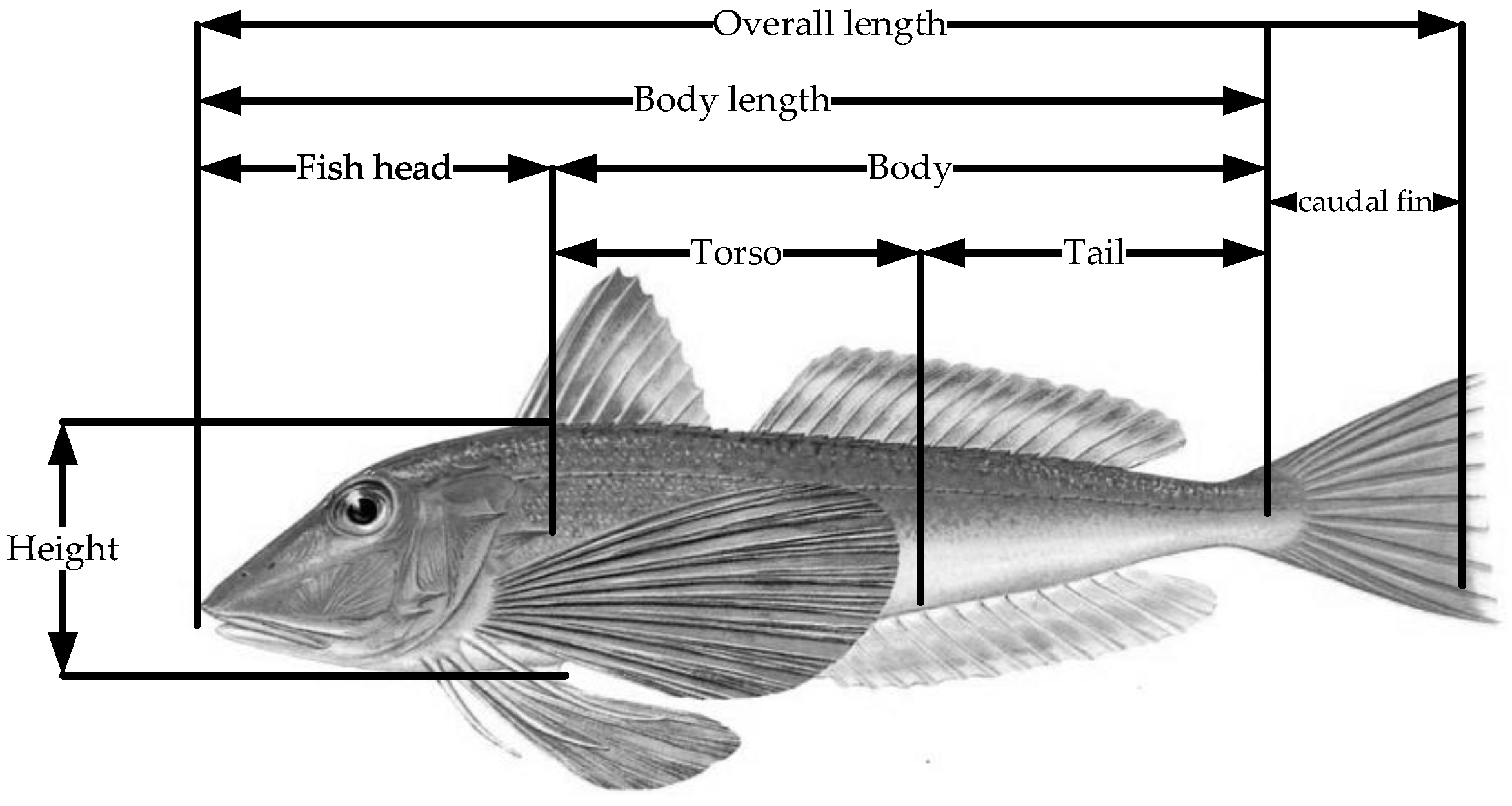
The greenfin fish, Pomfretidae, genus Greenfin, has a long, slightly laterally flattened body with a thick anterior region and a tapering posterior segment. The pectoral fins are long and broad, measuring 4.6–4.7-times the body height, 2.9–3.8-times the head length, and 5.4–5.5-times the tail length. When fully inflated, the pectoral fins measure around 1.8–1.9-times the body width and 0.4–0.5-times the body length. The bodily parameters are simplified equally based on the idea that functional mimicry is fundamental and physical mimicry is secondary. Greenfin fish move underwater primarily by water-striking from the back half of the fish with the caudal fin and bird-like water-skimming propulsion from the pectoral fins. The caudal fin propulsion mode of the bionic greenfin robot is similar to the body/caudal fin propulsion mode of conventional bionic fish robots. The pectoral fin’s water-skimming propulsion mode is identical to the flight-fluttering motion of birds such as hummingbirds, in which the thrust and lift are obtained by adjusting the angle of attack and skimming angle in real time to interact with the water current. The bionic greenfin fish robot designed in this paper has a pair of large pectoral fins, which lays the foundation for the pectoral fin water-skimming propulsion, and the efficiency of the propulsion mode of the tail fins swinging from side to side is also lower because of the larger pectoral fins, so the bionic greenfin fish robot studied in this research is mainly propelled by the pectoral fins, and the tail fins are responsible for realizing the steering and emergency stop function.

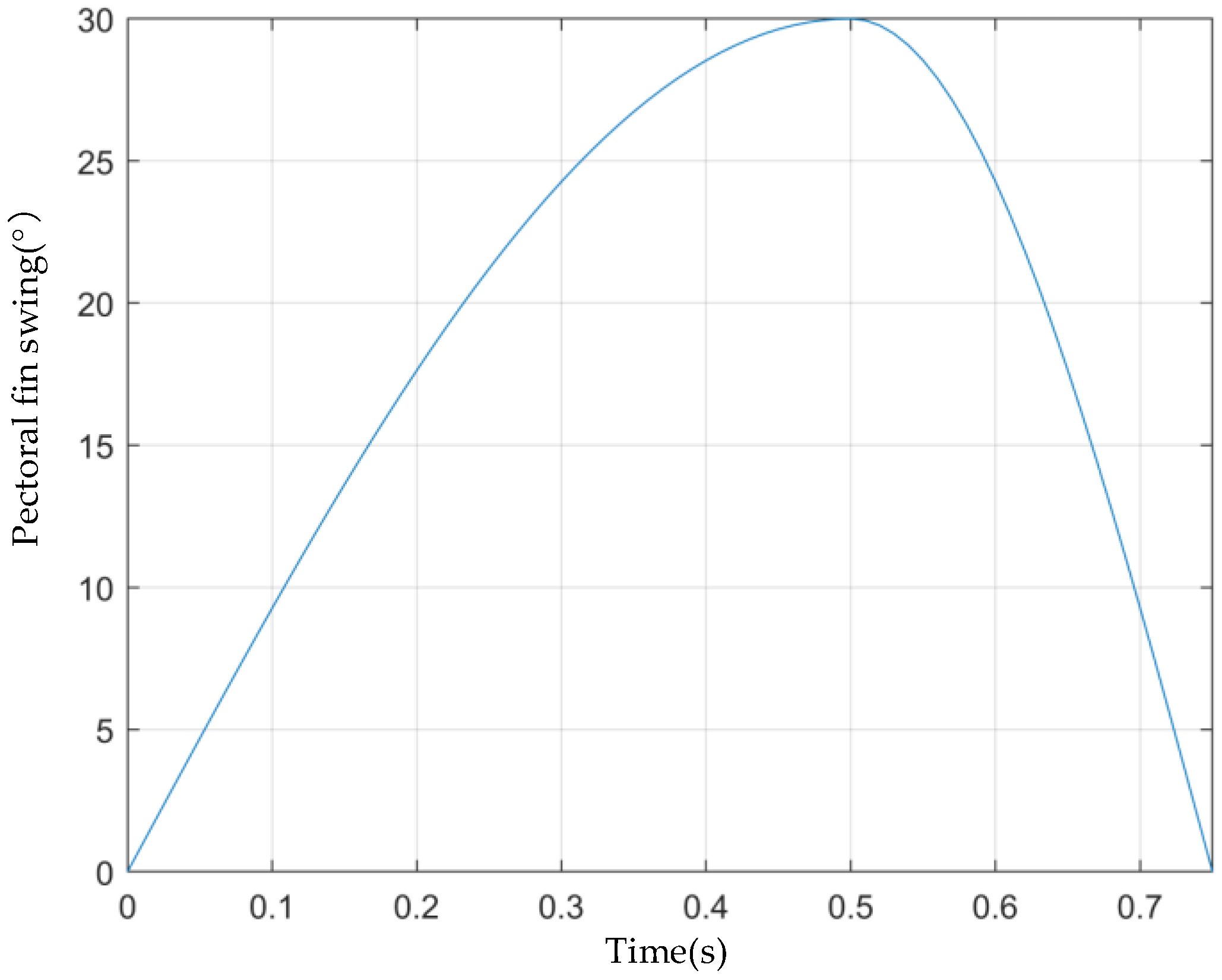
1. Pectoral fin propulsion mechanism: Generally, the sinusoidal signal can maintain a smooth transition in the switching of motion modes, and basically, the sinusoidal motion mode will be used for control when building the kinematic model of the pectoral fin. The kinematic modes of the pectoral fins are classified into three types: single-degree-of-freedom flutter motion, double-degree-of-freedom composite motion rotating around two axes, and three-degree-of-freedom composite motion rotating around three axes. The three-degree-of-freedom composite motions include the following: rocking wing motion around the y-axis, flutter motion around the x-axis, and forward and backward flutter motion around the z-axis. It can be expressed as

$$\left\{\begin{array}{l}{\varphi }_R={\varphi }_{RC}-{\varphi }_{R0}\cos (\omega t)\\ {\varphi }_F={\varphi }_{FC}-{\varphi }_{F0}\cos (\omega t+\Delta {\varphi }_F)\\ {\varphi }_{FL}={\varphi }_{FLC}-{\varphi }_{FL0}\cos (\omega t+\Delta {\varphi }_{FL})\end{array}\right.$$

(1)

In the above equation,

${\varphi }_R$, ${\varphi }_F$, ${\varphi }_{FL}$—Euler angles of pectoral fin anterior-posterior flutter, rocker flutter, and up-and-down flutter;

${\varphi }_{RC}$, ${\varphi }_{FC}$, ${\varphi }_{FLC}$—Mean values of pectoral fin anterior-posterior flutter, rocker flutter, and up-and-down flutter;

${\varphi }_{R0}$, ${\varphi }_{F0}$, ${\varphi }_{FL0}$—Amplitudes of pectoral fin anterior and posterior flutter, rocker flutter, and up-and-down flutter;

$\Delta {\varphi }_F$, $\Delta {\varphi }_{FL}$—Phase difference;

$\omega$—Angular velocity of motion.

The bionic fish robot uses pectoral fin propulsion, which is similar to that of birds. Just as hummingbirds and other birds flap their wings to fly, the pectoral fins of fish can realize a bird-like water-skimming motion by changing the oscillation angle of the pectoral fins and the angle of attack in real time.

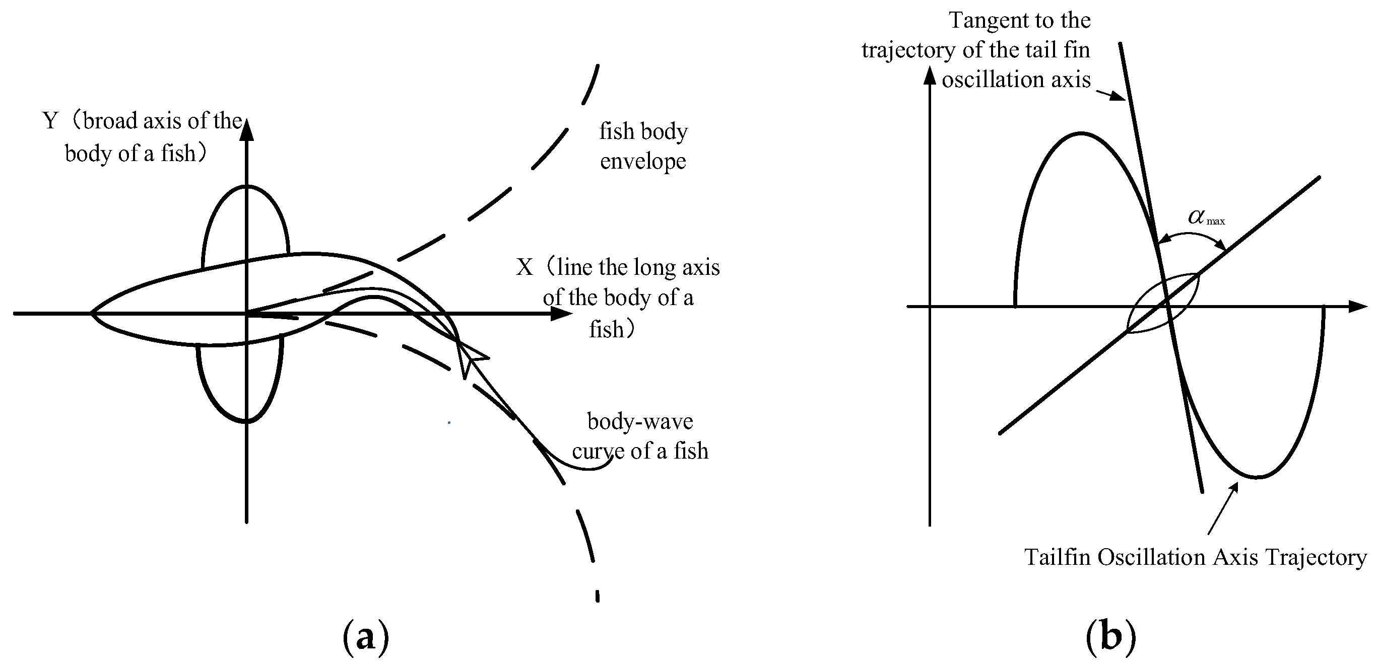
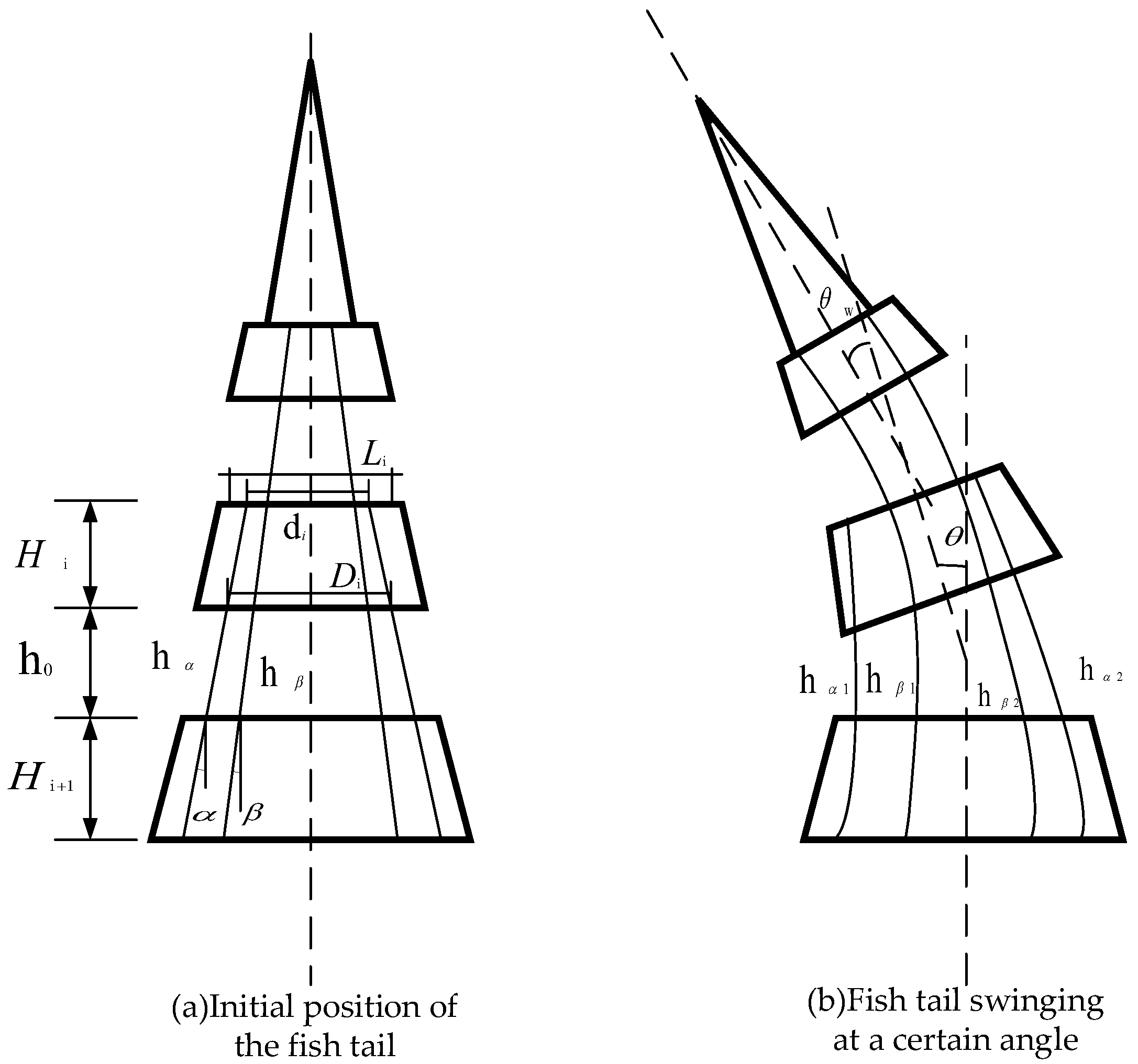
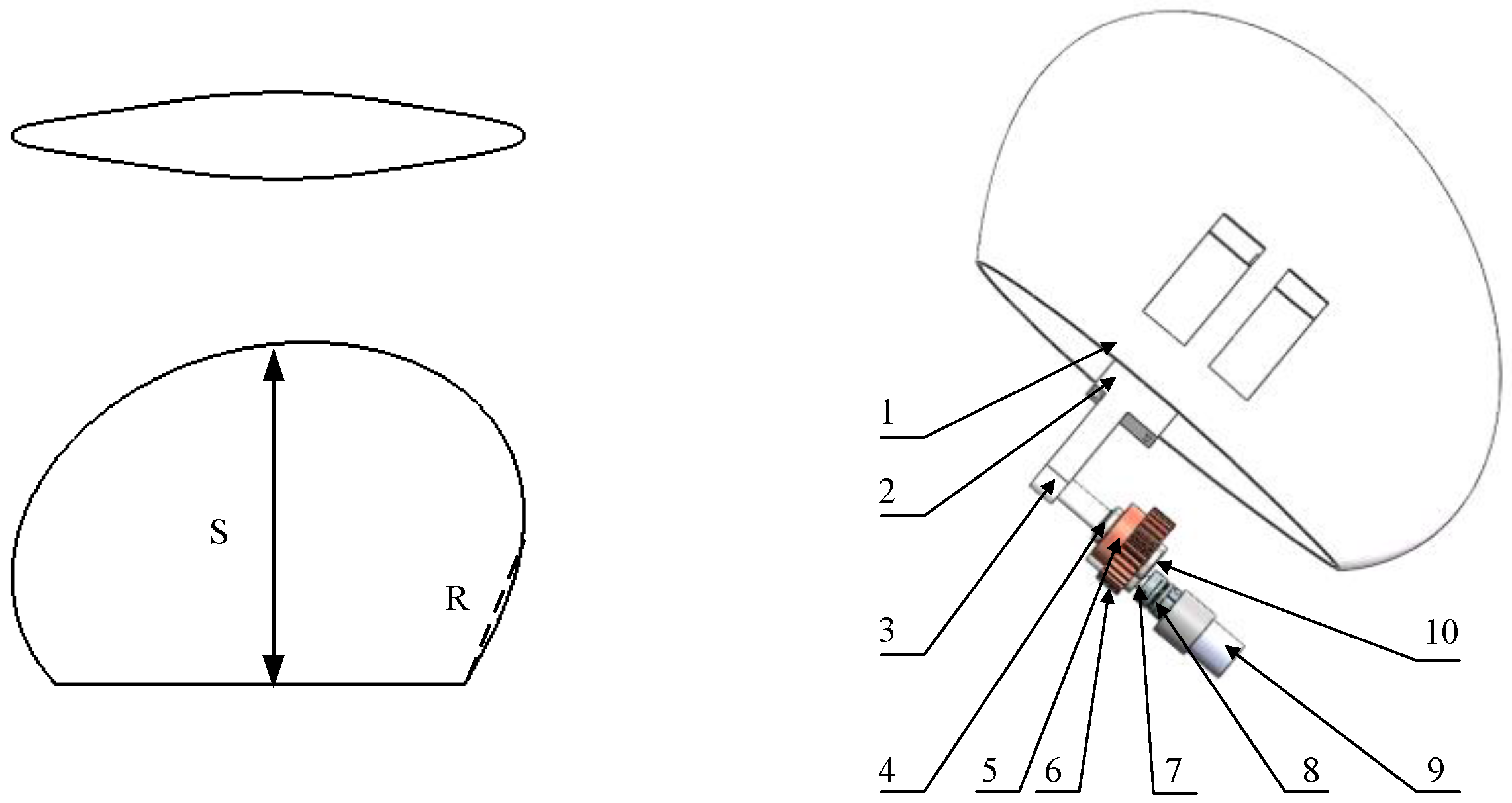
2. The caudal fin propulsion mechanism: The motion of a robotic fish mimicking a trevally plus crescent-shaped caudal fin pattern in the two-dimensional steady-state case can be decomposed into two parts: the fluctuation of the body of the fish and the composite motion of the tail fin driven by the body of the fish in an advection and its own oscillation. The specific curves and angles are shown in Figure 1.

The fish body wave equation can be viewed as a coupling of the fish wave amplitude envelope and a sinusoidal curve.

$$y_A(x,t)=(c_{1}x+c_2{x}^2)sin(k_{ytb}x+{\omega }_{ytb}t)$$

(2)

In the formula:

$y_A$—Transverse displacement of the fish body (in the direction of the wide axis of the fish body);

$x$—Axial position change in the fish body (direction of the long axis of the fish body);

$c_1$—Coefficients of the primary term of the wave amplitude envelope equation;

$c_2$—The coefficients of the quadratic terms of the wave amplitude envelope equation;

$\lambda$—The wavelength of the fish body wave, $k_{ytb}=2\pi /\lambda$;

${\omega }_{ytb}$—The frequency of the fish body wave, ${\omega }_{ytb}=2\pi f_{ytb}=2\pi /T$.

where the values of $c_1$ and $c_2$ are related to the swimming posture of the fish and the length dimension of the fish’s body, as well as the swimming speed of the fish. Their values determine the swing of the bionic fish’s body. The fish body wave equation determines the bionic fish’s mobility. The portion of the robotic body oscillations of fish bits usually reproduces the curve of the first 1/3 or so of the wavelength of the complete fish body wave. The motion of the caudal fin can be decomposed into an oscillation of the caudal fin and a flat motion of the caudal fin derived from the fish’s body wave drive. These two motions are not synchronized but have a certain phase difference. It has been shown that the propulsive efficiency is highest when the phase difference is at 90°.

The maximum strike angle ${\alpha }_{\max }$ is another major factor affecting the propulsive efficiency of the caudal fin. The strike angle α is the angle between the tangent of the trajectory line of the caudal fin oscillation axis and the centerline of the caudal fin at a certain point. When the maximum strike angle ${\alpha }_{\max }$ is 0°, the centerline of the caudal fin at a certain point coincides with the tangent to the trajectory line of the tail fin oscillation axis at that point. In this case, no propulsive force is generated by the oscillation of the caudal fin. Experience has shown that the propulsive force generated by the caudal fin gradually increases in the interval from 0° to 25° for the maximum water strike angle. As it increases to 30°, the caudal fin produces almost no propulsive force relative to the fish’s body, and beyond 40°, the caudal fin oscillates to impede the propulsion of the fish’s body.

When combined with the morphological characteristics of the greenfin fish, the larger pectoral fins provide a guarantee for the pectoral fin propulsion mode, but they also produce a higher traveling resistance. The tail fin propulsion mode for the bionic greenfin fish robot’s propulsion speed and propulsion efficiency is much lower than the pectoral fin propulsion mode. As a result, the bionic fish robot designed in this project is primarily based on the pectoral fin’s water-skimming propulsion mode with a higher propulsion speed, while the caudal fin is primarily responsible for steering and stopping, completing the overall design of the bionic greenfin fish robot. Based on the morphological and structural composition of the greenfin fish, the bionic greenfin fish robot as a whole can be divided into four parts: head, body, pectoral fins, and caudal fins. Based on geometric integration and accuracy, function sharing, supplier capability, similarity of design or production technology, centralized modification, suitability for diversification, standardization, and convenience of association, the corresponding module elements are divided into corresponding sections, and all possible clustering schemes are considered. The division of specific modules is shown in Figure 2.

The bionic greenfin fish robot designed in this project is oriented to the water quality of aquaculture ponds and underwater environment monitoring. The bionic robot fish needs to be able to detect water quality and swim flexibly. The role of detecting water quality requires the fish to be able to detect acidity, alkalinity, and pollutant concentration in various water settings, which necessitates the use of a detection module as well as an information-gathering module. Flexible swimming necessitates that the robot fish accelerate, decelerate, steer, hover, and perform other behaviors, such as pleasing fish, all of which require the use of an execution module, power module, and control module.

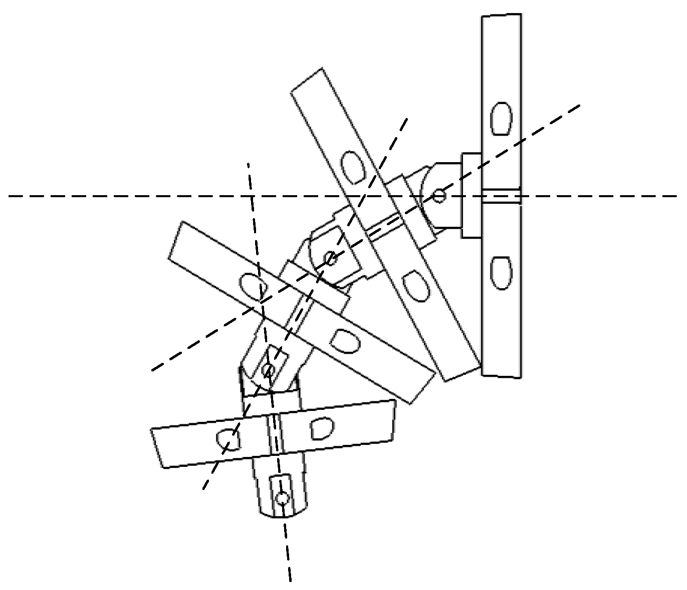
When combined with the morphological characteristics of the greenfin fish, the larger pectoral fins provide a guarantee for the pectoral fin propulsion mode, but they also produce a higher traveling resistance. The tail fin propulsion mode for the bionic greenfin fish robot’s propulsion speed and propulsion efficiency is much lower than the pectoral fin propulsion mode. As a result, the bionic fish robot designed in this project is primarily based on the pectoral fin’s water-skimming propulsion mode with a higher propulsion speed, while the caudal fin is primarily responsible for steering and stopping, completing the overall design of the bionic greenfin fish robot. The function of the drive module is to be realized by the pectoral fins and the caudal fins, and its shape, angle, and movement mode need to be modified many times, so the drive module is put into the body of the fish, it can be used as the cabin of the motion control system, and it is convenient to centralize the modification. The motion of the greenfin fish is mainly realized by the motion of the three parts of the pectoral fin, tail, and caudal fin, and the three actuator modules of the pectoral fin, tail, and caudal fin are designed as the corresponding motion actuators according to the design task.

According to the motion control objective of the bionic fish, the hardware of the control system is designed and planned, which includes the selection of the control chip, the selection of the communication mode, the selection of the power source, and the design of the floating and sinking mechanism, etc. The overall structure of the bionic greenfin fish robot is shown in Figure 3.

2.2. Fishtail Kinematic Analysis and Control Analysis

2.2.1. Modeling and Analysis of Caudal Fin Kinematics of Fish Tails

The fishtail part of the bionic greenfin fish robot is mainly composed of two parts: the flexible skeleton and the fishtail unit. The flexible skeleton and the rigid support in the fishtail unit are connected together by screws. The bending elasticity of the flexible skeleton determines the oscillation performance of the fishtail part, and it has to be less likely to break when the circular deformation occurs under force. A TPU thermoplastic polyurethane elastomer was chosen for the flexible skeleton. The fishtail structure is shown in Figure 4:

This paper uses a kinematic model-based control method for the tail fins, with the drive method being a tiller drive, thus pulling the rope to control the oscillation of the tail fin of the fish. In order to calculate the relationship between the control parameters of the fishtail fin and the rotation angle of the rudder, the paper simplifies the design parameters of the fishtail fin of the cable-pulling mechanism and gives a simplified schematic diagram of the structure, as shown in Figure 5. The diagram (a) indicates the initial position, while the diagram (b) indicates a certain angle of relative rotation. $H_i$ is the height of the fishtail unit; $h_0$ is the initial joint gap; $h_{\alpha }$ is the initial line length of the fishtail through the joint gap; $h_{\beta }$ is the initial line length of the caudal fin through the joint gap; $L_i$ is the length of the elliptical short axis on the rear surface of the fishtail unit; $d_i$ is the center distance between the two line holes on the rear surface of the fishtail unit; $D_i$ is the center distance between the two line holes on the front surface of the fishtail unit; $\alpha$ is the angle of inclination of the fishtail pulling line hole; $\beta$ is the angle of inclination of the fishtail pulling line hole; $\theta$ is the fishtail joint; ${\theta }_w$ is the angle of rotation of the caudal fin.

Most kinematic models of fish are based on the elongated body theory proposed by Lighthill, according to which the fish body wave is a system of traveling waves of increasing amplitude. Lighthill proposed a combination of polynomials and sinusoidal curves to describe the caudal fin fluctuations of the fish tail [19].

$$y_A(x,t)=(c_{1}x+c_2{x}^2)sin(k_{ytb}x+{\omega }_{ytb}t)$$

(3)

According to the fish body wave formula, it is deduced that the swing of the tail fin also conforms to the sine law. According to its derivation, for the five joints of the paper, the structure of the caudal fin of the fishtail conforms to the following equation:

$$\left\{\begin{array}{l}{\mathrm{\Phi }}_1(t)=k_2(1-k_1){\mathrm{\Phi }}_{1\max }+k_1{\mathrm{\Phi }}_{1\max }\sin (2\pi f)\\ {\mathrm{\Phi }}_2(t)=k_2(1-k_1){\mathrm{\Phi }}_{2\max }+k_1{\mathrm{\Phi }}_{2\max }\sin (2\pi f+{\mu }_1)\\ {\mathrm{\Phi }}_3(t)=k_2(1-k_1){\mathrm{\Phi }}_{3\max }+k_1{\mathrm{\Phi }}_{3\max }\sin (2\pi ft+{\mu }_2)\\ {\mathrm{\Phi }}_4(t)=k_2(1-k_1){\mathrm{\Phi }}_{4\max }+k_1{\mathrm{\Phi }}_{4\max }\sin (2\pi ft+{\mu }_3)\\ {\mathrm{\Phi }}_5(t)=k_2(1-k_1){\mathrm{\Phi }}_{5\max }+k_1{\mathrm{\Phi }}_{5\max }\sin (2\pi ft+{\mu }_4)\end{array}\right.$$

(4)

The structure of the caudal fin of the fishtail is shown in Figure 6. The dotted lines in the figure depict the centerlines of each joint:

2.2.2. Fishtail Tail Fin Steering and Emergency Stop Control Analysis

Through the analysis of the wave curve of the fish body, we find that the swing of the tail fin of the fish can also be controlled by a sinusoidal law. The steering control of the caudal fin can be thought of as the control of semi-propulsive motion, which creates both lateral and thrust force throughout the swinging process. The caudal fin generates substantially more lateral force than the pectoral fin, resulting in a steering torque that offers a power basis for the bionic robot’s steering action. The existence of the incoming force causes the bionic robot to follow forward motion while steering, affecting the steering function. When there is a positive phase difference between the fishtail and the caudal fin, meaning that the caudal fin swing lags behind the fishtail swing, the bionic robot’s effective work time in one swing cycle is increased, resulting in a greater propulsive force. As a result, when the bionic greenfin fish robot steers, the phase difference is set to zero degrees. Combining the simulation findings, take $k_2$ = 0,$k_1$ = 1, ${\Phi }_{1max}$ = 7.5°, ${\Phi }_{2max}$ = 15°, ${\Phi }_{3max}$ = 22.5°, ${\Phi }_{4max}$ = 30°, ${\Phi }_{5max}$ = 45°, ${\mu }_1$ = ${\mu }_2$ = ${\mu }_3$ = ${\mu }_4$ = 0°, $f$ = 1. We take half the period of the direct motion as the period of the steering motion and simulate it in MATLAB 2022b to obtain the curve of the change in the mid-axis of the tail fin of the fish in one cycle, as shown in Figure 7.

When there is a negative phase difference between the tail and the caudal fin, i.e., the oscillation of the tail lags behind the oscillation of the caudal fin, the bionic fish swims backward. Based on this observation and the context of the bionic robotic fish application, the fishtail caudal fin oscillates in a negative phase when an emergency stop is required to reduce displacement owing to the inertia of the body of the defensive robotic fish after stopping its motion.

According to the simulation results take $k_2$ = 0, $k_1$ = 1, ${\Phi }_{1max}$ = 7.5°, ${\Phi }_{2max}$ = 15°, ${\Phi }_{3max}$ = 22.5°, ${\Phi }_{4max}$ = 30°, ${\Phi }_{5max}$ = 45°, ${\mu }_1$ = ${\mu }_2$ = ${\mu }_3$ = 0, ${\mu }_4$ = 90°, $f$ = 1. The oscillation of the caudal fin leads the phase of the 90° oscillation of the fishtail. Simulations were carried out in MATLAB to obtain a curve of the change in the mid-axis of the caudal fin of the fishtail in one cycle, as shown in Figure 8.

2.3. Hydrodynamic Simulation Analysis of Tail Fin Steering Emergency Stop Performance

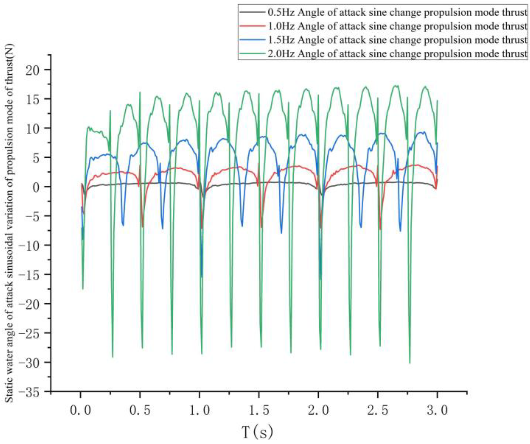
The application scenario for this thesis uses an aquaculture pond as an example, the water of the industrialized aquaculture pond circulates, the underwater flow rate of the aquaculture pond is typically around 6–8 cm/s, and the water surface flow rate is quicker. Under comprehensive consideration, we investigate the influence of the sinusoidal variation in the angle of attack on the propulsive movement of the bionic green finfish robot, which is initiated under the incoming flow rate. The effects of thrust, lift, and propulsive velocity are examined.

The width of the fish body is determined comprehensively according to the proportion of the size parameters of the greenfin fish and the need to minimize the size of the internal space. In this paper, we take a fish body height of 200 mm, a fish body width of 172 mm, a fish body length of 920 mm, a head length of 317 mm, a tail length of 306 mm, a tail length of 170 mm, a pectoral fin width of 319 mm, and a pectoral fin length of 438 mm. The numerical simulation of this model is carried out by using Fluent. Finite-element analysis is verified, the fluid material is selected as the default setting of water-liquid in the material library, the underwater turbulence state is considered, the standard form of the equation of the turbulence model k-ε is selected, and the non-equilibrium wall function is used to deal with the turbulence in the near-wall region. The boundary condition inlet velocity is set to 0.5 m/s. The SIMPLEC algorithm is used for pressure–velocity coupling, and the diffusion term is represented by a second-order center difference format. The static domain velocity inlet and velocity amplitude at the start are set to 0.1 m/s. Other settings remain constant.

The tail fin of the bionic greenfin robot designed in this paper is mainly used for steering and emergency stop functions, and the steering performance of the tail fin is reflected by the difference between the lateral forces on the fish body and the tail fin when the fishtail is swinging. The fishtail steering relies on the one-way oscillation of the fishtail, which corresponds to the left and right oscillation frequencies of 0.5 Hz, 1 Hz, 1.5 Hz, and 2 Hz, respectively, 1 Hz, 2 Hz, 3 Hz, and 4 Hz. In the simplified model, the tail joint near the fish’s body is swung at an angle of 15°, the tail fin swing is chosen to be 35°, and the simulation time is 3 s. Using 2 Hz as an example, the fishtail steering oscillation takes a value of 0.5 s for one cycle, and the lateral force stabilizes after approximately one cycle. The instantaneous pressure clouds for 0.01 s, 0.1 s, 0.2 s, 0.3 s, 0.4 s, and 0.5 s are shown in Figure 9. The graphic shows the force on the fish’s body, particularly its tail, during a cycle.

The change in lateral forces on the pectoral and caudal fins of the fish at each of the four frequencies is shown in Figure 10.

As can be seen in Figure 10, the lateral forces on the pectoral fins and caudal fins of the fish at the four frequencies also show a cyclic variation within 1 s. By analyzing the variation in the lateral forces on the pectoral fins and caudal fins of the fish within 1 s, the steering performance of the bionic greenfin fish robot at different frequencies can be analyzed.

The average lateral force on the pectoral fins of the fish increased with frequency, but the work done by the average lateral force at 1 s was zero, which was attributed to the bigger size of the pectoral fins and the higher inertia of the bow rotation. The average lateral force on the caudal fin increased faster with increasing frequency in 1 s. The average lateral force on the caudal fin at different frequencies is shown in Figure 11.

Figure 11 shows that frequency has a significant effect on the average lateral force delivered to the caudal fin of the fish in 1 s. At a frequency of 1 Hz and a swing of 35°, the fish swings once in 1 s and the average lateral force generated is so small that it is almost impossible to achieve the steering function; however, at a frequency of 4 Hz, the machine fish can swing 4 times in 1 s and the average lateral force generated in 1 s is more than 10 N, indicating a superior steering performance.

The tail fin swing is another important component that influences the fish’s tail fin steering performance. The frequency is set at 2 Hz, the tail joint turning angle near the body of the fish is 15° and the tail fin joint turning angles are 35°, 40°, 45°, 50°, 55°, and 60° to analyze the effect of the tail fin swing on the tail fin steering performance.

Taking the 40° swing as an example, the time for one cycle of the fishtail steering swing is 0.5 s, and the instantaneous pressure clouds for 0.01 s, 0.1 s, 0.2 s, 0.3 s, 0.4 s, and 0.5 s in one cycle are shown in Figure 12.

Figure 12 shows that the force on the caudal fin of the fish tail was greater at 0.01 and 0.5 s, with dramatic and substantial fluctuations, but the force on the pectoral fin was less variable.

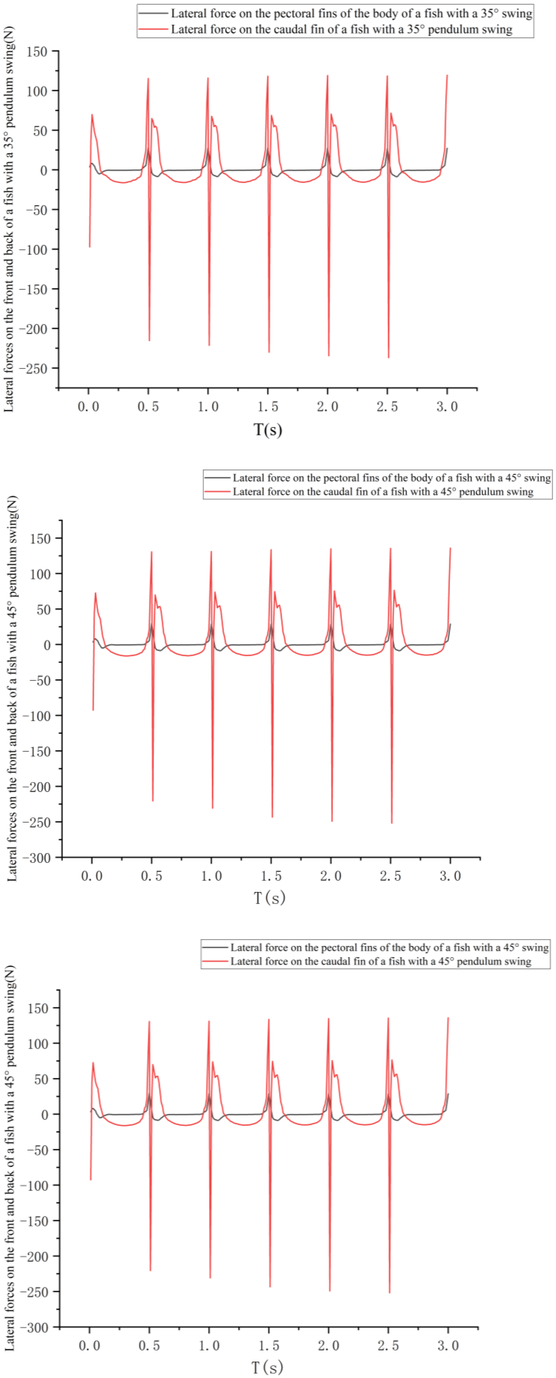
The lateral forces on the pectoral and caudal fins of the fish at different swing amplitudes are shown in Figure 13.

As can be seen in Figure 13, the lateral forces on the pectoral and caudal fins of the fish also vary periodically within 1 s at different caudal fin swings.

The average lateral force in 1 s on the pectoral fin of the fish also remained essentially around 0 for different caudal fin swings. The mean lateral force on the caudal fin increased with increasing caudal fin swing over 1 s. Figure 14 depicts the average lateral force on the caudal fin during various caudal fin swings.

From Figure 14, it is obtained that the average lateral force applied to the caudal fin of the fishtail in 1 s increases faster when the swing amplitude increases from 35° to 45°, then slows down after exceeding 45°. After exceeding 55°, the average lateral force supplied to the caudal fin of the fishtail in 1 s starts to drop significantly as the fishtail swing amplitude increases. When the bionic greenfin fish robot steering function is enabled with a swing frequency of 2 Hz and a tail fin swing amplitude of 45°, it reduces the rudder torque pressure and increases the service life while maintaining a better steering performance.

When the phase difference of caudal fin oscillations is positive, i.e., when the caudal fin oscillations lag behind those of the tail, the bionic fish swims normally; when the phase difference of caudal fin oscillations is negative, i.e., when the tail oscillations lag behind those of the caudal fin, the bionic fish swims in reverse.

Frequency is an important factor affecting the propulsion performance of the bionic fish robot. The emergency stop function requires a rapid stop in a short period of time, which is impossible to execute when the tail fin swing frequency is excessively low. This section investigates the effect of frequencies 1 Hz, 1.5 Hz, and 2 Hz on the emergency stop function of the bionic greenfin fish robot at 15° fish tail swing and 35° tail fin swing.

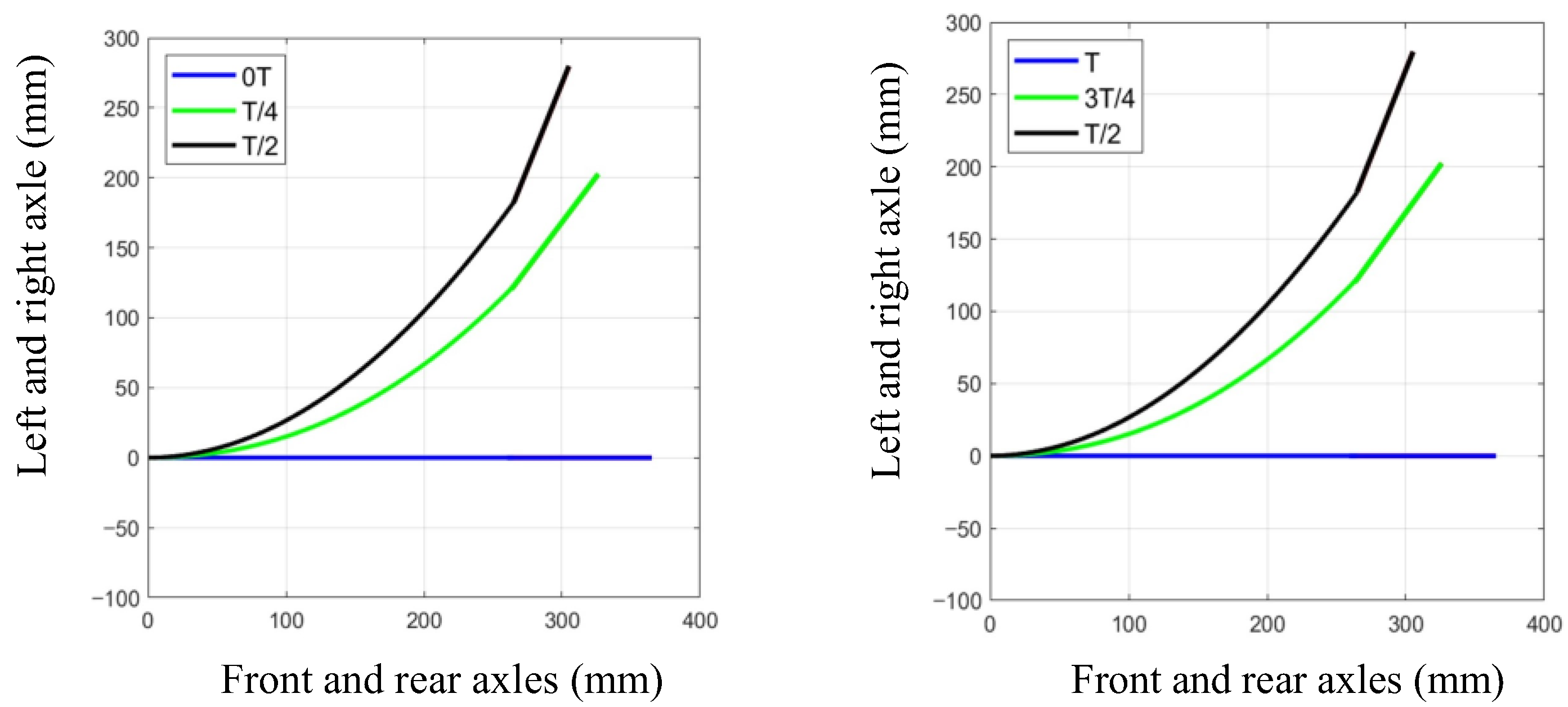
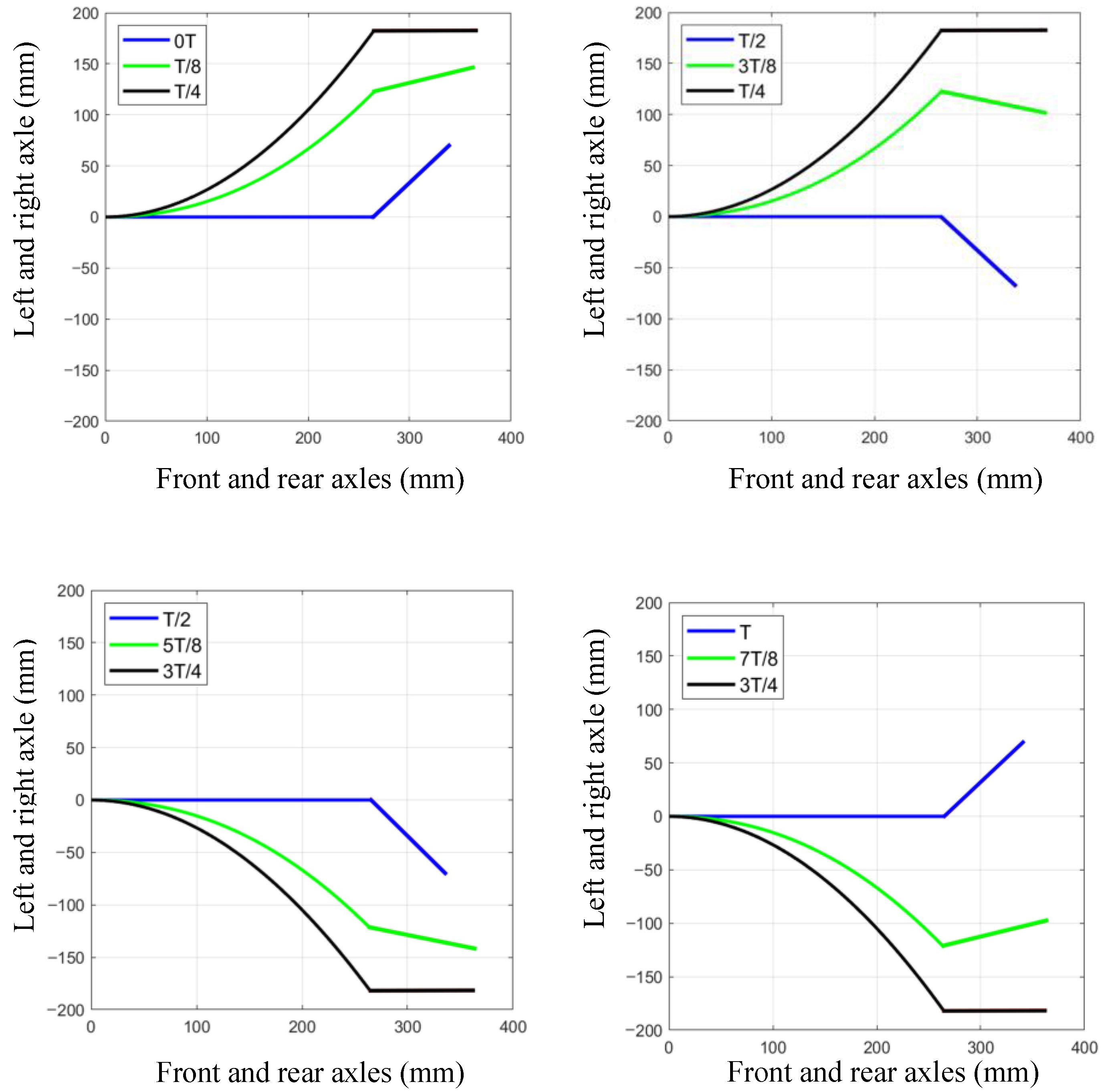
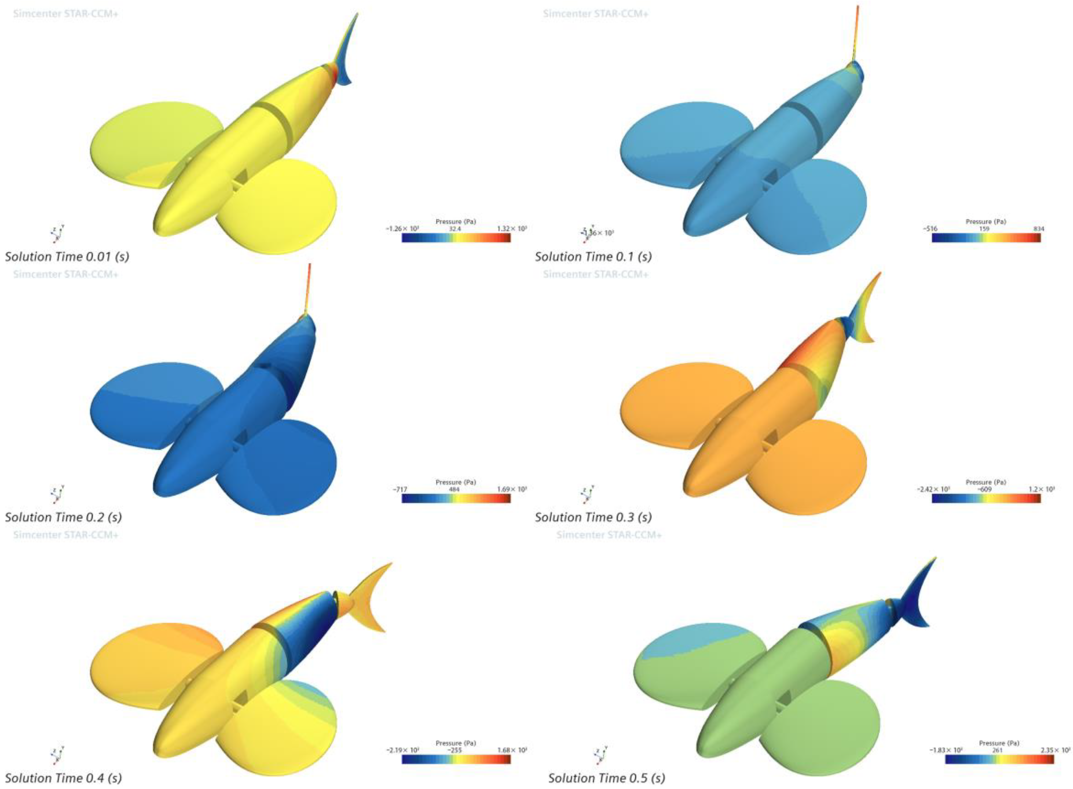
Using 2 Hz as an example, the tail fin negative phase oscillation time of one cycle is 0.5 s, and the surface pressure cloud of the bionic greenfin fish robot every 0.1 s is shown in Figure 15.

The propulsive force fluctuates with time, as seen in Figure 15, where the pressure is gradually transferred from the front to the back over one cycle of tail fin oscillation at a frequency of 2 Hz.

The thrust variation curves for the negative phase oscillation of the tail fin at different frequencies are shown in Figure 16.

As the frequency increases, so does the amplitude of the change in thrust caused by the tail fin’s negative phase oscillation, as well as the impulse in the direction of drag generated in one cycle.

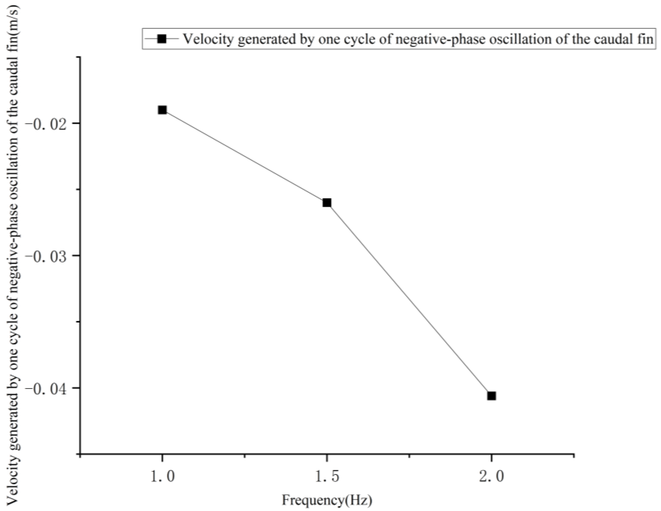
The velocity change curve generated by one cycle of negative phase oscillation of the tail fin at different frequencies is shown in Figure 17.

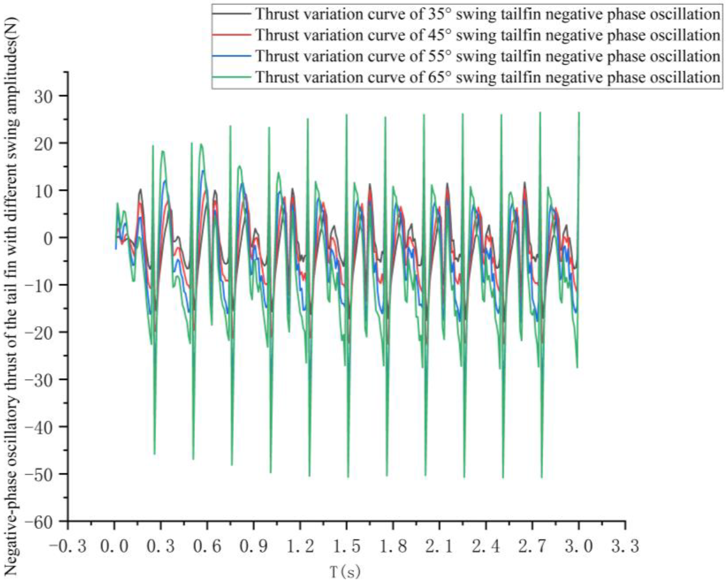
Tail fin swing amplitude is also a major factor in tail fin propulsion performance, as it is in the application of negative phase oscillation. This section investigates the effect on the negative phase oscillation performance of the tail fin at a 2 Hz oscillation frequency with a tail joint oscillation of 15° and tail fin joint oscillations of 35°, 45°, 55°, and 65°, respectively.

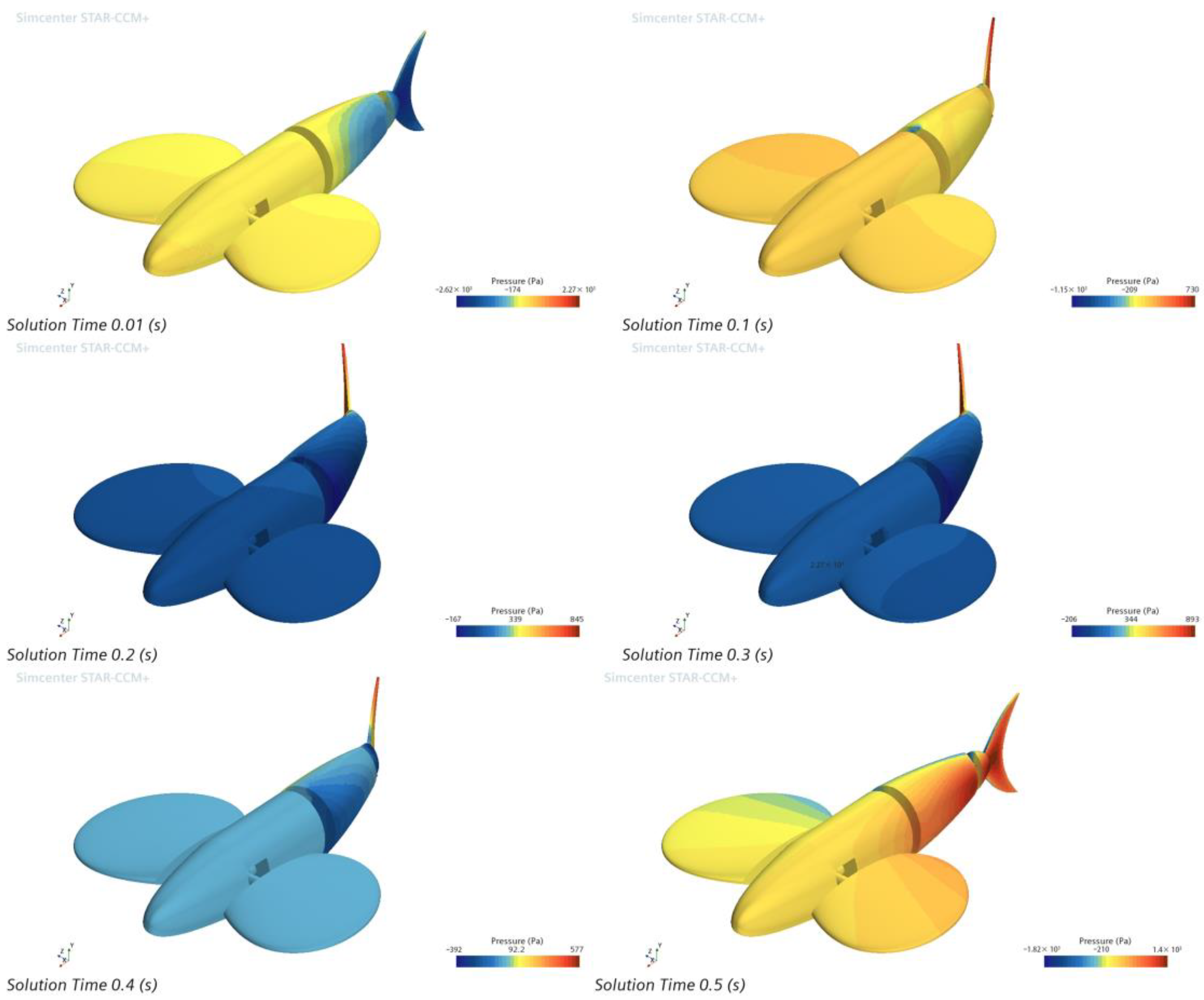
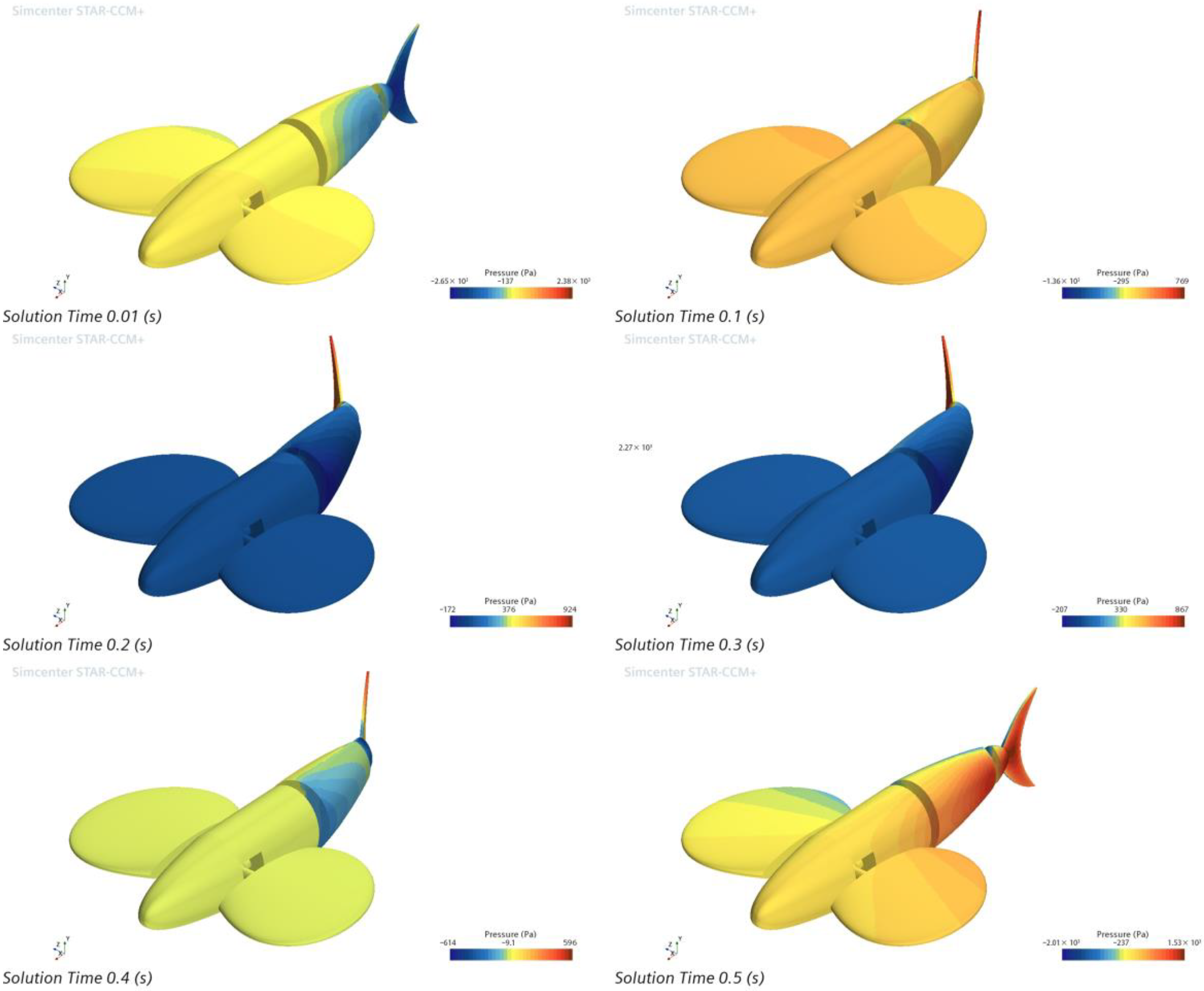
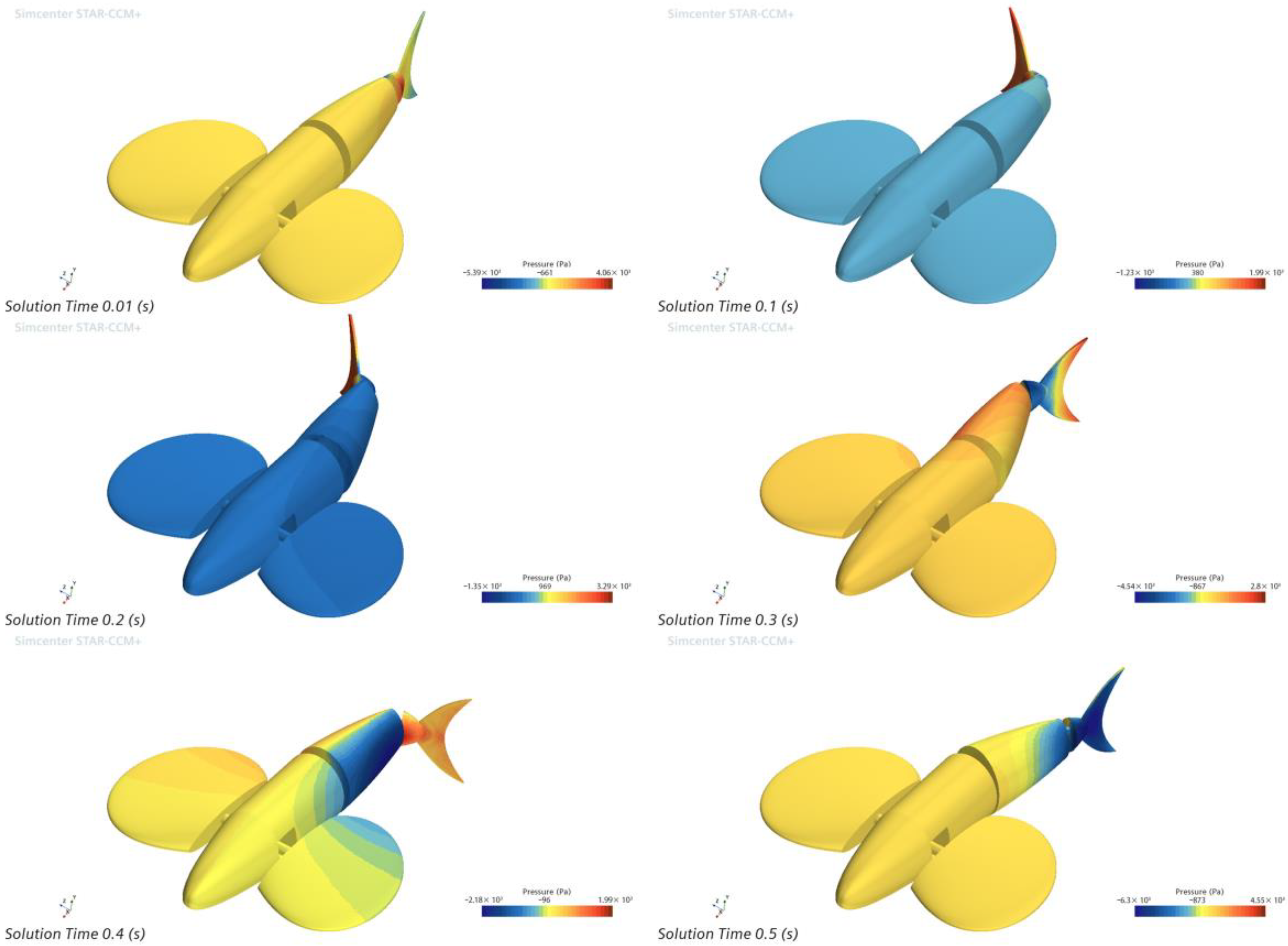
Taking the 65° tail fin swing as an example, the tail fin negative phase swing has a cycle time of 0.5 s, and the surface pressure cloud of the bionic greenfin fish robot every 0.1 s is shown in Figure 18.

Figure 18 depicts how, at a caudal fin negative phase swing of 65° and a frequency of 2 Hz, pressure is gradually transferred from the head to the rear over one cycle of caudal fin swing in the bionic greenfin fish robot, indicating a change in propulsive force over time similar to the change in Figure 15.

The curve of the change in thrust generated by the negative phase oscillation of the tail fin for the four tail fin oscillation amplitudes is shown in Figure 19.

Analysis of Figure 19 shows that as the tail fin swing increases, the amplitude of the change in thrust generated by the negative phase oscillation of the tail fin increases, and the impulse in the direction of drag generated in one cycle also increases.

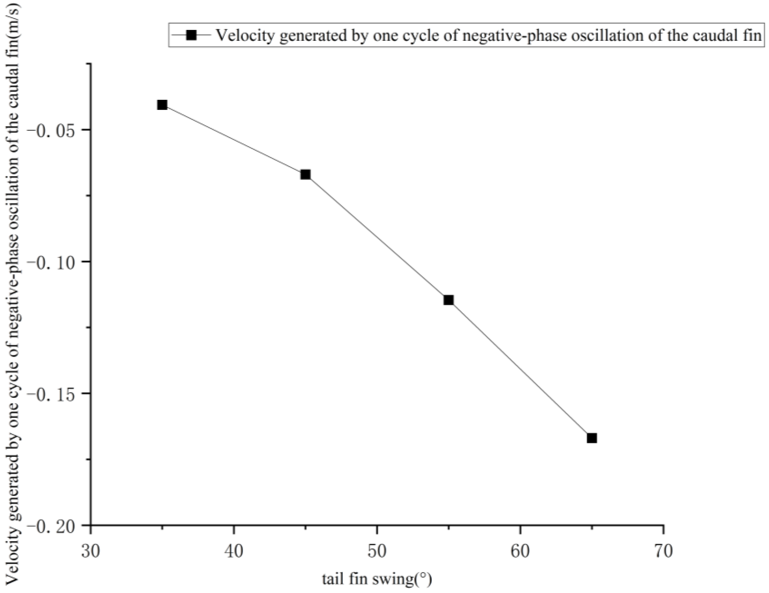
The velocity change curves produced by one cycle of negative phase tail fin swing for the four tail fin swing amplitudes are shown in Figure 20.

As the tail fin swing amplitude increases, the velocity generated in one cycle of negative phase tail fin swing also increases, with the fastest growth in velocity occurring between 45° and 55° of swing amplitude, and the increase in velocity slows down as the swing amplitude continues to increase beyond 55°. Considering the performance of the servo and its service life, the tail fin swing amplitude of the emergency stop function of the bionic greenfin fish robot in this paper was preferentially chosen to be 45°.

3. Fish Pectoral Fin Analysis and Design

3.1. Pectoral Fin Kinematic Modeling and Analytical Design

The design objectives for the pectoral fins of the bionic greenfin robot in this paper include a pectoral fin profile similar to that of a real greenfin; the ability of the greenfin to repeatedly strike the water longitudinally and to change the angle of attack of the pectoral fins in real time to achieve a “skimming” propulsive motion as the main source of power for the robot’s propulsion; and the ability to be used to balance the fish’s body and to assist in achieving a snorkeling mode of motion. The pectoral fin structure is shown in Figure 21.

Labels: 1—pectoral fin housing; 2—pectoral fin waterproof servo assembly; 3—pectoral fin connecting rod; 4—seal; 5—30 tooth large gear; 6—17 tooth small gear; 7—connecting shaft; 8—diaphragm coupling; 9—eccentric motor; 10—bearing.

Pectoral fin propulsion is the main method of propulsion for the bionic greenfin fish robot designed in this paper. The motion pattern of the pectoral fins of the bionic greenfin fish robot is determined by the pectoral fin motion actuator [20]. The pectoral fin motion actuator in this paper employs a DC motor and a gear drive. The DC motor powers the active gear, and hence the two driven gears. The driving gear’s angular displacement, angular velocity, and angular acceleration are the same as the pectoral fin’s. The main gear and both driven gears have a module of 2, the main gear has a $Z_1$ of 17 teeth, and both driven gears have a $Z_2$ of 30 teeth.

To make the movement pattern of the pectoral fins more efficient and stable, the up-and-down fluttering motion of the pectoral fins is sinusoidal [21].

$${\theta }_P={\theta }_{0P}+{\theta }_{P\max }\sin (2\pi f_{P}t)$$

(5)

In the formula:

${\theta }_P$—Pectoral fin flap amplitude (radian system);

${\theta }_{0P}$—Initial amplitude of pectoral fin flap (radian system);

${\theta }_{P\max }$—Maximum pectoral fin flap (radian system);

$f_P$—Pectoral fin flutter frequency.

By finding the derivative of the above formula over time, we obtain the rate of movement of the pectoral fin flaps ${\omega }_P$:

$${\omega }_P=2\pi f_P{\theta }_{P\max }\cos (2\pi f_{P}t)$$

(6)

The above formula continues with the derivative over time. To get the angular acceleration ${\alpha }_P$ of the pectoral fin flap,

$${\alpha }_P=-4{\pi }^2{f}_P^2{\theta }_{P\max }\sin (2\pi f_{P}t)$$

(7)

The fluttering motion of the pectoral fins is relatively similar to the fluttering motion of birds in that both change the angle of attack and the angle of oscillation during travel to gain forward thrust and upward lift. The mathematical model of the pectoral fin oscillation angle has been established. In this paper, we design the equations of motion for two modes of changing the angle of attack and verify the advantages and disadvantages of the two models of motion through hydrodynamic simulations in the latter part of the paper.

From the simulations, the most efficient motion and the highest lift-to-drag ratio of the bionic greenfin robot is obtained at an angle of attack of 10°, so 10° is chosen as the angle of attack variation for the pectoral fin propulsion motion.

The first mode of angle of attack change is similar to that of a hummingbird’s flight flutter, where the angle of attack is changed at the moment when the sweep angle (swing angle) of the hummingbird reaches its maximum or minimum value, and the equation of motion is

$${\theta }_{f1}=\left\{\begin{array}{l}200t,0\le t\le 0.05\\ 200({\displaystyle \frac{T}{4}}-t),{\displaystyle \frac{T}{4}}-0.05\le t\le {\displaystyle \frac{T}{4}}\\ 200(t-{\displaystyle \frac{T}{4}}),{\displaystyle \frac{T}{4}}\le t\le {\displaystyle \frac{T}{4}}+0.05\\ 200({\displaystyle \frac{T}{2}}-t),{\displaystyle \frac{T}{2}}-0.05\le t\le {\displaystyle \frac{T}{2}}\\ 200({\displaystyle \frac{T}{2}}-t),{\displaystyle \frac{T}{2}}\le t\le {\displaystyle \frac{T}{2}}+0.05\\ 200(t-{\displaystyle \frac{3T}{4}}),{\displaystyle \frac{3T}{4}}-0.05\le t\le {\displaystyle \frac{3T}{4}}\\ 200({\displaystyle \frac{3T}{4}}-t),{\displaystyle \frac{3T}{4}}\le t\le {\displaystyle \frac{3T}{4}}+0.05\\ 200(t-T),T-0.05\le t\le T\end{array}\right.$$

(8)

${\theta }_{f1}$ is the real-time angle of attack in this motion mode, which changes rapidly from 0 to 10° (−10°) in 0.05 s.

For the second, where the angle of attack moves in tandem with the pectoral fins and the motion of the angle of attack also follows the sine law and has the same frequency as the pectoral fin motion, the mathematical model for this mode of motion is

$${\theta }_{f2}={\theta }_{0f2}+{\theta }_{f2\max }\sin (2\pi f_{P}t)$$

(9)

In the formula:

${\theta }_P$—Amplitude of change in angle of attack (radian system);

${\theta }_{0f2}$—Initial amplitude of the angle of attack (in radians);

${\theta }_{f2\max }$—Maximum amplitude of change in angle of attack (radian system);

$f_P$—Pectoral fin flutter frequency.

The bionic greenfin robot swims in an “M”-shaped up-and-down motion, and when it stops abruptly, there is often a degree of displacement error owing to inertia. As a result, when the robot reaches the established monitoring position, its depth position may be higher or lower than the established water surface, and the mounted camera is smaller due to the hardware, so a larger depth error may affect the underwater image monitoring task. Traditional bionic fish robots change their depth by adjusting the center of gravity or the angle of attack of the pectoral fins while swimming. When the robot fish swims into a narrow or densely populated area, the small space will have a great impact on the way the robot fish changes its position and depth during swimming.

The bionic greenfin robot designed in this paper can flap slowly in the first 2/3 of a cycle and rapidly in the second 1/3 of a cycle. Among other things, the longitudinal lifting motion helps the robot fish to make monitoring position adjustments and to snorkel in tight spaces. The longitudinal rocking motion around the center of gravity allows the robot fish to quickly change its snorkeling angle in a short time and adjust its longitudinal rocking attitude for fast snorkeling.

The paper is designed to adjust the position of the center of gravity to the vicinity of the pectoral fin rotation axis by means of two front and rear screw slides, which enable the monitoring position adjustment function of the bionic greenfin fish robot in the near vertical direction by means of uneven up-and-down fluttering wings.

The pectoral fin kinematic model that implements this function is

$${\theta }_{\mathrm{s}}=\left\{\begin{array}{l}{\theta }_{\mathrm{smax}}\sin ({\displaystyle \frac{3}{4}}\pi f_{s}t),0\le t\le {\displaystyle \frac{2}{3}}T\\ {\theta }_{\mathrm{smax}}\sin ({\displaystyle \frac{3}{2}}\pi f_{s}t),{\displaystyle \frac{2}{3}}T\le t\le T\end{array}\right.$$

(10)

where ${\theta }_{\mathrm{s}}$ is the real-time flutter angle in the monitored position-adjusted flutter motion mode; ${\theta }_{\mathrm{smax}}$ is the flutter amplitude in the monitored position-adjusted flutter motion mode; and $f_s$ is the flutter frequency in the monitored position-adjusted flutter motion mode.

Using a 30° flutter amplitude, 1.33 Hz flutter frequency, and upper flutter motion as an example, the simulation curve of the change in pectoral fin angle for one cycle of flutter in MATLAB is shown in Figure 22.

The average lift generated by one cycle of the bionic greenfin fish robot flutter with the displacement in the direction of lift is

$$F_{pyyacg}={\displaystyle \frac{1}{T}}{\displaystyle \underset{0}{\overset{T}{\int }}{F}_{pyyi}dt}$$

(11)

$$s_{pyy}={\displaystyle \frac{T}{2m}}{\displaystyle \underset{0}{\overset{T}{\int }}{F}_{pyyi}dt}$$

(12)

where $F_{pyyi}$ is the instantaneous lift force acting on the center of gravity at each time point of the flutter motion, $T$ is the period of motion, and $m$ is the mass of the bionic greenfin fish robot.

Similarly, the displacement in the direction of the thrust generated by one cycle of the fluttering wings of the bionic greenfin fish robot is

$$s_{pyx}={\displaystyle \frac{T}{2m}}{\displaystyle \underset{0}{\overset{T}{\int }}{F}_{pyxi}dt}$$

(13)

where $F_{pyxi}$ is the instantaneous thrust acting on the center of gravity at each time point of the flutter motion.

The angle of transverse rocking generated by one cycle of the bionic greenfin robot flap is

$${\theta }_{xq}={\displaystyle \frac{L\sin {\theta }_{L}T{\displaystyle \underset{0}{\overset{T}{\int }}{F}_{xqi}dt}}{2J_{zy}}}$$

(14)

where $F_{xqi}$ is the instantaneous lift force acting on the pectoral fin at each point in time of the flutter motion; $L$ is the distance from the center of gravity of the pectoral fin to the center of gravity of the bionic greenfin fish robot; ${\theta }_{xq}$ is the angle between the axis of the pectoral fin rotation arm and the line connecting the center of gravity of the pectoral fin and the center of gravity of the bionic greenfin fish robot; $J_{zy}$ is the longitudinal rocking moment of inertia.

3.2. Hydrodynamic Simulation Analysis of Pectoral Fin Swept Water Propulsion Performance

As the pectoral fin skimming propulsion is perfectly symmetrical on the left and right sides, the study of the hydrodynamic performance of the pectoral fin skimming motion of the bionic greenfin fish robot focuses on the thrust and lift forces obtained by the bionic greenfin fish robot in one cycle.

The impulse and thrust obtained in the direction of thrust during one cycle of the pectoral fin skimming motion of the bionic greenfin fish robot is

$$I_{LX}={\int }_0^T{F}_{LX}dt$$

(15)

$$F_{LX}={\displaystyle \frac{1}{2}}{C}_{LX}\rho S_L{V}_L$$

(16)

where $I_{LX}$ is the impulse in the direction of thrust obtained by the bionic greenfin robot during one cycle of the pectoral fin skimming motion; $F_{LX}$ is the thrust obtained by the bionic greenfin robot at one moment of the pectoral fin skimming motion; $C_{LX}$ is the coefficient of thrust obtained by the bionic greenfin robot at one moment of the pectoral fin skimming motion; $\rho$ is the fluid density; $S_L$ is the area of the bionic greenfin robot’s headwater; $V_L$ is the headwater velocity of the bionic greenfin robot. From the momentum theorem, we have

$$p_{LX}=I_{LX}={\int }_0^T{F}_{LX}dt=m{\nu }_1-m{\nu }_0$$

(17)

where $p_{LX}$ is the momentum gained by the bionic greenfin robot in the direction of thrust during one cycle of the pectoral fin “skimming” motion; $m$ is the mass of the bionic greenfin robot; $v_1$ is the swimming speed of the bionic greenfin robot in the direction of thrust after one cycle; $v_0$ is the initial speed of the bionic greenfin robot.

Since $v_0=0$, we have

$$v_1={\displaystyle \frac{1}{2m}}{\displaystyle \underset{0}{\overset{T}{\int }}{C}_{LX}\rho S_L{V}_L}dt$$

(18)

Similarly, the lift force obtained by the bionic greenfin robot during one cycle of the pectoral fin “skimming” motion and the velocity in the direction of the lift force are

$$F_{LY}={\displaystyle \frac{1}{2}}{C}_{LY}\rho S_L{V}_L$$

(19)

$$v_2={\displaystyle \frac{1}{2m}}{\displaystyle \underset{0}{\overset{T}{\int }}{C}_{LY}\rho S_L{V}_L}dt$$

(20)

where $F_{LY}$ is the lift force obtained at a given moment of the pectoral fin “skimming” motion; $C_{LY}$ is the lift force coefficient obtained at a given moment of the pectoral fin “skimming” motion; $v_2$ is the velocity of the bionic greenfin robot swimming in the direction of lift after one cycle.

Hydrodynamic simulation of the lift and drag forces on the pectoral fins of a bionic greenfin fish robot at different angles of attack based on Fluent 2022.

The paper uses Fluent simulations to obtain the lift, drag, and lift resistance at angles of attack of 0°, 10°, 20°, 30°, 40°, and 45°, as shown in Figure 23.

The next step is to investigate the effect of different angles of attack on the “water-skimming” propulsion mode of the bionic greenfin robot at a flutter amplitude of 30° at a frequency of 2 Hz. To simplify the calculations, the paper simulates half of the “water-skimming” propulsive motion of the fish. The grids are shown in Figure 24.

In order to make the movement pattern of the pectoral fins more efficient and stable, the up-and-down fluttering motion of the pectoral fins uses sinusoidal motion. Set the field function of the pectoral fin oscillation motion with respect to the sinusoidal variation in the angle of attack as

$${\theta }_P={\theta }_{pmax}\sin (2\pi f_{P}t){\displaystyle \frac{\pi }{180}}$$

(21)

$${\theta }_f={\theta }_{f\max }\sin (2\pi f_{P}t){\displaystyle \frac{\pi }{180}}$$

(22)

where ${\theta }_P$ is the real-time arc of the pectoral fin swing; ${\theta }_{pmax}$ is the amplitude of the pectoral fin swing; $f_P$ is the frequency of the pectoral fin swing and angle of attack change; ${\theta }_f$ is the real-time arc of the angle of attack; ${\theta }_{f\max }$ is the amplitude of the angle of attack change.

In the Fluent simulation, the pectoral fins and the fluid computational domain model are established. The fluid computational domain model is mostly square, and the naming selection determines the velocity inlet and pressure outlet; however, the boundaries of the pectoral fins cannot be too close to the six boundaries of the rectangular fluid computational domain, and the pectoral fins should be kept as close to the center of the flow field as possible. At the same time, the mesh division is the most essential component of the Fluent simulation computation. Based on prior experience, the expansion layer is added to the mesh division, resulting in the pectoral fin edge mesh being separated into numerous layers.

According to the analysis of the simulation results, the angle of attack exceeds 45° and the lift-to-drag ratio of the pectoral fin is close to 1. Therefore, the paper chose 10°, 20°, 30°, and 40° as the angle of attack variables to be studied. Specific relationships are shown in Figure 25.

The simulation results are shown in Figure 25 and Figure 26: the bionic greenfin robot shows periodic symmetry in lift force for all four angles of attack variations, and the pectoral fin “skimming” propulsion mode shows an up-and-down rocking propulsion state.

The change in propulsion velocity resulting from one cycle of pectoral fin “skimming” at different angles of attack is shown in Figure 27.

In the direct propulsion mode, the preferred angle of attack change is 10°, and the angle of attack change can be increased to obtain a higher propulsion speed when a larger incoming current is encountered.

The frequencies of 0.5 Hz, 1 Hz, 1.5 Hz, and 2 Hz were used to study the effect of frequency on the thrust and propulsion speed of the bionic greenfin robot in the “water-skimming” propulsion mode. The simulation results are shown in Figure 28.

The velocity change curve is shown in Figure 29.

The effect of different flutter amplitudes on the pectoral fin propulsion performance of the bionic greenfin fish robot at 2 Hz frequency with a 10° sinusoidal variation in the angle of attack was selected as the swing angle oscillation variable for the study, and the simulation results are shown in Figure 30.

As shown in Figure 31, with the increase in the pectoral fin swing amplitude, the speed under the “-skimming” propulsion motion of the bionic greenfin robot also increases, and the propulsion speed increases at the highest multiplier when the swing amplitude increases between 20° and 30°. Considering the practical application, the pectoral fin “skimming” propulsion mode with a pectoral fin swing of 30° requires less motor drive and can maintain a good swimming efficiency and propulsion speed.

3.3. Simulation Analysis of the Effect of Uneven Pectoral Fin Flutter on Monitoring Position Adjustment

The pectoral fins move vertically by fluttering unevenly up and down. When there is a depth error between the position of the bionic greenfin fish robot and the monitored position, its position adjustment at smaller depth errors can be achieved by uneven fluttering of the pectoral fins. This section investigates the influence of the frequency and amplitude of the uneven flutter of the pectoral fin on its flutter displacement through simulation to confirm the viability of its monitoring position adjustment function.

A major factor influencing the uneven fluttering motion of the pectoral fins is the flutter frequency. The higher the flutter frequency, the more flaps the bionic greenfin fish robot will carry out in a limited amount of time, with a corresponding reduction in the time taken by the robot fish to make monitoring position adjustments. The 30° flutter amplitude was chosen to study the effect of 0.66 Hz, 0.88 Hz, 1.33 Hz, and 2.66 Hz frequencies on the flutter motion, respectively. Taking 0.66 Hz flutter frequency as an example, the motion is 1.5 s for one cycle, and the instantaneous surface pressure cloud of every 0.3 s in one cycle is shown in Figure 32.

According to Figure 32, when the pectoral fin changes, so does the fish’s surface pressure, and the center of gravity of the surface pressure of the pectoral fin moves to the outside first, then to the inside.

The curves of the variation in the lift force at the center of gravity and the center of gravity of the pectoral fin of the bionic greenfin fish robot at different frequencies and the variation in the thrust force at the center of gravity of the bionic greenfin fish robot are shown in Figure 33 and Figure 34.

As can be seen in Figure 33 and Figure 34, the lift variation curve at the center of gravity of the pectoral fin almost coincides with the lift variation curve at the center of mass as the center of gravity of the bionic greenfin robot is close to the pectoral fin axis of rotation, with the difference remaining between 2% and 4%. The longitudinal rocking angle generated by one cycle of flutter is small and negligible, with few low-frequency flutter movements. The thrust generated by the uneven pectoral fin flutter is small and fluctuates around 0 N. The positive and negative work done in one cycle basically cancel out. The lateral displacement error produced by the uneven flap is negligible.

The displacement in the vertical direction with respect to the direction of thrust for one cycle at different flutter frequencies is shown in Figure 35.

Another factor that has a significant effect on the flutter motion is the flutter amplitude. A frequency of 1.33 Hz was chosen to study the effect of flutter amplitude at 20°, 30°, 40°, and 50° on one cycle of flutter motion. Using the 30° flutter amplitude as an example, the instantaneous surface pressure clouds for every 0.15 s of a cycle are shown in Figure 36 for a motion of 0.75 s.

Figure 36 shows that as the pectoral fin fluctuates, so does the fish’s surface pressure, and the center of gravity of the surface pressure of the pectoral fin moves outward and then inward, similar to the characteristics of Figure 32.

The curves of the variation in the lift force at the center of gravity and the center of gravity of the pectoral fin of the bionic greenfin fish robot and the variation in the thrust force at the center of gravity of the bionic greenfin fish robot for different flutter amplitudes are shown in Figure 37 and Figure 38.

As can be seen in Figure 37 and Figure 38, the lift variation curve at the center of gravity of the pectoral fin almost coincides with the lift variation curve at the center of mass as the center of gravity of the bionic greenfin robot is close to the pectoral fin axis of rotation, with the difference remaining between 2% and 4%. The longitudinal rocking angle generated by one cycle of flutter is small and can be neglected in a few low-frequency flutter movements.

The displacements in the vertical direction with respect to the direction of thrust for the next cycle for the four flutter amplitudes are shown in Figure 39.

Analysis of Figure 39 shows that as the flutter amplitude increases, the displacement in the vertical direction with respect to the direction of thrust generated by the flutter motion also increases, with the fastest growth rate of displacement in the vertical direction at flutter amplitude of 30° to 40°, beyond which the displacement growth rate begins to decrease.

4. Discussion

The previous paper completed the structural design and control method of the bionic green fin fish robot, as well as a hydrodynamic analysis of its performance, based on the conclusions of the previous paper on the bionic greenfin fish robot prototype preparation, the pectoral fins and the head portion of the fish to fill the float, that is, to regulate buoyancy, but also waterproofing of the space. The bionic greenfin fish robot’s construction featured a photosensitive resin shell and a flexible TPU backbone. The final experiment was conducted in the lake. Figure 40 depicts images of the robotic fish’s swimming condition, shown in chronological order.

Experimentation revealed that the robotic fish’s pectoral fin propulsion was less effective than expected, whereas its caudal fin propulsion was more effective. There are several causes behind this.

(1) Because of the fish’s drive motor and hardware, the amplitude of the pectoral fin swing angle and angle of attack are set to be minimal, and the water surface experiences water current variations.

(2) Because of the water surface inspection, the fish can only perform half of the “water-skimming” propulsion, the pectoral fin’s upward swing cannot work with the water current, and the fish is easily struck by the current.

(3) As the pectoral fins swing, the head of the bionic greenfin fish robot shifts higher, and the tail fins are almost entirely in touch with the water current, producing more thrust than planned.

Based on the preceding investigation, the subsequent design can be regarded in the following aspects: (1) Optimize the drive motors, equip them with more accurate speed and position sensors, and use more lightweight and stronger materials for the robotic fish. (2) Improve the curvilinear design of the body to reduce the effects of water currents. (3) Create specific motion modes and postures for various surface or underwater conditions.

5. Conclusions

This paper introduces the performance and design of a bionic greenfin fish robot. The pectoral fin is used for propulsion and position adjustment, and the tail fin is used for steering and emergency stopping, which has excellent agility while maintaining high propulsion speed. The hydrodynamic performance of the robot was verified by STAR CCM+ 2021 software. The following conclusions are drawn from the simulation.

The propulsive effectiveness was maximized when the pectoral and caudal fins moved sinusoidally and the angle of attack was 10°. To improve steering performance, the frequency of caudal fin oscillation was increased within the range of the fish’s drive motor and hardware. The most significant rise in steering performance occurred between 35° and 45°, after which the gain decreased. However, when the oscillation angle of the tail fin surpasses 55°, the steering efficiency drops. Meanwhile, increasing the attack of the task, pectoral fin oscillation frequency, angle of attack, and pectoral fin oscillation amplitude can increase propulsive speed within the range of the drive motors and robot fish hardware.

The simulation findings show that the tail fin can be used to perform an effective emergency stop function, while the asymmetric motion of the pectoral fins can be employed for position fine-tuning to improve the robot’s maneuverability. To adapt to varied monitoring settings in various aquatic environments, the motion characteristics of the pectoral and caudal fins can be dynamically modified based on the task’s needs.

This study establishes a theoretical foundation for the bionic fish robot’s efficient propulsion and accurate control. However, the main results collected in this study, such as the angle of attack parameter and the relationship with frequency, are only applicable to certain experimental and water settings. Future research will investigate the impact of more complex and variable underwater environments on the swimming and steering performance of the bionic green finfish robot, including, but not limited to, motion analysis under different current speeds, water quality conditions, and water pressure environments. The research technique will be broadened to investigate an adaptive control strategy for dynamically adjusting the motion parameters of the robot’s pectoral and caudal fins based on environmental sensing data, thereby improving its autonomous adaptive capabilities in a complex environment. Research will also be conducted to examine an adaptive control technique that dynamically alters the motion parameters of the robot’s pectoral and caudal fins in response to environmental sensing data, thereby boosting the robot’s ability to adapt autonomously in complicated environments.