Estimation of Sediment Grain Size Distribution Using Optical Image-Based Spatial Feature Representation Learning with Data Augmentation

Abstract

This study introduces a spatial encoder network designed to estimate sand size distribution from optical images of sediments. The model achieves sufficient network capacity by stacking two-dimensional convolution-based encoder blocks to learn the spatial features that relate sediment images to grain size distribution. Additionally, to improve robustness and reliability, data augmentation techniques, including horizontal and vertical flipping, are used during training. The proposed model was applied to 41 littoral systems located along the eastern coast of the Korean Peninsula and was developed using grain size distribution data through sieve analysis and images obtained from 2010 to 2024. The proposed model demonstrated an impressive correlation of 98% for the estimated mean diameter of grain size and improved root mean square error across all measures of grain size distribution when compared to previous deep learning-based methods. The improvement in the accuracy of grain size distribution estimation using the proposed image-based deep learning model is expected to contribute to the advancement of conventional approaches, which are labor-intensive and time-consuming.

1. Introduction

Modeling morphological evolution remains a challenging task primarily owing to the difficulty in fully resolving the distribution and transport of sediment grains with different shapes and sizes [1,2,3,4]. Specifically, the availability of sediment data is essential in determining the morphological responses of wave-dominated embayed sand beaches. Therefore, numerical models that simulate morphological changes incorporate parameters to account for sediment information. Kalligeris et al. [4], along with Do and Yoo [5], reported the improvements in predictability for beach profile changes during storm events. They achieved this by optimizing site-calibrated parameters related to sediment, including the spatial distribution of sand layer thickness and sediment grain size, using process-based numerical models such as CShore [6] and XBeach [7]. Additionally, the characteristics of grain size in coastal beach and dune environments are assumed to be influenced by the intensity of eolian processes, timing, and sediment sources. However, this assumption is mainly based on relatively limited empirical studies rather than extensive observations. Furthermore, in recent years, deep learning (DL)-based data-driven approaches have been actively applied to modeling morphological evolution and predicting its changes [8,9,10]. Specifically, de Melo et al. [11] quantitatively demonstrated the accuracy of predicted beach profile changes based on the inclusion or exclusion of sediment data.

To effectively use sediment information while minimizing errors from assumptions or constants, it is essential to characterize grain size distribution using parameters such as average grain size, the variation in sizes around the average (standard deviation), the symmetry or preferential distribution relative to the average (skewness), and the concentration of the grains in relation to the average (kurtosis) [12].

There are two main approaches to quantifying grain size distribution: direct measurement through sediment sampling and indirect estimation via sediment imaging. Direct measurements can be performed using techniques such as sieve/hydrometer analysis, X-ray attenuation, scanning electron microscopy, and laser diffraction [13,14]. While direct physical measurements are the most accurate methods, they tend to be intrusive and only sample grains that are exposed to flow, making them susceptible to transport or winnowing. Additionally, these methods are labor-intensive, costly, time-consuming, and provide limited spatial coverage. To address these drawbacks, digital image processing techniques using edge detection, image segmentation principles, and statistical methods that analyze pixel intensity variations have been used to estimate grain size distribution. The digital image processing method relies on intensity contrasts between grains and the gaps between them, allowing for the establishment of thresholds that can be used to distinguish individual grains from the background intensity levels [15]. Rubin [16] developed a comprehensive sedimentary look-up-catalog by proposing an autocorrelation algorithm to determine grain size from digital sediment images. Buscombe and Masselink [17] progressively degraded sediment images and used the loss of detail to calculate the fractal dimension of the images. However, these imaging approaches depend on calibration or on advanced sequences of image processing techniques to isolate and measure each individual grain, or on both, which often makes them specific to particular sediment population populations. Additionally, conventional image processing approaches are susceptible to various optical artifacts caused by reflections of ambient and flash lighting (resulting in grain shading problems) and from grain structures (such as imbrication or intragranular marks and scratches). These methods also face procedural biases that can lead to over- or under-segmentation of particles in the image. Recently, DL techniques have been increasingly used to address these challenges. In this study, we propose a method for estimating grain size distribution through spatial feature representation learning based on optical images of sediment. The proposed method is applied to 41 littoral systems, encompassing 102 sand beaches in Gangwon Province, South Korea. In particular, data augmentation techniques are used to improve the accuracy of grain size estimation and to ensure robustness against environmental factors, such as external light sources, which pose challenges in imaging sediment. The performance of the method is evaluated by comparing it with DL-based approaches.

The remainder of this paper is structured as follows. Section 2 provides an overview of related studies that have focused on DL-based approaches. Section 3 describes the study area and sediment datasets, including grain size distribution measurements obtained through sieve analysis and optimal sediment imagery. Section 4 introduces the proposed spatial encoder network designed for spatial representation learning to estimate grain size distribution from optical sediment images using data augmentation techniques. Section 5 details the experimental setup, implementation specifics, and evaluation metrics. Section 6 evaluates the performance of the proposed methodology by assessing the accuracy of the estimated grain size distribution. Finally, Section 7 presents a summary of the paper, highlights the strengths and limitations of the proposed method, and outlines potential directions for future research.

2. Related Work

The key previous studies on image-based sediment information estimation using DL techniques are summarized as follows. Buscombe [18] introduced SediNet, a DL-based optical granulometry system that classifies sedimentological properties using two-dimensional (2D) convolutional neural networks (CNNs). This study used a total of 409 labeled images obtained from coastal and riverine environments for supervised learning, with labels manually verified and categorized into six sediment categories and four shape/size categories. When tested with 200 and 205 images, respectively, the classification accuracy exceeded 85%, while the mean error based on the nine percentiles of the cumulative grain size distribution ranged from 24% to 45%.

GRAINet, developed by Lang et al. [19], is a regression model based on 2D CNNs that uses supervised learning to estimate the grain size distribution of gravel and the slope curve of gravel sandbars from drone imagery. A dataset comprising 1491 labeled instances was created by extracting mean diameters and grading curves for entire gravel bars through digital line sampling performed by human annotators across 25 sandbars along six rivers in Switzerland. The entire dataset was divided into 10 disjoint subsets, with 1 subset reserved for testing to assess the model’s performance. The root mean square error (RMSE) for estimating the mean grain diameter, excluding labeling uncertainty, was found to be 1.7 cm.

Furthermore, Ghanbari and Antoniades [20] introduce a DL-based encoder network that uses one-dimensional (1D) CNNs to map particle sizes in lake sediment cores using hyperspectral remote sensing images. Hyperspectral images were captured for half-core samples collected with the Aquatic Research Instruments gravity or universal corer, and the mean grain size distribution was determined using the Folk and Ward method in GRADISTAT [21] through grain size measurements taken with a Horiba laser granulometer (model LA950v2). The model’s performance was assessed using 20% of the test data, encompassing a total of 703 hyperspectral image and particle size datasets, resulting in an RMSE of 8.53 $\mathrm{\mu }$m, which showed a performance improvement of approximately 45% in RMSE compared to the random forest machine learning model.

Liu et al. [22] introduced a DL-based framework aimed at reducing the methodological uncertainty associated with the parameter selection process in universal decomposition models for sediment grain-size analysis. The framework used grain size data from three sedimentary-type losses and fluvial and lake delta deposits comprising approximately 73,370 samples collected from 18 sites using the Malvern Mastersizer 2000 laser diffraction instrument. These data were combined with information generated by generative adversarial networks and used as training data for the decomposition classifier. The performance of the decomposition classifier was evaluated using approximately 14,650 samples, representing 20% of the total dataset and achieved average accuracy of 97% across 100 grain-size classes in the 0.02–2000 $\mathrm{\mu }$m range.

3. Study Area and Data

The study area shown in Figure 1, located on the east coast of Gangwon Province, has a unique geography where mountains and coastal regions are in close proximity. The average distance between the coastal area and the mountains, which have an average of approximately elevation levels (+) 800 m ranges from approximately 10 to 25 km. Thus, the river channels in the area are short, and the flow velocity possesses high characteristics typical of steep-slope basins. In the past, sandy sediments along the east coast were primarily provided by rivers; however, the construction of numerous dams and reservoirs for water resource management since the 1970s has considerably decreased the sediment supply to the coast. Urban development in this region has manifested as narrow, elongated coastal settlements, and recent coastal development has led to considerable degradation of coastal dune systems. The eastern coast of Gangwon Province directly faces the East Sea, creating a high-energy wave environment that is greatly influenced by seasonal winds and typhoons. During winter, waves predominantly originate from the northeast, while in summer, southeast waves are dominant, highlighting distinct seasonal variability in wave conditions. In particular, high waves driven by the northeast monsoon frequently occur during the winter season, with an average significant wave height (Hs) of approximately 5.0 m and a significant wave period (Ts) ranging from 6 to 9 s. In contrast, during summer, long-period high waves produced by typhoons reach the coastline, with average Hs around 7 m and Ts ranging from 8 to 12 s. In spring and autumn, wave energy is relatively low, with Hs between 0.8 and 1.2 m and Ts from 6 to 10 s, leading to more stable wave conditions. Additionally, crescentic bars are well established in the nearshore area. During high wave events, cross-shore sediment transport becomes dominant. The pattern of littoral sediment transport exhibits seasonal variations: erosional beach characteristics are prominent in the winter, while depositional features are more pronounced in the summer.

The east coast of Gangwon Province is divided into 41 littoral systems (GW01–GW41) based on the main fluvial sediment sources and the characteristics of the ocean hydrodynamic environment, as depicted in Figure 1. These systems are managed by the Ministry of Oceans and Fisheries and exhibit the hydrodynamic characteristics typical of a wave-dominant environment. This area is greatly affected by strong waves and micro-tidal currents, with an average tidal range of approximately 0.2 m. Between 2010 and 2024, an average of 45 sediment surveys were performed at 473 sites across the 41 littoral systems. To analyze the sediments, seabed samples were collected at intervals of 300–600 m in both the surf/swash zone and the seabed area for each littoral cell. Each littoral system has, on average, approximately 12 cross-shore transect lines defined. However, due to variations in coastline length among systems, the number of transects may vary by approximately ±6 to 8. Sand samples were collected at four locations along each transect, corresponding to E.L 0, 3, 6, and 8 m. The sample at E.L 0 m (swash zone) was collected manually by field personnel, while samples at depths of 3 m and beyond were collected using a catamaran-type survey vessel. In the study area along the eastern coast of Gangwon Province, the closure depth is approximately 8 to 10 m. These samples were then analyzed to determine the characteristics of grain size and distribution.

Samples were collected using a grab channel yielding more than 600 g of seabed sediment per sample and were then analyzed using the sieve/hydrometer method as part of the direct sediment measurement process with the FRITSCH ANALYSETTE 3 PRO Vibratory Sieve Shaker (Germany, Idar-Oberstein) (https://www.fritsch-international.com/, accessed on 8 May 2025). The mean diameter, standard deviation, skewness, and kurtosis were calculated using the Folk and Ward method [23] in conjunction with GRADISTAT [21], allowing for the determination of a central grain size distribution. The mean diameter $\varphi$ of the grain size presents the average of all sieve analysis values, with results ranging from 1 to 0, indicating gravel or coarse sand. Figure 2a–c show the grain size distribution over the survey period for the 41 littoral cells, represented by the average diameters $\varphi$ of $D_{10}$ (the grain diameter below which 10% of the sample falls), $D_{50}$ (50%), and $D_{90}$ (90%), respectively. According to Folk and Ward [23], the mean grain size $\varphi$ is calculated as:

$${\varphi }_{mean}={\displaystyle \frac{{\varphi }_{16}+{\varphi }_{50}+{\varphi }_{84}}{3}}$$

where ${\varphi }_{16}$, ${\varphi }_{50}$, and ${\varphi }_{84}$ correspond to the particle sizes at the 16%, 50%, and 84% cumulative percentage points, respectively. Additionally, $\varphi =-{log}_2\left(D\right)$, where D is the grain diameter in millimeters and it is dimensionless. 

Table 1. Grain size distribution statistics for sand-dominated sediments from 41 littoral systems (GW01–GW41) along the east coast of the Korean Peninsula. Std. denotes standard deviation.

Littoral Cell	Lat.	Lon.	Mean	Std.	Skewness	Kurtosis	${\mathit{D}}_{10}$ (mm)	${\mathit{D}}_{50}$ (mm)	${\mathit{D}}_{90}$ (mm)	# of Sample
GW01	38$°$32$\prime$51$″$	128$°$24$\prime$35$″$	0.95	0.64	−0.17	1.02	0.32	0.54	1.10	204
GW02	38$°$30$\prime$13$″$	128$°$25$\prime$42$″$	0.55	0.67	−0.11	1.01	0.40	0.68	1.37	80
GW03	38$°$29$\prime$11$″$	128$°$26$\prime$16$″$	1.04	0.64	−0.15	0.97	0.29	0.48	0.94	80
GW04	38$°$27$\prime$00$″$	128$°$27$\prime$55$″$	−0.25	0.74	−0.04	1.03	0.67	1.24	2.50	92
GW05	38$°$25$\prime$29$″$	128$°$27$\prime$47$″$	−0.17	0.69	−0.02	1.00	0.64	1.17	2.22	374
GW06	38$°$22$\prime$07$″$	128$°$30$\prime$44$″$	0.57	0.71	−0.09	1.04	0.39	0.70	1.49	80
GW07	38$°$21$\prime$20$″$	128$°$30$\prime$44$″$	1.13	0.55	−0.05	0.94	0.29	0.46	0.78	187
GW08	38$°$19$\prime$39$″$	128$°$31$\prime$46$″$	1.16	0.68	−0.18	1.09	0.26	0.44	1.00	147
GW09	38$°$18$\prime$12$″$	128$°$32$\prime$58$″$	0.37	1.04	−0.03	1.01	0.34	0.91	2.32	62
GW10	38$°$17$\prime$46$″$	128$°$32$\prime$59$″$	0.43	0.79	−0.09	1.03	0.42	0.81	1.76	126
GW11	38$°$16$\prime$28$″$	128$°$33$\prime$22$″$	−0.98	0.69	0.02	0.93	1.15	2.06	3.73	82
GW12	38$°$15$\prime$38$″$	128$°$33$\prime$39$″$	−0.06	0.80	−0.03	0.96	0.54	1.09	2.31	68
GW13	38$°$15$\prime$08$″$	128$°$34$\prime$04$″$	−0.48	0.88	−0.01	0.95	0.69	1.46	3.21	132
GW14	38$°$13$\prime$33$″$	128$°$35$\prime$23$″$	−0.33	0.68	−0.04	0.93	0.72	1.30	2.48	70
GW15	38$°$12$\prime$43$″$	128$°$35$\prime$59$″$	0.01	0.68	0.03	0.97	0.55	1.04	1.84	130
GW16	38$°$09$\prime$20$″$	128$°$36$\prime$33$″$	0.86	0.87	−0.19	1.07	0.29	0.56	1.66	180
GW17	38$°$07$\prime$27$″$	128$°$37$\prime$52$″$	0.58	0.58	−0.09	1.03	0.42	0.67	1.23	224
GW18	38$°$04$\prime$54$″$	128$°$40$\prime$27$″$	0.93	0.50	0.04	0.94	0.33	0.53	0.82	358
GW19	38$°$01$\prime$13$″$	128$°$43$\prime$57$″$	0.00	0.64	−0.17	1.02	0.28	0.58	1.13	239
GW20	37$°$58$\prime$52$″$	128$°$45$\prime$42$″$	1.33	0.56	−0.21	1.09	0.26	0.39	0.74	68
GW21	37$°$58$\prime$16$″$	128$°$45$\prime$52$″$	0.53	0.87	−0.04	0.99	0.34	0.74	1.65	68
GW22	37$°$57$\prime$36$″$	128$°$46$\prime$07$″$	1.16	0.54	−0.12	0.95	0.30	0.54	0.90	132
GW23	37$°$56$\prime$41$″$	128$°$47$\prime$16$″$	0.58	0.68	−0.07	1.00	0.35	0.70	1.35	312
GW24	37$°$53$\prime$44$″$	128$°$49$\prime$57$″$	0.02	0.74	−0.03	1.00	0.55	1.03	2.05	152
GW25	37$°$52$\prime$02$″$	128$°$50$\prime$54$″$	−0.15	0.71	−0.04	0.95	0.62	1.14	2.22	216
GW26	37$°$50$\prime$16$″$	128$°$52$\prime$35$″$	−0.16	0.65	0.04	1.00	0.65	1.16	2.03	496
GW27	37$°$46$\prime$15$″$	128$°$57$\prime$04$″$	0.05	0.64	0.01	0.93	0.55	0.99	1.72	225
GW29	37$°$42$\prime$44$″$	129$°$00$\prime$40$″$	0.41	0.62	−0.19	1.00	0.47	0.73	1.45	210
GW30	37$°$39$\prime$10$″$	129$°$03$\prime$05$″$	0.88	0.55	−0.01	1.09	0.34	0.55	0.89	114
GW31	37$°$37$\prime$18$″$	129$°$03$\prime$11$″$	0.91	0.53	−0.01	0.99	0.34	0.54	0.88	318
GW32	37$°$34$\prime$50$″$	129$°$06$\prime$45$″$	1.44	0.48	−0.20	1.17	0.26	0.36	0.63	68
GW33	37$°$33$\prime$04$″$	129$°$07$\prime$05$″$	0.15	0.74	−0.02	0.99	0.49	0.95	1.84	86
GW34	37$°$29$\prime$02$″$	129$°$09$\prime$21$″$	0.94	0.57	−0.06	1.00	0.32	0.53	0.92	154
GW36	37$°$27$\prime$48$″$	129$°$10$\prime$44$″$	0.61	0.71	−0.08	1.01	0.35	0.69	1.39	346
GW38	37$°$19$\prime$40$″$	129$°$16$\prime$11$″$	0.15	0.70	−0.06	0.97	0.39	0.87	1.74	176
GW39	37$°$17$\prime$45$″$	129$°$17$\prime$58$″$	−0.01	0.74	−0.04	1.08	0.40	0.96	2.04	136
GW40	37$°$13$\prime$48$″$	129$°$20$\prime$41$″$	−0.15	0.81	−0.02	0.99	0.29	0.94	2.16	46
GW41	37$°$09$\prime$50$″$	129$°$21$\prime$02$″$	−0.32	0.90	−0.01	0.99	0.14	0.98	2.56	99

provides the geographic locations, sample counts, and statistical summaries of grain size distribution for each of the 41 littoral systems. Moreover, for the development of data-driven models, the number of sample images collected for each littoral system (# of samples) has been included as well.

The littoral systems along the east coast of Gangwon Province are characterized by sandy coasts composed predominantly of sand-dominated sediments, with particle diameters ranging from 0.25 to 2 mm. Sand thickness is classified into four levels based on grain size: coarse sand (≥0.5), medium sand (0.5–0.35 mm), fine sand (0.35–0.25 mm), and very fine sand (<0.25 mm). The average mean grain diameter is 0.43 mm, corresponding to coarse sand, with an average standard deviation of 0.67, indicating a moderately well-sorted distribution. The average skewness is slightly negative at −0.06, reflecting a nearly symmetrical distribution, while the kurtosis indicates a platykurtic profile.

After sieve and hydrometer measurements, the samples were stored in transparent containers of uniform size, and top view images were captured using digital camera under consistent ambient lightning conditions. A total of 6337 sediment images were collected across all littoral systems, with representative sample for each system shown in Figure 3. Each image is mapped one to one with the corresponding sand size distribution obtained from sieve analysis, forming a dataset for supervised learning in a deep neural network model designed to estimate sand size distribution from optical images.

4. Methodology

The architectural details of the proposed 2D CNN-based deep neural network for feature representation learning [24] to estimate grain size distribution from optical images are shown in Figure 4. The model includes a 2D convolution layer with a 3 × 3 filter, followed by nine encoder blocks (EncBlock) for spatial feature extraction, a $LeakyReLU$ activation function, $GlobalSumPooling$, and a final $Linear$ layer, as shown in Figure 4a. Figure 4b depicts a detailed view of the EncBlock, which serves as a spatial encoder to learn optimal spatial feature representations for grain size estimation from optical images. Each EncBlock consists of 2D convolutions with kernel sizes of 2 × 2, 3 × 3, and 4 × 4 and a stride of 2 × 2, followed by a $LeakyReLU$ activation function and an $Add$ layer for spatial feature representation [25,26,27]. Starting with 16 channels from the initial 3 × 3 convolution, the network progressively doubles the number of channels with each EncBlock, reaching 1024 channels in the final layer after nine consecutive EncBlocks.

Data augmentation [28] through basic image manipulation is used to prevent overfitting and enhance the robustness and accuracy of the model by inflating the dataset. Among various techniques, geometric transformations such as rotations and flips are applied to estimate grain size distribution from optical images. By randomly flipping the training data along the horizontal and vertical axes, the dataset is extended to four times its original size for model training. Color space transformation, noise injection, and cropping, commonly used in image-based object identification or detection tasks, are not suitable for estimating the distributional characteristics of particles in the image. Therefore, these techniques are not applied in our study.

5. Experiments

The input image to the model has dimensions of 2560 (width) × 1792 (height) with three channels, as shown in Figure 3. The model output is a 1D vector with seven channels, representing seven variables: mean grain size, standard deviation, skewness, kurtosis, and $D_{10}$, $D_{50}$, and $D_{90}$, which describe the grain size distribution. For model training, 70% of the total data is randomly selected while maintaining sample balance across the 41 littoral systems, with the remaining 30% used for performance evaluation of the trained model. A total of 4290 samples, consisting of 70% of the 6337 original data and augmented data, were used to train the final proposed model.

Let M be a model that estimates seven variables $\widehat{y}$ describing grain size distribution from an input image x. Let $P_{data}$ be the probability distribution of the ground-truth variables y corresponding to x. The model is trained to minimize the difference between the estimated variables $\widehat{y}$ and the ground-truth variable y, where x is randomly sampled from the training data. For model training, the mean squared error between the variables y and $\widehat{y}$ is used as the loss function L, as shown in Equation (1).

$$\mathcal{L}={\mathbb{E}}_{x,y\sim P_{data},\widehat{y}\sim M\left(x\right)}[{\displaystyle \frac{1}{D}}\sum _{l=1}^D{(y_i-{\widehat{y}}_i)}^2].$$

(1)

$\mathbb{E}$ denotes the expected value, written as $\mathbb{E}\left(X\right)$ for random variable X. Here, D represents the dimensionality of the model output (seven variables: mean grain size, standard deviation, skewness, kurtosis, $D_{10}$, $D_{50}$, and $D_{90}$).

The model was trained using the Adam optimizer with a learning rate ($\eta$) of 0.00001, ${\beta }_1$ of 0.9, ${\beta }_2$ of 0.999, and ${\mathrm{L}2}_{-}$regularization of 0.00001 minimizing mean squared error loss. The dataset used for training consists of 4290 samples, with a batch size of twelve, 27.97 epochs, and a total of 10,000 iterations.

Model batch and experiments were performed on two NVIDIA RTX A6000 GPUs (48 GB each), an Intel(R) Xeon(R) Gold 6130 CPU @ 2.10 GHz, and 192 GB of system memory. The network and algorithms were implemented using Python 3.6.9 and PyTorch 1.8.1.

Model performance was evaluated using bias, RMSE, and Pearson correlation coefficient (CC), as defined in Equations (2)–(4).

$$\mathrm{Bias}(\mathrm{y},\mathrm{x})={\displaystyle \frac{1}{N}}\sum _{i=1}^N(y_i-x_i)$$

(2)

$$\mathrm{RMSE}(\mathrm{y},\mathrm{x})=\sqrt{{\displaystyle \frac{1}{N}}\sum _{t=1}^N{(y_i-x_i)}^2}$$

(3)

$$\mathrm{CC}(\mathrm{y},\mathrm{x})={\displaystyle \frac{{\sum }_{i=1}^N(y_i-\overline{y})(x_i-\overline{x})}{\sqrt{{\sum }_{i=1}^n{(y_i-\overline{y})}^2{(x_i-\overline{x})}^2}}}$$

(4)

Here, $x_i$ represents the measured grain size distribution regarded as the ground truth, and $y_i$ denotes the estimated grain size distribution produced by the proposed model.

6. Results and Discussion

The performance of the proposed model in estimating the grain size distribution from input optical images on the test dataset is shown in

Table 2. Performance comparison of the proposed model with comparative studies, including an ablation experiment on data augmentation and the baseline model (BL) of SediNet [18] for grain size distribution estimation through RMSE. DA stands for data augmentation. Ours refers to the proposed model that performs data augmentation.

		Mean	Std.	Skewness	Kurtosis	${\mathit{D}}_{10}$ (mm)	${\mathit{D}}_{50}$ (mm)	${\mathit{D}}_{90}$ (mm)
Proposed	with DA	0.21	0.12	0.15	0.19	0.19	0.22	0.36
Model	w/o DA	0.23	0.14	0.17	0.22	0.20	0.23	0.39
Difference		−0.02	−0.02	−0.02	−0.03	−0.01	−0.01	−0.03
BL (SediNet [18])		0.68	0.20	0.21	0.23	0.28	0.47	0.97
Difference (Ours − BL)		−0.47	−0.08	−0.06	−0.04	−0.09	−0.25	−0.61

. The RMSE values recorded are 0.21, 0.12, 0.15, 0.19, 0.19, 0.22, and 0.36 for mean grain size, standard deviation, skewness, kurtosis, $D_{10}$, $D_{50}$, and $D_{90}$, respectively. Therefore, the experiment with the applied data augmentation technique (highlighted in gray as ‘with DA’ in Table 2) is the final model proposed in this study. Table 2 also presents the RMSE performance based on whether data augmentation was applied for training data inflation, as part of an ablation study. Additionally, the RMSE of SediNet, proposed by Buscombe [18], is included as a baseline model for comparative analysis. When data augmentation was applied to the training data, improved performance was observed, with a decrease in RMSE for all seven estimated variables compared to when data augmentation was not used. Specifically, the RMSE values were reduced by 0.02, 0.02, 0.02, 0.03, 0.01, 0.01, and 0.03 for mean grain size, standard deviation, skewness, kurtosis, $D_{10}$, $D_{50}$, and $D_{90}$, respectively, when data augmentation was used. Additionally, when comparing the RMSE of the baseline model with that of the proposed model with data augmentation, the RMSE of the proposed model with data augmentation was considerably reduced. The RMSE differences for mean grain size, standard deviation, skewness, kurtosis, $D_{10}$, $D_{50}$, and $D_{90}$ were 0.47, 0.08, 0.06, 0.04, 0.09, 0.25, and 0.61, respectively.

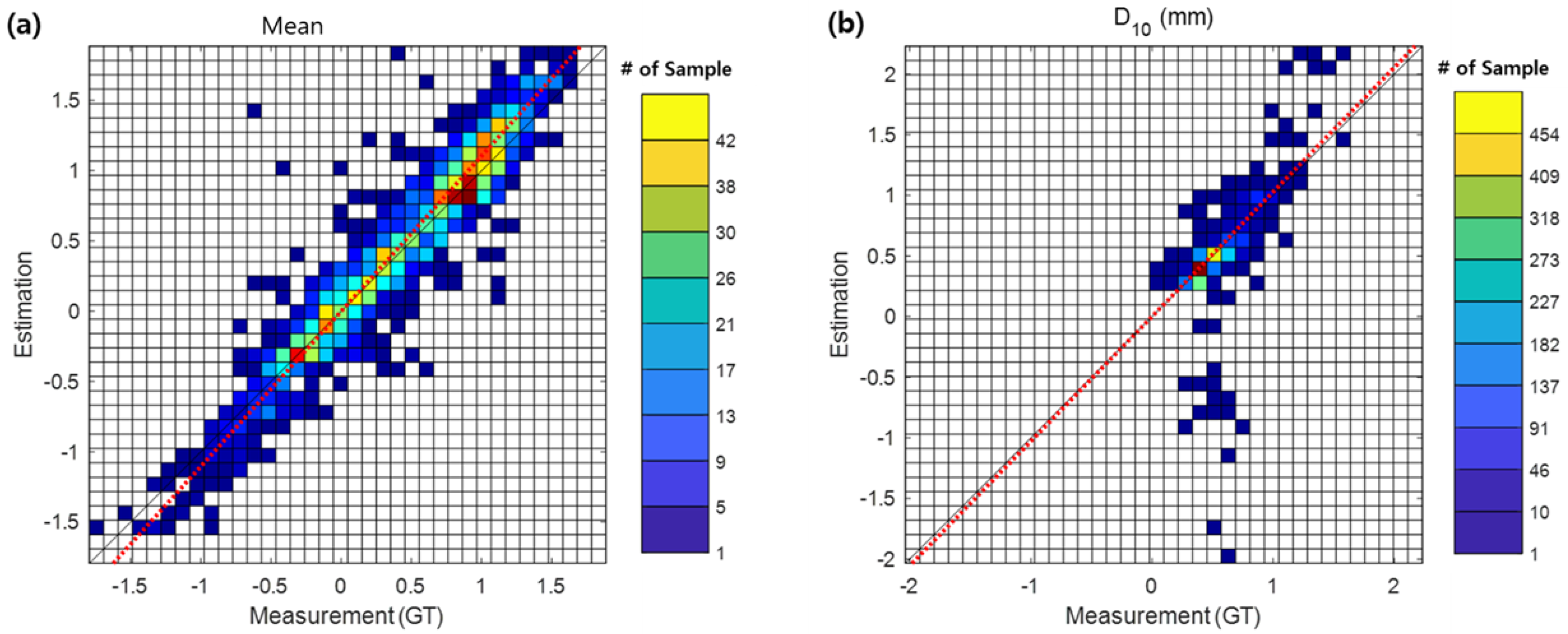
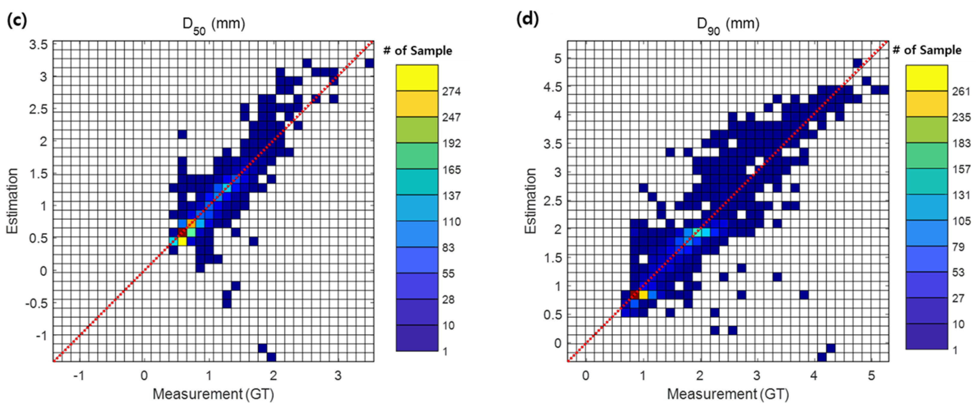
In particular, Figure 5 shows a scatter plot comparing the ground-truth measurements with the estimated values of mean grain size, $D_{10}$, $D_{50}$, and $D_{90}$ from the proposed model with data augmentation for the entire test dataset. The symmetric slopes $\rho$, indicated by the red dotted lines in Figure 5, are 1.105, 1.028, 1.006, and 1.007 for mean grain size, $D_{10}$, $D_{50}$, and $D_{90}$, respectively. For the mean diameter, the estimated results show very good agreement with the measurements overall, with only a small number of samples showing discrepancies.

Table 3. Error statistics of RMSE, bias, and Pearson correlation coefficient (CC) for the model estimates and ground-truth measurements of the grain diameter (mm), $D_{10}$ (mm), $D_{50}$ (mm), and $D_{90}$ (mm) for the proposed model.

Metric	Mean	${\mathit{D}}_{10}$ (mm)	${\mathit{D}}_{50}$ (mm)	${\mathit{D}}_{90}$ (mm)
RMSE (mm)	0.21	0.19	0.22	0.36
Bias (mm)	0.04	−0.03	−0.02	−0.02
CC	0.95	0.72	0.88	0.91

shows a very high CC of 0.95. For $D_{10}$, overestimation occurs for samples above 1.2 mm, and underestimation occurs for samples below 0.8 mm. However, for most samples with values between 0.3 and 1.5 mm, the measurements and estimated results are in good agreement, with a CC of 0.88. For $D_{50}$, some samples between 1.3 and 2 mm are underestimated, while some samples above 2.5 mm are overestimated. Overall, the agreement is good, with a CC of 0.88. The results for $D_{90}$ show a tendency to slightly overestimate overall, but they are in good agreement, with an overall CC of 0.91. However, some samples are underestimated in the range of 2.0–4.2 mm.

Table 3 shows error statistics for RMSE, bias, and correlation coefficient for mean grain size, $D_{10}$, $D_{50}$, and $D_{90}$. For the four estimation variables, the bias ranges from 0.02 to 0.04 mm, indicating a very small difference between the measurements and estimated values. RMSE values range from 0.19 to 0.36 mm. In terms of the CC, the mean diameter and $D_{90}$ exhibit a high correlation of 91–95%, while $D_{50}$ shows a correlation of 88%. $D_{10}$ shows a somewhat lower correlation of 72% but still demonstrates a reasonable relationship.

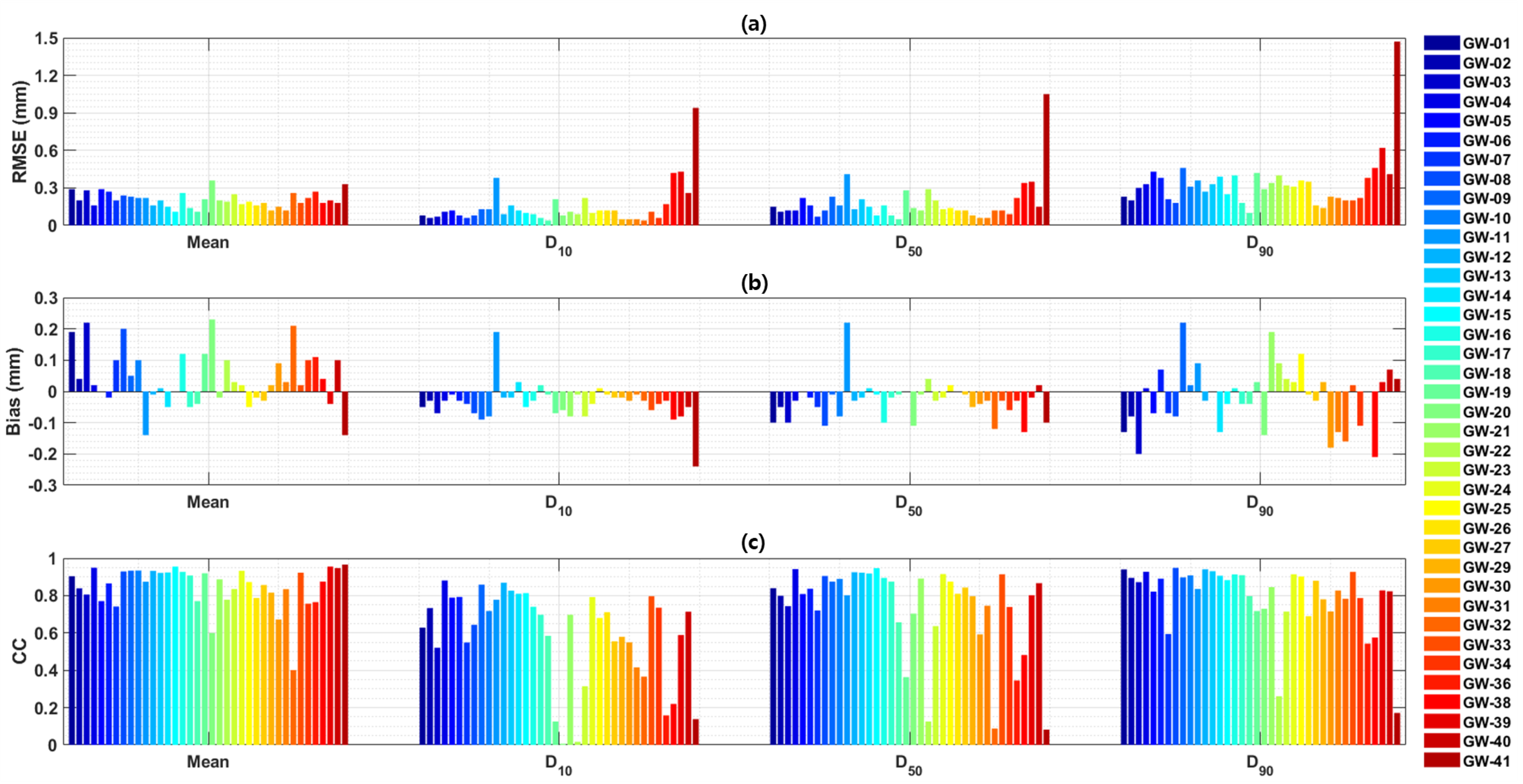
Figure 6 shows the RMSE, bias, and CC for mean grain size, $D_{10}$, $D_{50}$, and $D_{90}$ for each littoral system. Overall, as the particle size increases ($D_{10}$$\to$$D_{90}$), the estimation RMSE tends to increase, as can be seen in Figure 6a. In Table 1, the littoral system with the largest values for $D_{10}$, $D_{50}$, and $D_{90}$ is GW11, with values of 1.15 mm, 2.06 mm, and 3.73 mm, respectively, which shows the lowest performance in terms of RMSE, bias, and CC, as shown in Figure 6. In particular, GW41 has the highest RMSE for $D_{10}$, $D_{50}$, and $D_{90}$, indicating the lowest distribution estimation performance. The $D_{10}$, $D_{50}$, and $D_{90}$ values for GW41 are 0.14 mm, 0.98 mm, and 2.56 mm, respectively. Although the values for $D_{50}$ and $D_{90}$ fall within a larger range compared to the surrounding littoral systems (see Table 1), the reason for the high RMSE and low CC, despite not having the largest values, is likely due to the high variance in the distributed particle sizes, which is 0.90. Additionally, as shown in the bar graph for CC in Figure 6c, the CC values for $D_{10}$ are very low for GW20 and GW22, with values of 0.01 and 0.02, respectively. This is likely due to samples that are significantly overestimated or underestimated, as seen in Figure 5b. Moreover, the mean grain diameters for these two systems are 1.33 and 1.16, which are higher than the average values (see Table 1). The CC for $D_{50}$ is also the lowest for GW30 and GW40, with values of 0.09 and 0.08, respectively. This is likely due to the significant underestimation observed in Figure 5c. Additionally, as seen in Table 1, the number of samples for GW40 is smaller compared to other littoral systems, which may also have an impact on the results. For $D_{90}$, the CC values for GW22 and GW41 are also low, at 0.26 and 0.17, respectively. This is considered to be due to the influence of underestimating samples, as seen in Figure 5d. In particular, by examining the sample images for each system in Figure 3, it can be visually observed that in GW26, GW30, and GW40, some particles exhibit outlier-like distributions within a single image. While this is not a characteristic of the entire test data and does not significantly affect the overall average performance, it is expected to cause some performance degradation in individual test results. However, for GW11 and GW41, this is not an anomaly but rather a clear indication of high variation in the grain size distribution of the sand in those regions, which can also be visually checked. For these two littoral systems, the performance of distribution estimation for grain size is somewhat lower compared to other littoral systems.

7. Conclusions

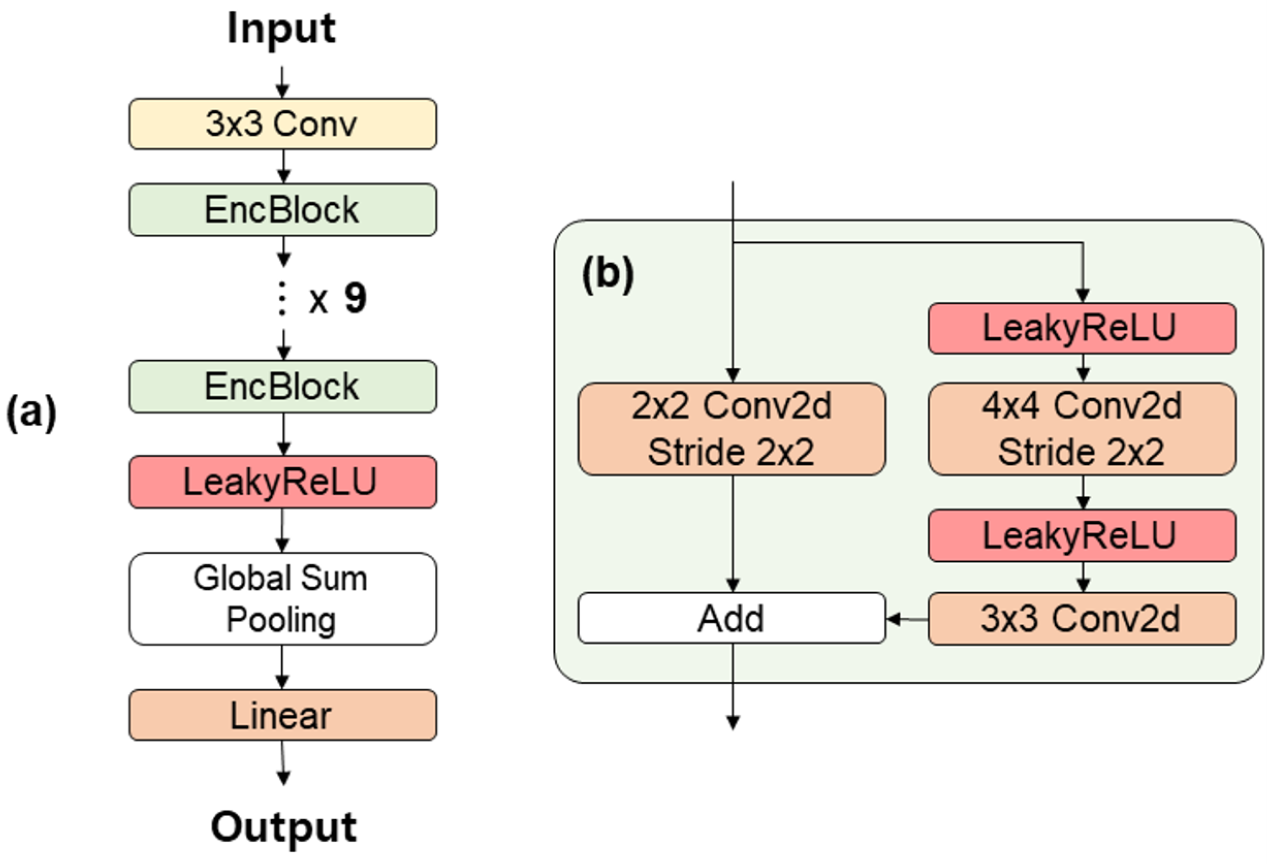
In this study, we propose a 2D CNN-based spatial encoder network for estimating grain size distribution from optical images of sediments using spatial feature representation learning and data augmentation. The proposed model was applied to 41 littoral systems along the east coast of Gangwon Province, Korea. Grain size distribution was measured through sieve analysis for sediments collected from these 41 littoral systems between 2010 to 2024. A total of 6337 optical images, each mapped to corresponding measurements, were acquired and used to develop the data-driven model. In total, seven variables are used to estimate the size distribution: mean grain size, standard deviation, skewness, kurtosis, $D_{10}$, $D_{50}$, and $D_{90}$. In particular, when estimating grain size from sediment images, sufficient network capacity was achieved by deeply stacking multiple EncBlocks, enabling the model to understand and learn the spatial feature representation of the optical image. Additionally, to enhance the robustness and reliability of the model, data augmentation was applied using geometric transformations, including horizontal and vertical flipping methods for the training data.

For the grain size distribution estimated through the proposed model, we achieved improved performance for all output variables compared to the previous DL-based method. This improvement is attributed to the model’s ability to learn the spatial feature representation of images through the proposed network’s sufficient capacity. Additionally, we quantitatively evaluated the improved performance through data augmentation. In particular, the mean diameter for grain size estimated from sediment images demonstrated very high accuracy with a CC of 95%. For $D_{10}$, $D_{50}$, and $D_{90}$, we also observed good correlations of 97%, 88%, and 91%, respectively.

Overall, the prediction performance is good; however, the model tends to show slightly deteriorated performance as the diversity of the grain size distribution increases or the particle size becomes larger. Some samples that are overestimated or underestimated contributed to the performance degradation. In cases where the number of samples per littoral system was relatively small, this also had some impact on the performance evaluation, but with the construction of a large number of data samples over a long-term period, it did not pose a significant issue when considering the overall average performance.

Understanding sediment transport is crucial across various disciplines because it plays a key role in geomorphology, hydrology and fluvial engineering, ecology, and environmental science, as well as in addressing climate change. In particular, understanding sediment transport in coastal management is essential for predicting coastal erosion, designing coastal structures and assessing their effectiveness, maintaining ports and shipping lanes, conserving coastal ecosystems, preserving beaches and the tourism industry, responding to climate change, and preventing disasters. However, collecting sediment samples and measuring grain size in the field can be challenging, and there are limitations in both the time and spatial resolution of measurement data. However, if grain size distribution can be accurately estimated using sediment images as in the proposed method, it would provide a considerable advancement over traditional, complex, and labor-intensive measurement techniques. The sediment images used in this study primarily consist of sand-dominated samples and can serve as a remote sensing-based observation method, offering sufficient accuracy for sites with similar sediment compositions to those found along the east coast of Gangwon Province, Korea. To increase the applicability of this approach in the future, data from a wider variety of sediments will be collected, and additional training will be performed. In addition to the characteristics of the grain size distribution, colorimetric information will also be estimated from the images. This is expected to be useful for applications such as determining sediment for sand nourishment in coastal management.