Article

Generation and Evolution of Cnoidal Waves in a Two-Dimensional Numerical Viscous Wave Flume

1
Department of Environmental Engineering and Science, Chia Nan University, Tainan City 71710, Taiwan
2
Department of Hydraulic and Ocean Engineering, National Cheng Kung University, Tainan City 70101, Taiwan
3
Coastal Ocean Monitoring Center, National Cheng Kung University, Tainan City 70101, Taiwan
*
Author to whom correspondence should be addressed.
J. Mar. Sci. Eng. 2025, 13(6), 1102; https://doi.org/10.3390/jmse13061102
Submission received: 17 April 2025 / Revised: 28 May 2025 / Accepted: 29 May 2025 / Published: 30 May 2025
(This article belongs to the Section Ocean Engineering)

Abstract

The generation and propagation of water waves in a numerical wave flume with Ursell numbers (Ur) ranging from 0.67 to 43.81 were investigated using the wave generation theory of Goring and Raichlen and a two-dimensional numerical viscous wave flume model. The unsteady Navier–Stokes equations, along with nonlinear free surface boundary conditions and upstream boundary conditions at the wavemaker, were solved to build the numerical wave flume. The generated waves included small-amplitude, finite-amplitude, cnoidal, and solitary waves. For computational efficiency, the Jacobi elliptic function representing the surface elevation of a cnoidal wave was expressed as a Fourier series expansion. The accuracy of the generated waveforms and associated flow fields was validated through comparison with theoretical solutions. For U r < 26.32 , small-amplitude waves generated using Goring and Raichlen’s wave generation theory matched those obtained from linear wave theory, while finite-amplitude waves matched those obtained using Madsen’s wave generation theory. For U r > 26.32 , nonlinear wave generated using Goring and Raichlen’s theory remained permanent, whereas that generated using Madsen’s theory did not. The evolution of a cnoidal wave train with U r = 43.81 was examined, and it was found that, after an extended propagation period, the leading waves in the wave train evolved into a series of solitary waves, with the tallest wave positioned at the front.

1. Introduction

Two-dimensional (2D) wave flumes have been widely used to study the interaction of waves and structures and to perform physical model tests for various applications in ocean and coastal engineering. There are currently two primary types of wave generators utilized in the laboratory: piston-type and flap-type wavemakers.
Piston-type wavemakers are commonly employed to generate shallow water waves, while flap-type wavemakers are better suited for producing deep water waves [1]. Havelock [2] applied linear wave theory to derive theoretical solutions for both piston-type and flap-type wavemakers. The accuracy of these linear theory solutions was experimentally confirmed by Ursell et al. [3] for piston-type wavemakers and by Hudspeth et al. [4] for flap-type wavemakers.
As the amplitude of generated waves increases, the waveforms predicted by linear wave generation theory change depending on the measurement location, resulting in non-permanent wave shapes. This phenomenon was first observed by Goda [5], and Madsen [6] provided an analytical explanation for this phenomenon. Madsen [6] also derived the motion function of a piston-type wavemaker for generating second-order Stokes waves. However, Buhr Hansen and Svendsen [7] noted that if the Ursell number (defined as U r = H L 2 / h o 3 , where H is the wave height, L is the wavelength, and h o is the still water depth; Ur represents the ratio of wave nonlinearity strength to dispersion strength) exceeds 30, the waves generated using Madsen’s wave generation theory are not permanent, suggesting a shift to the generation of cnoidal waves.
In numerous experiments on wave flumes, the wave generation theory introduced by Goring and Raichlen [8] has been employed to produce solitary waves and cnoidal waves. Goring and Raichlen [8] investigated the suitability of their theory for generating waves across the Ursell number range 10–1230. They observed that the waves with higher Ursell numbers generated using their theory closely matched the results obtained from the Korteweg–de Vries (KdV) equation.
As previously mentioned, analytical solutions for piston- and flap-type wavemakers were derived by Havelock [2]. These solutions were based on linear wave theory and potential flow theory, which assumes an inviscid fluid and irrotational flow. Ohyama and Nadaoka [9], as well as Grilli and Horillo [10], applied potential flow theory to develop computational wave flumes capable of simulating nonlinear and random wave patterns. They also proposed a numerical wave-absorption filter to simulate open boundary conditions. Similarly, Guyenne and Nicholls [11] developed a numerical method, also grounded in potential flow theory, for simulating nonlinear surface water waves over both static and moving bottom boundaries. They demonstrated the effectiveness of their approach through a series of two-dimensional simulations, including linear wave shoaling, Bragg reflection over sinusoidally varying topography, and tsunami generation due to impulsive bottom displacement.
Although the wave generation problem has been addressed by previous researchers [2,3,4,6,7,8,9,10,11], their solutions were derived based on potential flow theory, which assumes that the flow is inviscid and irrotational. Lamb [12] noted that viscosity has only a relatively minor effect on free oscillatory waves in deep water. However, viscosity is crucial for a comprehensive understanding of the real viscous flow generated by the interaction between water waves and offshore structures. For example, when waves propagate over a submerged breakwater, vortex generation near the structure and the associated viscous drag are critical factors influencing its stability [13,14]. These phenomena cannot be captured by potential flow theory. Consequently, a numerical wave flume equipped with a wavemaker that incorporates fluid viscosity is necessary to simulate the vortex dynamics induced by wave–structure interactions.
Huang et al. [15] developed a 2D numerical viscous wave flume produced with a piston-type wavemaker. They solved the Navier–Stokes equations with nonlinear free surface boundary conditions to simulate nonlinear viscous wavefields. Following the methodology of Huang et al. [15], Dong and Huang [16] investigated the generation and propagation of various wave types—including small-amplitude, finite-amplitude, and solitary waves—within a wave flume model. Dong and Huang [16] applied linear wave generation theory to produce small-amplitude waves, while using Madsen’s [6] wave generation theory to generate permanent second-order Stokes waves with simulated Ursell numbers below 25.9. Additionally, the wave generation theory of Goring and Raichlen [8] was employed to generate solitary waves. The numerical results for the waveforms and associated boundary-layer flows induced by the small-amplitude, finite-amplitude, and solitary waves were validated through comparison with corresponding theoretical solutions. Dong and Huang [16] not only examined whether the generated waves maintained a permanent form during propagation but also studied the evolution of these waves after extended periods of propagation in a numerical wave flume.
Solitary waves and cnoidal waves are commonly used to model tsunamis [17]. Cnoidal waves are also believed to be appropriate for modeling important aspects of the coastal effects of finite-amplitude long waves that propagate from deep to shallow water. Cnoidal waves are nonlinear, exact solutions of the KdV equation, expressed using the Jacobi elliptic function (cn). In the low-amplitude limit, cnoidal waves resemble sinusoidal profiles, while high-amplitude cnoidal waves develop narrow peaks, closely approximating the sech² shape of solitary waves. As such, cnoidal waves serve as a general framework for representing both linear and nonlinear periodic waveforms.
To date, the generation and evolution of cnoidal waves have been relatively less studied, especially in comparison to solitary waves. Lin and Liu [18] demonstrate that various waves, including cnoidal waves, can be generated by employing internal source functions in a numerical wave flume method based on solving the Navier–Stokes equations. Liu et al. [19] developed a numerical wave flume method for generating solitary and cnoidal waves in shallow water by using various theories, including the Green–Naghdi equations [20], the Keulegan and Patterson equations [21], and the KdV equations [22,23]. In their numerical analysis, they employed the open-source computational fluid dynamics package OpenFOAM [24] and solved the Navier–Stokes equations. Svendsen and Brink-Kjær [25] developed a method for calculating changes in cnoidal waves’ height and wavelength due to the shoaling of these waves. Synolakis and Deb [26] developed an approximate theory to estimate the maximum run-up of nonbreaking cnoidal waves on plane beaches. Their study demonstrates that, for waves of the same height and wavelength, cnoidal waves generate a significantly greater maximum run-up compared to monochromatic waves. This theory has been supported by laboratory experiments. Additionally, Lee and Tang [27] carried out a numerical study on the propagation of cnoidal waves over a wavy bed.
Another issue related to the propagation of wave trains in a channel is whether the wave train remains stable after traveling for a long period. A flow becomes unstable when energy transfers from the primary flow to disturbances at a rate faster than the energy dissipates due to viscosity. Such disturbances can occur if the wave paddle’s motion experiences slight modulation. Benjamin and Feir [28] were the first to theoretically investigate the instability of wave trains in deep water, while Su et al. [29] conducted a similar experimental study in a 3.7 × 3.7 × 137.2   m towing tank. Benjamin [30] and Whitham [31] showed that Stokes wave trains in water of finite depth become unstable when the fundamental wavenumber k satisfies, k h o > 1.363. In contrast, Benjamin [32], along with Pego and Weinstein [33], proved that, unlike nonlinear periodic waves, solitary waves propagate stably in a channel. Further research by Angulo Pava et al. [34], Bottman and Deconinck [35], and Deconinck and Kapitula [36] have shown that cnoidal waves are stable under small periodic perturbations.
Research on wave generation in numerical wave flumes has rarely explored the evolution of waves after prolonged propagation. This area of study is particularly intriguing, as it offers valuable insights into wave behavior over long distances. Such studies are often impractical in a physical wave flume due to its limited length. Moreover, this research could serve as a test of a numerical wave flume’s ability to generate and propagate waves over extended periods and long distances from the wavemaker. Dong and Huang [16] examined the evolution of wave sequences over long distances using a numerical wave flume that accounts for fluid viscosity; however, their study was limited to waves in finite water depths, with a Ursell number ranging from 0.67 to 25.9.
The objective of this study is to develop a 2D numerical viscous wave flume capable of generating water waves ranging from small to large amplitude using a unified wavemaking theory. The accuracy and robustness of the flume are examined. The accuracy of the model is demonstrated by verifying the precision of the generated waveforms and the flow velocity profiles within the wave-induced bottom boundary layer. The robustness of the flume is evaluated by studying the evolution of the waves after prolonged propagation within the flume.
The present study builds upon Dong and Huang’s [16] work by increasing the maximum Ursell number from 25.9 to 43.81. Consequently, the waves studied now include cnoidal waves, in addition to small-amplitude, large-amplitude, and solitary waves. According to Buhr Hansen and Svendsen [7], Madsen’s wave generation theory is valid only for waves with U r < 30 . Unlike Dong and Huang [16], who used different wave generation theories to produce small-amplitude, finite-amplitude, and solitary waves, this study applied the wave generation theory of Goring and Raichlen [8] to generate all the waves studied, with Ursell numbers ranging from 0.67 to 43.81.
The waves studied in this research are classified as intermediate-deep-water waves with k h o values less than 1.363. According to Benjamin [30] and Whitham [31], Stokes wave trains within this range are stable. Furthermore, as previously mentioned, Angulo Pava et al. [34], Bottman and Deconinck [35], and Deconinck and Kapitula [36] demonstrated that cnoidal waves remain stable under small perturbations. Hence, in theory, all nonlinear waves examined in this study, including Stokes waves, cnoidal waves, and solitary waves, are stable. However, the evolution of leading waves in a wave train has rarely been studied. Investigating their development provides valuable insights into the dynamics and behavior of waves propagating from a distant source under varying conditions. While Dong and Huang [16] explored the evolution of leading waves in wave trains with Ursell numbers ranging from 0.67 to 25.9, the behavior of leading waves in a cnoidal wave train remains unknown and requires further investigation.
Based on the discussion of the relevant literature, the key contributions of this study are as follows: This work develops a 2D numerical viscous wave flume capable of generating small-amplitude, finite-amplitude, cnoidal, and solitary waves using a unified wavemaking theory. After verifying the accuracy of the flume, the study investigates the evolution of leading waves in a cnoidal wave train with U r = 43.81 . The findings reveal that, after prolonged propagation, the leading waves in the wave train transform into a series of solitary waves—an observation not previously reported in the existing literature.
The rest of this paper is organized as follows. Section 2 provides a brief overview of the numerical methods employed to solve the governing equations and boundary conditions. Section 3 discusses the theories used to generate small-amplitude, finite-amplitude, cnoidal, and solitary waves. Next, the accuracy of the generated waves in the flume is evaluated, focusing on the waveform and flow velocity profile, including that in the bottom boundary layer. Finally, the evolution of the leading waves in a cnoidal wave train after extended propagation is analyzed.

2. Numerical Methods

The computational models proposed by Huang et al. [15] and adapted by Dong and Huang [16] were employed to study the behavior of cnoidal waves in a 2D viscous wave simulation. Figure 1 shows a schematic of a two-dimensional numerical wave flume with a flat bottom. At x = 0, a piston-type wavemaker produces the incoming waves.
For details about the governing equations, and the boundary conditions at the free surface, the bottom of the flume, and downstream used in the numerical scheme, refer to Dong and Huang [16]. The main concepts underlying this method are briefly described as follows.
The Finite-Analytic method developed by Chen and Chen [37] was applied to discretize the dimensionless Navier–Stokes equations for viscous, incompressible flow in Cartesian coordinates. To resolve the coupled pressure and velocity fields, the SIMPLER algorithm by Patankar [38] was employed, utilizing a staggered grid arrangement to prevent pressure–velocity decoupling.
To ensure numerical stability and convergence, the time step in this study was chosen to keep the Courant number below 1.0. A non-dimensional time step of 0.004 was used in the simulations. For the case with U r = 43.81 (corresponding to a water depth of 0.4 m, wave height of 8.0 cm, and wave period of 3 s), this translates to a dimensional time step of approximately 0.0035 s. As a result, each wave period is divided into about 850 time steps, providing sufficient temporal resolution. The free surface was reconstructed using the SUMMAC (Stanford University Modified MAC) method [39]. Its position was primarily tracked using a Lagrangian approach, wherein the motion of marker points assigned to the free surface was explicitly followed.
In regions requiring higher computational accuracy—particularly within boundary layers—a finer mesh was applied to improve resolution. Uniform grid spacing was used in the horizontal and vertical directions, Δ x / h o = 0.25 and Δ   y / h o   = 0.05 , except near the flume’s bottom boundary, where adjustments were made to account for increased flow complexity. To accurately capture boundary layer flows induced by waves, the vertical grid size within a distance of 5δ from the bottom (0 < y < 5δ) was set to Δy = 5δ/20, where δ = 2 ν / ω is the characteristic boundary layer thickness, ν is the kinematic viscosity of the fluid, and ω is the angular frequency of the waves. In the subsequent region (5δ < y < 10δ), the vertical grid size was Δy = 5δ/10. Additionally, the horizontal velocity at the outer edge of the boundary layer was matched with the bottom horizontal velocity derived from the potential flow theory. Grid refinement was applied in both the x- and y-directions, as well as near the free surface, to ensure that simulation results were independent of mesh resolution.
To produce the desired incident waves, it was necessary to determine the lateral boundary condition at the wavemaker. This topic is covered in the next section.

3. Wavemaker Theories

3.1. Linear and Madsen’s Theories

Dong and Huang [16] provided a detailed discussion on using a piston-type wavemaker to generate small-amplitude, finite-amplitude, and solitary waves in a 2D numerical wave flume. For completeness, the related wavemaking theories are briefly described in this section.
For producing small-amplitude waves with a surface elevation of η = a sin ( k x ω t ) , where a is the wave amplitude; k is the wavenumber and ω is the angular frequency, the displacement of the wavemaker can be determined using linear wavemaker theory [1] as follows:
ξ ( t ) = ξ o cos ω t
with
ξ o = a n 1 tanh k h o ,   n 1 = 1 2 ( 1 + 2 k h o sinh 2 k h o )
The corresponding horizontal velocity within the near-bed boundary layer, induced by wave action, is given by the following:
u = g a k ω cosh k h o [ cosh k y e y cos ( ψ + y ) ]
where y = y / δ , δ = 2 ν / ω , and ψ = k x ω   t .
Madsen [6] found that if the motion of the wavemaker, described by Equation (1), is used to generate finite-amplitude waves, the waves in the flume are affected by a significant free second harmonic, which greatly disturbs the wave profiles. As a result, the generated waves do not maintain a permanent form. To suppress second-order free waves generated by a sinusoidal paddle motion, Madsen [6] proposed a specific wavemaker displacement profile as follows:
ξ = ξ o [ cos ω t + a 2 h o n 1 ( 3 4 sinh 2 k h o n 1 2 ) sin 2 ω t ]
This wave generation method produces Stokes second-order waves, which maintain a stable shape over time. Mizuguchi [40] derived the horizontal velocity distribution within the bottom boundary layer under these wave conditions.
Madsen’s wave generation theory can produce Stokes second-order waves without contamination from second-order free waves, allowing the waves to propagate in a permanent form. However, for large waves, the second-order harmonic of the Stokes waves may introduce anomalous bumps in the wave troughs. Dean and Dalrymple ([1], Section 11.2.4) indicated that for Stokes waves in shallow water with k a ( k h ) 3 / 3 , which corresponds to U r = λ 2 H h 3 8 π 2 3 = 26.32 , these anomalous bumps do not appear. Therefore, when applying Madsen’s wave generation theory to generate Stokes second-order waves in shallow water with a periodic waveform, it should be limited to cases where the Ursell number is less than 8 π 2 / 3 (or 26.32). The threshold value of U r = 30 suggested by Buhr Hansen and Svendsen [7] is only an approximation. In this study, nonlinear waves generated in finite water depth with U r > 26.32 are referred to as cnoidal waves.

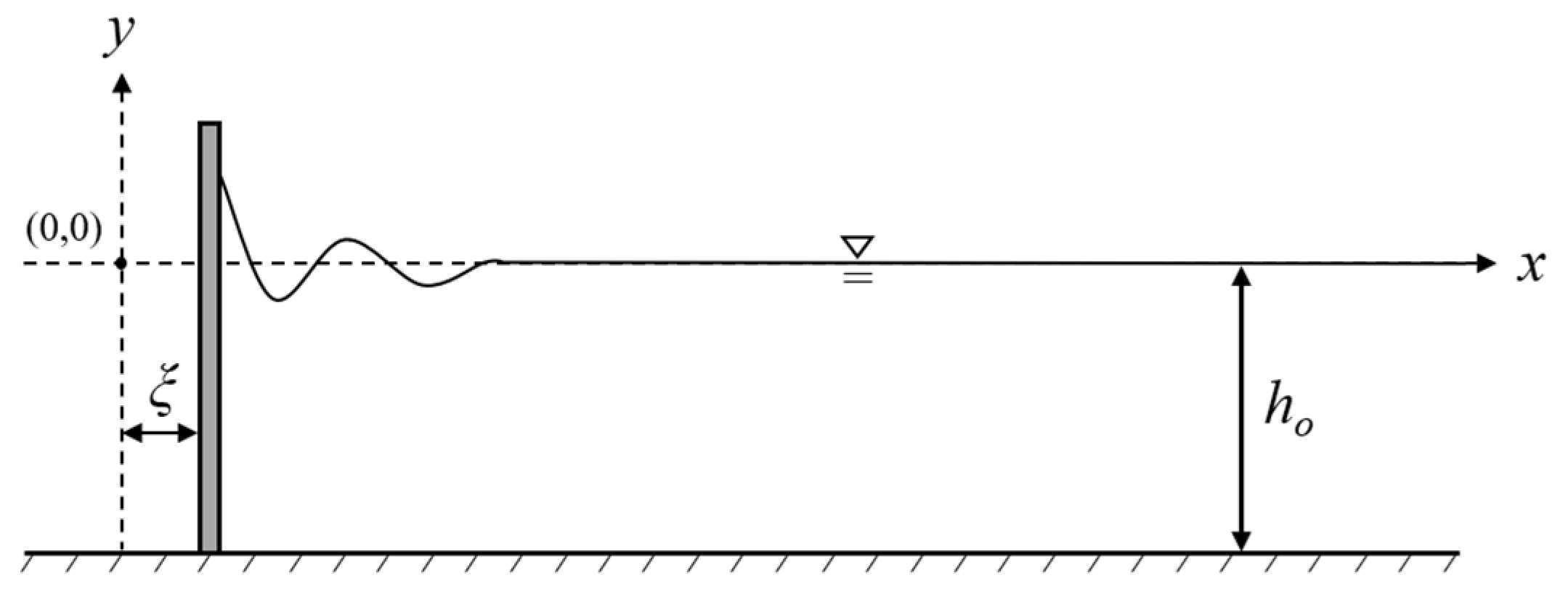
3.2. Goring and Raichlen’s Theory

Regarding the generation of nonlinear shallow-water waves of permanent shape by using a piston-type wavemaker, on the basis of the continuity equation, Goring and Raichlen [8] proposed the following equation relating the velocity of the wavemaking plate to waves with water elevation of η ( x , t ) (refer to Figure 1):
d ξ ( t ) d t = u m ( t ) = c η ( x , t ) h o + η ( x , t )
where t is time, x is the coordinate, ξ is the displacement of the plate, u m ( t ) is the velocity of the wavemaking plate, h o is the still water depth, and c is the wave celerity. Thus, when the water elevation of the desired wave is given, Equation (5) can be used to determine the velocity of the wavemaking plate.
Equation (5) was employed by Dong and Huang [16] to generate a solitary wave. The surface elevation of a solitary wave can be expressed as
η = H i sec h 2 [ K ( x c t ) ] ,   K = 3 H i / 4 h o 3
Substituting this expression for η into Equation (5) gives a differential equation, which can be solved to obtain the following:
ξ ( t ) = H i K h o tanh K ( c t x )
Huang and Dong [14] examined the near-bed flow profile induced by a solitary wave and demonstrated that the resulting horizontal velocity satisfies second-order boundary matching conditions.

4. Results and Discussion
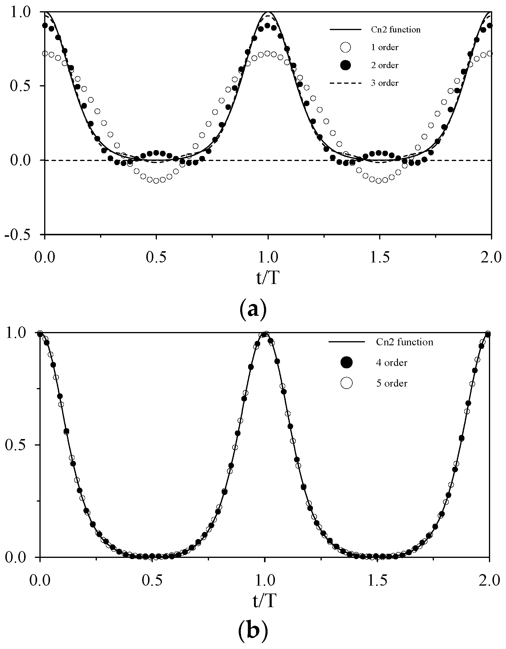
4.1. Cnoidal Waves

The surface elevation η ( x , t ) as a function of horizontal position x and time t for a cnoidal wave is expressed as follows [41]:
η ( x , t ) = η 2 + H c n 2 [ 2 K ( m ) L ( x c t ) ]
η 2 = H m 2 [ 1 m 2 E ( m ) K ( m ) ]
where η 2 is the trough elevation, H is the wave height, L is the wavelength, c is the wave speed, cn is one of the Jacobi elliptic functions, and K ( m ) and E ( m ) are the complete elliptic integrals of the first and second kind, respectively; m is the modulus of a Jacobi elliptic function, with 0 < m < 1.
The wavelength and wave speed of the cnoidal wave are
L = 4 K ( m ) h o m 2 h o 3 H
and
c = g h o [ 1 + H h o 1 m 2 ( 2 m 2 3 E ( m ) K ( m ) ) ] 1 / 2
The wave period T can be obtained by dividing L by c:
T g h o = 16 h o 3 H K ( m ) m / [ 1 + H h o 1 m 2 ( 2 m 2 3 E ( m ) K ( m ) ) ] 1 / 2
In the limiting case, when m 2 1 , E ( m ) = 1 , K ( m ) , and c n 2 ( ) = sec h 2 ( ) , Equation (8) becomes
η ( x , t ) = H sec h 2 [ 3 H 4 h o 3 ( x c t ) ]
The surface elevation in Equation (13) is that of a solitary wave. Similarly, when m 2 0 , E ( m ) = π 2 , K ( m ) = π 2 , and c n 2 ( ) = cos 2 ( ) , Equation (8) becomes
η ( x , t ) = η 2 + H cos 2 [ π L ( x c t ) ]
Letting η 2 = H 2 , the above equation can be rewritten as follows:
η ( x , t ) = H 2 cos [ k ( x c t ) ]
The surface elevation in Equation (14) is that of a linear wave with a sinusoidal profile.
In this study, a cnoidal wave was specified by its wave height, wave period, and water depth. Solving Equation (12) through iteration provided the values for the variables m , K ( m ) , and E ( m ) under the given conditions. Substituting these values back into Equations (10) and (11) enabled the calculation of the wavelength and phase speed of the cnoidal wave. In this way, the water surface elevation of the cnoidal wave and the corresponding velocity function of the wavemaking plate at any time could be determined from Equations (8) and (5), respectively.
The Jacobi elliptic functions are periodic and can be expressed as a Fourier series expansion. According to Byrd and Friedman [42], Isobe [43], Kiper [44], and Tanaka et al. [45], the Fourier series expansion for c n 2 can be expressed as follows:
c n 2 [ 2 K ( m ) L ( x c t ) ] = n = 0 A n cos [ 2 n π ( x / L t / T ) ]
The coefficient A n is as follows:
A n = E ( m ) K ( m ) m 2 K ( m ) m 2 , n = 0 2 π 2 m 2 K 2 ( m ) ( n q n 1 q 2 n ) ,   n 1
where m is the complementary modulus of the Jacobi elliptic functions and equals 1 m 2 , and q = exp [ π K ( m ) / K ( m ) ] . From Equations (8) and (15), the surface elevation of a cnoidal wave can be expressed as
η ( x , t ) = η 2 + H n = 1 N A n cos [ 2 n π ( x / L t / T ) ]
For computational convenience, the numerical wave generation model used in this study employed Equation (17) to calculate the water level of the cnoidal wave. Regarding the selection of the number of terms N in the Fourier series to achieve the desired accuracy, Tanaka et al. [45] demonstrated that setting N to 5 results in a relative error between the synthesized function and the original function of less than 1%. Therefore, N = 5 was employed as the basis for the calculations.
To examine the disparities between the approximations synthesized using first- to fifth-order Fourier series and the original function ( c n 2 ), Figure 2 compares the theoretical waveform of a cnoidal wave with zero trough elevation and h o = 0.4 m, H i = 8.0 cm, T = 3.0 s, and U r = 43.81 with the approximations synthesized through first- to fifth-order Fourier series. The figure clearly shows that, under the given wave conditions, the accuracy with which the fourth- and fifth-order Fourier series fit the square of the Jacobi elliptic cosine function is satisfactory.

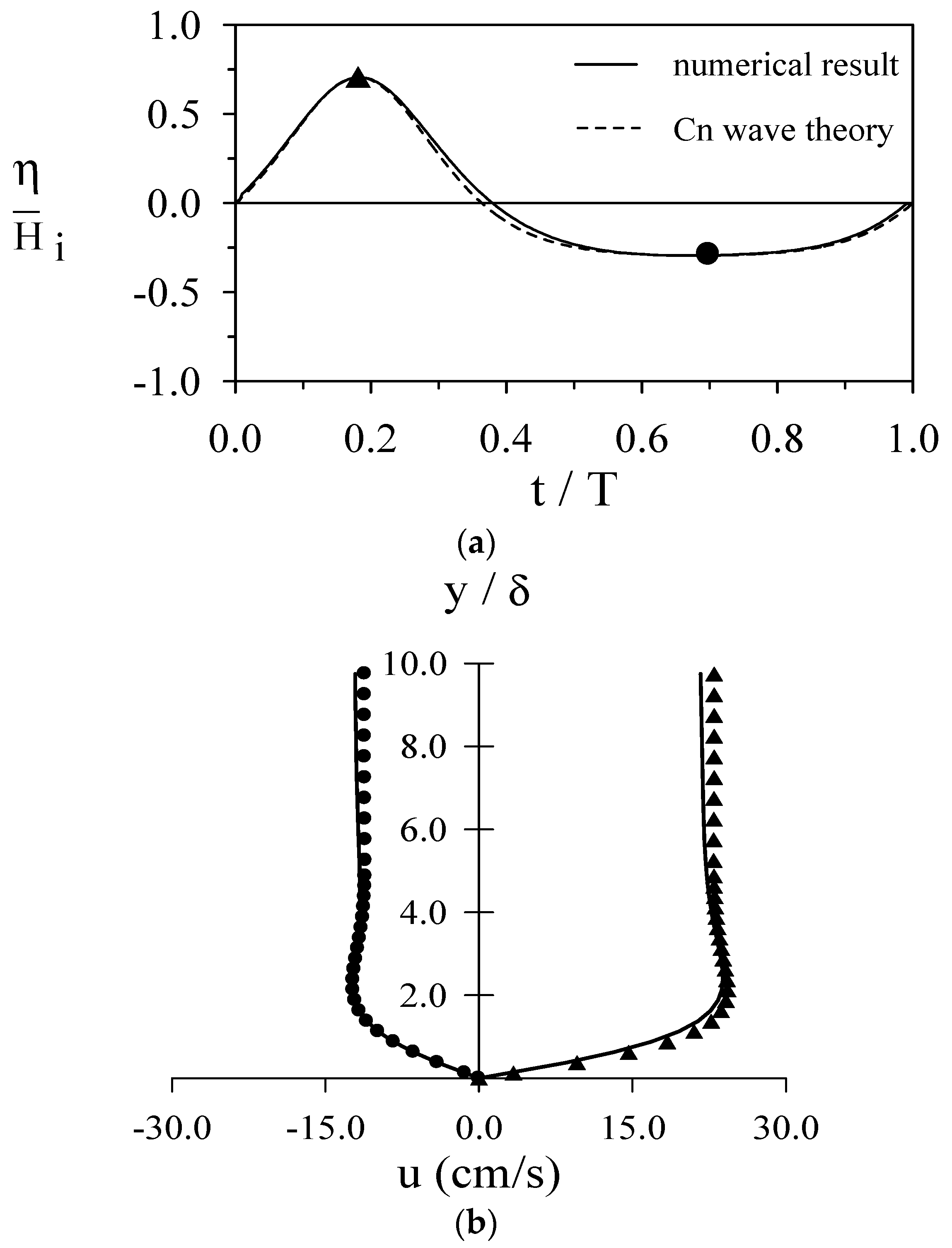
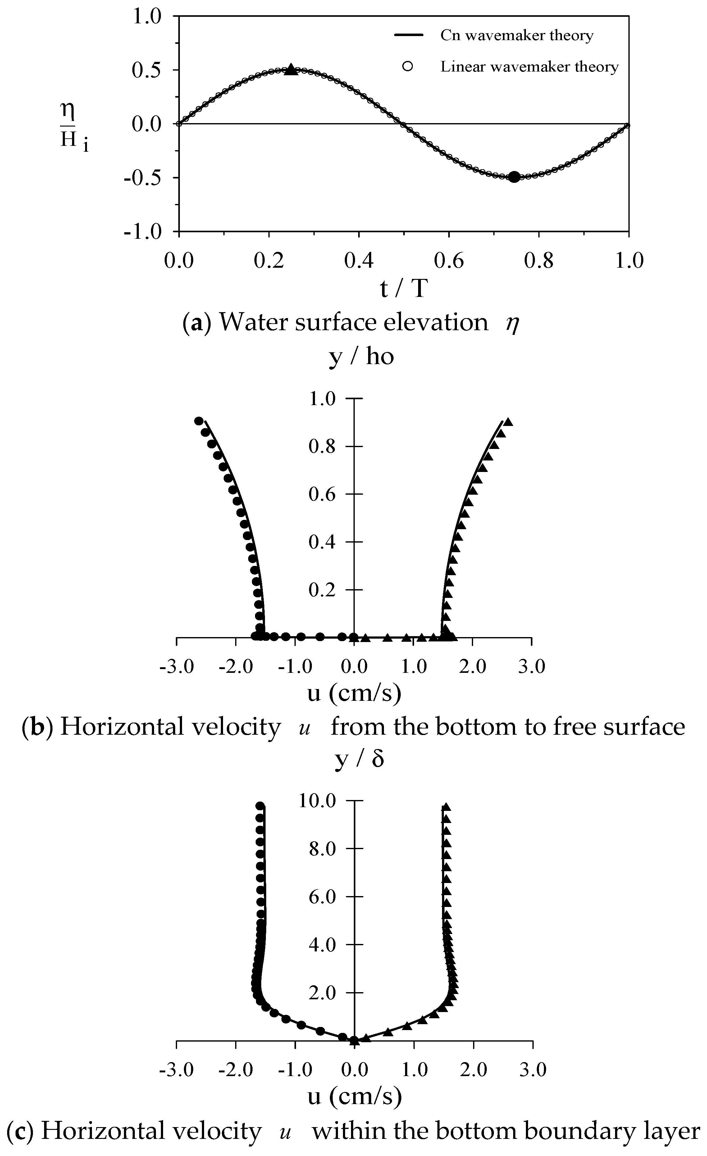
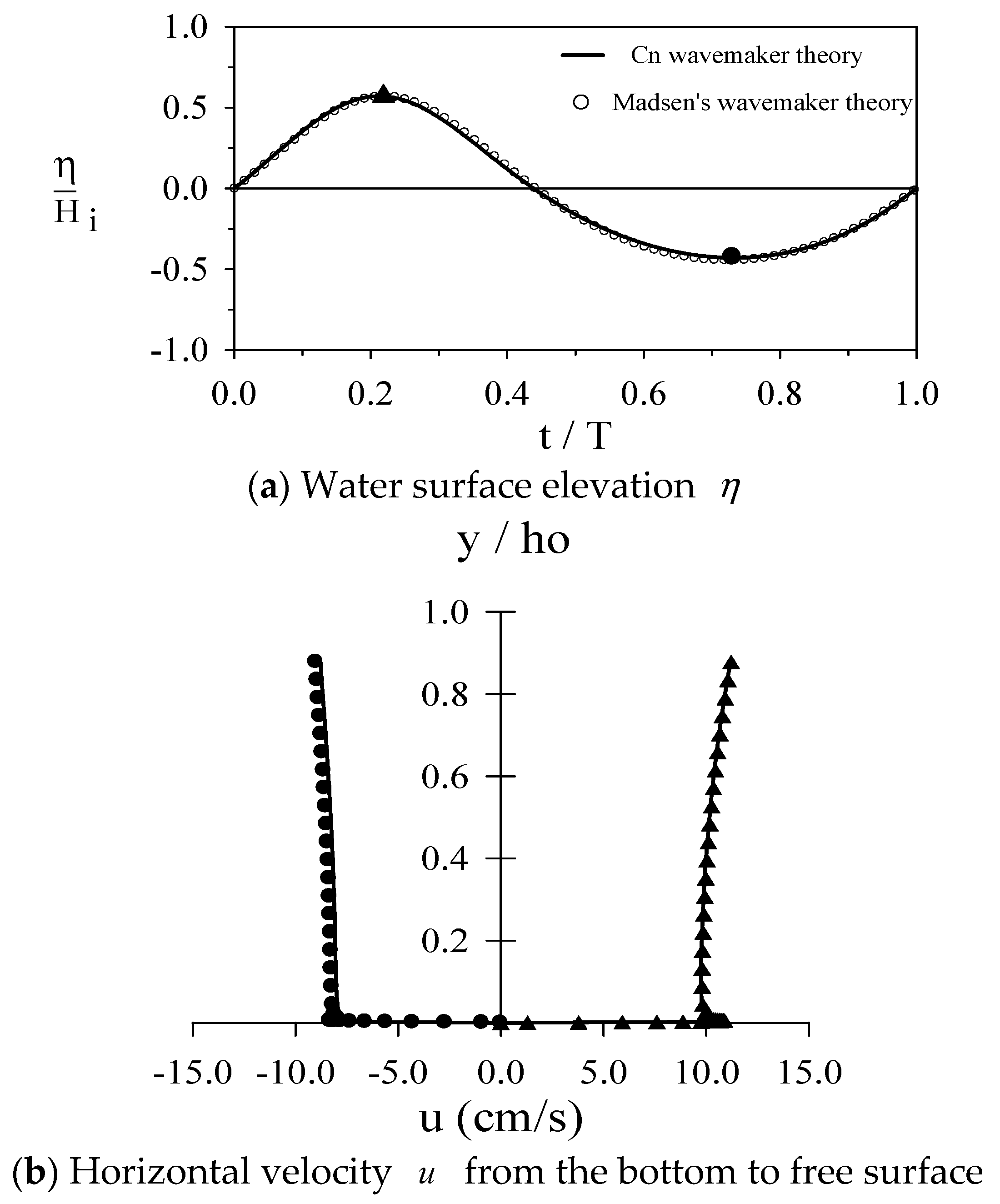
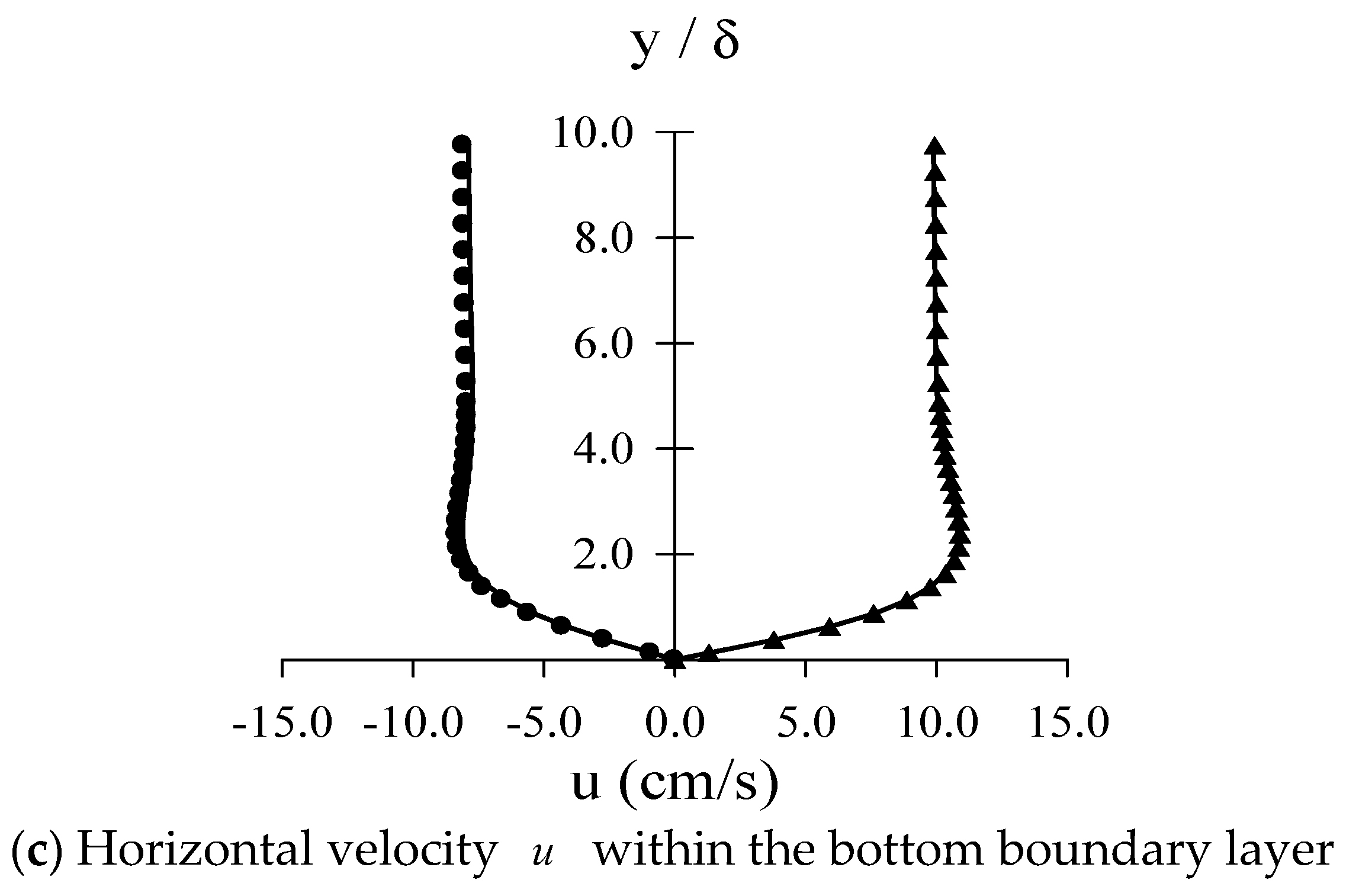
4.2. Verification of the Generated Cnoidal Waveforms and Flow Fields

This study focused on simulating the generation and long-distance propagation of cnoidal waves using a 2D viscous wave flume model. Six wave conditions were employed for the numerical experiments, as detailed in Table 1. Notably, the values of h o / L for waves in Cases 1 to 5 range from 0.068 to 0.195, indicating that these are intermediate-deep-water waves. Water waves are classified as intermediate-deep-water waves when h o / L values range from 0.05 to 0.5, or when k h o values are between π / 10 and π .
The Ursell number is a widely accepted parameter for quantifying the nonlinearity of waves propagating through water of finite depth. Accordingly, the waves in Case 1, with an Ursell number less than 1, are linear waves or small-amplitude waves, whereas those in Cases 2–5 are nonlinear or finite-amplitude waves. Case 6 represents a solitary wave; therefore, only the wave height and still water depth are provided. This study used the wave generation theory of Goring and Raichlen [8] to generate all types of waves (Cases 1–6). The waves in Case 5 have an Ursell number exceeding 26.32 and are referred to as cnoidal waves.
To ascertain the precision of the numerical model, the numerical results of the waveform and flow velocity of the cnoidal wave were compared with analytical solutions. This section specifically concentrates on the generation of cnoidal waves with ho = 0.4 m, T = 3.0 s, Hi = 8.0 cm, and U r = 43.81 (Case 5 in Table 1) in the numerical wave flume.
Figure 3a displays the surface elevation of the cnoidal wave with U r = 43.81 generated in the numerical wave flume, and Figure 3b depicts the associated horizontal velocity within the boundary layer induced by the cnoidal wave at the phases of the wave crest and trough. To facilitate a comparison, both the numerical and theoretical solutions are provided. Based on the formulation by Tanaka et al. [45], the horizontal velocity distribution within the boundary layer under a cnoidal wave can be expressed as follows:
u ( y ) = U c / B N n = 1 N a n [ cos ( n ω t ) exp ( β n y ) cos ( n ω t β n y ) ]
where Uc is the free-stream velocity far from the boundary layer at the wave crest, β n = n ω / ( 2 υ ) , and the coefficients BN and an can be expressed as follows:
B N = n = 1 N a n
a n = 1 2 k = 0 n 1 A k A n k 1 + k = 0 N n 1 A k A k + n
where
A k = α [ q k + 0.5 / ( 1 + q 2 k + 1 ) ]
The variable q in Equation (21) is the same as that in Equation (16). When U r 26.32 ,
α = 1 / q
and when U r > 26.32 ,
α = 4 / π ln   ( 1 / q )
The results presented in Figure 3a,b demonstrate good agreement between the numerical simulations and theoretical solutions for both the water surface profile of the cnoidal wave and the corresponding horizontal velocity within the boundary layer. Minor discrepancies observed in the surface elevation (Figure 3a) and horizontal velocity (Figure 3b) can be attributed to the following factors. In this study, for computational convenience, the square of the Jacobi elliptic cosine function, c n 2 , was approximated using a fifth-order Fourier series expansion (Equation (17), N = 5 ). Similarly, the horizontal velocity within the boundary layer for the cnoidal wave was calculated using Equation (18) with N = 5 . These discrepancies could be minimized by including additional terms (e.g., N = 10 ) in the Fourier series in Equation (17) to provide a more accurate input waveform and in Equation (18) to obtain a more precise velocity profile.

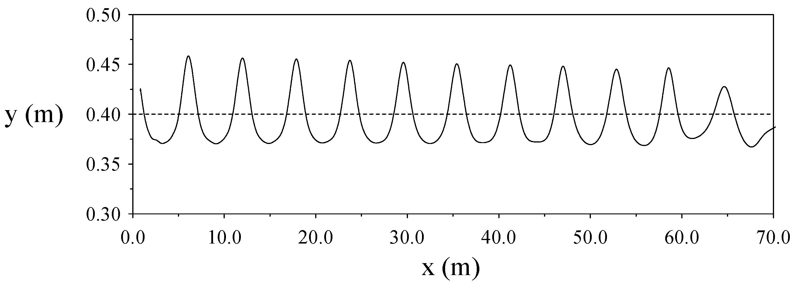
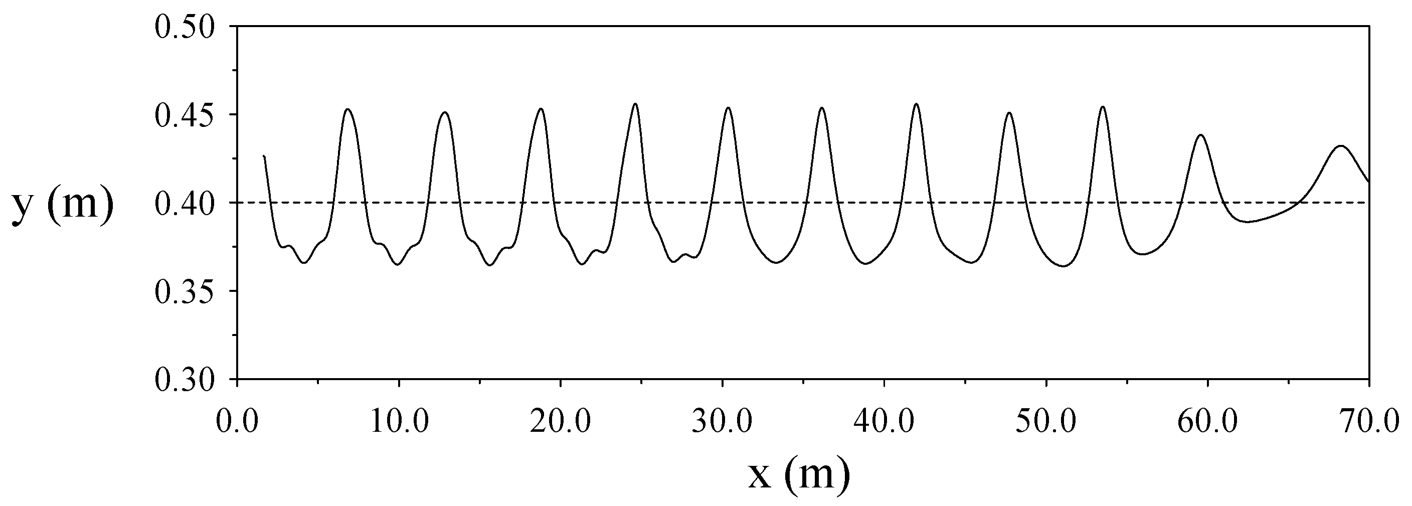
4.3. Examination of Permanent Waveform

To examine whether the cnoidal waves generated in the proposed numerical wave flume are permanent (that is, waveforms that do not change during wave propagation), the time series data of the water level at a distance of 10 m from the wavemaker for Case 5 was calculated (Figure 4). The cnoidal waves in the entire flume from x = 0 m to x = 70 m at time t = 33.3 s are shown in Figure 5. Figure 4 and Figure 5 collectively indicate that the cnoidal waves generated by the proposed numerical model exhibit regularity in both time and space without waveform variation during propagation.
The wave generation theory of Madsen [6] was also employed to generate waves for Case 5, and the results corresponding to those in Figure 4 and Figure 5 are presented in Figure 6 and Figure 7. These waves exhibit additional temporal and spatial components beyond the main frequencies of the waves. These additional components can be observed as secondary peaks in wave troughs and represent higher-order free waves. According to the dispersion relation, these waves, characterized by shorter periods, have smaller wave celerities than the main-frequency waves. Consequently, as the waves propagate, these components gradually separate from the main-frequency waves, resulting in supplementary peaks in the wave troughs, which can be seen in Figure 6 and Figure 7. This observation aligns with the findings of Buhr Hansen and Svendsen [7]. It has also been indicated in Section 3.1, for Stokes second-order waves when U r > 26.32 , bumps will appear in the wave troughs.

4.4. Comparison of Waves with U r < 26.32 Generated Using Various Methods

To gain further insights into potential distinctions in waves with U r < 26.32 generated using various wave generation theories, a comparative analysis was conducted for the waves in Case 1 ( U r = 0.67 ) and Case 3 ( U r = 13.98 ). In addition to cnoidal wavemaking theory, linear wave generation theory was employed to generate waves for Case 1, whereas Madsen’s theory was used to generate waves for Case 3.
Figure 8 compares the wave profiles and flow fields for waves in Case 1 generated using linear wavemaking theory against those obtained through cnoidal wave generation theory. The velocity field is depicted through horizontal velocity profiles extending from the bed to the free surface [Figure 8b], as well as within the near-bed boundary layer induced by wave motion [Figure 8c]. Some outliers observed in the bottom right corner of Figure 8b are attributed to the overshooting of velocity within the boundary layer (approximately from y / δ = 2 to 4), as highlighted in Figure 8c. Dong and Huang [16] validated that their simulated horizontal and vertical velocity fields near the bottom boundary closely aligned with theoretical predictions. In the figure, the triangle signifies the crest phase, and the circle represents the trough phase. The results depicted in Figure 8 reveal remarkable agreement in both the waveforms and flow velocities obtained using the two theories.
When the Ursell number is higher, linear wave generation theory tends to introduce higher-order free waves when generating finite-amplitude waves. To mitigate this effect, the wave generation theory of Madsen [6] was instead employed to generate the required wave series for Case 3 ( U r = 13.98 ).
Figure 9 showcases the outcomes for Case 3 waves generated using Madsen’s theory in comparison to cnoidal wave generation theory. The triangle and circle again represent the crest and trough phases, respectively. The results in Figure 9 reveal a close match between the two theories for both the waveform and flow field. Dong and Huang [14] showed that the numerical results for the horizontal velocity within the bottom boundary layer, induced by finite-amplitude waves as depicted in Figure 9c, were identical to the theoretical results obtained using the formula derived by Mizuguchi [40]. The results presented in Figure 8 and Figure 9, along with those in Figure 3, Figure 4 and Figure 5, suggest that when U r < 26.32 , cnoidal wave generation theory can effectively replace traditional linear or Madsen’s wave generation theories for producing regular waves using a piston-type wavemaker. Furthermore, when U r > 26.32 , cnoidal wave generation theory is the only one among the available theories capable of producing the required waves with a permanent waveform.

4.5. Generation of Solitary Wave

As mentioned above, when the modulus m of the Jacobi elliptic function equals 1, the cnoidal waveform transforms into a solitary waveform. Accordingly, the wavemaker motion described in Equation (7) can be applied to generate a solitary wave. In this study, as in Dong and Huang [16], Equation (7) was also applied to generate the solitary wave in Case 6 (Table 1). The resulting waveform and flow velocity are consistent with those reported by Dong and Huang [16]; for conciseness, these results are not presented here. Dong and Huang [16] also revealed that a solitary wave propagates stably in the channel. The attenuation of solitary wave amplitude due to fluid viscosity in a flat-bottomed channel was assessed and compared with analytical models developed by Keulegan [46] and Mei [47], as well as with experimental results reported by Russel [48].

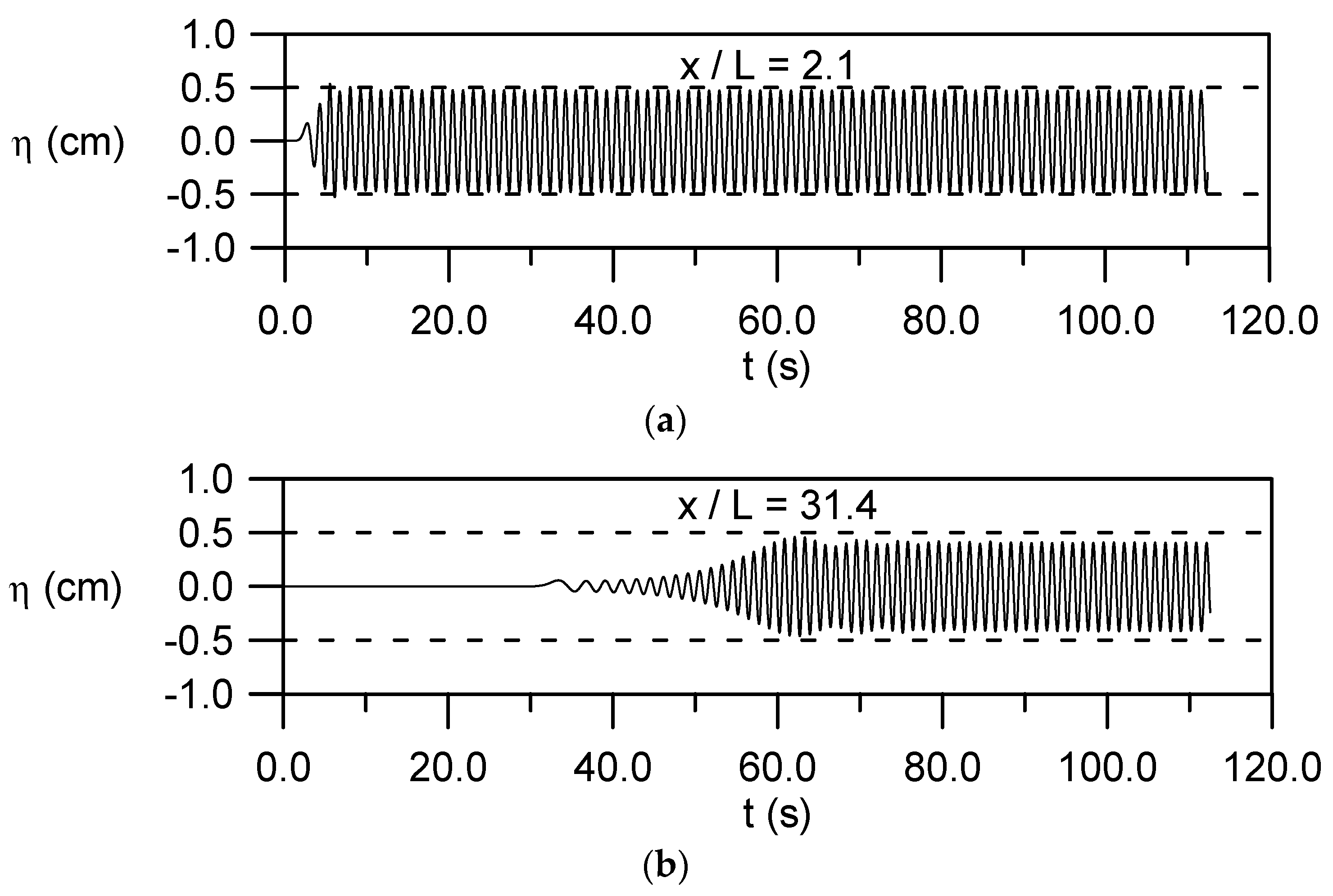
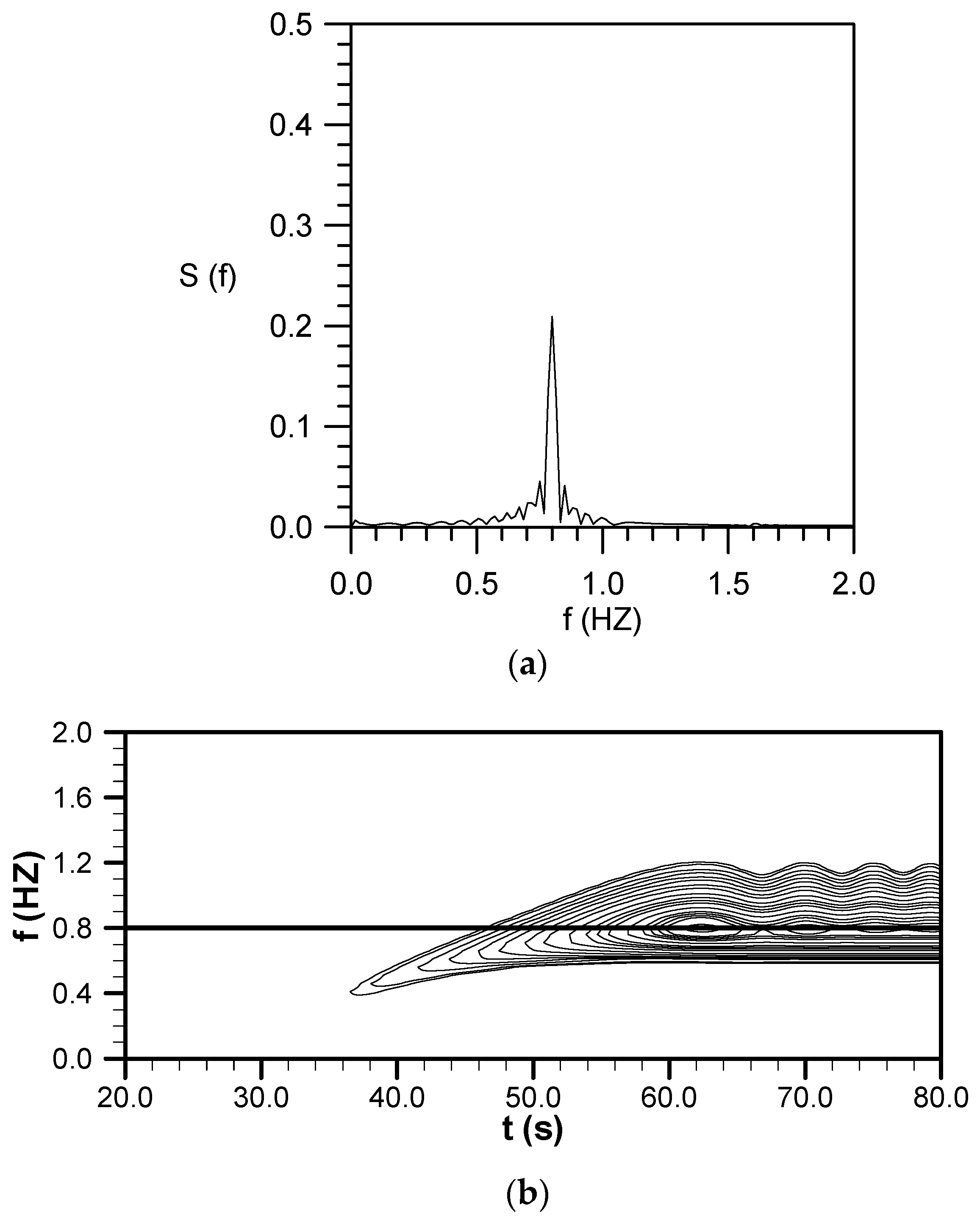
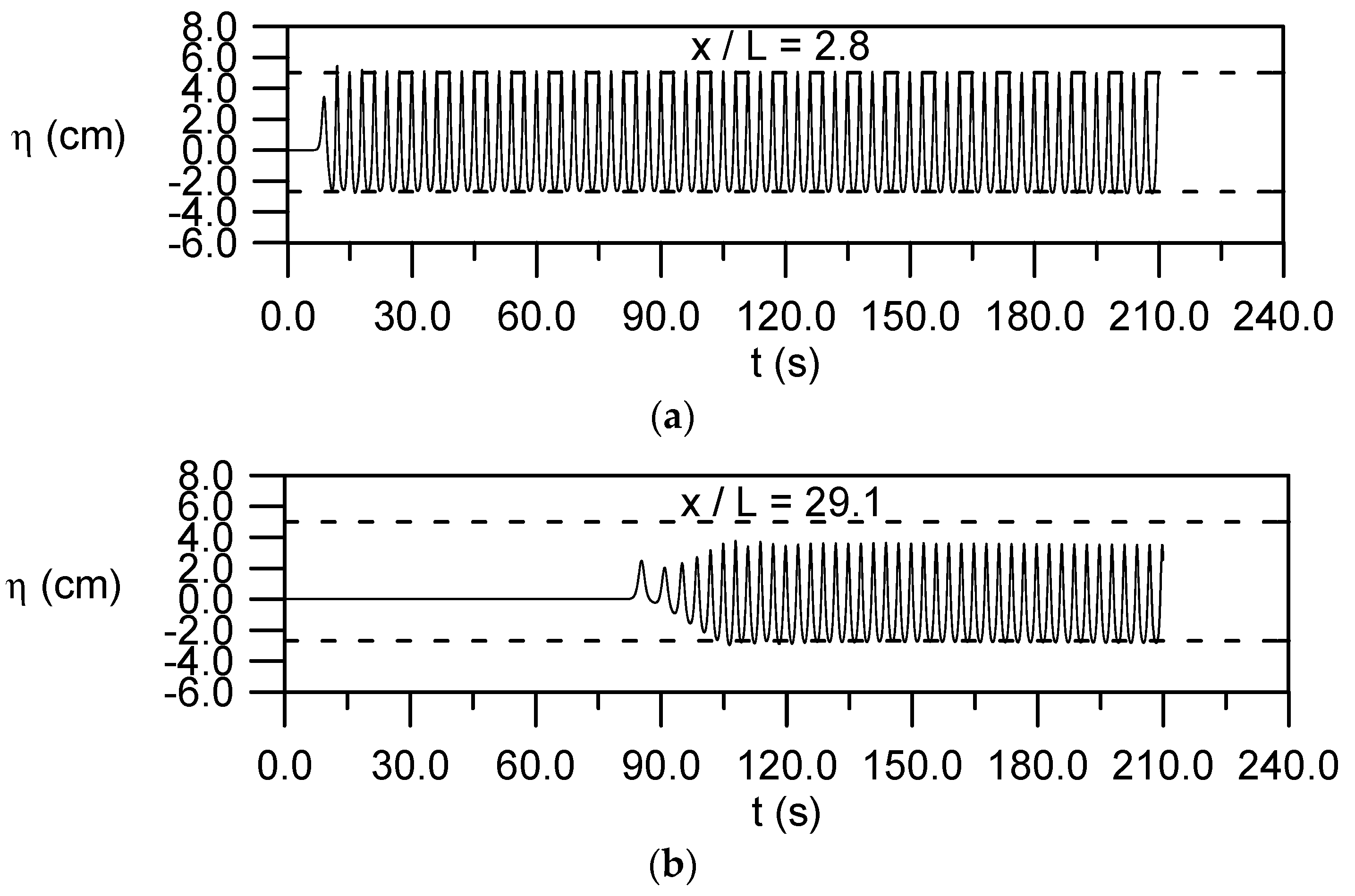
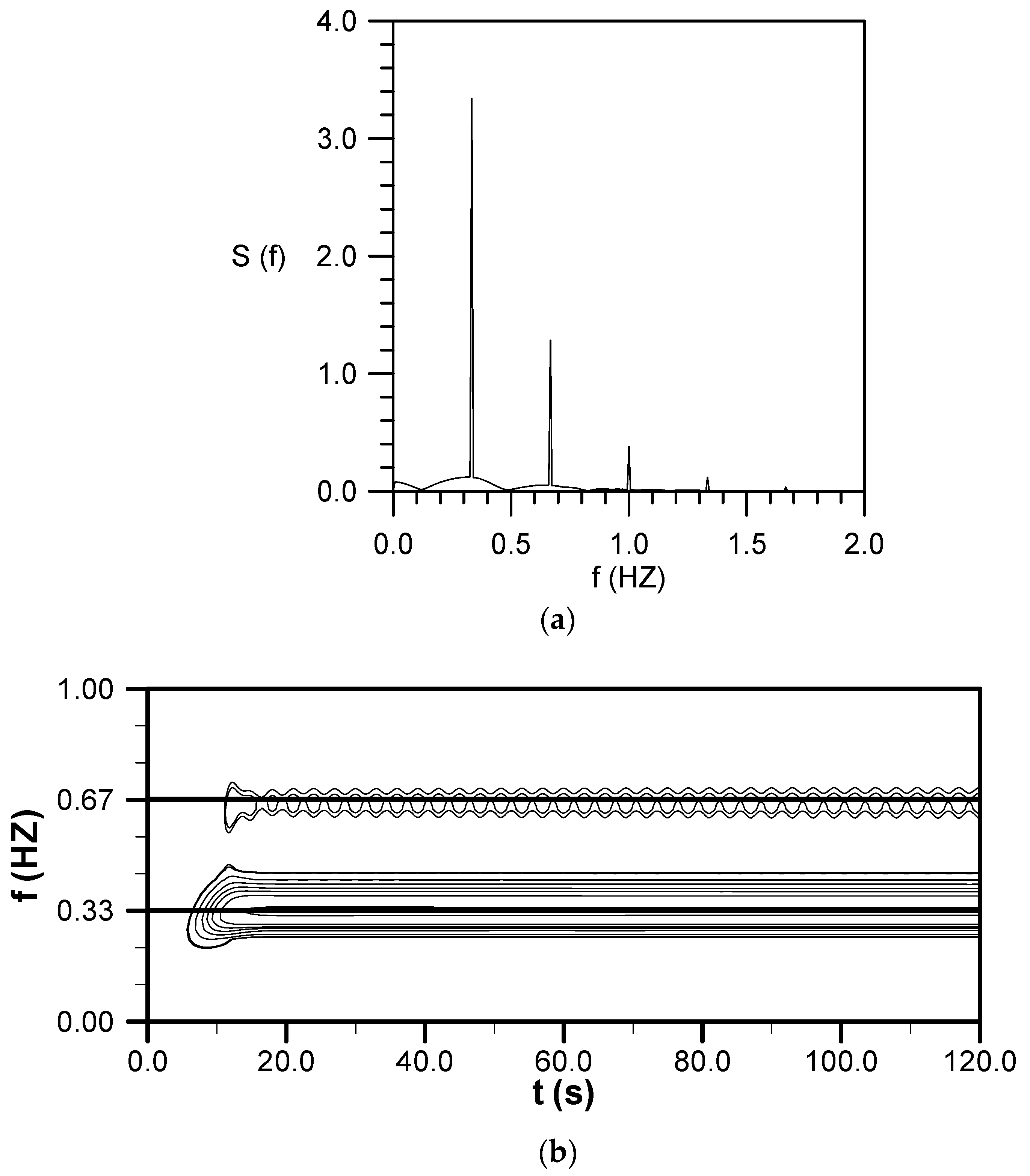
4.6. Evolution of a Small-Amplitude Wave Train with U r = 0.67

Dong and Huang [16] examined the evolution of wave trains generated in a 2D numerical viscous wave flume after prolonged propagation for small-amplitude waves (Case 1 in Table 1) and finite-amplitude waves with U r = 19.3 . The results in Figure 8 and Figure 9 demonstrate that when the wave generation theory of Goring and Raichlen [8] was applied, the small-amplitude waves produced matched those generated using linear wave-making theory. Similarly, the second-order Stokes waves were consistent with those generated using Madsen’s [6] wavemaking theory. This section investigates whether the evolution of a small-amplitude wave train with U r = 0.67 generated using Goring and Raichlen’s [8] theory is consistent with the findings of Dong and Huang [16].
Figure 10a,b show the time series of water levels at distances of 2.1 and 31.4 times the wavelength (L = 2.05 m), respectively, for Case 1. The figures clearly indicate that, as the wave train propagates, the wave height slightly decreases due to energy dissipation caused by viscosity. Additionally, wave trains gradually evolve to exhibit envelope-like waves at their front edges.
To delve deeper into the underlying mechanism, the time-series data of water level in Figure 10a,b were analyzed using both the Fourier transform and the Morlet wavelet transform [49,50]. The corresponding results are presented in Figure 11 and Figure 12. Figure 11a shows the wave spectral density, S ( f i ) , which is related to the amplitude at each frequency, a i . This relationship can be expressed as:
a i = 2 S ( f i ) Δ f
where Δ f represents the frequency resolution. The total wave energy can be calculated by summing the squared magnitudes of the amplitudes at each frequency, a i . The sideband frequencies observed near the primary 0.8 Hz peak in Figure 11a result from aliasing effects in the Fourier transform, caused by the non-periodic nature of the wave data at the front of the wave train. This aliasing can be minimized or eliminated by applying a window function, like the Hanning function. Figure 11b demonstrates that the dominant wave frequency remains stable during propagation, with the fundamental frequency being 0.8 Hz.
The spectrum chart in Figure 12a shows that during the transmission of the wave train, in addition to the main frequency wave, sideband components gradually emerge on either side of the main frequency. The wavelet analysis in Figure 12b reveals low-frequency sidebands—characterized by longer wavelengths and higher phase speeds—preceding the main wave group and interacting with it to form envelope-like waves at the front edge, as shown in Figure 10b. In contrast, the high-frequency sideband components, with shorter periods and slower speeds, trail behind the original wave train, as evidenced by their later appearance in the wavelet spectrum chart. These wave propagation characteristics are the same as those reported by Dong and Huang [16], who generated waves using linear wave generation theory.
In addition to the sideband frequencies, the spectral density of the fundamental frequency in Figure 12a is noticeably lower than that in Figure 11a. This difference can be attributed to two factors. First, part of the wave energy is dissipated due to viscous friction, as indicated by the reduced wave height in Figure 10b compared to Figure 10a. Second, some of the wave energy is transferred from the fundamental frequency to the sideband components.
The sideband components that emerge at the front of the wave train after a long period of propagation should be irrelevant to the evanescent-mode waves generated by the wavemaker. Because this evanescent mode decays exponentially and becomes negligible after a distance of three water depths from the wavemaker [1]. Furthermore, the sideband components appear only after the wave train has propagated for a long distance. The mechanism underlying the wave transformation depicted in Figure 10b can be described as follows: The nonhomogeneous leading waves in Figure 10a, which have frequencies slightly different from the main wave train, act as disturbances. Over prolonged propagation, interactions between the main waves and these disturbances give rise to sideband wave components. These components ultimately contribute to the emergence of envelope-like waves at the leading edge of the wave train.

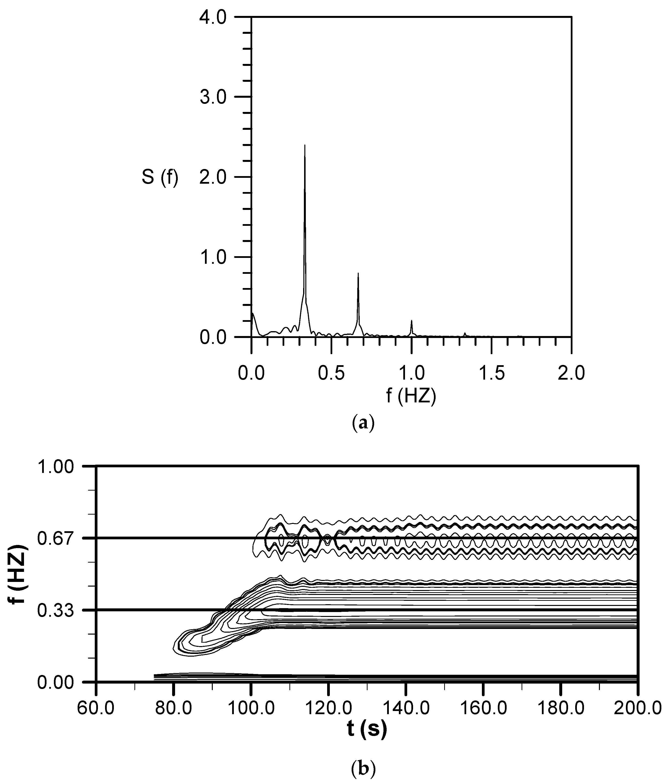
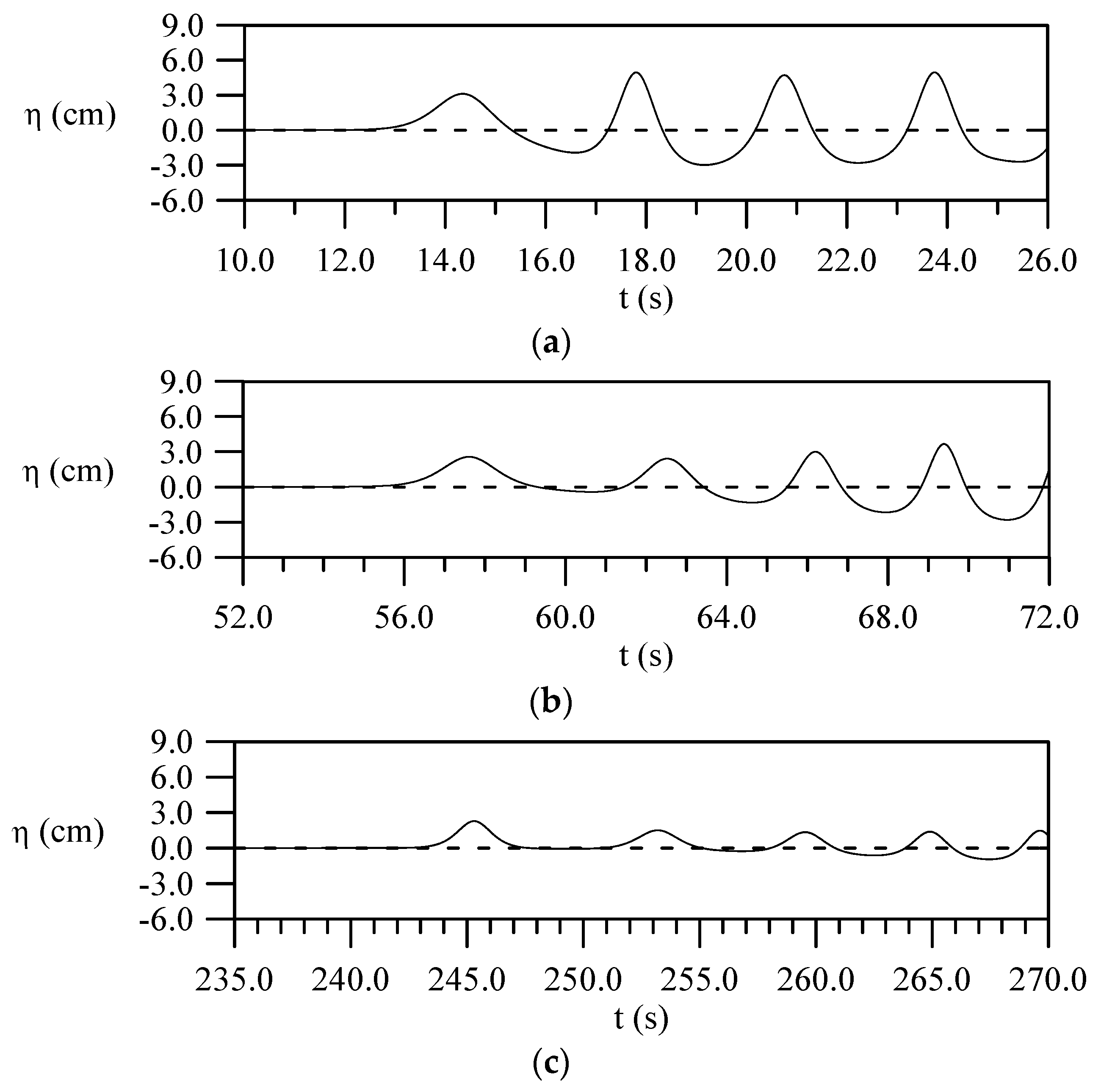
4.7. Evolution of a Cnoidal Wave Train with U r = 43.81

After verifying the accuracy of the numerical results for the generated cnoidal waves and the corresponding flow fields (Figure 3), and confirming that these waves propagate in a permanent form (Figure 4 and Figure 5), this section explores the long-term evolution of the cnoidal wave train during extended propagation in a 2D numerical viscous wave flume. Figure 13a,b illustrate the time series of water levels for Case 5 at distances of 2.8 and 29.1 times the wavelength ( L = 5.92 m ). It is noteworthy that the cnoidal waves remain stable during propagation, except at the leading edge of the wave train. While previous studies [34,35,36] have confirmed the stability of cnoidal waves during propagation, the behavior of the leading waves in a cnoidal wave train remains unexamined. In contrast to the case presented in Figure 10b, no front-edge envelope waves are observed in this case.
Figure 14 and Figure 15 illustrate the Fourier transform and wavelet transform charts for the water level time series at the two specified locations. Figure 14a indicates that at x / L = 2.8 , the cnoidal waves comprise five harmonics with frequencies of 0.33, 0.67, 1.00, 1.33, and 1.67 Hz. This observation suggests that second-order Stokes wave generation theory is inadequate for generating this wave, necessitating the application of cnoidal wave generation theory instead.
At x / L = 29.1 , the wave amplitude decreases due to energy dissipation caused by viscosity, resulting in a reduction in the spectral density of each harmonic and rendering the fifth harmonic indistinguishable, as shown in Figure 15a. Furthermore, the spectral and wavelet spectrum charts for this location reveal the emergence of a very low-frequency component, approximately at 75 s [see Figure 15b]. This timing aligns closely with the arrival of the leading edge of the wave train at the location x / L = 29.1 [refer to Figure 13b and Figure 15b]. This phenomenon indicates that, during transmission, the wave train generates a long wave with a significantly extended period at its leading edge, which is also evident in Figure 13b.
To investigate the formation and behavior of long waves at the leading edge of a cnoidal wave train, Figure 16a–c display the time series of the surface elevation at the front of the waves in Case 5 at three locations: (a) x = 4.7 L , (b) x = 19.6 L , and (c) x = 84.1 L , respectively. The results shown in Figure 16 reveal that, as the wave train travels, the leading waves develop into a series of solitary waves with a frequency approaching zero or a very long period, as indicated in Figure 15a,b. This characteristic becomes more apparent as the wave train moves further from the wavemaker. Furthermore, the leading solitary wave in Figure 16c has a greater height than the succeeding ones.
Notably, the leading wave of the wave train in Figure 16b resembles a solitary wave. If it travels as a solitary wave, its speed is 2.037 m/s [ c = g ( h o + H ) , where g is the gravitational acceleration of 9.81 m/s2, h o is the still water depth of 0.4 m, and H is the local solitary wave height of 2.31 cm]. At this speed, the leading wave would take 187.5 s to move from x = 19.6 L to x = 84.1 L ( L = 5.92 m ). Figure 16b,c shows that the actual difference in the time it takes the leading wave crest to travel between these two locations is 187.7 s, which is slightly longer than the estimated time of 187.5 s. The discrepancy arises because the wave height decreases during propagation, resulting in slightly lower wave speed and a slightly longer travel time than estimated. This observation demonstrates that the leading wave of the wave train behaves like a solitary wave.
Validating the evolution of the leading waves at the front of a cnoidal wave train into solitary waves in a physical wave flume is difficult because an extremely long flume is required. The phenomenon of the waves in a train disintegrating into a series of leading solitary waves has been reported. Several researchers [51,52] found that if the initial surface displacement integrates to have a positive volume, the wave train eventually disintegrates into a series of solitary waves with the tallest wave in front. The behaviors of the leading solitary waves observed in Figure 16c are consistent with these observations. To date, no theoretical or experimental investigations have been conducted on the evolution of the leading waves in a cnoidal wave train after a long period of propagation. A possible mechanism for the wave evolution observed in Figure 16 is suggested herein. Both solitary waves and cnoidal waves are solutions to the KdV equation. Boyd [53] showed that an infinite series of spatially repeated solitary waves is a first-order approximation to cnoidal waves. Consequently, the sideband component in a cnoidal wave train with a longer period and higher speed separates from the wave train and gradually becomes a sequence of solitary waves ordered by amplitude, as illustrated in Figure 16. As aforementioned, Benjamin [32], Pego and Weinstein [33], and Dong and Huang [16] showed that solitary waves can propagate stably within a channel. Consequently, once the front segment of a cnoidal wave train evolves into solitary waves, they continue traveling without changing shape.

4.8. Effect of Viscosity on Water Wave Motion and Advantage of a Viscous Wave Flume

As noted in the Introduction, Lamb [12] stated that viscosity has only a relatively minor effect on free oscillatory waves in deep water. However, he also pointed out that this estimation becomes invalid when the water depth is less than approximately half the wavelength. In this study, the waves fall into the intermediate-deep water category, with h o / L values ranging from 0.068 to 0.195—well below the 0.5 threshold. Therefore, although viscosity may not be the dominant factor, it cannot be entirely neglected.
This study accounts for fluid viscosity in wave generation and propagation by solving the Navier–Stokes equations. The results presented in Section 4.5, Section 4.6 and Section 4.7 show that the primary effect of viscosity is energy dissipation, which leads to a gradual reduction in wave height during propagation. The model’s accuracy in simulating wave height attenuation has been validated by Dong and Huang [16] for the case of a solitary wave.
Beyond wave height attenuation, the 2D numerical viscous wave flume developed in this study can simulate a wide range of incident wave conditions, including small- and large-amplitude waves, solitary waves, and cnoidal waves. This capability allows for the investigation of realistic viscous flow fields generated by waves and their interactions with structures. As a result, key physical phenomena—such as bottom shear stresses, vortex shedding, and frictional drag—can be accurately captured. These factors are essential for understanding sediment transport and wave–structure interactions.

5. Conclusions

This study combined the wave generation framework proposed by Goring and Raichlen [8] with the 2D viscous wave flume model developed by Dong and Huang [16] to simulate cnoidal waves. The characteristics of wave transformation after long propagation of the wave train were also investigated. The research findings are as follows:
For all studied waves within the Ursell number range 0.67 < U r < 43.81 , the waveforms and associated horizontal velocities from the bottom to the free surface, as well as within the bottom boundary layer, were consistent with the theoretical solutions.
At U r < 26.32 , cnoidal wave generation theory is a suitable replacement for traditional linear wave generation theory and the wave generation theory of Madsen [6] for generating small- and finite-amplitude waves, respectively.
At U r > 26.32 ( U r = 43.81 ), the waves generated throughout an entire flume by using cnoidal wave generation theory were regular in both time and space, whereas those produced using Madsen’s wave generation theory did not have permanent waveforms. This observation is consistent with the findings of Buhr Hansen and Svendsen [7].
Under small-amplitude wave conditions ( U r = 0.67 ), the wave train preserves its form during propagation; however, envelope-like waves gradually emerge at the leading edge after extended travel. Fourier transform and wavelet transform analyses revealed the presence of sideband components near the fundamental frequency. The interaction between these sideband components and the fundamental frequency wave is responsible for the formation of fenvelope-like waves. These propagation characteristics align with findings previously reported by Dong and Huang [16], who studied waves generated using linear wave generation theory.
For cnoidal waves with U r = 43.81 , the waves maintain stability over an extended period of propagation. However, the leading waves in the wave train gradually evolve into a series of solitary waves with near-zero frequency, with the tallest wave appearing at the front. Validating this phenomenon would require an exceptionally long physical wave flume. While this study explored potential reasons for this wave transformation, further investigation is needed to fully understand the underlying mechanisms.
In this study, only one case of cnoidal waves with U r = 43.81 was investigated. To draw comprehensive conclusions about the evolution of cnoidal waves across the full range of U r > 26.32 , further investigations with significantly higher Ursell numbers (e.g., U r = 300 and beyond) are required.

Author Contributions

Conceptualization, C.-J.H.; Methodology, C.-M.D. and C.-J.H.; Software, H.-C.H.; Validation, C.-M.D. and H.-C.H.; Investigation, C.-M.D., C.-J.H. and H.-C.H.; Writing—original draft, C.-M.D. and H.-C.H.; Writing—review & editing, C.-J.H. All authors have read and agreed to the published version of the manuscript.

Funding

This research received no external funding.

Data Availability Statement

The original contributions presented in this study are included in the article. Further inquiries can be directed to the corresponding author.

Conflicts of Interest

The authors declare no conflict of interest.

References

  1. Dean, R.G.; Dalrymple, R.A. Water Wave Mechanics for Engineers and Scientist; Prentice-Hall: Englewood Cliffs, NJ, USA, 1984. [Google Scholar]
  2. Havelock, T.H. Forced surface wave on water. Lond. Edinb. Dublin Philos. Mag. J. Sci. 1929, 7, 569–576. [Google Scholar] [CrossRef]
  3. Ursell, F.; Dean, R.G.; Yu, Y.S. Forced small-amplitude water waves: A comparison of theory and experiment. J. Fluid Mech. 1960, 7, 32–53. [Google Scholar] [CrossRef]
  4. Hudspeth, R.T.; Leonard, J.W.; Chen, M.C. Design curves for hinged wave makers: Experiments. J. Hydraul. Div. Am. Soc. Civ. Eng. 1981, 107, 533–574. [Google Scholar]
  5. Goda, Y. Traveling Secondary Wave Crests in Wave Channels; Rep. No. 13; Port & Harbor Research Institute: Yokosuka, Japan, 1967; pp. 32–38. [Google Scholar]
  6. Madsen, O.S. On the generation of long waves. J. Geophys. Res. 1971, 76, 8672–8683. [Google Scholar] [CrossRef]
  7. Buhr Hansen, J.; Svendsen, I.A. Regular Waves in Shoaling Water—Experimental Data; Series Paper 21; ISVA, Technical University of Denmark: Kongens Lyngby, Denmark, 1974. [Google Scholar]
  8. Goring, D.; Raichlen, F. The generation of long waves in the laboratory. In Proceedings of the 17th Coastal Engineering Conference, Sydney, Australia, 23–28 March 1980; pp. 763–783. [Google Scholar]
  9. Ohyama, T.; Nadaoka, K. Development of a numerical wave tank for analysis of nonlinear and irregular wave field. Fluid Dyn. Res. 1991, 8, 231–251. [Google Scholar] [CrossRef]
  10. Grilli, S.T.; Horillo, J. Numerical generation and absorption of fully nonlinear periodic waves. J. Eng. Mech. 1997, 123, 1060–1069. [Google Scholar] [CrossRef]
  11. Guyenne, P.; Nicholls, D.P. A high-order spectral method for nonlinear water waves over moving bottom topography. SIAM J. Sci. Comput. 2007, 30, 81–101. [Google Scholar] [CrossRef]
  12. Lamb, H. Hydrodynamics, 6th ed.; Dover Publications: New York, NY, USA, 1945; pp. 623–625. [Google Scholar]
  13. Huang, C.J.; Dong, C.M. Wave deformation and vortex generation in water waves propagating over a submerged dike. Coast. Eng. 1999, 37, 123–148. [Google Scholar] [CrossRef]
  14. Huang, C.J.; Dong, C.M. On the interaction of a solitary wave and a submerged dike. Coast. Eng. 2001, 43, 265–286. [Google Scholar] [CrossRef]
  15. Huang, C.J.; Zhang, E.C.; Lee, J.F. Numerical simulation of nonlinear viscous wavefields generated by a piston-type wavemaker. J. Eng. Mech. 1998, 124, 1110–1120. [Google Scholar] [CrossRef]
  16. Dong, C.M.; Huang, C.J. Generation and propagation of water waves in a two-dimensional numerical viscous wave flume. J. Waterw. Port Coast. Ocean Eng. 2004, 130, 143–153. [Google Scholar] [CrossRef]
  17. Madsen, P.A.; Fuhrman, D.R.; Schäffer, H.A. On the solitary wave paradigm for tsunamis. J. Geophys. Res. 2008, 113, C12012. [Google Scholar] [CrossRef]
  18. Lin, P.; Liu, P.L.-F. Internal wave-maker for Navier-Stokes equations models. J. Waterw. Port Coast. Ocean Eng. 1999, 125, 207–215. [Google Scholar] [CrossRef]
  19. Liu, J.; Hayatdavoodi, M.; Ertekin, R.C. A comparative study on generation and propagation of nonlinear waves in shallow waters. J. Mar. Sci. Eng. 2023, 11, 917. [Google Scholar] [CrossRef]
  20. Green, A.E.; Naghdi, P.M. A derivation of equations for wave propagation in water of variable depth. J. Fluid Mech. 1976, 78, 237–246. [Google Scholar] [CrossRef]
  21. Keulegan, G.H.; Patterson, J.A. Mathematical theory of irrotational translation waves. J. Res. Natl. Bur. Stand. 1940, 24, 47–101. [Google Scholar] [CrossRef]
  22. Korteweg, D.J.; de Vries, G. On the change of form of long waves advancing in a rectangular canal and on a new type of long stationary waves. Philos. Mag. 1895, 39, 422–443. [Google Scholar] [CrossRef]
  23. Dingemans, M.W. Water wave propagation over uneven bottoms: Linear wave propagation. Adv. Ser. Ocean. Eng. 1997, 13, 708–715. [Google Scholar]
  24. Greenshields, C.J. OpenFOAM User Guide, Version 6; OpenFOAM Found. Ltd.: London, UK, 2018.
  25. Svendsen, I.A.; Brink-Kjær, O. Shoaling of cnoidal waves. In Proceedings of the 13th Coastal Engineering Conference, Vancouver, BC, Canada, 10–14 July 1972; pp. 365–384. [Google Scholar]
  26. Synolakis, C.E.; Deb, M.K. On the maximum runup of cnoidal waves. In Proceedings of the 21th Coastal Engineering Conference, Malaga, Costa del Sol, Spain, 20–25 June 1988; pp. 553–565. [Google Scholar]
  27. Lee, T.C.; Tang, C.J. Numerical study on generation of cnoidal waves and induced viscous flow over a wavy bed. In Proceedings of the 19th International Offshore and Polar Engineering Conference, Osaka, Japan, 21–26 June 2009; pp. 846–853. [Google Scholar]
  28. Benjamin, T.B.; Feir, J.E. The disintegration of wave trains on deep water. Part 1. Theory. J. Fluid Mech. 1967, 27, 417–430. [Google Scholar] [CrossRef]
  29. Su, M.Y.; Bergin, M.; Marler, P.; Myrick, R. Experiments on nonlinear instabilities and evolution of steep gravity wave trains. J. Fluid Mech. 1982, 124, 45–72. [Google Scholar] [CrossRef]
  30. Benjamin, T.B. Instability of periodic wavetrains in nonlinear dispersive systems. Proc. R. Soc. Lond. A 1967, 299, 59–76. [Google Scholar]
  31. Whitham, G.B. Non-linear dispersion of water waves. J. Fluid Mech. 1967, 27, 399–412. [Google Scholar] [CrossRef]
  32. Benjamin, T.B. The stability of solitary waves. Proc. R. Soc. Lond. A 1972, 328, 153–183. [Google Scholar]
  33. Pego, R.L.; Weinstein, M.I. Asymptotic stability of solitary waves. Commun. Math. Phys. 1994, 164, 305–349. [Google Scholar] [CrossRef]
  34. Angulo Pava, J.; Bona, J.L.; Scialom, M. Stability of cnoidal waves. Adv. Differ. Eq. 2006, 11, 1321–1374. [Google Scholar] [CrossRef]
  35. Bottman, N.; Deconinck, B. KdV cnoidal waves are spectrally stable. Discret. Cont. Dyn. Syst. 2009, 25, 1163–1180. [Google Scholar] [CrossRef]
  36. Deconinck, B.; Kapitula, T. The orbital stability of the cnoidal waves of the Korteweg-de Vries equation. Phys. Lett. A 2010, 374, 4018–4022. [Google Scholar] [CrossRef]
  37. Chen, C.J.; Chen, H.C. The Finite-Analytic Method; IIHR Rep. No. 232-IV; IIHR—Hydroscience & Engineering, The University of Iowa: Iowa City, IA, USA, 1982. [Google Scholar]
  38. Patankar, S.V. Numerical Heat Transfer and Fluid Flow; McGraw-Hill Inc.: New York, NY, USA, 1980. [Google Scholar]
  39. Chan, R.K.; Street, R.L. A computer study of finite-amplitude water waves. J. Comput. Phys. 1970, 6, 95–104. [Google Scholar] [CrossRef]
  40. Mizuguchi, M. Second-order solution of laminar boundary layer flow under waves. Coast. Eng. Jpn. 1987, 30, 9–18. [Google Scholar] [CrossRef]
  41. Mei, C.C.; Stiassine, M.; Yue, D.K.-P. Theory and Applications of Ocean Surface Waves. Part 2: Nonlinear Aspects; World Scientific Publishing Co. Pte. Ltd.: Singapore, 2005; Chapter 12. [Google Scholar]
  42. Byrd, P.F.; Friedman, M.D. Handbook of Elliptic Integrals for Engineers and Scientists, 2nd ed.; Springer: New York, NY, USA, 1971. [Google Scholar]
  43. Isobe, M. Calculation and application of first-order cnoidal wave theory. Coast. Eng. 1985, 9, 309–325. [Google Scholar] [CrossRef]
  44. Kiper, A. Fourier series coefficients for powers of the Jacobian elliptic functions. Math. Comput. 1984, 43, 247–259. [Google Scholar] [CrossRef]
  45. Tanaka, H.; Sumer, B.M.; Lodahl, C. Theoretical and experimental investigation on laminar boundary layers under cnoidal wave motion. Coast. Eng. Jpn. 1998, 40, 81–98. [Google Scholar] [CrossRef]
  46. Keulegan, G.H. Gradual damping of solitary waves. J. Res. Natl. Bur. Stand. 1948, 40, 487–498. [Google Scholar] [CrossRef]
  47. Mei, C.C. The Applied Dynamics of Ocean Surface Waves; Wiley: New York, NY, USA, 1983. [Google Scholar]
  48. Russel, J.S. Report of the Committee on waves. In Report of the 7th Meeting of British Association for the Advancement of Science; John Murray: London, UK, 1838; pp. 417–496. [Google Scholar]
  49. Grossmann, A.; Morlet, J. Decomposition of Hardy functions into square integrable wavelets of constant shape. SIAM J. Math. Anal. 1984, 15, 723–736. [Google Scholar] [CrossRef]
  50. Young, R.K. Wavelet Theory and Its Applications; Kluwer Academic Publishers: Boston, MA, USA, 1993. [Google Scholar]
  51. Hammack, J.L.; Segur, H. The Korteweg–de Vries equation and water waves. Part 2: Comparison with experiments. J. Fluid Mech. 1974, 65, 289–314. [Google Scholar] [CrossRef]
  52. Goring, D.G. Tsunamis—The Propagation of Long Waves onto a Shelf; Rep. Kh-R-38; W. M. Keck Laboratory of Hydraulics and Water Resources, California Institute of Technology: Pasadena, CA, USA, 1978. [Google Scholar]
  53. Boyd, J.P. Cnoidal waves as exact sums of repeated solitary waves: New series for elliptic functions. SIAM Appl. Math. 1984, 44, 952–955. [Google Scholar] [CrossRef]
Figure 1. Schematic of a 2D numerical wave flume with a flat bottom and a piston-type wavemaker.
Jmse 13 01102 g001
Figure 2. Comparison of the square of the Jacobi elliptic cosine function c n 2 and the approximations synthesized using first-to fifth-order Fourier series; (a) first to third order, (b) fourth to fifth order.
Jmse 13 01102 g002
Figure 3. (a) Surface elevation of the cnoidal wave with U r = 43.81 (Case 5 in Table 1) generated in the numerical wave flume and (b) the associated horizontal velocity within the boundary layer at the phases of the wave crest and trough. The line represents the numerical solution, and the circle and triangle symbols represent the theoretical solutions at the wave crest and trough, respectively.
Jmse 13 01102 g003
Figure 4. Time-series data of the water surface elevation at x = 10 m, generated using cnoidal wavemaking theory for the waves in Case 5 with U r = 43.81 .
Jmse 13 01102 g004
Figure 5. Cnoidal waves with U r = 43.81 in the entire flume, generated using cnoidal wavemaking theory from x = 0 m to x = 70 m at time t = 33.3 s.
Jmse 13 01102 g005
Figure 6. Time-series data of water surface elevation at x = 10 m, generated using Madsen’s wavemaking theory for the waves in Case 5 with U r = 43.81 .
Jmse 13 01102 g006
Figure 7. Cnoidal waves with U r = 43.81 in the entire flume, generated using Madsen’s wavemaking theory from x = 0 m to x = 70 m at time t = 33.3 s.
Jmse 13 01102 g007
Figure 8. Comparison of wave profiles and flow fields for waves in Case 1 ( U r = 0.67 ) generated through linear wavemaking theory with those obtained through cnoidal wave generation theory: (a) wave profile, (b) horizontal velocity from the bottom to the free surface, and (c) horizontal velocity within the bottom boundary layer.
Jmse 13 01102 g008
Figure 9. Comparison of wave profiles and flow fields for waves in Case 3 ( U r = 13.98 ) generated using Madsen’s wavemaking theory with those obtained through cnoidal wave generation theory: (a) wave profile, (b) horizontal velocity from the bottom to the free surface, and (c) horizontal velocity within the bottom boundary layer.
Jmse 13 01102 g009aJmse 13 01102 g009b
Figure 10. Time-series data of the water surface elevation at (a) x/L = 2.1 and (b) x/L = 31.4, generated using cnoidal wavemaking theory for the wave in Case 1 with L = 2.05 m.
Jmse 13 01102 g010
Figure 11. (a) Fourier transform and (b) wavelet transform of the time-series data of the surface elevation presented in Figure 10a ( x / L = 2.1 ).
Jmse 13 01102 g011
Figure 12. (a) Fourier transform and (b) wavelet transform of the time-series data of the surface elevation presented in Figure 10b ( x / L = 31.4 ).
Jmse 13 01102 g012
Figure 13. Time-series data of the water surface elevation at (a) x / L = 2.8 and (b) x / L = 29.1 , generated using cnoidal wavemaking theory for the wave in Case 5 with L = 5.92 m .
Jmse 13 01102 g013
Figure 14. (a) Fourier transform and (b) wavelet transform of the time-series data of the surface elevation presented in Figure 13a ( x / L = 2.8 ).
Jmse 13 01102 g014
Figure 15. (a) Fourier transform and (b) wavelet transform of the time-series data of the surface elevation presented in Figure 13b ( x / L = 29.1 ).
Jmse 13 01102 g015
Figure 16. Time series of the surface elevation at the front of the wave train in Case 5 at three locations: (a) x = 4.7 L , (b) x = 19.6 L , and (c) x = 84.1 L ( L = 5.92   m ).
Jmse 13 01102 g016
Table 1. Wave conditions for numerical experiments.
Variable T ( s ) H i ( cm ) h o ( m ) L   ( m ) h o L k h o U r   =   H i L 2 h o 3
Case 11.251.00.42.050.1951.2250.67
Case 22.02.00.43.690.1080.6794.31
Case 32.54.00.44.720.0850.53413.98
Case 43.05.00.45.770.0690.43325.91
Case 53.08.00.45.920.0680.42743.81
Case 6-12.00.4----
Disclaimer/Publisher’s Note: The statements, opinions and data contained in all publications are solely those of the individual author(s) and contributor(s) and not of MDPI and/or the editor(s). MDPI and/or the editor(s) disclaim responsibility for any injury to people or property resulting from any ideas, methods, instructions or products referred to in the content.

