A Multi-Time-Frequency Feature Fusion Approach for Marine Mammal Sound Recognition

Abstract

Accurate acoustic identification of marine mammals is vital for monitoring ocean health and human impacts. Existing methods often struggle with limited single-feature representations or suboptimal fusion of multiple features. This paper proposes an Evaluation-Adaptive Weighted Multi-Head Fusion Network that integrates CQT and STFT features via a dual-branch ResNet architecture. The model enhances intra-branch features using channel attention and adaptive weighting of each branch based on its validation accuracy during training. Experiments on the Watkins Marine Mammal Sound Database show that the proposed method achieves superior performance, reaching 96.05% accuracy and outperforming baseline and attention-based fusion models. This approach offers an effective solution for multi-feature acoustic recognition in complex underwater environments.

1. Introduction

The marine environment is increasingly affected by anthropogenic activities, notably vessel traffic, underwater acoustic communication, and military operations, which significantly impact marine ecosystems and adversely affect the behavior and physiology of marine animals [1]. In pursuit of biodiversity preservation and ecological equilibrium, research efforts are focused on fostering sustainable interactions between human activities and marine life. Mitigation measures aimed at reducing adverse effects include optimizing cargo vessel speeds [2], improving fishing methodologies [3], managing acoustic output during offshore construction [4], and developing cognitive acoustic networks to prevent spectral conflicts [5,6]. Crucially, the assessment of these mitigation strategies’ effectiveness, alongside ongoing environmental monitoring, relies heavily on accurate and efficient species identification within targeted regions, particularly for marine mammals acting as key indicator species. Consequently, marine bioacoustic identification emerges as a cornerstone task for both marine engineering and ecological conservation initiatives.

Marine mammals are highly sensitive to environmental changes and are thus often considered ideal subjects for evaluating marine ecosystem health [7,8]. Like many other marine animals, they rely heavily on sound for communication, navigation, and foraging [9]. Acoustic signals are particularly effective for monitoring and identifying marine mammals because sound waves experience significantly less energy attenuation in seawater compared to light waves, allowing for propagation over much greater distances [10]. Current acoustic identification methodologies typically integrate acoustic feature extraction with machine learning classifiers [11,12,13]. This automation significantly enhances processing efficiency and diminishes the need for specialized human listeners. Commonly utilized acoustic features encompass relatively simple time-domain characteristics (e.g., zero-crossing rate [14]) as well as frequency-domain features like Mel-frequency cepstral coefficients (MFCC) [15], Gammatone frequency cepstral coefficients (GFCC) [16], and wavelet transform features [17,18]. Furthermore, propelled by advancements in deep learning for image recognition, spectrogram representations (e.g., Mel spectrograms [19], Short-Time Fourier Transform (STFT) spectrograms [20], Constant-Q Transform (CQT) spectrograms [21]) have become mainstream inputs. These representations effectively visualize the time-varying spectral energy distribution of signals, making them particularly suitable for analyzing non-stationary underwater acoustic signals. Both the judicious selection of features and the subsequent architecture of the classification model are critical determinants of identification performance [22].

With the rapid advancement of machine learning, research in marine mammal recognition has evolved beyond relying on a single feature type. Increasingly, multiple complementary features are being integrated for multi-feature recognition. Cai et al. employed four distinct features as inputs to a parallel neural network, achieving a whale species recognition accuracy of 95.21% [23]. Lü et al. introduced delay-Doppler domain features into the task, effectively addressing the impact of seasonal variations in the marine environment on acoustic signals. When combined with Mel-frequency cepstral coefficient (MFCC) features in a dual-input neural network, the model achieved outstanding recognition performance [24]. González-Hernández et al. used octave-band analysis to extract acoustic features, attaining a 90% recognition accuracy for various underwater sound signals while maintaining computational efficiency [25]. Nadir M et al. fused one-dimensional Local Binary Pattern (1D-LBP) features with MFCCs and used a support vector machine (SVM) for classification, reaching 89.6% accuracy across six marine mammal recognition tasks [26]. Kirsebom et al. achieved 90% accuracy in recognizing North Atlantic right whales under varying environmental conditions using a two-dimensional convolutional network, and further demonstrated that high-variance datasets are beneficial for model training [27]. Wu et al. input two cepstrum-based features—average cepstral and cepstral liftering—into a custom multilayer perceptron neural network (MLPNN), achieving a 95.45% recognition rate in dolphin whistle classification [28].

These studies collectively indicate that integrating multiple complementary features has become an effective strategy for enhancing the performance of marine mammal recognition systems. However, while existing research highlights the advantages of multi-feature approaches, it often focuses on which features to combine, with relatively limited attention paid to how to effectively fuse them. Many studies still rely on simple concatenation or averaging methods. Therefore, exploring more advanced and adaptive feature fusion mechanisms holds great promise for further leveraging the synergistic potential of multi-feature integration.

In selecting an appropriate fusion architecture, the rationale lies in the complementary nature of the chosen features and the specific demands of the task. Short-Time Fourier Transform (STFT) spectrograms offer excellent temporal resolution, making them effective for capturing transient acoustic events, while Constant-Q Transform (CQT) spectrograms provide superior frequency resolution, especially suitable for analyzing the harmonically rich vocalizations of marine mammals. A dual-branch residual network (ResNet) architecture is thus a compelling choice. This design enables each type of feature representation to be processed through a dedicated deep convolutional pathway, preserving its unique structural characteristics before fusion. The use of ResNet is motivated by its demonstrated ability to extract robust, hierarchical features from 2D image-like data and to mitigate the vanishing gradient problem commonly encountered in deep neural networks [29]. Although powerful alternatives such as Transformer and LSTM networks were considered, they are more commonly used for one-dimensional sequence prediction tasks [30] and have limitations in this context. LSTM networks, being inherently sequential and designed for 1D temporal data, are less suited for modeling the complex 2D time-frequency patterns present in spectrograms [31]. On the other hand, Transformers typically require large-scale datasets and substantial computational resources due to their extensive parameterization and reliance on self-attention mechanisms that scale quadratically with input size. This makes them less practical for tasks with limited labeled data or constrained computational environments, as often encountered in underwater acoustic analysis [32]. Therefore, the dual-branch ResNet architecture was benchmarked as a more pragmatic and task-specialized solution for effectively fusing STFT and CQT spectrogram features.

To address the aforementioned issues and fully exploit the advantages of multi-feature fusion, this paper proposes an Evaluation-Adaptive Weighted Multi-Head Fusion Network (EAW-MHFN). The main contributions and innovations of this work are as follows:

• A dual-branch residual network architecture is proposed, which effectively leverages the complementarity between Constant-Q Transform (CQT) and Short-Time Fourier Transform (STFT) features for marine mammal sound recognition.
• A systematic exploration and comparison of different feature fusion strategies is conducted, including a simple concatenation baseline, an attention-based adaptive weighted fusion approach (used as a comparative model), and the proposed advanced fusion network.
• The EAW-MHFN is meticulously designed and implemented. It innovatively integrates channel attention (CA) within each branch, adaptive inter-branch weighting based on dynamic performance evaluation on the validation set, and a multi-head supervised learning strategy to enable more intelligent feature integration and a more optimized training process.

To validate the effectiveness of the proposed model in marine mammal acoustic recognition, a dataset was constructed using vocalizations from 12 dolphin species in the Watkins Marine Mammal Sound Database (WMMD) [33]. We conduct comprehensive performance comparisons with single-branch baseline models, simple concatenation-based fusion models, and attention-based fusion models. Additionally, ablation studies are performed to further assess the individual contributions of the proposed components.

2. Theory

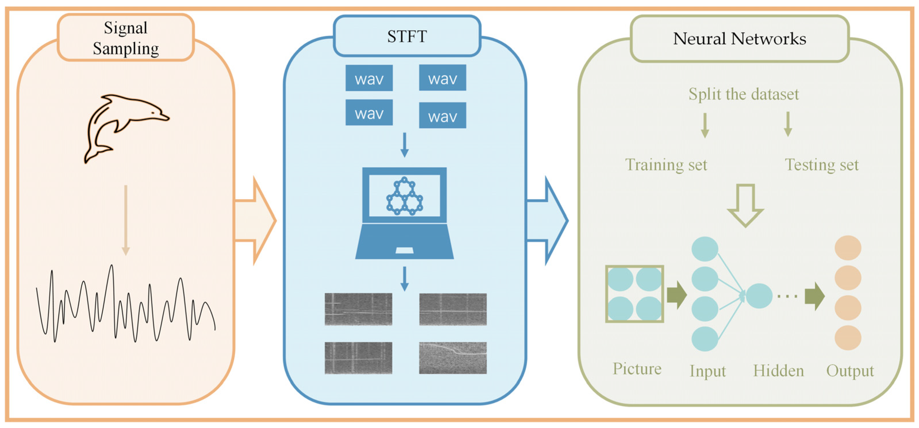
In this study, we adopt a mainstream acoustic feature recognition framework widely used in the field of acoustic signal processing [34] to perform marine mammal classification. By transforming raw audio signals into more informative time-frequency representations, these features are fed into a deep learning network, which automatically learns hierarchical feature representations through multiple layers of nonlinear transformations. Specifically, lower-level convolutional kernels capture local time-frequency patterns, while deeper network layers extract higher-level semantic features. Finally, a fully connected layer maps these features to class probabilities. The basic framework is illustrated in Figure 1.

The collected audio recordings are first resampled and then transformed into spectrogram features through signal processing. In this study, the Short-Time Fourier Transform (STFT) and Constant-Q Transform (CQT) spectrograms are computed using the torchaudio and nnAudio libraries, respectively. The resulting feature dataset is subsequently divided into training and testing sets according to a predefined ratio. The training set is used for learning feature representations, while the testing set is used to evaluate the model’s generalization performance. Training is conducted over multiple iterations, and the process is terminated once the experimental results converge and stabilize.

2.1. Time-Frequency Analysis of Marine Mammal Vocalizations

2.1.1. STFT Spectrogram

Spectrogram representation is one of the most commonly used techniques in one-dimensional signal analysis [35]. By applying the Short-Time Fourier Transform (STFT) to long-duration signals, a corresponding STFT spectrogram can be generated. This type of spectrogram accounts for the local stationarity of the signal and converts a segment of the underwater acoustic signal into its frequency domain representation along with its temporal variations. The process involves four main steps: framing, windowing, Fourier transformation, and scaling transformation.

• Framing: The time-domain signal $x\left(n\right)$ is first divided into several overlapping short segments, each referred to as a frame.
• Windowing: A Hanning window function $w\left(n\right)$ is applied to each frame. The windowed signal for each frame is denoted as ${ x}_w\left(n\right)$. This process is described in Equation (1).

$$x_w\left(n\right)=x\left(n\right)\cdot w\left(n\right),$$

(1)

• Fourier transform: A Fourier transform is then applied to each windowed frame to obtain its frequency-domain representation. For the k-th frame, the transformation is expressed as shown in Equation (2). By concatenating the frequency spectra of all frames, a two-dimensional matrix—referred to as the time-frequency spectrogram—is obtained. In this matrix, each column corresponds to the frequency spectrum of a time frame, and each row represents a specific frequency component. To ensure real-valued output, the power spectrum is typically computed as ${ \left|X_k{\displaystyle (}\omega {\displaystyle )}\right|}^2$.

$$X_k\left(\omega \right)={\sum }_{n=0}^{N-1} x_w\left(n\right)e^{-j\omega n},$$

(2)

• Scaling transformation: A logarithmic transformation is applied to the magnitude spectrum, as defined in Equation (3).

$$X_{dB}=20{\log }_{10}\left(\left|X_k\left(\omega \right)\right|\right),$$

(3)

To accelerate the spectrogram generation process, the torchaudio library is used to compute single-channel STFT power spectrograms in this study. The window size is set to 256, and the hop length (frame shift) is set to 32. To obtain a power spectrogram, the power parameter is configured to 2.

2.1.2. CQT Spectrogram

Constant-Q Transform (CQT) is a time-frequency representation method similar to the Short-Time Fourier Transform (STFT), capable of converting one-dimensional time-domain signals into two-dimensional time-frequency representations [36]. However, unlike STFT, which uses a fixed window length, CQT employs a non-uniform frequency resolution—providing higher resolution at lower frequencies and lower resolution at higher frequencies. This characteristic makes CQT particularly advantageous in applications such as music signal analysis, pitch detection, and the processing of certain biological and engineering signals.

The CQT of a signal $x\left(n\right)$ at a center frequency $f_k$ is defined as shown in Equation (4).

$$X{\displaystyle (}k{\displaystyle )}={\sum }_{n=n_1}^{n_2} x{\displaystyle (}n{\displaystyle )}{w}_k{\displaystyle (}n{\displaystyle )}{e}^{-j2\pi Qn{f}_k/f_s},$$

(4)

X(k) denotes the CQT transform coefficient, and $x\left(n\right)$ represents the input signal. $f_s$ is the sampling rate, and $w_k{\displaystyle (}n{\displaystyle )}$ is a normalized window function whose length depends on the center frequency $f_k$. If the window length is denoted as $N_k$, it can be calculated using Equation (5). As shown, $N_k$ is inversely proportional to $f_k$, given that $Q$ is a constant. This means that in low-frequency regions, the window length is longer, resulting in higher frequency resolution, while in high-frequency regions, the window length is shorter, providing better temporal resolution.

$$N_k={\displaystyle \frac{Q{f}_s}{f_k}},$$

(5)

The Q factor determines the trade-off between time and frequency resolution in each frequency sub-band. It is calculated using Equation (6), where $\mathsf{\Delta }{f}_k$ represents the frequency resolution, i.e., the bandwidth B at frequency $f_k$, and the number of frequency bands per octave. The term “Constant-Q” arises from the fact that the $Q$ factor remains constant across the entire frequency spectrum.

$$Q={\displaystyle \frac{f_k}{\mathsf{\Delta }{f}_k}}={\displaystyle \frac{1}{2^{\frac{1}{B}}-1}},$$

(6)

Similar to STFT spectrogram generation, the nnAudio library [37] is employed in this study to accelerate the computation of CQT spectrograms. The specific parameter settings are listed in the

Table 1. Parameters for CQT spectrogram generation.

Hop_Length	Fmin	N_Bins	Bins_per_Octave	Norm
32	100	24	12	1

.

2.2. ResNet

Due to the powerful feature extraction capabilities of deep convolutional neural networks (CNNs) in underwater acoustic image recognition tasks, CNNs have been widely adopted in the field of acoustic signal processing. 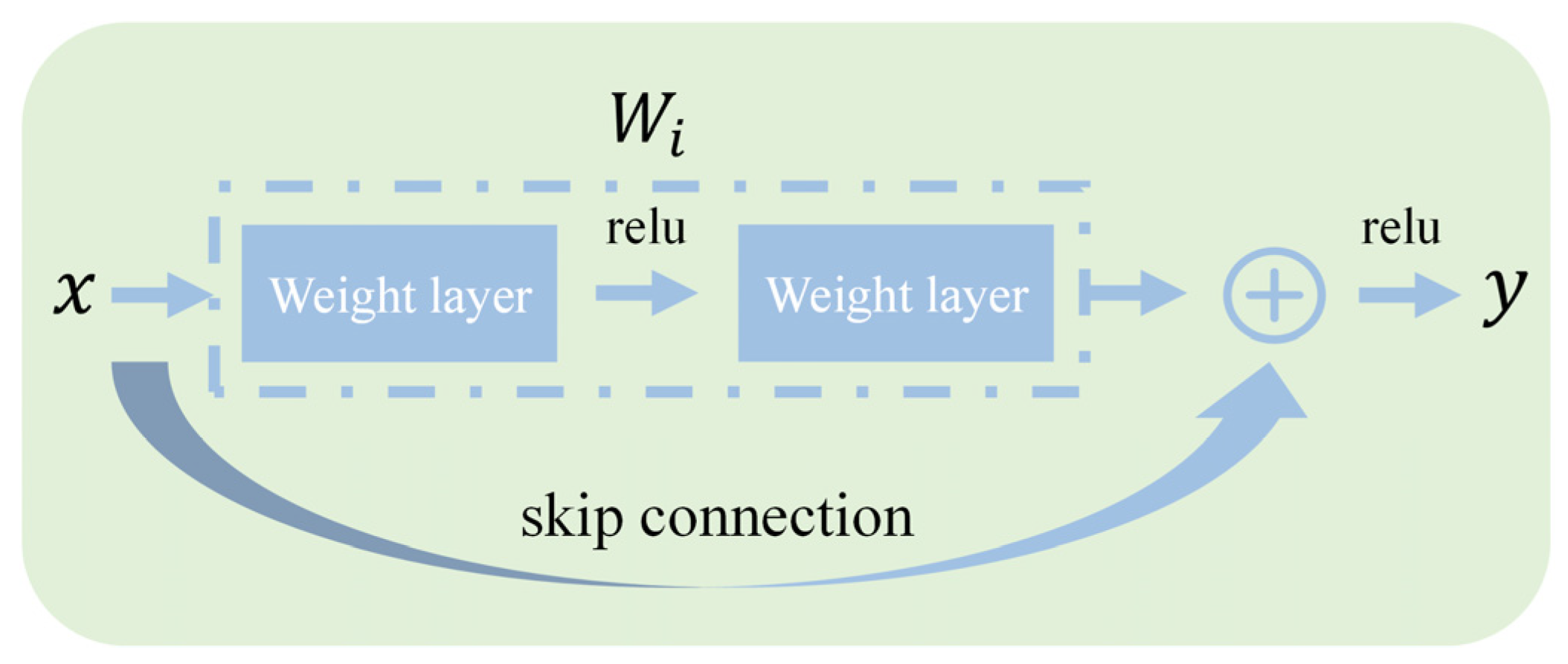However, as the network depth increases, models tend to suffer from issues such as gradient vanishing and network degradation, where training errors no longer decrease but instead increase [38]. To address these problems, He et al. proposed the residual neural network (ResNet), which introduces residual learning and skip connection mechanisms. These innovations significantly improve the training stability and feature representation capacity of deep networks.

The core idea of ResNet lies in the use of identity mappings to directly pass shallow features to deeper layers in the network. As illustrated in the residual connection diagram (Figure 2), the fundamental building block of ResNet is the residual block, which is defined as shown in Equation (7):

$$y=\mathcal{F}\left(x,\left\{W_i\right\}\right)+x,$$

(7)

Here, $x$ represents the input features, $\mathcal{F}$ is the residual function—typically composed of several convolutional layers, batch normalization layers, and activation functions—$W_i$ are the learnable parameters, and $y$ is the output feature.

By adding the original input $x$ to the residual mapping $\mathcal{F}\left(x\right)$, the network is enabled to learn the residual, i.e., the difference between the desired output and the input, rather than attempting to directly model the full mapping. This structure alleviates the problem of gradient attenuation during backpropagation, thereby making it feasible to construct networks with over a hundred layers. In this study, ResNet-18 is selected as the baseline model to balance performance and computational efficiency.

3. Methods

As discussed in the introduction, a single acoustic representation is often insufficient to capture all the discriminative information inherent in complex marine acoustic signals. Time-frequency spectrograms such as the Constant-Q Transform (CQT) and Short-Time Fourier Transform (STFT) offer complementary perspectives of the signal, each with its own advantages in frequency and time resolution, respectively. Their complementarity provides a valuable opportunity to enhance recognition performance. To effectively leverage these two types of features, all models presented in this chapter are built upon a dual-branch residual network (dual-branch ResNet) architecture. This structure includes two independent feature extraction pathways specifically designed for CQT and STFT spectrograms. It allows the network to optimize for the unique characteristics of each feature type, thereby laying a solid foundation for downstream feature fusion.

However, merely extracting features in parallel is not sufficient. The fusion of high-level features from these two independent branches is a critical factor that determines the overall performance of the model—and it is the primary focus of this study. As noted earlier, many existing works rely on simple concatenation strategies, which may fail to fully exploit the synergistic potential of multi-feature integration. Therefore, this chapter systematically introduces and compares several fusion strategies we have explored, aiming to identify more effective approaches for feature integration. The models discussed include the following: 1. A baseline dual-branch ResNet with simple feature concatenation, which serves as a reference point for performance comparison. 2. An attention-driven adaptive fusion network, which explores dynamically learned data-driven weights for feature fusion. 3. The proposed Evaluation-Adaptive Weighted Multi-Head Fusion Network (EAW-MHFN) which represents the final and most advanced architecture in our study.

3.1. Dual-Branch ResNet with Feature Concatenation

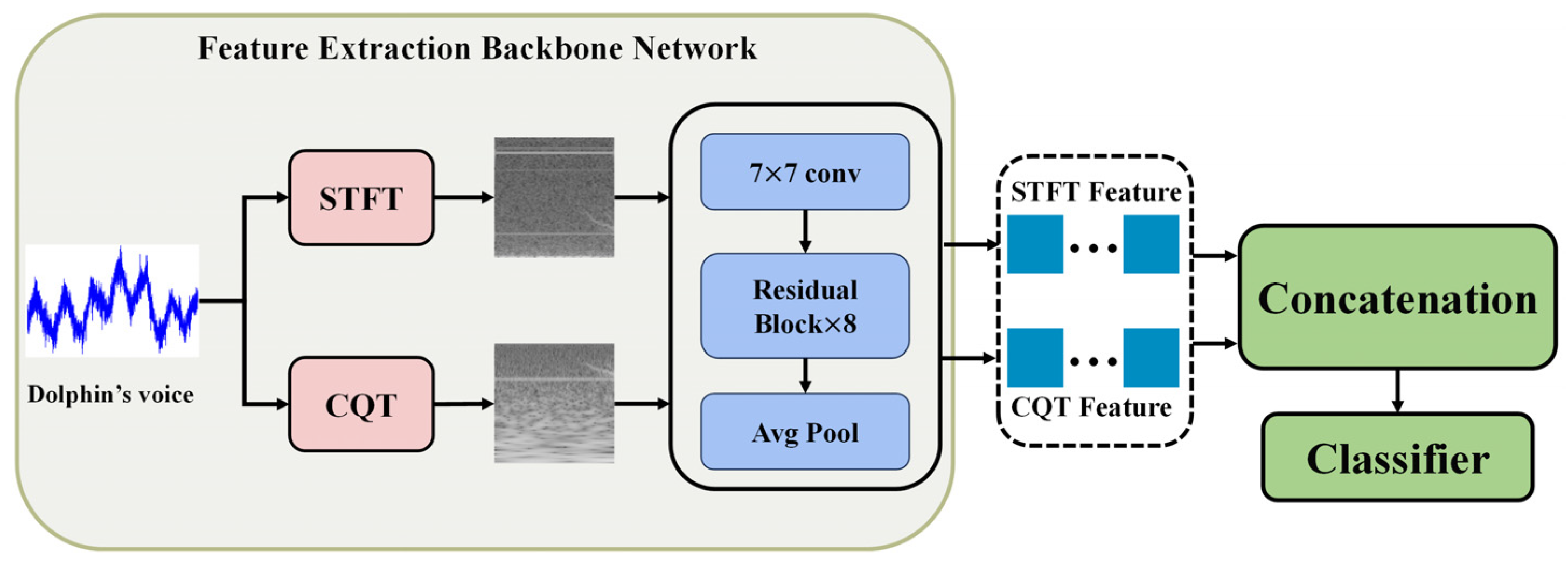
To exploit the modal complementarity between CQT and STFT spectrograms, and to establish a differentiated learning mechanism for heterogeneous features, this study proposes a dual-branch feature fusion architecture based on residual networks. As illustrated in Figure 3, the architecture adopts a parallel feature extraction paradigm, where CQT and STFT inputs are processed through independent forward pathways, followed by hierarchical feature fusion.

Each branch utilizes ResNet-18 with residual learning as the backbone, offering a balanced trade-off between computational efficiency and feature representation capacity. To accommodate single-channel spectrogram inputs, the first convolutional layer in each branch is adapted by modifying the number of input channels from 3 to 1. Furthermore, to preserve the spatial structure of high-level semantic features, the original fully connected classification layer at the end of ResNet is removed and replaced with identity mapping. As a result, each branch outputs a 512-dimensional modality-specific feature vector, denoted as the CQT feature and STFT feature.

During the feature aggregation stage, a simple concatenation-based fusion strategy is adopted to enable interaction between the two branches. Specifically, the 512-dimensional feature vectors from the CQT and STFT branches are concatenated along the channel dimension to form a 1024-dimensional joint feature representation. This strategy provides a good balance between computational cost and information retention, facilitating the capture of cross-modal complementary features.

On top of this feature extraction framework, the baseline model employs a straightforward fusion mechanism. The fused feature vector is passed through a multi-layer perceptron (MLP) for final classification. The classifier consists of a sequential transformation module with the following components:

• A fully connected layer (1024 → 512) followed by batch normalization and ReLU activation;
• A dropout layer with a dropout rate of 0.5;
• A linear projection layer (512 → num_classes).

This design achieves progressive dimensional compression and non-linear transformation, improving classification robustness in complex acoustic environments.

Overall, this model offers a simple yet effective baseline that directly leverages features extracted from dual branches, and serves as a reference point for evaluating more sophisticated fusion strategies introduced later.

3.2. Attention-Driven Adaptive Fusion Network

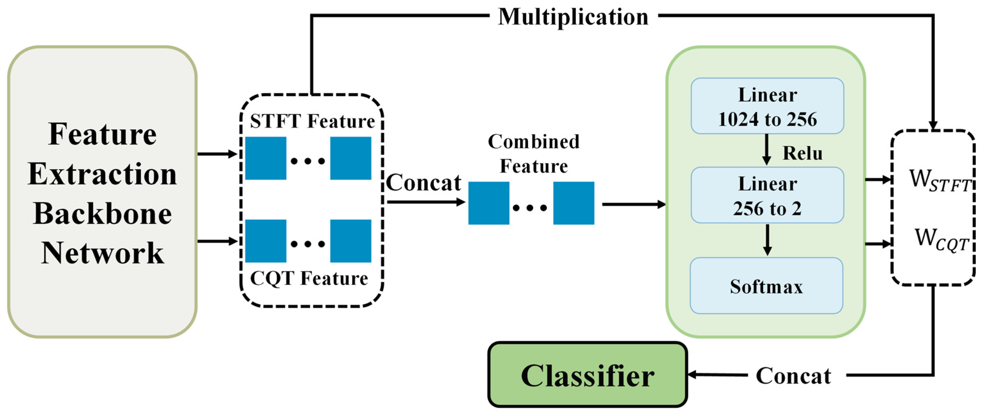
To overcome the limitations of traditional feature concatenation, this study introduces an attention-based adaptive feature fusion method. As illustrated in Figure 4, building upon the dual-branch backbone network described in Section 3.1, we design a cross-modal attention gating module that generates dynamic weighting coefficients through a parameterized mapping network.

The fusion process proceeds as follows:

Given the feature vectors from the two branches—${\mathbf{f}}_c\in {\mathrm{R}}^{512}$ (CQT feature) and ${\mathbf{f}}_s\in {\mathrm{R}}^{512}$ (STFT feature)—we first perform feature concatenation to form a joint representation: ${\mathbf{f}}_{cat}=\left[{\mathbf{f}}_c;{\mathbf{f}}_s\right]\in {\mathrm{R}}^{1024}$.

The concatenated vector is then passed through two fully connected layers to compute adaptive weights, as defined by Equations (8) and (9), where $W_1, W_2$ and $b_1, b_2$ are learnable parameters, and ReLU is the activation function.

$$h_1=ReLU\left(W_1{\mathbf{f}}_{cat}+b_1\right) W_1\in {\mathrm{R}}^{256\times 1024},$$

(8)

$$h_2=W_2{h}_1+b_2 W_2\in {\mathrm{R}}^{2\times 256},$$

(9)

To ensure that the output weights sum to one, i.e., $w_c+w_s=1$, a softmax normalization is applied to $h_2$. The resulting weights reflect the instance-specific importance of the CQT and STFT features.

$$\left[w_c+w_s\right]=Softmax{\displaystyle (}h{\displaystyle )},$$

(10)

These attention weights are then used to recalibrate the feature space via channel-wise multiplication, as shown in Equation (11), where $\odot$ denotes element-wise multiplication.

$${\mathbf{f}}_c^{\mathrm{’}}=w_c\odot {\mathbf{f}}_c,{\mathbf{f}}_s^{\mathrm{’}}=w_s\odot {\mathbf{f}}_s$$

(11)

The final fused representation is then given by ${\mathbf{f}}_{fusion}=\left[{\mathbf{f}}_c;{\mathbf{f}}_s\right]\in {\mathrm{R}}^{1024}$. This formulation not only retains the original information from both modalities but also captures their dynamic interdependence through learned attention. However, it is worth noting that in this model, the attention weights are entirely derived from the current input features through a shallow network, without explicitly leveraging feedback from model performance on the validation set or applying channel-wise enhancement prior to fusion. This observation inspires further investigation into whether more powerful fusion models could be developed by incorporating evaluation-guided supervision or optimized training strategies, potentially leading to superior performance.

3.3. Evaluation-Adaptive Weighted Multi-Head Fusion Network

Building upon the attention-driven adaptive fusion network (ADAFN), we propose the core model of this study—Evaluation-Adaptive Weighted Multi-Head Fusion Network (EAW-MHFN)—to further enhance feature fusion effectiveness and optimize the training process. This model is designed to overcome several potential limitations of ADAFN, including the reliance of attention weights solely on the current input data, the lack of explicit utilization of each branch’s stage-wise performance, and the absence of pre-fusion channel enhancement.

To address these issues, the proposed model incorporates three key mechanisms: intra-branch channel attention (CA), evaluation-based adaptive branch weighting, and multi-head supervised training. Together, these components aim to achieve more intelligent and robust feature fusion and model optimization. As the primary model of this work, EAW-MHFN adopts a more sophisticated fusion strategy and training scheme to further improve feature integration and overall recognition performance. The model remains built upon the dual-branch ResNet18 backbone defined in Section 3.1. Its overall architecture is illustrated in the corresponding Figure 5.

As shown in the figure, after extracting the STFT feature and CQT feature from the feature extraction backbone, the model adopts a multi-head design. Specifically, both 512-dimensional features are not only fed into the subsequent Adaptive Fusion Block, but also passed to two independent auxiliary classifiers. These auxiliary classifiers provide additional supervision signals during training, encouraging each branch to learn more discriminative features effectively.

At the end of each training epoch, the performance (accuracy) of the CQT and STFT branches—denoted as ${ACC}_{CQT}$ and ${ACC}_{STFT}$ respectively—is evaluated on the training set. These evaluation metrics are then used to directly guide the adaptive weighting of branches in the next training phase.

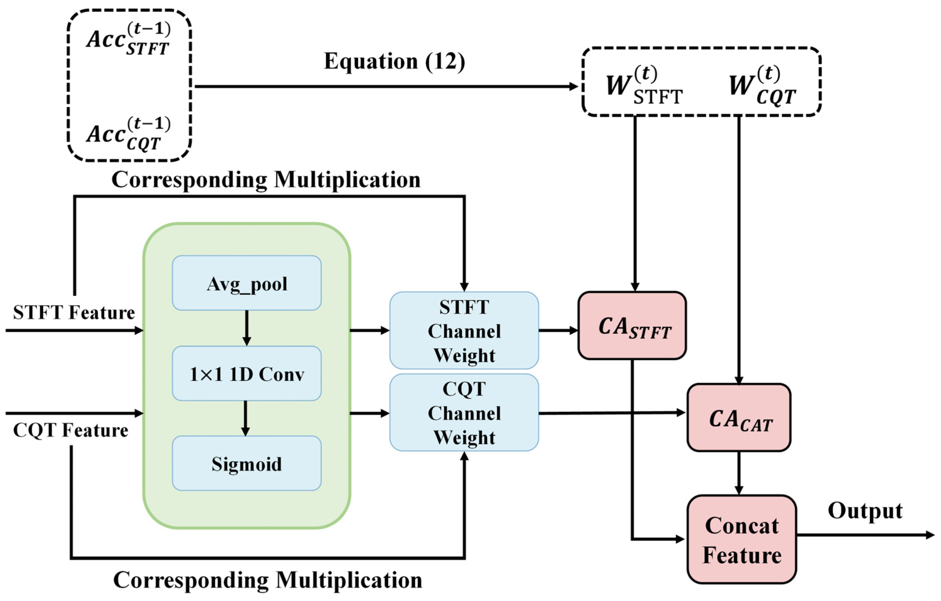
The Adaptive Fusion Block, illustrated in Figure 6, forms the core of this model. It consists of two key components:

• Intra-branch channel attention (CA): Before inter-branch fusion, the CQT feature and STFT feature are first passed through two identical CA modules (as shown in the green boxes in the figure), which include operations such as average pooling, 1×1 1D convolution, and sigmoid activation. These modules learn to adaptively recalibrate the importance of each channel, enhancing informative channels while suppressing redundant or noisy ones. After CA processing, we obtain the channel-refined features: ${CA}_{CQT}$ and ${CA}_{STFT}$.
• Evaluation-based adaptive branch weighting (EBABW): This step dynamically computes the fusion weights for each branch in the current epoch, based on their classification accuracies on the validation set from the previous epoch $\left(t\right)$, based on their classification accuracies on the validation set from the previous epoch ${\displaystyle (}t-1{\displaystyle )}$, denoted as ${ACC}_{CQT}^{{\displaystyle (}t-1{\displaystyle )}}$ and ${ACC}_{STFT}^{{\displaystyle (}t-1{\displaystyle )}}$ As described in Equation (12), these weights are normalized to reflect each branch’s relative contribution. The resulting weights, $W_{CQT}^{{\displaystyle (}t{\displaystyle )}}$ and $W_{STFT}^{{\displaystyle (}t{\displaystyle )}}$, are then applied to the CA-enhanced features ${CA}_{CQT}$ and ${CA}_{STFT}$, respectively. This mechanism ensures that the branch with better performance in previous stages receives more influence during fusion.

$$w_i^{{\displaystyle (}t{\displaystyle )}}={\displaystyle \frac{Ac{c}_i^{{\displaystyle (}t-1{\displaystyle )}}}{Ac{c}_{CQT}^{{\displaystyle (}t-1{\displaystyle )}}+Ac{c}_{STFT}^{{\displaystyle (}t-1{\displaystyle )}}}}$$

(12)

Finally, the two re-weighted feature vectors are concatenated along the feature dimension to form a 1024-dimensional fused feature, which is fed into the final classifier to produce the model’s prediction.

In summary, the EAW-MHFN achieves deep integration of dual-branch features through a carefully designed multi-stage processing pipeline. First, it leverages a multi-head architecture to obtain performance feedback from each branch and provide auxiliary supervision. Then, it applies CA to enhance the internal representations of each branch before fusion. Subsequently, the model dynamically adjusts the fusion weights of each branch based on their historical validation performance, allowing the better-performing branch to have greater influence during integration. This strategy—combining channel attention, performance-driven adaptive weighting, and multi-task learning—is designed to fully exploit the complementary strengths of CQT and STFT features, aiming to achieve superior recognition performance compared to simple concatenation or conventional attention-based fusion methods.

4. Experiment

This chapter presents experiments to validate the effectiveness of the proposed models in the task of marine mammal acoustic recognition. First, we introduce the experimental environment and the preprocessing parameters applied to the audio signals. Section 4.2 describes the evaluation metrics used for assessing model performance. Finally, a series of comparative experiments, ablation studies, and a robustness test are conducted to demonstrate the superiority of the dual-branch fusion architecture, the performance differences among various fusion strategies, and the robustness of each method. In addition, feature visualization is employed to validate the complementarity between CQT and STFT features. For clarity, models are referenced using labels such as Model 3.1, which denotes the dual-branch ResNet feature concatenation model; similarly, Model 3.2 and Model 3.3 refer to the attention-driven adaptive fusion network and the Evaluation-Adaptive Weighted Multi-Head Fusion Network, respectively.

4.1. Experimental Data and Evaluation Metrics

The marine mammal acoustic data used in this study are sourced from the Watkins Marine Mammal Sound Database, an open-access repository established by William Watkins, one of the pioneers in marine mammal bioacoustics. This database comprises recordings spanning nearly seven decades—from the 1940s to the early 21st century—and holds significant historical and scientific value.

The database contains approximately 2000 individual recordings covering over 60 species of marine mammals. The duration of audio samples ranges from 1 s to several minutes, and all files are in wav format.

Table 2. Dataset statistics.

Name	Train	Test	Total
Atlantic Spotted Dolphin	525	212	737
Bottlenose Dolphin	97	39	136
Clymene Dolphin	541	244	785
Common Dolphin	1207	483	1690
Fraser’s Dolphin	1755	735	2490
Grampus Rissos Dolphin	586	239	825
Pantropical Spotted Dolphin	409	152	561
Rough-Toothed Dolphin	220	82	302
Spinner Dolphin	1075	458	1533
Striped Dolphin	470	207	677
White-beaked Dolphin	522	226	748
White-sided Dolphin	624	262	886
Total	8031	3339	11,370

lists the 12 marine mammal species selected for this study, along with the number of samples for each category [33].

Due to the diversity in both duration and sampling rates among the audio files, all data were standardized by segmenting each audio clip into multiple 200 ms segments and resampling them to a common sampling rate of 30,000 Hz, based on the shortest and lowest-quality original audio file. This preprocessing step increased the amount of training data and enhanced the classification accuracy. The dataset was split into a training set and a testing set at a ratio of 7:3. To ensure the validity of the evaluation, segments derived from the same original audio file were not allowed to appear in both training and testing sets simultaneously. The experimental environment is configured as follows: image size: 224 × 224, batch size: 32, epochs: 30, GPU: NVIDIA GeForce RTX 2060, CPU: AMD Ryzen 7 4800H, RAM: 16 GB, framework: PyTorch (version 2.1.1), CUDA version: 12.1.

$$Accuracy={\displaystyle \frac{TP+TN}{TP+TN+FP+FN}}$$

(13)

$$Precision={\displaystyle \frac{TP}{TP+FP}}$$

(14)

$$Recall={\displaystyle \frac{TP}{TP+FN}}$$

(15)

$$F1-score={\displaystyle \frac{2\times Precision\times Recall}{Precision+Recall}}$$

(16)

To evaluate the classification performance, several standard metrics were employed, including Accuracy, Precision, Recall, and F1-Score. These metrics provide a comprehensive view of the model’s predictive quality: Accuracy measures the proportion of correctly predicted samples over the total number of samples (Equation (13)). Precision refers to the ratio of correctly predicted positive samples to all samples predicted as positive (Equation (14)). Recall denotes the ratio of correctly predicted positive samples to all actual positive samples (Equation (15)). F1-Score is the harmonic mean of Precision and Recall, offering a balanced evaluation of the model’s performance (Equation (16)).

The meanings of TP, TN, FP, and FN in the above four formulas are shown in

Table 3. Comparison table of TP, TN, FP, and FN.

Abbreviation	Full Form	Meaning
TP	True positive	Correctly detected positive results
TN	True negative	Correctly detected negative results
FP	False positive	Incorrectly detected positive results
FN	False negative	Incorrectly detected negative results

.

Because these concepts can be confusing, this paper further explains through an example. Suppose we have 100 samples: 60 positive samples and 40 negative samples. If the system finds 50 samples, of which only 40 are true positive samples, we can calculate the above metrics.

TP: The number of positive samples predicted as positive samples is 40; FN: The number of positive samples predicted as negative samples is 20; FP: The number of negative samples predicted as positive samples is 10; TN: The number of negative samples predicted as negative samples is 30.

To evaluate the efficiency of the proposed models, we measured their computational cost using three key metrics:

Parameters: This is a static metric that depends solely on the model architecture. It measures the total size of all “learnable” components in the model. The parameter count is calculated entirely based on the defined model structure, independent of input data size, hardware performance, or any other external factors. It includes all layers with learnable weights and biases, specifically convolutional layers (Conv2d), fully connected layers (Linear Layers), and batch normalization layers (BatchNorm). Layers such as activation functions (ReLU), pooling layers (Pooling), and dropout layers (Dropout) do not contain learnable parameters, so their parameter count is zero.

FLOPs: This is a semi-dynamic metric that depends on both the model structure and input size. It calculates how many mathematical operations are required for the model to make a single prediction. FLOPs vary with input size even for the same model—for example, a 224 × 224 image versus a 416 × 416 image (this paper uses 224 × 224 inputs) results in different FLOPs. It measures the total number of floating-point operations (additions, subtractions, multiplications, divisions) needed for one forward pass. The most significant contributor to this metric is the convolutional layers, i.e., the Feature Extraction Backbone Network.

Inference time: This refers to the actual time it takes for the model to complete a single forward pass on a specific hardware platform. It is a practical metric that directly reflects the model’s real-world running speed and is heavily influenced by hardware performance—more powerful hardware can significantly reduce inference time. In this paper, the inference time is measured as the time to process a single input on the given hardware. To ensure data reliability, the process is repeated 100 times, and the average is taken as the final inference time.

4.2. Baseline Performance Comparison

In this section, we conduct a baseline comparison experiment to verify the performance advantage of the fusion-based model design. Specifically, we compare a single-branch ResNet model (abbreviated as ResNet in the table) with Model 3.1, which adopts a dual-branch feature concatenation strategy. The experimental results are shown in

Table 4. Comparison Results Between ResNet and Model 3.1.

Input	Model	Accuracy	Precision	Recall	F1-Score
CQT	ResNet	61.43	63.06	61.42	61.28
STFT	ResNet	94.37	94.87	94.37	94.39
CQT + STFT	Model 3.1	94.76	95.08	94.76	94.77

.

The single-branch model is based on ResNet18, with the original classification head replaced by the same classifier used in Section 3.1, to ensure a fair and rigorous comparison. From the results, it can be observed that the dual-branch model significantly outperforms the single-branch model when using CQT features. However, compared to the STFT feature-based model, the performance gain is marginal, with accuracy improving by only 0.39%.

Table 4 and

Table 5. Computational cost comparison between ResNet and Model 3.1.

Model	Parameter(M)	FLOPs(G)	Inference Time(ms)
ResNet	11.31	3.49	3.74
Model 3.1	22.87	6.98	7.00

show that the dual-branch architecture leveraging complementary features is indeed effective. However, the dual-branch model contains 22.87 million parameters, nearly twice the 11.31 million parameters of the single-branch model. The same applies to the other two parameter metrics. Given the significant increase in model complexity, the slight performance improvement suggests an inefficiency in parameter utilization.

Therefore, the subsequent research in this paper focuses on exploring more efficient fusion methods for combining dual-branch features.

4.3. Comparison of Fusion Strategies

This section investigates the impact of different fusion strategies on recognition performance. Compared with simple feature concatenation, the models described in Section 3.2 and Section 3.3 adopt more sophisticated architectural designs and learning strategies. Notably, however, these models do not significantly increase the number of parameters.

Table 6. Performance comparison of Models 3.1, 3.2, and 3.3.

Model	Accuracy	Precision	Recall	F1-Score
Model 3.1	94.76	95.08	94.76	94.77
Model 3.2	95.15	95.28	95.15	95.16
Model 3.3	96.05	96.21	96.05	96.02

and

Table 7. Computational cost comparison between Models 3.1, 3.2, and 3.3.

Model	Parameter(M)	FLOPs(G)	Inference Time(ms)
Model 3.1	22.87	6.98	7.00
Model 3.2	23.13	6.98	7.64
Model 3.3	23.14	6.98	7.77

compare the three dual-branch models proposed in Chapter 3. From the results, it is evident that dynamically adjusting feature vectors leads to better performance in recognition tasks than naive concatenation.

Among the three models, Model 3.3 achieves the best overall performance, reaching an accuracy of 96.05%. Compared to Model 3.1, Model 3.2 enhances recognition performance by introducing a dynamic feature weighting module. However, this module generates weights through relatively simple connections within the network, which limits its ability to accurately assess the relative importance of CQT and STFT features. In contrast, Model 3.3 combines channel attention mechanisms and historical performance-based dynamic weighting, which enables a richer and more robust estimation of feature importance for both CQT and STFT inputs. As a result, the recognition performance of the model in Section 3.3 is significantly improved. Moreover, the computational complexity difference among the three models is minimal, which means that in practical scenarios, Model 3.3 does not impose additional hardware requirements.

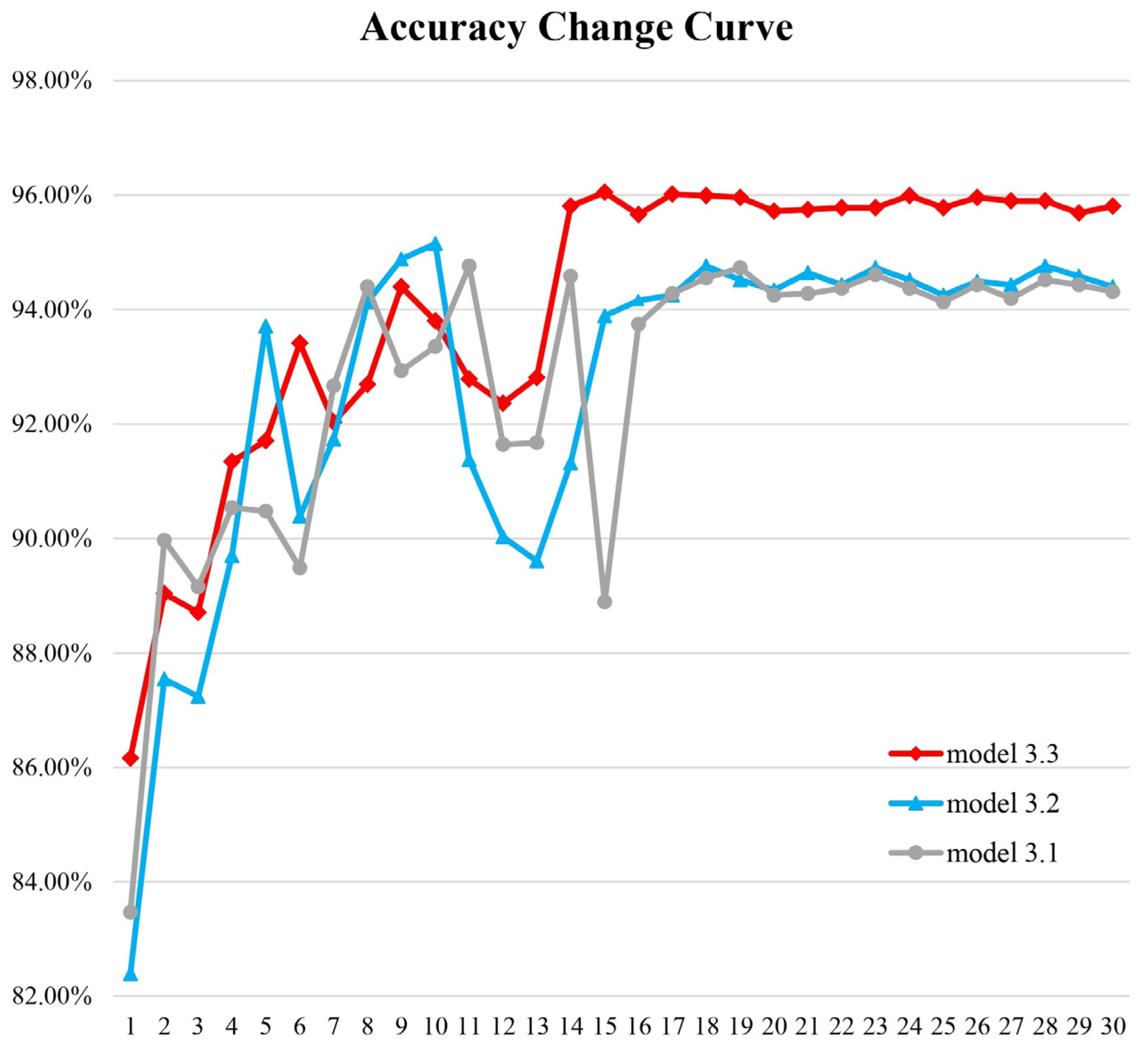
To further examine the training process of these models, accuracy curves were plotted as shown in Figure 7. It can be observed that during the early stages of training, all three models exhibit considerable fluctuations in accuracy. However, Model 3.3 shows significantly smaller fluctuations compared to the other two. As training progresses, all models eventually converge. Once convergence is reached, Model 3.3 clearly outperforms Models 3.1 and 3.2, while Model 3.2 achieves a slight advantage over Model 3.1.

To better observe the training curve of Model 3.3, Figure 8 presents the changes in training accuracy and test accuracy over time. As shown in the figure, the test accuracy closely follows the trend of the training accuracy, with only a small difference between the two. Moreover, when the training accuracy nearly reaches 100%, the test accuracy also peaks at 96.05%. This demonstrates that the model has been thoroughly trained.

4.4. Ablation Study of Model 3.3

The Adaptive Fusion Block in Model 3.3 integrates two distinct weighting strategies: channel attention weighting and evaluation-based adaptive branch (EBAB) weighting. To better understand the individual impact of each strategy on the recognition performance, an ablation study was conducted.

First, we evaluated the classification ability of the baseline model, i.e., Model 3.1, which does not include the CA module or the EBAB module.

Next, we retained the channel attention (CA) module, but removed the accuracy-based weights $W_{CQT}^{{\displaystyle (}t{\displaystyle )}}$ and $W_{STFT}^{{\displaystyle (}t{\displaystyle )}}$, meaning the CA-enhanced features were not further re-weighted by the evaluation-driven scores.

Then, we removed the CA module and directly applied the evaluation-based weights $W_{CQT}^{{\displaystyle (}t{\displaystyle )}}$ and $W_{STFT}^{{\displaystyle (}t{\displaystyle )}}$ to the raw CQT and STFT features to generate the fused representation.

Finally, both modules were used together, forming CA + EBAB.

The experimental results are shown in Figure 9. As the data reveal, neither strategy alone significantly outperforms the other, and both yield performance lower than Model 3.2’s 95.15% accuracy. However, when both strategies are used in conjunction, the model is better able to identify and emphasize critical features, leading to superior overall recognition performance.

4.5. Feature Visualization Analysis

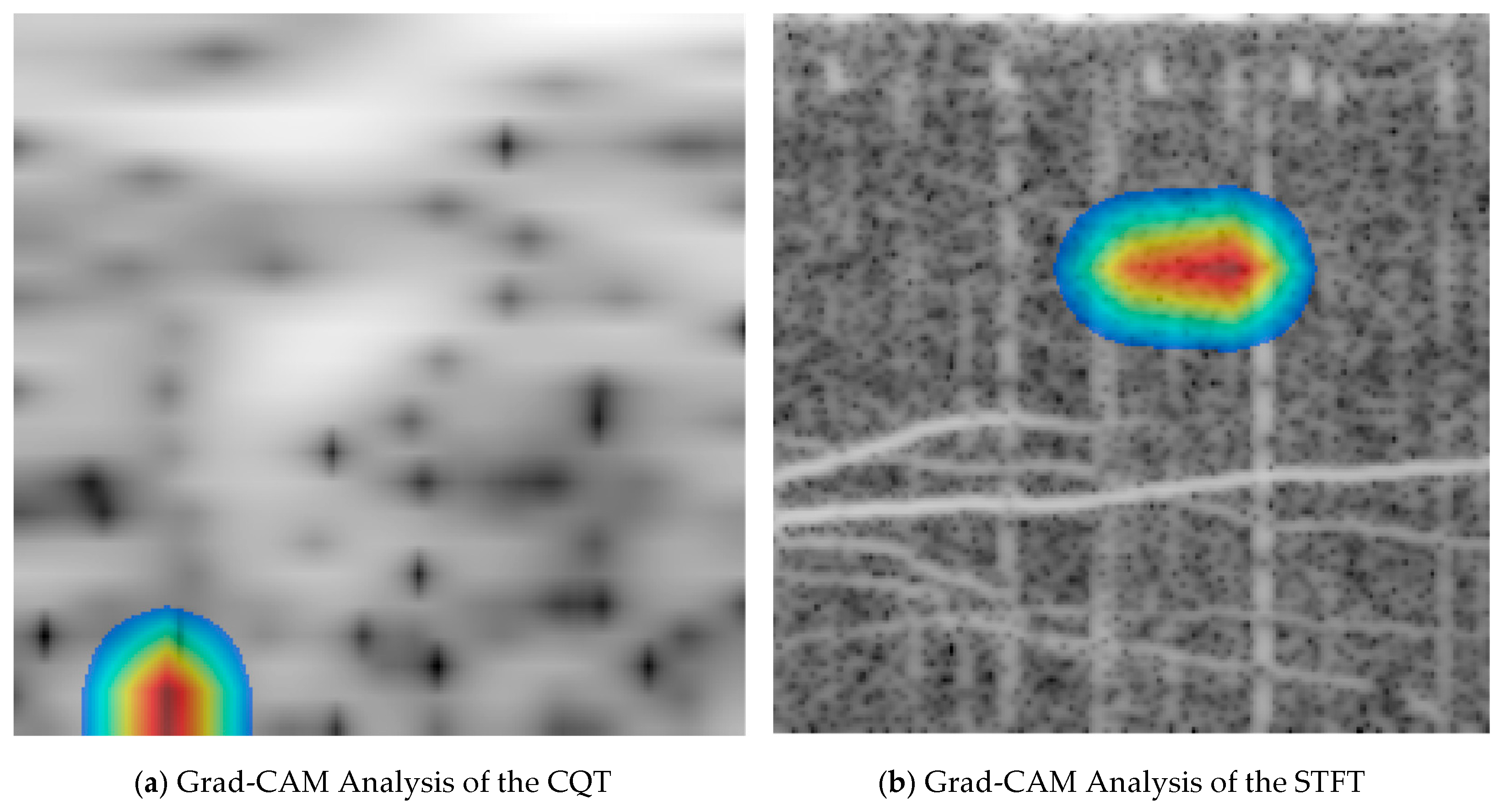
To observe the regions of interest in Model 3.3, we used Grad-CAM to generate heatmaps, as shown in Figure 10. Figure 10a is the CQT feature map computed from the WAV file, and Figure 10b is the STFT feature map computed from the same WAV file.

It can be seen that for the CQT features, the model focuses more on the low-frequency regions where the frequency resolution is higher. In contrast, for the STFT features, the model pays more attention to the line spectra in the mid-to-high frequency regions. This further confirms the complementary nature of CQT and STFT features.

4.6. Robustness Evaluation of Model 3.3

To further evaluate the generalization and robustness of the proposed fusion strategy when applied to other types of features, Mel-spectrogram features [39] were introduced into the experiment. Different combinations of input features were tested with both Model 3.2 and Model 3.3. Specifically, the combinations excluded single-feature inputs and covered the following four multi-feature scenarios: CQT + STFT, CQT + Mel, STFT + Mel, and CQT + STFT + Mel.

For the three-feature combination, the architecture was extended into a three-branch structure based on the same backbone as previous models. Since the essential components of the model remained unchanged aside from minor adjustments in input/output dimensions, the detailed architecture is omitted for brevity.

The experimental results for each input configuration are presented in

Table 8. Robustness test results of Models 3.2 and 3.3.

Feature	Model	Accuracy
CQT	ResNet	61.43
STFT		94.37
Mel		91.73
CQT + STFT	Model 3.2	95.15
	Model 3.3	96.05
CQT + Mel	Model 3.2	92.81
	Model 3.3	93.29
STFT + Mel	Model 3.2	94.79
	Model 3.3	94.70
CQT + STFT + Mel	Model 3.2	94.49
	Model 3.3	95.60

.

As shown in Table 8, compared to using a single type of feature, both dual-feature and triple-feature combinations significantly enhance the model’s recognition performance. However, the inclusion of all three features introduces excessive redundancy, resulting in an accuracy that does not surpass the CQT + STFT combination. This further confirms the superior complementarity between CQT and STFT features in the context of this acoustic recognition task.

5. Conclusions

To improve marine mammal acoustic recognition, this study proposes the Evaluation-Adaptive Weighted Multi-Head Fusion Network (EAW-MHFN), which integrates CQT and STFT features using a dual-branch ResNet. The proposed model achieved a state-of-the-art accuracy of 96.05% on the Watkins marine mammal sound dataset, significantly outperforming single-feature and other fusion-based models.

The model’s success stems from two key innovations: intra-branch channel attention (CA) for feature enhancement, and a novel evaluation-based adaptive weighting mechanism that dynamically adjusts each branch’s influence based on its historical validation accuracy. Ablation studies confirmed the critical synergy of these components.

Our findings demonstrate that the fusion strategy is as crucial as the features themselves. The EAW-MHFN provides a robust and effective solution for complex bioacoustic classification, offering significant practical value for automated marine wildlife monitoring and ecological conservation.

However, this study’s conclusions are based on a specific dataset, which naturally defines the scope for future work. A key priority will be to test the model’s robustness under controlled Signal-to-Noise Ratios (SNRs) and its effectiveness in multi-label scenarios with overlapping calls. Furthermore, expanding the dataset to a wider range of marine mammal species is a critical step to test generalization. We are particularly optimistic about this direction, as we expect the distinct frequency characteristics between species to highlight the complementary strengths of our CQT/STFT fusion. Conversely, a more ambitious challenge lies in fine-grained, individual-level identification, where the high similarity of intra-species vocalizations would likely require novel feature representations. Finally, while this study validates a 2D feature fusion approach, exploring the integration of other feature types (e.g., MFCCs) via multi-modal architectures remains a promising research avenue.