Prediction of Target-Induced Multipath Interference Acoustic Fields in Shallow-Sea Ideal Waveguides and Statistical Characteristics of Waveguide Invariants

Abstract

The acoustic scattering of targets in shallow-sea waveguides exhibits complex features such as multipath propagation and intricate echo components, with its acoustic field properties remaining incompletely understood. This study employs a hybrid method combining normal modes and scattering functions to numerically model the acoustic scattering of targets in waveguide channels. We analyze the coupling mechanisms of multipath acoustic waves and derive precise predictive formulas for the bright–dark interference fringe patterns in range–frequency spectra based on the physical mechanisms governing acoustic field interference. By tracking the peak trajectories of these interference fringes in range–frequency spectra, we investigate the variations of the waveguide invariant with frequency, range, and depth, revealing statistical patterns of the waveguide invariant in target–waveguide coupled scattering fields under different water depths. The results demonstrate that, under constant channel conditions, waveguide properties exhibit a weak correlation with target material characteristics. In shallow water environments, waveguide invariant values display broader distributions with higher probability density peaks, whereas increasing water depth progressively narrows the distribution range and monotonically reduces the peak magnitudes of the probability density function. Experimental validation via scaled elastic target echo testing confirms the observed trends of waveguide invariant variation with water depth.

1. Introduction

In ocean waveguides, the acoustic scattering of targets involves complex physical processes such as reflection, transmission, resonant excitation, and reradiation. These processes, coupled with interactions between the sound source and waveguide environment, lead to intricate variations in the scattered acoustic field [1,2]. In 1982, Chuprov investigated the interference characteristics of ocean waveguide fields in the spatial frequency domain and introduced the concept of the waveguide invariant, which is denoted by β, establishing a theoretical foundation for analyzing acoustic interference patterns [3]. Building on this theory, researchers have developed diverse methodologies and applications. For instance, Su [4] proposed a frequency shift compensation method based on β to enhance horizontal–longitudinal coherence in acoustic fields. Zurk et al. validated the invariance principle for active sonar through tank experiments, extracting β from spectrograms using Hough transforms [5]. Zhu [6] explored the interference features of acoustic vector fields in the frequency–range domain for shallow Pekeris waveguides, analyzing the formation mechanisms of interference structures in sound intensity spectra, particle velocity autospectra, complex intensity spectra, and wave impedance spectra, and discussed the role of β in characterizing these structures. Lu [7] simplified the time–frequency analysis of waveguide signals via warping transforms, enabling dispersion curve extraction with only prior knowledge of the β’s range. Yao [8] estimated β by leveraging the proportional relationship between line spectral intensity fluctuations and their scaled counterparts in low-frequency recorded spectrograms. Mo [9] employed line detection algorithms to extract interference patterns from vector acoustic fields for β estimation. Li [10,11] advanced beamforming-based simulations using array-received signals to extract β without requiring environmental parameters.

In source localization and depth estimation, Liu [12] developed a method to discriminate source depths using β, demonstrating distinct invariant values for surface and submerged sources when receivers are deployed below negative thermoclines. Wang [13] introduced a broadband source depth discrimination approach for deep-sea environments, correlating frequency-dependent interference structures in deep-sea acoustic fields with those in vertical line array beamforming outputs and deriving expressions for broadband beamformed fields. Dun [14] proposed a deep-water moving target detection and localization method utilizing multipath Doppler effects and wideband ambiguity functions (WAFs), effectively separating target echoes from reverberation in complex environments. Xu [15] devised a broadband near-surface source depth estimation method based on frequency domain interference features in deep-sea bottom reflection zones. In waveguide parameter inversion, Li [16] introduced a Bayesian theory-based approach for ocean parameter inversion using single-hydrophone dispersion curves, aligning with Zhai’s [17] source localization method based on frequency–notch matching of interference structures.

In the domain of complex waveguide modeling, Zakharenko [18] proposed a perturbation formulation based on Taylor series expansion, deriving analytical expressions for the first- to third-order derivatives of modal horizontal wavenumbers and eigenfunctions under varying water depths. By integrating these results with a wide-angle parabolic equation (PE) model, they established an efficient acoustic field computation framework validated in a three-dimensional coastal wedge-shaped waveguide through single-mode perturbation expansion. Subsequently, Kozitski [19] advanced an elastic seabed coupling model, employing a multi-scale expansion method to construct coupled-mode parabolic equations for weakly elastic seabeds. This approach circumvented the direct computation of elastic modes and achieved high consistency with the source image method in the ASA wedge benchmark problem with shear wave velocities below 300 m/s. In contrast, Su [20] experimentally observed anomalous interference fringe patterns in shallow-water low-frequency acoustic fields, revealing contradictions between high waveguide invariant values (β ≈ 1.03) and single-mode dominance below 150 Hz, phenomena that are unexplainable by conventional fluid seabed models. To resolve this, they proposed a two-layer seabed model incorporating an elastic basement, inverting geoacoustic parameters of the sediment layer and basement through spatial coherence analysis of acoustic fields. Their work demonstrated significant suppression of low-frequency modal amplitudes caused by leakage attenuation induced by the elastic basement. Furthermore, Mei [21] introduced an innovative β-S Dimensional Assignment (β-SDA) method, employing warping transforms to extract range-dependent spectral features and constructing a joint confidence-based association cost function. The β-SDA method effectively mitigates false target proliferation in traditional bearing-only localization systems caused by low detection rates.

Although numerous advanced techniques currently exist for extracting interference fringes, explanations of their underlying causes and mechanisms remain incomplete, and comparative studies on fringe fitting are insufficient. Previous investigations of waveguide invariants in shallow-sea environments predominantly rely on range values calculated from a limited number of extracted interference fringes using existing methods, failing to comprehensively elucidate their statistical characteristics under given test conditions. To address these limitations, this study introduces the following advancements: (1) Model development: A numerical model for acoustic scattering from targets in idealized shallow-sea waveguide channels is constructed. By integrating normal mode theory with target scattering functions, range–frequency spectra of targets at varying depths are computed, explicitly explaining the physical mechanisms responsible for the generation of bright–dark alternating interference fringe patterns. (2) Analytical derivation: Based on the physical principles governing multipath acoustic wave interactions in waveguides, ray paths from the source to the receiver are rigorously described. Analytical formulas for interference spectral peaks as functions of frequency and range are derived, thereby validating the interference mechanisms and characteristics observed in numerical solutions. (3) Based on the extracted interference fringe peaks, the waveguide invariant was calculated, and its statistical properties were derived to investigate whether the waveguide invariant can be utilized to determine the depth of scattering objects. The corresponding conclusions were experimentally validated.

2. Acoustic Scattering by Targets in Ideal Acoustic Waveguides

When considering an ideal ocean waveguide, the sound speed and density of the water layer are assumed to be homogeneous and constant. As illustrated in Figure 1, the water depth is H. A coordinate system is established with the origin O defined at the sea surface directly above the center of the transmitter. The z-axis is oriented positive vertically downward, and the x-axis is positive horizontally to the right. The distance from the transmitter to the receiver is denoted as r₁, while the distance from the target to the receiver is r₂. The source depth is z_s, the target depth is z_t, and the receiver depth is z_r.

The sound pressure field at the receiver is the linear superposition of the incident acoustic field from the transmitter and the scattered acoustic field from the target. For the idealized ocean waveguide model, the water column is assumed to be a constant sound speed layer, with the sea surface modeled as a pressure release boundary and the seafloor as a perfectly rigid boundary. To focus on analyzing the dominant horizontal propagation modes in shallow-water waveguides, the system adopts a simplified collinear source-receiver-target geometry for effective statistical analysis of multipath interference. Based on normal mode theory, the backscattered acoustic field from the target in an ideal waveguide environment is derived as [22,23,24]:

$$p\left(r_1,z_t,r_2,z_r,z_s,f\right)=C^2\sum _m\sum _n{\psi }_m\left(z_s\right){\psi }_m\left(z_t\right){\displaystyle \frac{e^{i{k}_{rm}{r}_1}}{\sqrt{k_{rm}{r}_1}}}S\left({\theta }_m,\varphi ;{\theta }_n,{\varphi }_0\right){\psi }_n\left(z_t\right){\psi }_n\left(z_r\right){\displaystyle \frac{e^{i{k}_{rn}{r}_2}}{\sqrt{k_{rn}{r}_2}}}$$

(1)

The constant C is defined as follows:

$$C={\displaystyle \frac{i{e}^{\frac{-i\pi }{4}}}{\rho \sqrt{8\pi }}}$$

(2)

$S\left({\theta }_m,\varphi ;{\theta }_n,{\varphi }_0\right)$ is the scattering function, m and n are mode numbers, k_rm and k_rn denote horizontal wavenumbers, k_zm and k_zn denote vertical wavenumbers, and ${\psi }_m$ represents the following mode function:

$${\psi }_m\left(z\right)=Asin\left(k_{zm}z\right)+Bcos\left(k_{zm}z\right)$$

(3)

where A and B are undetermined coefficients. Due to the pressure release boundary condition at the surface, B = 0.

The vertical wavenumber k_zm is given by the following:

$$k_{zm}H=\left(m-{\displaystyle \frac{1}{2}}\right)\pi ,\mathrm{m}=\mathrm{1,2}\dots ,$$

(4)

The horizontal wavenumber k_rm is expressed as follows:

$$k_{rm}=\sqrt{{\left({\displaystyle \frac{2\pi f}{c}}\right)}^2-{\left[\left(m-{\displaystyle \frac{1}{2}}\right){\displaystyle \frac{\pi }{H}}\right]}^2},m=\mathrm{1,2},\dots$$

(5)

Both k_zn and k_rn are computed identically. In practical waveguides, the propagation modes are approximately horizontal ($\theta =0$). By substituting Equation (2) into Equation (1), the following expression is derived:

$$p\left(r_1,z_t,r_2,z_r,z_s,f\right)=C^2\sum _m\sum _n\sin \left(k_{zm}{z}_s\right)\sin \left(k_{zm}{z}_t\right){\displaystyle \frac{e^{i{k}_{rm}{r}_1}}{\sqrt{k_{rm}{r}_1}}}S\left(0,\varphi ;0,{\varphi }_0\right)\sin \left(k_{zn}{z}_r\right)\sin \left(k_{zn}{z}_t\right){\displaystyle \frac{e^{i{k}_{rn}{r}_2}}{\sqrt{k_{rn}{r}_2}}}$$

(6)

Once the scattering function of the target is determined, the acoustic scattering characteristics of the target in the ocean waveguide can be computed using Equation (6).

3. Numerical Simulation of Scattered Acoustic Fields

3.1. Numerical Simulation Model and Parameters

To investigate the scattering properties of diverse targets in waveguides, standard spherical models with two material configurations (rigid models and elastic models incorporating stainless steel parameters) are selected as illustrative examples.

Table 1. Acoustic parameters for the numerical computational model.

	Dimension/m	Density/kg·m−3	Longitudinal Wave Speed/m·s−1	Shear Wave Speed/m·s−1
Water	Depth 100	1000	1500	-
Rigid Sphere	Radius 5	-	-	-
Elastic Sphere	Radius 5	7900	6420	3040

summarizes the acoustic and material parameters required for modeling.

The oceanic waveguide is configured as an ideal environment with a water depth of 100 m and a uniform sound speed of 1500 m/s. The source, receiver, and target are collocated at the same depth, consistent with the schematic diagram shown in Figure 1. The source signal operates within the frequency band of 1000–2000 Hz, and the modal summation is truncated at 40 modes.

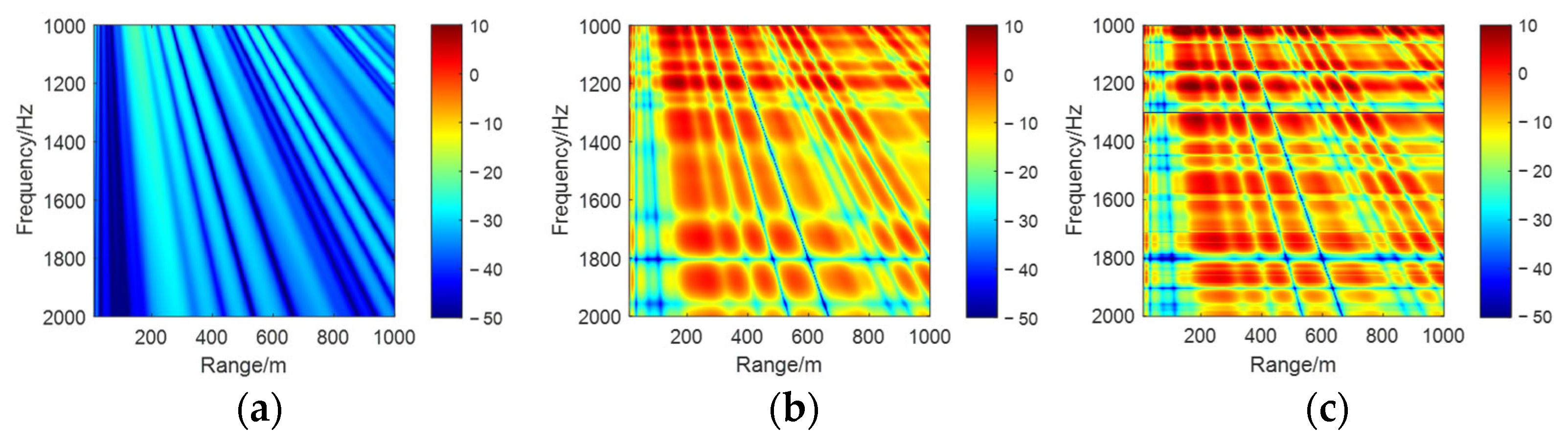
3.2. Numerical Simulation of Range–Frequency Spectra

Under ideal waveguide conditions, the backscattered sound pressure levels from rigid and elastic spheres were computed as functions of receiver position and frequency at source and target depths of 30 m, 50 m, and 60 m, with the corresponding range–frequency spectrograms presented in Figure 2, Figure 3 and Figure 4, where subplots (a), (b), and (c) in each figure, respectively, represent the channel sound field without a target, the scattered field with a rigid target, and the scattered field with an elastic target.

As shown in Figure 2, Figure 3 and Figure 4, the backscattered range–frequency spectrograms of the channel background, rigid sphere, and elastic sphere exhibit two distinct types of interference fringes under identical target depths, collectively forming the spectral interference structures. The downward-sloping linear fringes demonstrate consistent slope trends across different targets at the same depth, which correlate with the multipath characteristics inherent to the waveguide. In the ideal waveguide, the acoustic field at the receiver arises from the superposition of the direct wave from the source, the specular reflected echo from the target, and the sea surface and seafloor reflected waves, generating the multipath interference phenomena typical of ocean waveguides. Additionally, horizontally oriented resonant peaks emerge due to the interaction of Franz waves [25,26,27]—a type of diffracted wave propagating along the sphere’s surface—with specular reflections. These interactions induce narrowband transverse bright–dark fringes in the range–frequency spectrum. For elastic targets, material and structural properties further excite whispering gallery waves [27] in addition to Franz waves, leading to more intricate scattering behavior compared to rigid spheres. Consequently, the resonant peaks of elastic targets exhibit richer variations in transverse fringe patterns, characterized by additional spectral peaks and enhanced modulation. This complexity underscores the influence of target elasticity on waveguide-coupled scattering dynamics, offering distinct spectral signatures for material discrimination in inverse scattering applications.

Furthermore, our analysis reveals that the fundamental morphology of interference fringes is strongly correlated with the target depth and horizontal displacement. Under conditions of fixed target depth and identical horizontal displacement of the receiving transducer, the slope trends of the oblique interference fringes remain consistent across targets of different materials. This indicates a weak correlation between the fringe slope and target material properties under such configurations. However, material differences—particularly between elastic and rigid targets—significantly influence the transverse intensity modulation and fine structural details of resonance fringes.

4. Mechanisms and Interference Fringe Prediction of Target-Induced Acoustic Scattering with Multipath Coupling

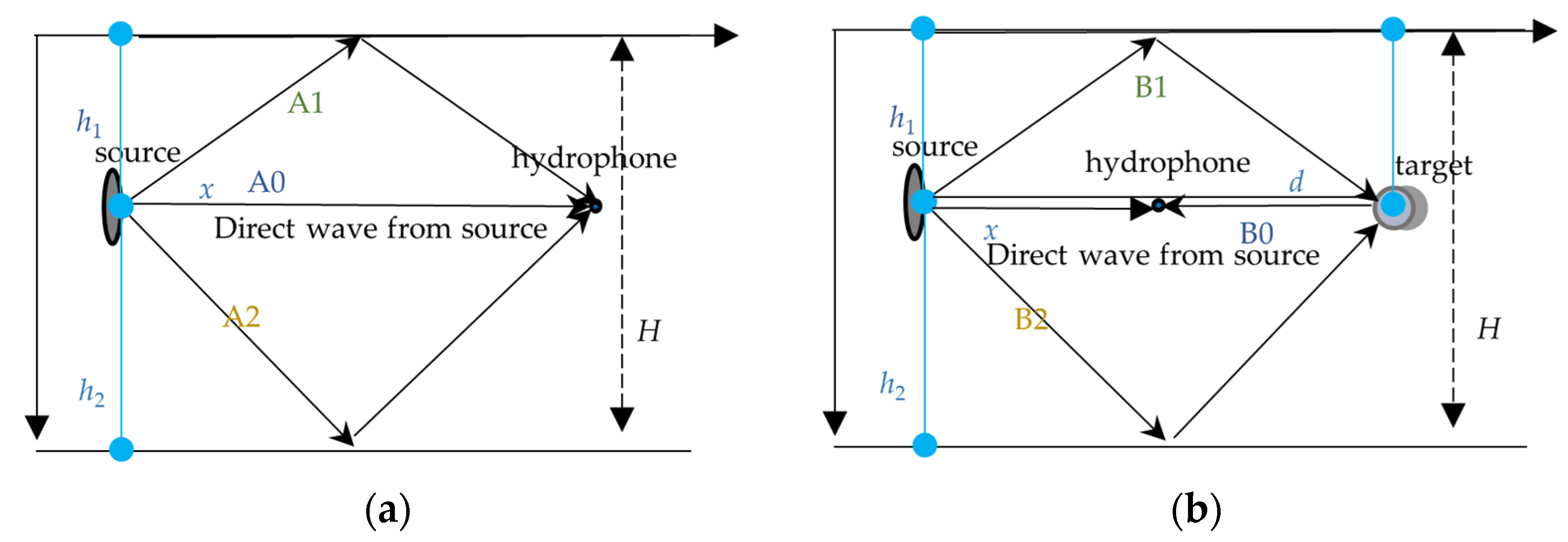
4.1. Mechanisms of Target-Induced Acoustic Scattering with Multipath Coupling

In the configuration depicted in Figure 5, the transmitter, receiver, and target are collocated at the same depth. The direct wave path length to the receiver is defined as x, the water depth is denoted as H, and the source is positioned at depths h₁ below the sea surface and h₂ above the seafloor. The separation distance between the source and target is d.

Under the influence of the waveguide, the acoustic wave propagation paths are categorized into distinct components based on boundary interactions and target coupling. For the baseline waveguide without a target, the primary sound paths include three distinct propagation paths, as illustrated in Figure 5a. When incorporating target–waveguide coupling, the propagation paths further involve scattering at the target, comprising four scattering paths, as depicted in Figure 5b. The geometric lengths of these paths, critical for phase coherence analysis in interference patterns, are systematically quantified in

Table 2. Acoustic wave components and their propagation paths.

ID	Wave Type	Propagation Path/m
A0	Direct Wave From Source	x
A1	Source → Sea Surface → Hydrophone	$\sqrt{(2{\ast h_1)}^2+x^2}$
A2	Source → Seafloor → Hydrophone	$\sqrt{(2\ast {h_2)}^2+x^2}$
B0	Source → Target → Hydrophone	$2d-x$
B1	Source → Sea Surface → Target → Hydrophone	$\sqrt{(2\ast {h_1)}^2+d^2}+d-x$
B2	Source → Seafloor → Target →Hydrophone	$\sqrt{(2\ast {h_2)}^2+d^2}+d-x$

.

4.2. Interference Fringe Prediction Equation

As indicated in Table 2, the oblique fringe peaks observed in the spectrograms correspond to constructive interference when the path differences between the A0 and A2 echoes equal integer multiples of the signal wavelength. By calculating the path differences between distinct echoes, frequency-dependent interference formulas for these path variations can be derived. In scenarios involving both sea surface and seafloor reflections, multiply reflected echoes experience substantial energy attenuation, leading to diminished interference strength. Consequently, this analysis focuses exclusively on single-reflection cases (e.g., A1: sea surface-reflected, A2: bottom-reflected) to isolate dominant interference mechanisms.

$$f={\displaystyle \frac{n_{1}c}{dis{t}_m}},n_1=⌊{\displaystyle \frac{dis{t}_m\cdot f}{c}}⌋,m=1,2\dots$$

(7)

The notation ⌊ ⌋ denotes the floor function (rounding down to the nearest integer), where f is the frequency, and n₁ represents the integer multiple relationship. The parameter dist_m corresponds to the path difference between pairs of echo propagation paths. Due to the relatively low energy attenuation of echoes undergoing single seafloor or sea surface reflections, the primary contributions to interference fringes arise from paths A0 (direct), A1 (single sea surface reflection), and A2 (single bottom reflection). The path differences dist₁ (between A1 and A0) and dist₂ (between A2 and A0) are expressed as follows:

$$dis{t}_1=\mathrm{A}1-\mathrm{A}0=\sqrt{(2\ast {h_1)}^2+x^2}-x$$

(8)

$$dis{t}_2=\mathrm{A}2-\mathrm{A}0=\sqrt{(2\ast {h_2)}^2+x^2}-x$$

(9)

Based on Equations (7)–(9), the calculated interference fringe peak frequencies for underwater environments at depths of 30 m, 50 m, and 60 m are presented in Figure 6, Figure 7, and Figure 8, respectively. These figures distinctly exhibit a near-field shadow zone and a far-field fringe region. The near-field shadow zone corresponds to the spectral domain dominated by evanescent fields, where acoustic energy decays rapidly with distance. In contrast, the far-field fringe region reflects frequency-dependent intensity variations governed by multipath interference under the combined effects of direct and boundary-reflected echoes.

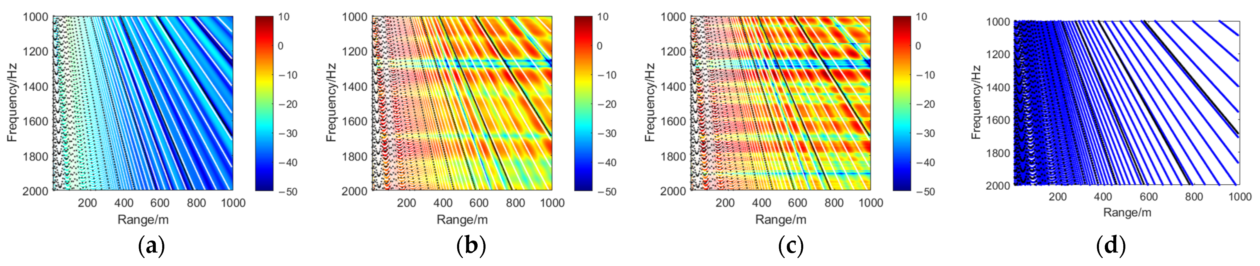
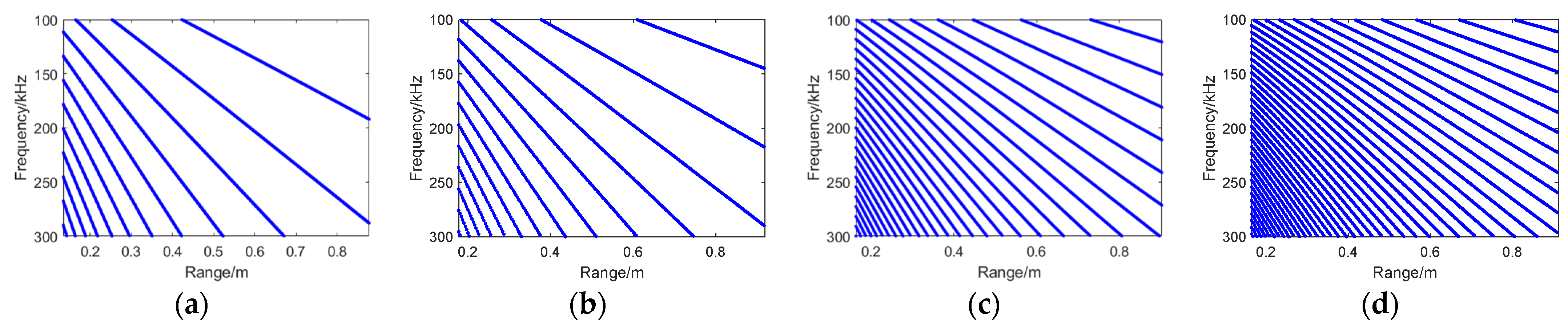
4.3. Numerical Simulation of Acoustic Fields and Interference Fringe Prediction

In Figure 6, Figure 7 and Figure 8, the black lines in subfigures (a)–(c) represent the interference patterns derived from the surface-reflected path (A1) and direct path (A0) in the model, while the white lines correspond to the interference patterns of the seafloor-reflected path (A2) and direct path (A0). However, in subfigure (d), the white lines are replaced with blue lines for clarity against the white background. Subsequent discussions focus exclusively on the black-and-white lines. The black curves in the model represent the interference patterns derived from the path differences between the sea surface-reflected path (A1) and the direct path (A0), while the white curves correspond to the interference results between the seafloor-reflected path (A2) and the direct path (A0). Notably, the number of black fringes increases with water depth, whereas the number of white fringes decreases with depth. This phenomenon is attributed to the relationship between fringe density, path differences, and wavelength.

When the path difference is small, the incremental variation in path difference relative to integer multiples of the wavelength becomes insufficient. Consequently, fewer wavelengths satisfy the constructive interference condition, resulting in sparse fringe formation over a fixed propagation distance. Conversely, larger path differences enable a greater number of wavelengths to fulfill the interference criterion, leading to densely packed fringes within the same distance.

It is observed that under identical target depths, the oblique interference fringe slopes in the channel sound field (no target), rigid sphere scattering field, and elastic sphere scattering field exhibit consistent trends. These slopes align closely with theoretical predictions derived from interference formulas, as shown in Figure 2, Figure 3 and Figure 4. This coherence underscores the pivotal role of coupling characteristics among distinct propagation paths (e.g., A0, A1, A2) within the waveguide in governing the formation of interference patterns.

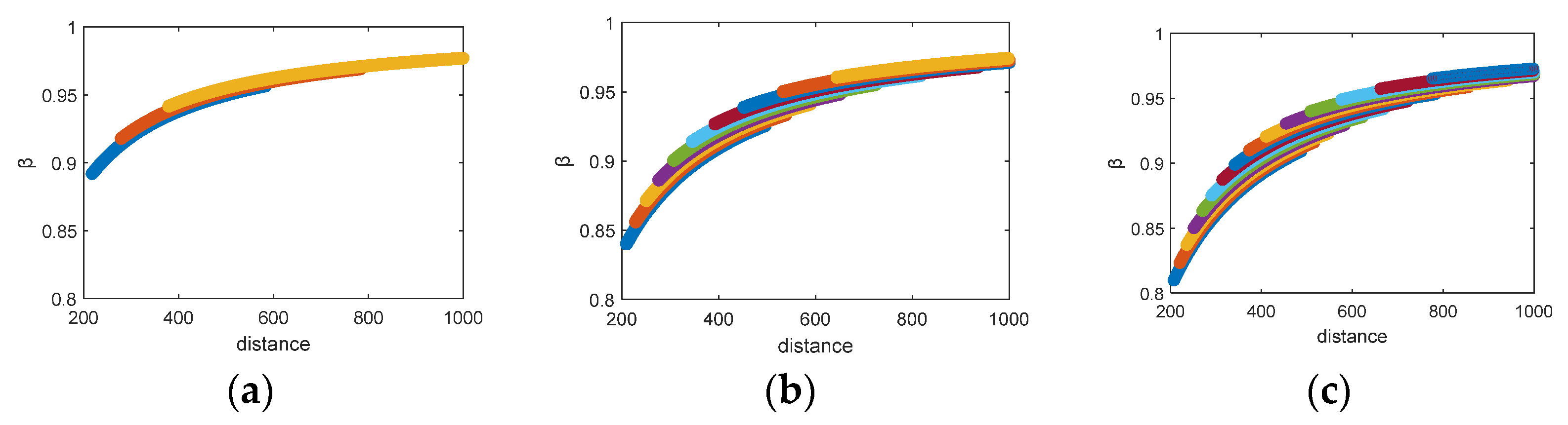
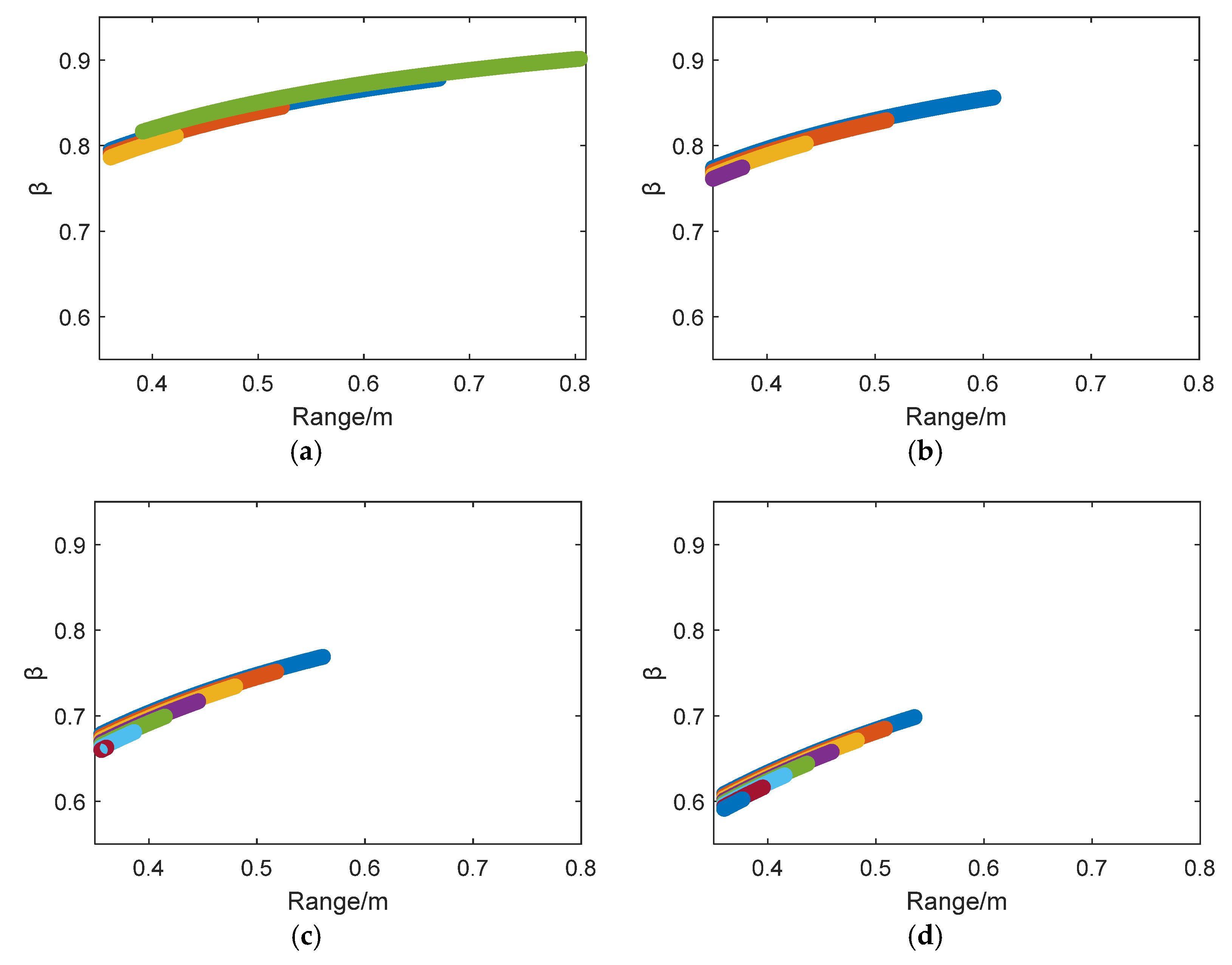
4.4. Statistical Characterization of Interference Fringes

As discussed above, the mutual interference of normal modes generates stable fringe structures in the acoustic field of a shallow-sea waveguide, manifesting as bright-dark alternating interference patterns in the range–frequency spectrum. For low-frequency broadband radiated acoustic fields, localized iso-intensity interference fringes in the sound pressure spectrogram satisfy the following expression:

$$dI(r,\omega )={\displaystyle \frac{\mathsf{\partial }I(r,\omega )}{\mathsf{\partial }r}}dr+{\displaystyle \frac{\mathsf{\partial }I(r,\omega )}{\mathsf{\partial }\omega }}d\omega =0$$

(10)

Based on the aforementioned equation, the relationship between the fringe slope in the horizontal azimuth-frequency domain and the range variation induced by relative motion between the target and receiver is governed by the following:

$${\displaystyle \frac{d\omega }{dr}}=\beta {\displaystyle \frac{\omega }{r}}$$

(11)

Equivalently,

$${\displaystyle \frac{df}{dr}}={\displaystyle \frac{f}{r}}\cdot \beta$$

(12)

By extracting the slope of fringe peaks in range–frequency spectra at varying depths and substituting these values into Equation (12), Figure 9 presents the β distributions generated by the interference between sea surface reflection paths A1 and A0 as functions of range and frequency at depths of 30 m, 50 m, and 60 m. Data points are color-coded to distinguish results from different linear fits (corresponding to the sequence of black fringes from upper right to left in Figure 6, Figure 7 and Figure 8). The results indicate that, at a given depth, the upper bound of the β approaches unity but does not represent an absolute fixed value.

Figure 10a illustrates the probability density distribution characteristics of the β across varying depths (20–65 m). It is observed that as the depth increases, the β value corresponding to the probability density peak gradually decreases. Specifically, the peak β monotonically decreases from 0.97 at 20 m to 0.93 at 65 m.

The β-peak data extracted from depths of 20–65 m are shown in Figure 10b. When constrained by 95% confidence bounds, the decreasing trend can be fitted using a linear model f(x) = p₁x + p₂f(x), yielding a root mean square error (RMSE) of 0.0009984.

5. Experimental Data Processing and Results Analysis

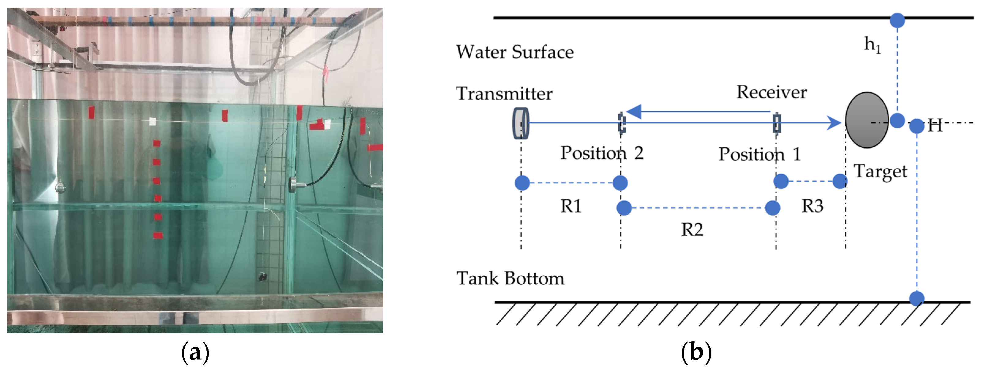
5.1. Experimental Design and Setup

To validate the accuracy of the interference frequency prediction formula for echo signals, scaled high-frequency acoustic scattering experiments were conducted in a water tank with dimensions of 2 m (length) × 1.2 m (width) × 1.6 m (height). Echo signals were collected under conditions where the hydrophone moved horizontally at a constant velocity. The acoustic source transmitted frequency-modulated (FM) signals ranging from 100 kHz to 300 kHz with a pulse width of 0.01 ms. The experimental setup was configured as follows: the water depth H was 1.5 m; the acoustic source was directed perpendicular to the target center; the source, hydrophone, and target centroid were collinear in the horizontal plane. The source and target remained stationary, while the receiving hydrophone moved from Position 1 to Position 2. The horizontal displacement of the hydrophone (R2) was 74 cm, with Position 1 located R1 = 13.5 cm from the target and Position 2 positioned (R3) 15.9 cm from the transmitting transducer. The vertical distance from the target to the water surface (h₁) and the horizontal distance from the target to the right tank wall were set to 63.5 cm. A stainless-steel sphere with a diameter of 5 cm was deployed at submerged depths of h₁ = 5 cm, 10 cm, 15 cm, and 20 cm below the water surface. During the experiment, the hydrophone moved away from the target at a constant velocity while continuously acquiring echo signals. The configuration is illustrated in Figure 11.

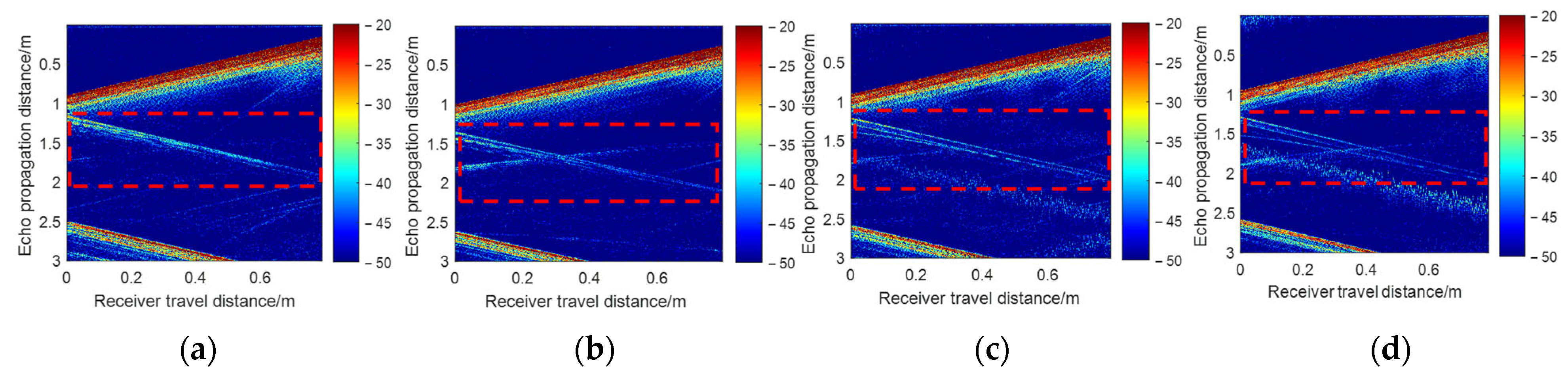
5.2. Time-Domain Echo Characteristics and Analysis

Under the specified operational and geometric conditions, time-domain echoes at varying depths are obtained by moving the hydrophone away from the target, as illustrated in Figure 12. The horizontal axis in the figure denotes the distance the hydrophone has moved. Figure 13 presents magnified views of the target echo regions under different depth conditions.

The target-scattered wave region (within the red dashed box in the figure) was truncated using a windowing method, with enlarged results of this region illustrated in Figure 12 and Figure 13. Due to the limited beam width of the transmitting transducer employed in the experiment, bottom-reflected paths were negligible when the receiver was positioned near the water surface. Three dominant acoustic wave components are clearly identified: surface-reflected waves, specularly reflected waves from the target, and elastic circumvention waves propagating around the target.

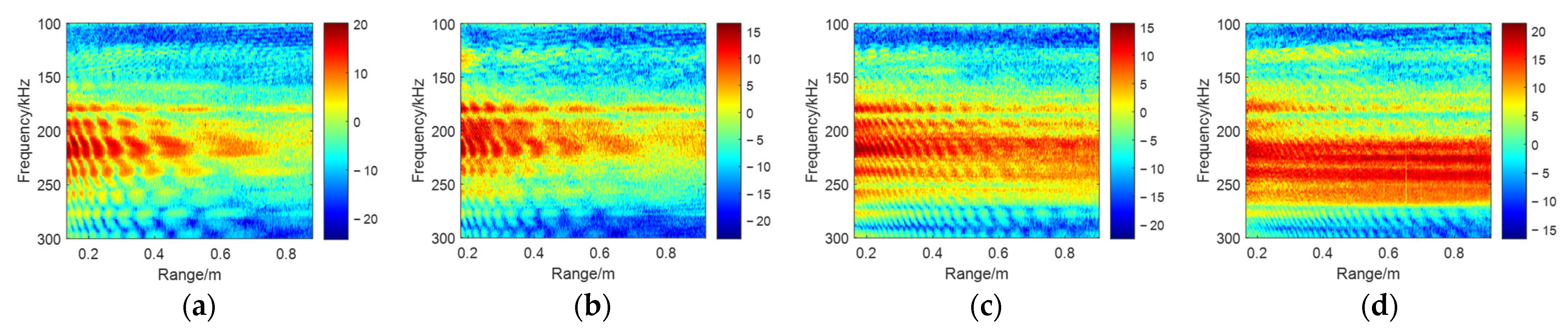
5.3. Interference Fringe Extraction and Validation

The target-scattered acoustic wave regions were extracted and subjected to Fourier transform, yielding the range–frequency spectrogram shown in Figure 14. As the source-target depth increases, the interference fringes gradually densify due to the growing path difference with depth, which increases the number of integer multiples of the wavelength satisfying the constructive interference conditions. This observation aligns with the theoretical conclusion derived from the interference formula, which establishes the relationship between path difference and wavelength. Furthermore, this phenomenon reflects the fundamental nature of wave interference, where the coupling of wavelength and path difference directly governs fringe density. Transverse resonance phenomena induced by elastic circumferential waves are distinctly visible in the frequency-range spectrum.

To validate the accuracy of the frequency interference formula, depth-dependent parameters, and motion-induced range variations were incorporated into the formula for the four tested depths. The resulting fitting curves, presented in Figure 14 and Figure 15, demonstrate high consistency between the predicted interference fringes and the experimental range–frequency spectral patterns, confirming the formula’s robustness in characterizing waveguide-coupled scattering dynamics under varying depth conditions.

6. Results and Discussion

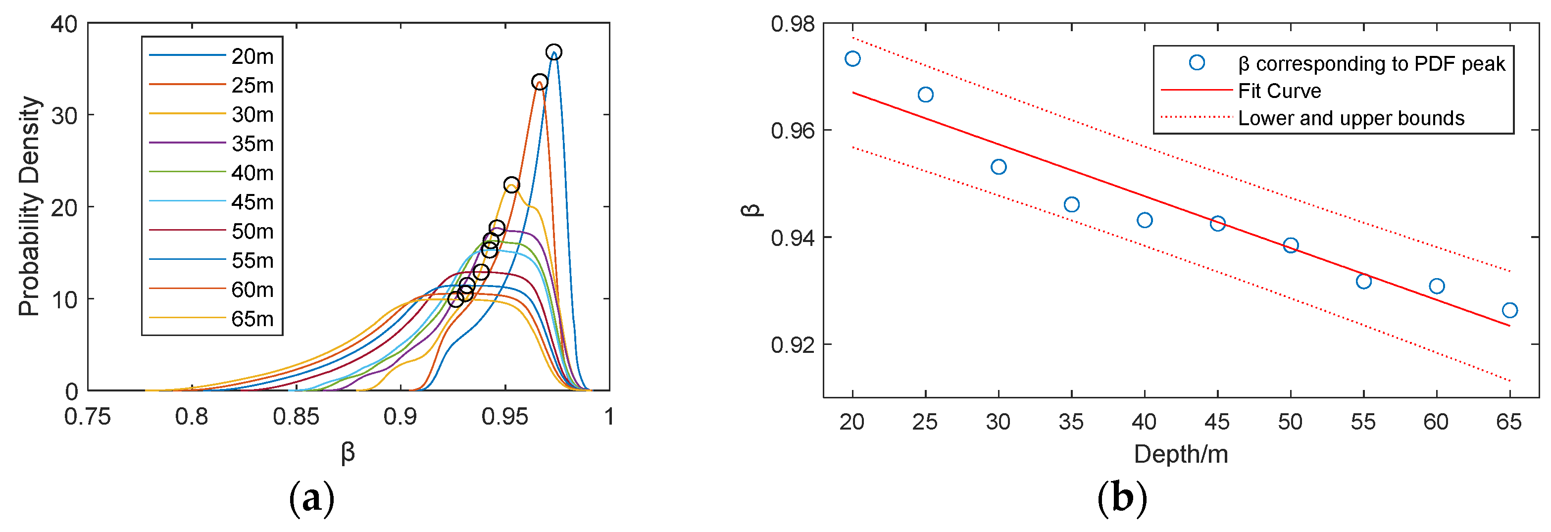
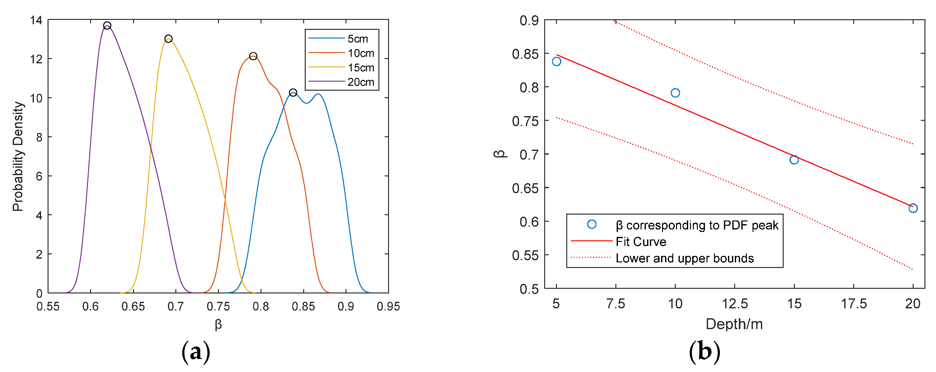
6.1. Statistical Characterization of Waveguide Invariants

By extracting the interference fringe peaks from the experimental range–frequency spectra and ignoring those peaks beyond the target range of 0.35 m along with their corresponding frequencies, the numerical ranges and probability density distributions of the β at varying depths were calculated using Equation (10). The data points, color-coded to distinguish β values derived from different linear fits (e.g., the sequence of blue fringes from the lower right to left in Figure 15), are illustrated in Figure 16.

As shown in Figure 17a, as the depth increases from 5 cm to 20 cm, the overall distribution of the β shifts downward, with the probability density peak corresponding to the β monotonically decreasing from 0.84 to 0.62. For the derived probability density peaks, a linear model f(x) = p₁x + p₂ was applied with 95% confidence bounds, consistent with the theoretical analysis (Figure 17b). The goodness-of-fit metrics confirm the model’s high accuracy. The results reveal that the β is not a fixed constant but varies with source and target depths, while its probability density gradually diminishes at shallower depths, aligning with theoretical simulations.

This trend is attributed to variations in acoustic propagation paths and dispersion characteristics: at shallower depths, stronger multipath reflections from the sea surface intensify interference effects and frequency coupling. These findings elucidate the depth-dependent evolution of acoustic interference structures in shallow-sea waveguides, providing critical insights for optimizing algorithms in source depth estimation and waveguide parameter inversion.

6.2. Comparative Analysis

This study constructs a coupled normal mode and scattering function model, addressing the limitations of conventional approaches that independently apply normal mode or ray theory without integrating target scattering effects. The model elucidates the coupling mechanism between multipath acoustic interference and target scattering, demonstrating how the interference superposition of acoustic waves from distinct paths at the receiver modulates the spatial distribution and frequency-dependent characteristics of the scattered field.

To overcome the shortcomings of prior research on the β, which predominantly relied on qualitative analysis of single environmental parameters or numerical simulations under fixed frequency and depth conditions. This work employs theoretical simulations and scaled experiments to quantitatively reveal the relationship between β-value ranges and water depth.

A summary of the theoretical waveguide invariant (β) ranges and their corresponding probability density peaks are presented in

Table 3. Numerical ranges of the β from theoretical simulations.

Depth/m	Waveguide Invariant Range/β	Probability Density Peak/β
20	0.91–0.98	0.97
30	0.89–0.98	0.95
40	0.86–0.98	0.94
50	0.84–0.98	0.93
60	0.81–0.98	0.92

, which displays the numerical ranges of β, frequency bands, and probability density peaks at water depths of 20 m, 30 m, 40 m, 50 m, and 60 m. The results demonstrate that as water depth increases, the β-values gradually decrease: at 20 m depth, the range spans 0.91–0.98, decreasing to 0.86–0.98 at 40 m, and further contracting to 0.81–0.98 at 60 m. Concurrently, the variability of β-values expands with increasing depth, indicating greater dispersion in waveguide invariant statistics under deeper conditions. Additionally, the probability density peaks exhibit a systematic decline, decreasing from 0.97 at 20 m to 0.94 at 40 m and 0.92 at 60 m.

The experiment β ranges and corresponding probability density peaks, summarized in

Table 4. The comparison of peak extraction and prediction formula for β.

Depth/cm	Waveguide Invariant Range/β		Probability Density Peak/β
	Prediction Formula	Peak Extraction	Prediction Formula	Peak Extraction
5	0.76–0.90	0.66–0.91	0.83	0.79
10	0.75–0.85	0.70–0.87	0.79	0.77
15	0.66–0.76	0.61–0.72	0.69	0.67
20	0.59–0.69	0.60–0.70	0.61	0.63

, were determined using both peak extraction calculations and prediction formula calculations. The experiments demonstrate that as water depth increases from 5 cm to 20 cm: the β-value range narrows progressively across both calculation methods; simultaneously, the probability density peaks exhibit a systematic reduction.

7. Results and Conclusions

In summary, this study investigates the formation mechanisms of interference fringes during acoustic wave propagation and their relationship with the waveguide invariant (β). Through integrated theoretical analysis and experimental validation, the influence of multipath effects on interference fringes in range–frequency spectra is elucidated. By employing a fringe-fitting analytical method to calculate interference peak trajectories and slopes, precise extraction of the β is achieved, and its variation patterns are thoroughly explored. The results demonstrate that the β is not a fixed value but fluctuates within a specific range depending on frequency and depth. Theoretical simulations reveal that as water depth increases, the numerical range of the β progressively narrows, accompanied by a decline in probability density peak magnitudes—a trend corroborated by experimental data. The theoretical framework, based on shallow water environments (20 m to 65 m) and low-frequency bands (1–2 kHz), delineates the macro-scale evolution of β. Experimental studies conducted using scaled models and high-frequency sources (100–300 kHz) further validate these statistical characteristics through prediction formula calculations and peak extraction methods. By quantifying β ranges and probability density peaks across depths, this work establishes a robust methodology for analyzing acoustic wave propagation in channelized environments, providing critical insights into target localization and scattering field dynamics under complex waveguide conditions.

References

1. Zhang, P.; Zhou, G.; Fan, J.; Wang, B.; Feng, Z. Analysis of acoustic scattering mechanism of a near-bottom suspended elastic sphere. Acta Acust. 2024, 49, 880–888. [Google Scholar] [CrossRef]
2. Sun, T.; Yan, Z.; Fan, J.; Zhang, H. Method for Characterizing Active Sonar Interference Fringes Based on the Sum of Curvature. Comput. Eng. 2022, 48, 49–54. [Google Scholar] [CrossRef]
3. Dzenis, N.L.; Chuprov, S.D. Influence of Motion of a Monochromatic Source on the Spatial Interference Structure of the Field in a Plane-layered Waveguide. Sov. Phys. Acoust. 1986, 32, 242–243. [Google Scholar]
4. Su, X.; Zhang, R.; Li, F. Calculation of the waveguide invariant of acoustic fields by using frequency-shift compensation method. Tech. Acoust. 2007, 26, 1073–1076. [Google Scholar] [CrossRef]
5. He, C.; Quijano, J.E.; Zurk, L.M. Enhanced Kalman filter algorithm using the invariance principle. IEEE J. Ocean. Eng. 2009, 34, 575–585. [Google Scholar]
6. Zhu, H.; Piao, S.; Zhang, H.; Liu, W. An extraction method for the interference striation of acoustic vector fields in shallow water. Acta Acust. 2016, 41, 30–40. [Google Scholar]
7. Lu, L.; Ma, L. Analysis of waveguide time-frequency based on Warping transform. Acta Phys. Sin. 2015, 64, 297–302. [Google Scholar]
8. Yao, Y.; Sun, C.; Liu, X.H.; Li, M. Waveguide invariant estimation based on correlation coefficient of tonal acoustic intensity interference fluctuation. J. Northwestern Polytech. Univ. 2023, 41, 612–620. [Google Scholar] [CrossRef]
9. Mo, S.; Wang, B.; Li, T. Vector waveguide invariant estimation based on the lines segment detector algorithm. J. Harbin Eng. Univ. 2023, 44, 1748–1757. [Google Scholar]
10. Li, M.; Zhao, A.; Song, X. Waveguide invariant extraction technique in shallow water. In Proceedings of the 2017 National Conference on Acoustics, Hangzhou, China, 22 September 2017. [Google Scholar]
11. Li, M. Extraction Techniques for Waveguide Invariants in Shallow-Sea Acoustic Fields. Ph.D. Thesis, Harbin Engineering University, Harbin, China, 2017. [Google Scholar]
12. Liu, Z.; Guo, L.; Yan, C. Source depth discrimination in negative thermocline using waveguide invariant. Acta Acust. 2019, 44, 925–933. [Google Scholar]
13. Wang, W.; Su, L.; Wang, Z.; Hu, T.; Ren, Q.; Guo, S.; Ma, L. A broadband source depth estimation based on frequency domain interference pattern structure of vertical array beam output in direct zone of deep sea. Acta Acust. 2021, 46, 161–170. [Google Scholar]
14. Dun, J.; Zhou, S.; Qi, Y.; Liu, C. Simulation Study on Detection and Localization of a Moving Target Under Reverberation in Deep Water. J. Mar. Sci. Eng. 2024, 12, 2360. [Google Scholar] [CrossRef]
15. Xu, J.; Guo, L.; Yan, C. Source depth estimation using frequency domain interference structure in deep ocean bottom bounce area. Acta Acust. 2023, 48, 425–436. [Google Scholar]
16. Li, X.; Wang, B.; Bi, X.; Wu, H. A fast inversion method for ocean parameters based on dispersion curves with a single hydrophone. Acta Oceanol. Sin. 2022, 41, 71–85. [Google Scholar] [CrossRef]
17. Zhai, Z.; Li, F.; Zhang, B.; Zhai, Z.; Hu, C. Broadband source localization by matching interference structure in the direct zone of deep water using a bottom-mounted horizontal array. Acta Acust. 2025, 5, 433–444. [Google Scholar] [CrossRef]
18. Zakharenko, A.; Trofimov, M.; Petrov, P. Improving the performance of mode-based sound propagation models by using perturbation formulae for eigenvalues and eigenfunctions. J. Mar. Sci. Eng. 2021, 9, 934. [Google Scholar] [CrossRef]
19. Kozitskiy, S. Coupled-mode parabolic equations for the modeling of sound propagation in a shallow-water waveguide with weak elastic bottom. J. Mar. Sci. Eng. 2022, 10, 1355. [Google Scholar] [CrossRef]
20. Su, X.; Qin, J.; Yu, X. Interference Pattern Anomaly of an Acoustic Field Induced by Bottom Elasticity in Shallow Water. J. Mar. Sci. Eng. 2023, 11, 647. [Google Scholar] [CrossRef]
21. Mei, X.; Zhang, B.; Zhai, D. Bearing-Only Multi-Target Localization Incorporating Waveguide Characteristics for Low Detection Rate Scenarios in Shallow Water. J. Mar. Sci. Eng. 2024, 12, 2300. [Google Scholar] [CrossRef]
22. Ingenito, F. Scattering from an object in a stratified medium. J. Acoust. Soc. Am. 1987, 82, 2051–2059. [Google Scholar] [CrossRef]
23. Folds, D.L.; Loggins, C.D. Transmission and reflection of ultrasonic waves in layered media. J. Acoust. Soc. Am. 1977, 62, 1102–1109. [Google Scholar] [CrossRef]
24. Quijano, J.E.; Campbell, R.L.; Oesterlein, T.G. Experimental observations of active invariance striations in a tank environment. J. Acoust. Soc. Am. 2010, 128, 611–618. [Google Scholar] [CrossRef] [PubMed]
25. Lan, C.; Zhang, H. Calculation and measurement of the propagation velocity of the Franz wave. Acta Acust. 1988, 13, 147–149. [Google Scholar] [CrossRef]
26. Flax, L.; Varadan, V.K.; Varadan, V.V. Scattering of an obliquely incident acoustic wave by an infinite cylinder. J. Acoust. Soc. Am. 1980, 68, 1832–1835. [Google Scholar] [CrossRef]
27. Wu, Y. Acoustic Scattering Characteristics and Feature Extraction of Underwater Spherical and Cylindrical Objects. Ph.D. Thesis, Harbin Engineering University, Harbin, China, 2019. [Google Scholar]
Figure 1. Schematic diagram of target geometry in an ideal acoustic waveguide.
Jmse 13 01100 g001
Figure 2. Range–frequency spectrogram for source and receiver depths at 30 m. (a) Channel sound field (no target). (b) Waveguide-coupled scattered field from the rigid target. (c) Waveguide-coupled scattered field from the elastic target.
Jmse 13 01100 g002
Figure 3. Range–frequency spectrogram for source and receiver depths at 50 m. (a) Channel sound field (no target). (b) Waveguide-coupled scattered field from the rigid target. (c) Waveguide-coupled scattered field from the elastic target.
Jmse 13 01100 g003
Figure 4. Range–frequency spectrogram for source and receiver depths at 60 m. (a) Channel sound field (no target). (b) Waveguide-coupled scattered field from the rigid target. (c) Waveguide-coupled scattered field from the elastic target.
Jmse 13 01100 g004
Figure 5. Echo schematics. (a) Wave paths without target; (b) Wave paths with interface–target coupling.
Jmse 13 01100 g005
Figure 6. Interference fringes in the range–frequency spectrogram at 30 m depth. (a) Channel sound field (no target). (b) Waveguide-coupled scattered field from the rigid target. (c) Waveguide-coupled scattered field from the elastic target. (d) Pure interference fringes.
Jmse 13 01100 g006
Figure 7. Interference fringes in the range–frequency spectrogram at 50 m depth. (a) Channel sound field (no target). (b) Waveguide-coupled scattered field from the rigid target. (c) Waveguide-coupled scattered field from the elastic target. (d) Pure interference fringes.
Jmse 13 01100 g007
Figure 8. Interference fringes in the range–frequency spectrogram at 60 m depth. (a) Channel sound field (no target). (b) Waveguide-coupled scattered field from rigid the target. (c) Waveguide-coupled scattered field from the elastic target. (d) Pure interference fringes.
Jmse 13 01100 g008
Figure 9. Distance vs. β. (a) 30 m; (b) 50 m; (c) 60 m.
Jmse 13 01100 g009
Figure 10. Probability density characteristics of the β. (a) Probability density distribution of β at different depths. (b) β corresponding to the peaks of probability density at different depths.
Jmse 13 01100 g010
Figure 11. Experimental setup. (a) Photograph of the water tank. (b) Schematic diagram of target geometry in the water tank.
Jmse 13 01100 g011
Figure 12. Range–time domain echoes. (a) 5 cm; (b) 10 cm; (c) 15 cm; (d) 20 cm.
Jmse 13 01100 g012
Figure 13. Range–time domain echoes (enlarged graph). (a) 5 cm; (b) 10 cm; (c) 15 cm; (d) 20 cm.
Jmse 13 01100 g013
Figure 14. Range–frequency spectrum at different depths. (a) 5 cm; (b) 10 cm; (c) 15 cm; (d) 20 cm.
Jmse 13 01100 g014
Figure 15. Pure interference fringe at different depths. (a) 5 cm; (b) 10 cm; (c) 15 cm; (d) 20 cm.
Jmse 13 01100 g015
Figure 16. Distance vs. β. (a) 5 cm; (b) 10 cm; (c) 15 cm; (d) 20 cm.
Jmse 13 01100 g016
Figure 17. Probability density characteristics of the β. (a) Probability density distributions of the β at varying depths. (b) β values corresponding to probability density peaks across depths.
Jmse 13 01100 g017