Development and Performance Analysis of a Novel Wave Energy Converter Based on Roll Movement: A Case Study in the BiMEP

 and
and
Abstract
1. Introduction
2. Material and Methods
2.1. Device Description and Situation
2.2. Analysis of Wave Characteristics
- ≥1%, green, representing 27.96% of all the waves of these types.
- 0.75% to 0.999%, blue, representing 20.47% of all the waves of these types.
- 0.5% to 0.749%, yellow, representing 18.17% of all the waves of these types.
- 0.25% to 0.499%, orange, representing 22.07% of all the waves of these types.
- <0.25%, red, representing 11.34% of all the waves of these types.
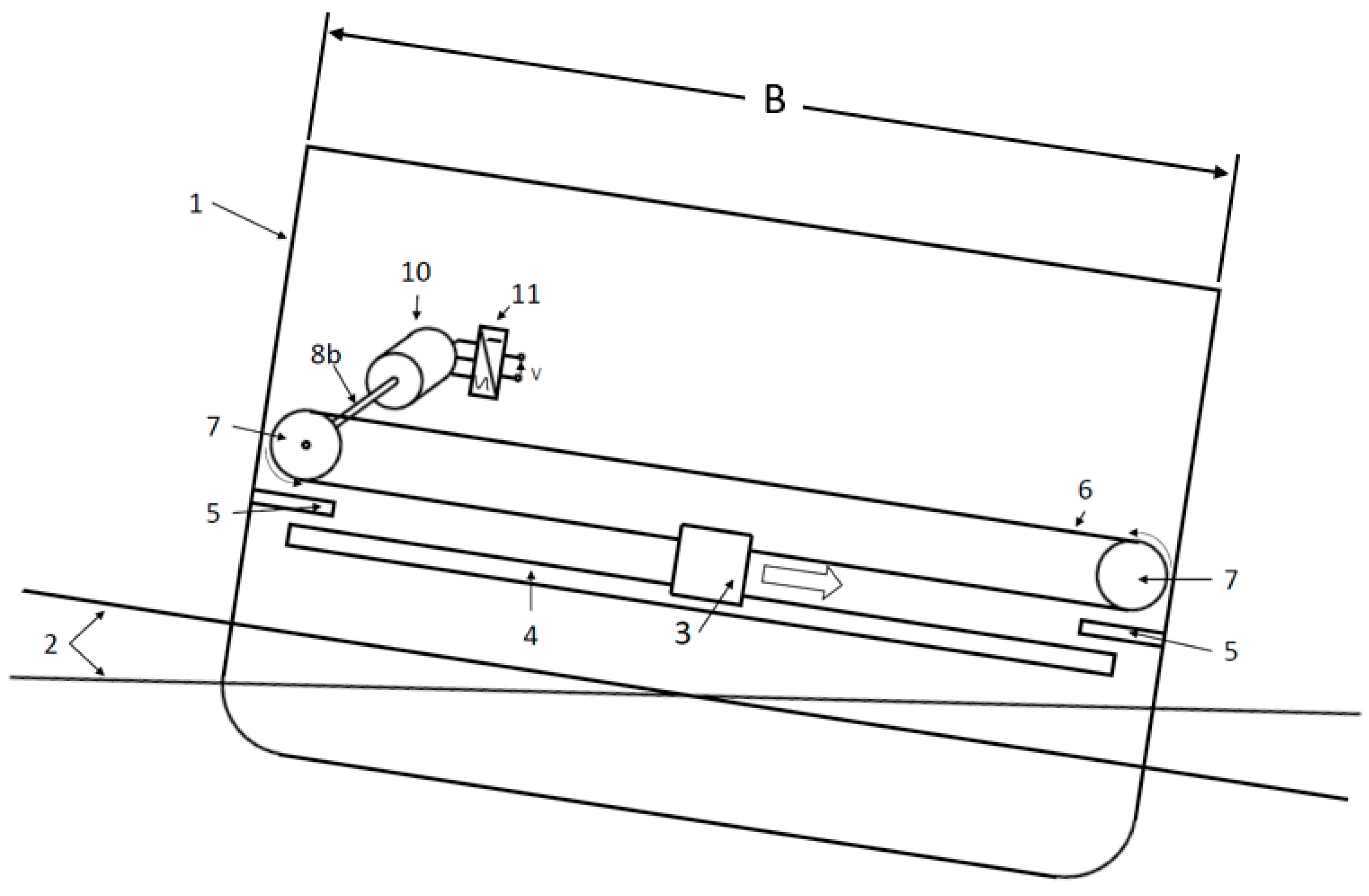
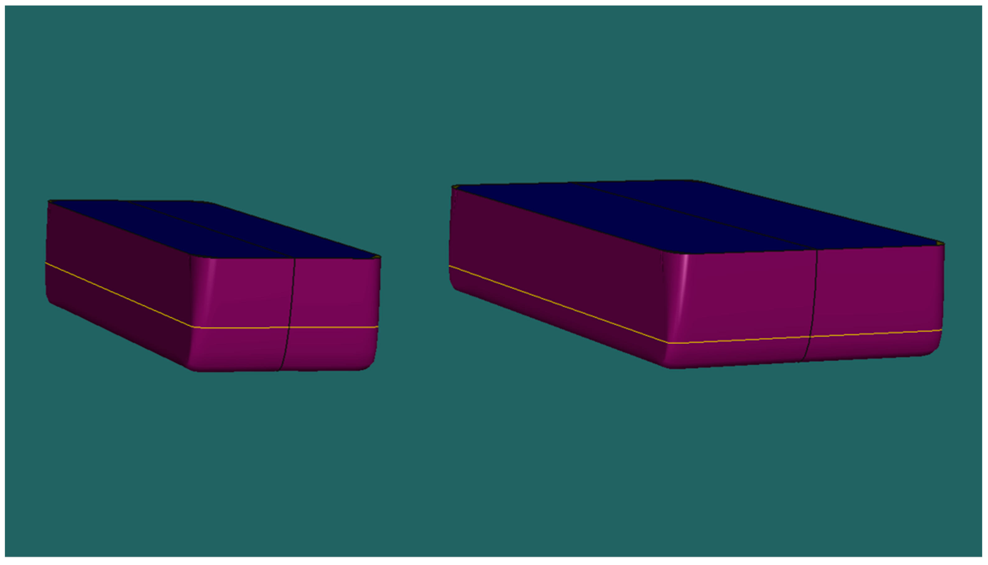
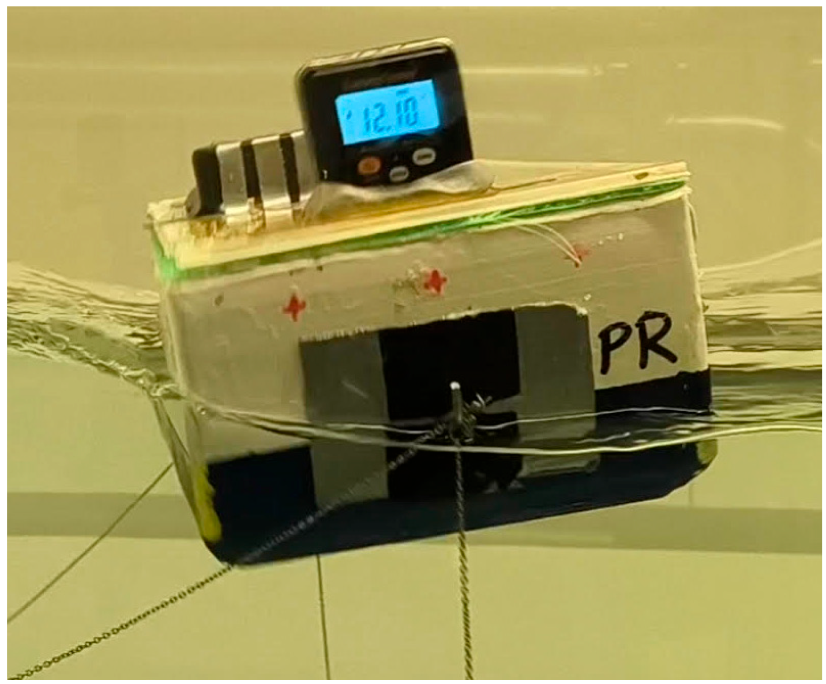
2.3. Model Design
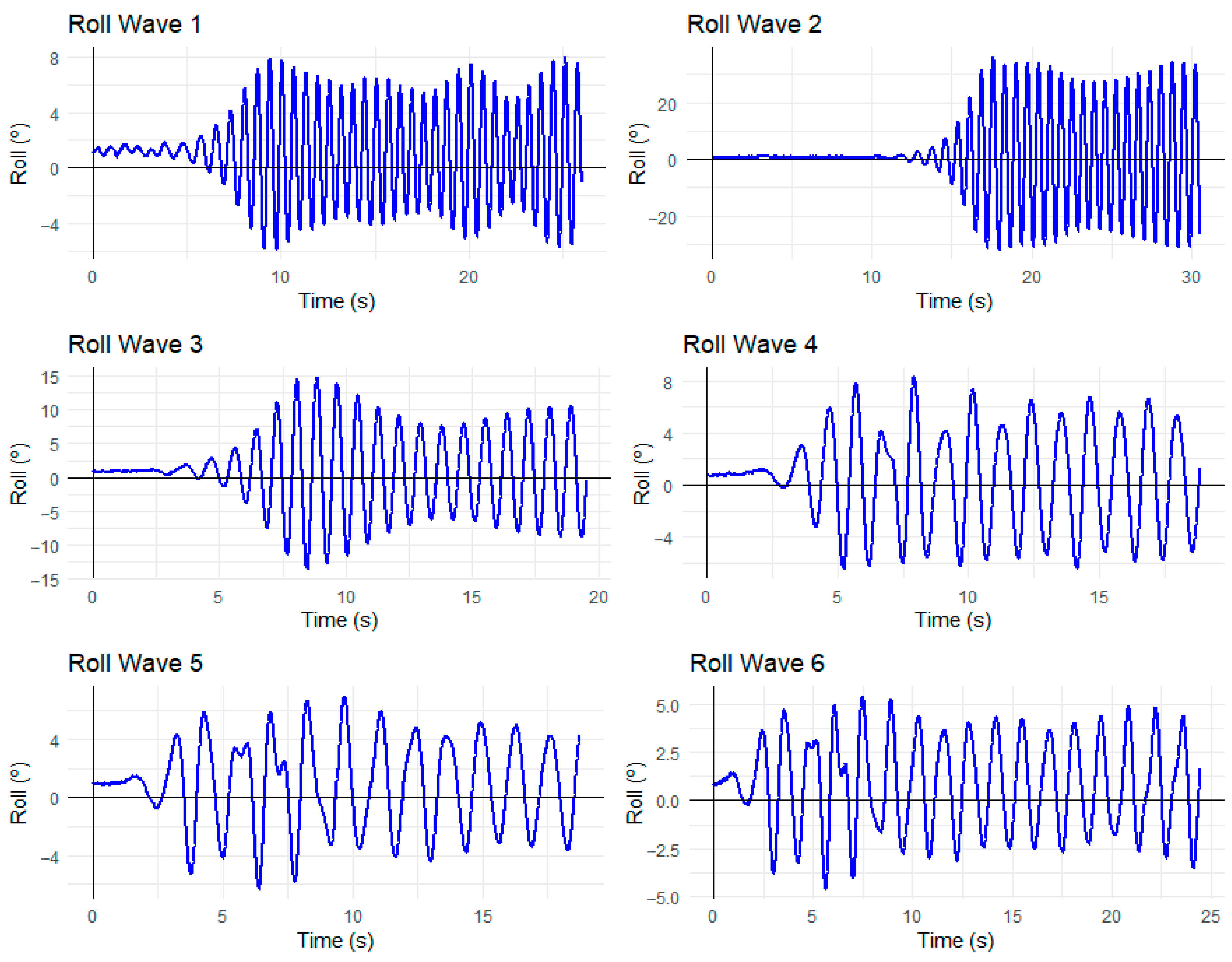
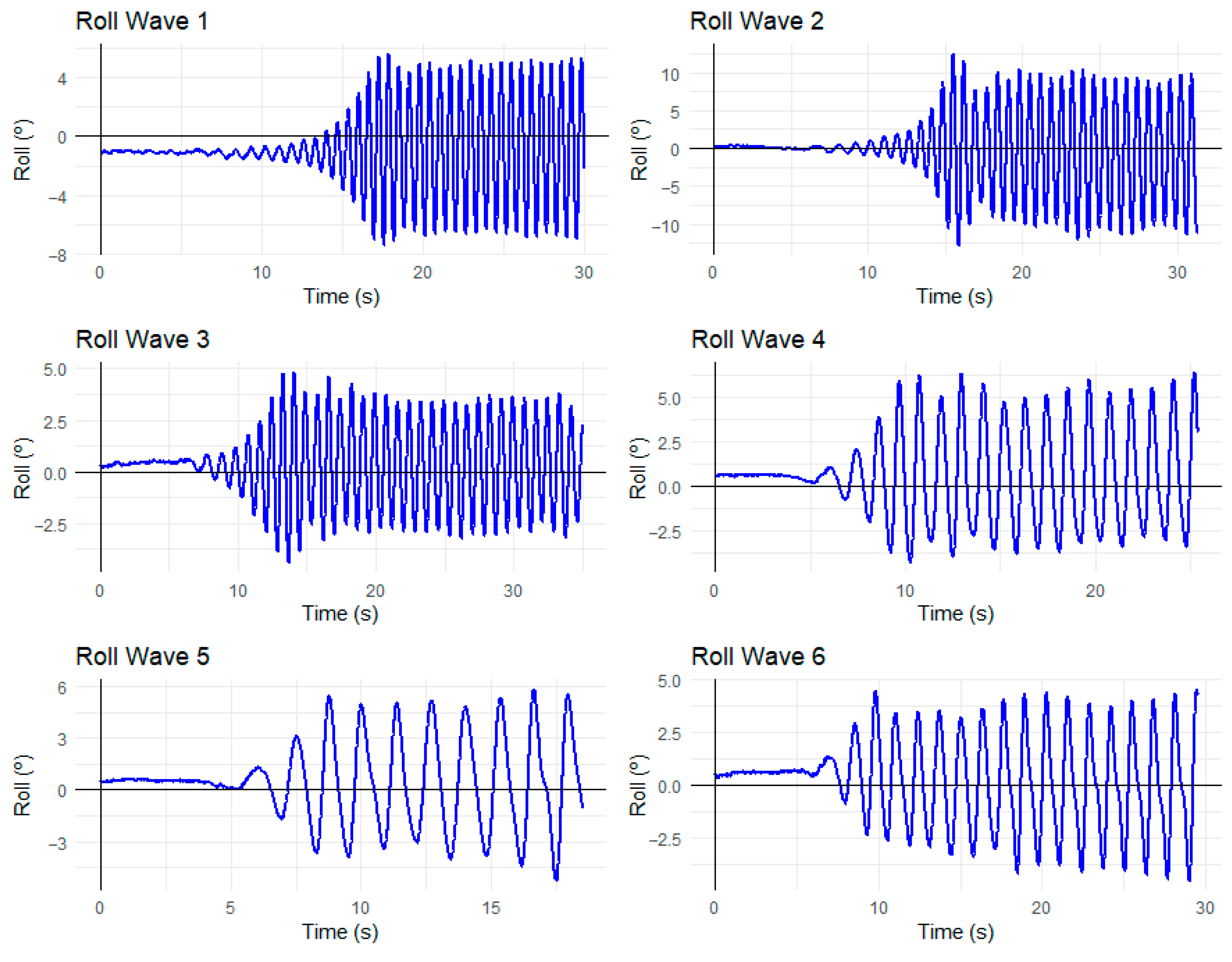
2.4. Wave Tank Tests
- (1)
- 4.50 s and 1.00 m;
- (2)
- 5.00 s and 2.25 m;
- (3)
- 6.00 s and 1.25 m;
- (4)
- 8.00 s and 2.00 m;
- (5)
- 9.50 s and 2.25 m;
- (6)
- 9.50 s and 1.75 m.
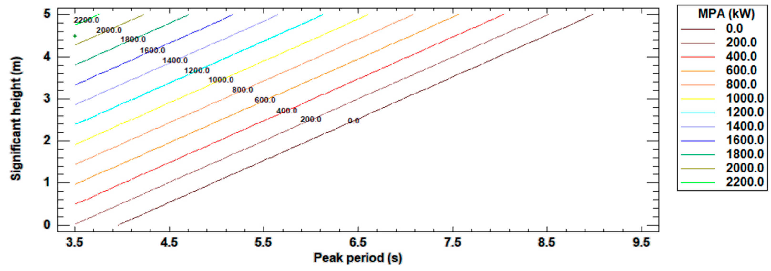
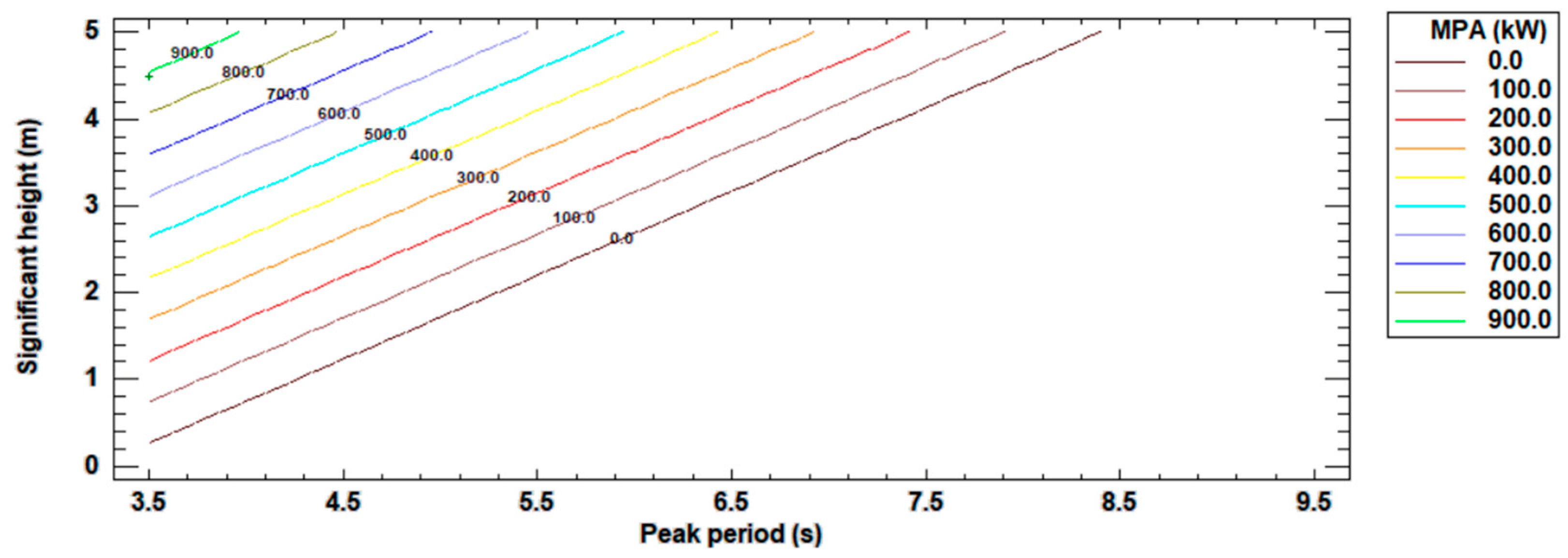
2.5. Maximum Theorical Power Calculation
- (1)
- 3.5 s and 0.5 m;
- (2)
- 9.5 s and 0.5 m;
- (3)
- 3.5 s and 5 m;
- (4)
- 9.5 s and 5 m.
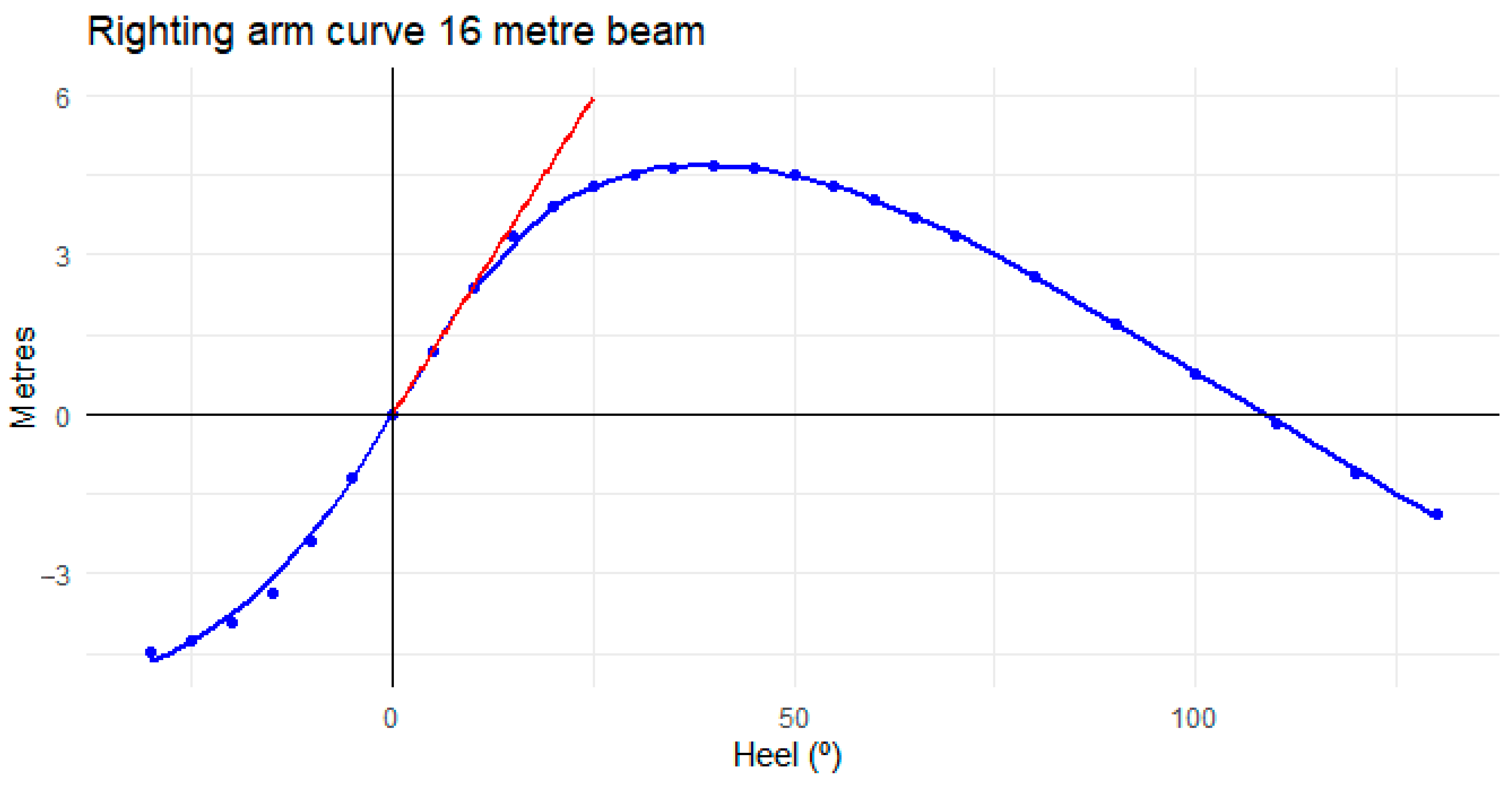
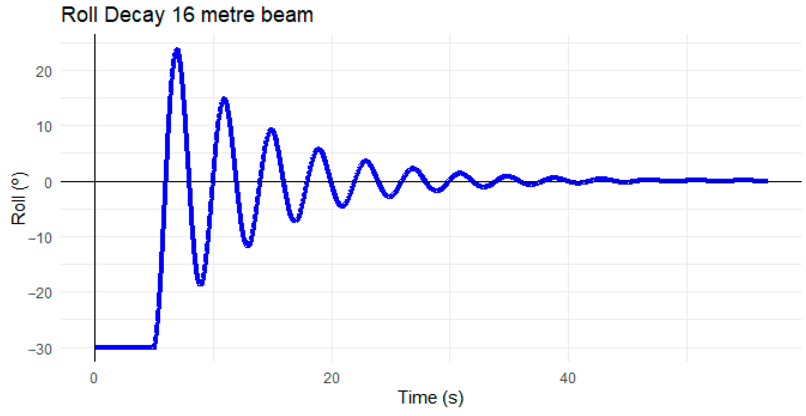
3. Results
4. Conclusions
Author Contributions
Funding
Data Availability Statement
Conflicts of Interest
References
- United Nations. Framework Convention on Climate Change. In Adoption of the Paris Agreement; United Nations: New York, NY, USA, 2015. [Google Scholar]
- European Commision. A Clean planet for all. In A European Strategic Long-Term Vision for a Prosperous, Modern, Competitive and Climate Neutral Economy; European Commission: Brussels, Belgium, 2018. [Google Scholar]
- European Commission. National Energy and Climate Plans (NECPs); European Commission: Brussels, Belgium, 2020. [Google Scholar]
- García, X.; Domínguez, J.; Linares, P.; López, O. Renovables 2050. In Un Informe Sobre el Potencial de las Energías Renovables en la España peninsular; Informe del Instituto de Investigaciones Tecnológicas de la Universidad Pontificia de Comillas para Greenpeace: Comillas, Spain, 2005. [Google Scholar]
- Llinás, O. La plataforma Oceánica de Canarias (PLOCAN): Infraestructura de Referencia para la Investigación, Desarrollo Tecnológico e Innovación Marino-Marítima; Universidad de Málaga: Málaga, Spain, 2019. [Google Scholar]
- Del Río-Gamero, B.; Alecio, T.L.; Schallenberg-Rodríguez, J. Performance indicators for coupling desalination plants with wave energy. Desalination 2022, 525, 115479. [Google Scholar] [CrossRef]
- Zhou, Z.; Ke, S.; Wang, R.; Mayon, R.; Ning, D. Hydrodynamic investigation on a land-fixed OWC wave energy device under irregular waves. Appl. Sci. 2022, 12, 2855. [Google Scholar] [CrossRef]
- Stratigaki, V.; Mouffe, L. Ocean energy in belgium-2019. OES Annu. Rep. 2019, 2019, 48–53. [Google Scholar]
- Cabeza Pindado, Á. Evaluación de la Accesibilidad Buque-Plataforma en el Parque de Pruebas BIMEP (País Vasco) Ante las Condiciones Climáticas Marinas; Universidad de Cantabria: Santander, Spain, 2016. [Google Scholar]
- Weller, S.D.; Parish, D.; Gordelier, T.; de Miguel Para, B.; Garcia, E.A.; Goodwin, P.; Tornroos, D.; Johanning, L. Open Sea OWC Motions and Mooring Loads Monitoring at BiMEP; University of Exeter: Exeter, UK, 2017. [Google Scholar]
- Uriarte, A.; Boyra, G.; Ferarios, J.M.; Gabiña, G.; Lasa, J.; Quincoces, I.; Beatriz, S.; Bald, J. ITSASDRONE, an autonomous marine surface drone for fish monitoring around wave energy devices. In Proceedings of the European Wave and Tidal Energy Conference, Bilbao, Spain, 3–7 September 2023. [Google Scholar]
- Park, J.; Baek, H.; Shim, H.; Choi, J. Preliminary investigation for feasibility of wave energy converters and the surrounding sea as test-site for marine equipment. J. Ocean Eng. Technol. 2020, 34, 351–360. [Google Scholar] [CrossRef]
- Qin, S.; Fan, J.; Zhang, H.; Su, J.; Wang, Y. Flume experiments on energy conversion behavior for oscillating buoy devices interacting with different wave types. J. Mar. Sci. Eng. 2021, 9, 852. [Google Scholar] [CrossRef]
- Gomes, R.; Henriques, J.; Gato, L.; Falcao, A. Testing of a small-scale floating OWC model in a wave flume. In Proceedings of the International Conference on Ocean Energy, Dublin, Ireland, 17–19 October 2012; 1p. [Google Scholar]
- Bacelli, G.; Haegmueller, A.; Ginsburg, M.; Gunawan, B. Characterizing the Dynamic Behavior and Performance of a Scaled Prototype Point Absorber Wave Energy Converter in a Large Wave Flume. In Proceedings of the 13th European Wave and Tidal Energy Conference, Naples, Italy, 1–6 September 2019. [Google Scholar]
- Sugiura, K.; Sawada, R.; Nemoto, Y.; Haraguchi, R.; Asai, T. Wave flume testing of an oscillating-body wave energy converter with a tuned inerter. Appl. Ocean Res. 2020, 98, 102127. [Google Scholar] [CrossRef]
- Wang, D.; Qiu, S.; Ye, J. An experimental study on a trapezoidal pendulum wave energy converter in regular waves. China Ocean Eng. 2015, 29, 623–632. [Google Scholar] [CrossRef]
- Minguela, J.P.R.; Fadrique, S.E.; Eizmendi, M.H.; Loza, P.L. Installation and Method for Harnessing Wave Energy. U.S. Patent No 7,906,865, 15 March 2011. [Google Scholar]
- Salcedo, F.; Ruiz-Minguela, P.; Rodriguez, R.; Ricci, P.; Santos, M. Oceantec: Sea trials of a quarter scale prototype. In Proceedings of the 8th European Wave Tidal Energy Conference, Uppsala, Sweden, 7–10 September 2009; 460p. [Google Scholar]
- Bauer, P.; Dillon-Gibbons, C.; Iyer, N.; Kilner, A.; Easson, A.; Gumley, J.; Thurumella, H. Numerical analysis of a wave energy converter. In Proceedings of the Offshore Technology Conference OTC, Houston, TX, USA, 1–4 May 2023. [Google Scholar]
- Cordonnier, J.; Gorintin, F.; De Cagny, A.; Clément, A.H.; Babarit, A. SEAREV: Case study of the development of a wave energy converter. Renew. Energy 2015, 80, 40–52. [Google Scholar] [CrossRef]
- Ruellan, M.; BenAhmed, H.; Multon, B.; Josset, C.; Babarit, A.; Clement, A. Design methodology for a SEAREV wave energy converter. IEEE Trans. Energy Convers. 2010, 25, 760–767. [Google Scholar] [CrossRef]
- Pozzi, N. Numerical Modeling and Experimental Testing of a Pendulum Wave Energy Converter (PeWEC); Politecnico Di Torino: Torino, Italy, 2018. [Google Scholar]
- Pozzi, N.; Bracco, G.; Passione, B.; Sirigu, S.A.; Mattiazzo, G. PeWEC: Experimental validation of wave to PTO numerical model. Ocean Eng. 2018, 167, 114–129. [Google Scholar] [CrossRef]
- Turkia, J. Potential of Wave Power: A Techno-Economic Feasibility Analysis of Gyration Based Wave Energy Technology; Tampere University: Tampere, Finland, 2015. [Google Scholar]
- Drew, B.; Plummer, A.R.; Sahinkaya, M.N. A Review of Wave Energy Converter Technology. Proc. Inst. Mech. Eng. Part A J. Power Energy 2009, 223, 887–902. [Google Scholar] [CrossRef]
- Solaeche, M.A.G.; Barrena, J.L.L.; Falces, D.B.; Diego, I.B.; Arraiza, A.L.; Lavín, E.U.; Cabezudo, J.B. Wave Energy to Electrical Energy Converter. WO2024/209063A1, 10 October 2024. Available online: https://patentimages.storage.googleapis.com/2a/f6/f7/a92fceb772230f/WO2024209063A1.pdf (accessed on 12 February 2025).
- Olivella Puig, J. Teoría del Buque. Ola Trocoidal, Movimientos y Esfuerzo; Universitat Politècnica de Catalunya, Iniciativa Digital Politècnica: Barcelona, Spain, 1998. [Google Scholar]
- Guo, B.; Ringwood, J.V. A review of wave energy technology from a research and commercial perspective. IET Renew. Power Gener. 2021, 15, 3065–3090. [Google Scholar] [CrossRef]
- Metocean Analysis of BiMEP for Offshore Design [Internet]. 2017. Available online: http://www.trlplus.es/ (accessed on 12 March 2020).
- Velasco González, F.J.; Vega, L.M.; Revestido, E.; Javier, F.; Santos, L.; Terán Fernández, J. Laboratorio marino remoto aplicado a la experimentación en tecnología naval. In Proceedings of the Actas de las XXXVI Jornadas de Automática, Bilbao, Spain, 2–4 September 2015. [Google Scholar]
- Bhattacharyya, R. Dynamics of Marine Vehicles; John Wiley & Sons Incorporated: Hoboken, NJ, USA, 1978. [Google Scholar]
- Quality Systems Group of the 28th ITTC. ITTC-Recommended Procedures and Guidelines Numerical Estimation of Roll Damping. Zurich, Switzerland. 2011. Available online: https://ittc.info/media/1343/75-02-07-045.pdf (accessed on 14 April 2025).
- Ogata, K. Ingeniería de Control Moderna; Pearson Educación: London, UK, 2003. [Google Scholar]
- Kianejad, S.S.; Enshaei, H.; Duffy, J.; Ansarifard, N. Prediction of a ship roll added mass moment of inertia using numerical simulation. Ocean Eng. 2019, 173, 77–89. [Google Scholar] [CrossRef]
- Mezcua, J.; Gil, A.; Benarroch, R. Estudio Gravimétrico de la Península Ibérica y Baleares; Instituto Geográfico Nacional: Madrid, Spain, 1996. [Google Scholar]


| Peak Period(s) | ||||||||||||||||||||||||
|---|---|---|---|---|---|---|---|---|---|---|---|---|---|---|---|---|---|---|---|---|---|---|---|---|
| 2 | 2.5 | 3 | 3.5 | 4 | 4.5 | 5 | 5.5 | 6 | 6.5 | 7 | 7.5 | 8 | 8.5 | 9 | 9.5 | 10 | 10.5 | 11 | 11.5 | 12 | 12.5 | Total | ||
| Significant wave height (m) | 0.5 | 0.11 | 0.29 | 1.09 | 1.09 | 0.17 | 0.20 | 0.17 | 0.11 | 0.03 | 0.03 | 0.06 | - | - | - | - | - | - | - | - | - | - | - | 3.36 |
| 0.75 | 0.06 | 0.80 | 0.92 | 1.75 | 0.95 | 0.83 | 0.32 | 0.63 | 0.32 | 0.23 | 0.03 | - | - | - | - | - | - | - | - | - | - | - | 6.83 | |
| 1 | - | 0.06 | 0.63 | 2.30 | 0.89 | 1.38 | 0.89 | 0.86 | 0.92 | 0.92 | 0.43 | 0.17 | 0.26 | 0.29 | 0.14 | 0.03 | - | - | - | - | - | - | 10.16 | |
| 1.25 | - | 0.03 | 0.52 | 0.49 | 0.34 | 0.49 | 0.77 | 1.21 | 1.44 | 1.32 | 0.46 | 0.63 | 0.52 | 0.55 | 0.11 | 0.03 | - | 0.06 | - | - | - | - | 8.96 | |
| 1.5 | - | - | 0.17 | 0.34 | 0.49 | 0.49 | 0.69 | 1.03 | 0.83 | 0.75 | 0.37 | 0.80 | 0.83 | 1.18 | 0.60 | 0.11 | 0.06 | 0.03 | 0.06 | 0.03 | - | - | 8.87 | |
| 1.75 | - | - | - | 0.20 | 0.63 | 0.83 | 0.60 | 0.55 | 0.92 | 0.43 | 0.72 | 0.77 | 1.21 | 1.09 | 1.09 | 1.12 | 0.23 | 0.60 | 0.20 | 0.03 | 0.03 | 0.03 | 11.28 | |
| 2 | - | - | - | 0.03 | 0.37 | 0.66 | 0.75 | 0.80 | 0.43 | 0.95 | 0.46 | 0.63 | 1.18 | 1.41 | 1.72 | 1.81 | 0.63 | 0.52 | 0.37 | 0.03 | - | - | 12.74 | |
| 2.25 | - | - | - | - | - | 0.69 | 1.00 | 0.43 | 0.46 | 0.66 | 0.49 | 0.37 | 0.52 | 0.86 | 0.92 | 1.58 | 0.98 | 0.49 | 0.52 | 0.06 | - | - | 10.02 | |
| 2.5 | - | - | - | - | - | 0.37 | 0.63 | 0.80 | 0.26 | 0.72 | 0.49 | 0.43 | 0.20 | 0.49 | 0.57 | 0.89 | 0.63 | 0.40 | 0.26 | 0.63 | 0.55 | - | 8.32 | |
| 2.75 | - | - | - | - | - | 0.09 | 0.11 | 0.29 | 0.20 | 0.49 | 0.26 | 0.29 | 0.34 | 0.40 | 0.37 | 0.60 | 0.60 | 0.26 | 0.34 | 0.11 | 0.11 | - | 4.88 | |
| 3 | - | - | - | - | - | 0.11 | 0.11 | 0.20 | 0.40 | 0.37 | 0.26 | 0.06 | 0.09 | 0.14 | 0.17 | 0.40 | 0.34 | 0.06 | 0.26 | 0.09 | - | - | 3.07 | |
| 3.25 | - | - | - | - | - | 0.06 | 0.03 | 0.17 | 0.23 | 0.43 | 0.26 | 0.09 | 0.06 | 0.00 | 0.11 | 0.37 | 0.29 | - | 0.03 | 0.26 | - | - | 2.38 | |
| 3.5 | - | - | - | - | - | - | 0.03 | 0.03 | 0.03 | 0.09 | 0.34 | 0.06 | 0.03 | 0.17 | 0.06 | 0.26 | 0.17 | - | - | - | - | - | 1.26 | |
| 3.75 | - | - | - | - | - | - | - | 0.06 | 0.06 | 0.20 | 0.32 | 0.32 | 0.17 | 0.11 | 0.06 | 0.03 | 0.06 | - | - | - | - | - | 1.38 | |
| 4 | - | - | - | - | - | - | - | - | 0.17 | 0.23 | 0.29 | 0.09 | 0.03 | 0.09 | - | - | 0.09 | - | - | - | - | - | 0.98 | |
| 4.25 | - | - | - | - | - | - | - | - | 0.06 | 0.03 | 0.03 | 0.46 | 0.20 | 0.06 | 0.06 | - | 0.06 | 0.03 | - | - | - | - | 0.98 | |
| 4.5 | - | - | - | - | - | - | - | - | 0.03 | 0.17 | 0.55 | 0.34 | 0.23 | 0.03 | - | 0.06 | 0.03 | 0.03 | - | - | - | - | 1.46 | |
| 4.75 | - | - | - | - | - | - | - | - | - | - | 0.40 | 0.20 | 0.14 | 0.09 | 0.11 | 0.06 | 0.03 | 0.03 | - | - | - | - | 1.06 | |
| 5 | - | - | - | - | - | - | - | - | - | - | 0.14 | 0.03 | - | - | 0.06 | 0.03 | 0.03 | 0.03 | - | - | - | - | 0.32 | |
| 5.25 | - | - | - | - | - | - | - | - | - | - | 0.11 | 0.14 | - | - | - | - | 0.06 | - | - | - | - | - | 0.32 | |
| 5.5 | - | - | - | - | - | - | - | - | - | - | 0.11 | 0.14 | - | - | 0.03 | - | 0.03 | - | - | - | - | - | 0.32 | |
| 5.75 | - | - | - | - | - | - | - | - | - | - | - | 0.03 | - | 0.06 | 0.00 | - | 0.03 | - | - | - | - | - | 0.11 | |
| 6 | - | - | - | - | - | - | - | - | - | - | - | - | - | 0.06 | 0.00 | - | - | - | - | - | - | - | 0.06 | |
| 6.25 | - | - | - | - | - | - | - | - | - | - | - | - | - | 0.03 | 0.09 | 0.06 | - | - | - | - | - | - | 0.17 | |
| 6.5 | - | - | - | - | - | - | - | - | - | - | - | - | - | - | 0.11 | 0.06 | - | - | - | - | - | - | 0.17 | |
| 6.75 | - | - | - | - | - | - | - | - | - | - | - | - | - | - | 0.23 | 0.03 | - | - | - | - | - | - | 0.26 | |
| 7 | - | - | - | - | - | - | - | - | - | - | - | - | - | - | 0.29 | - | - | - | - | - | - | - | 0.29 | |
| Total | 0.17 | 1.18 | 3.33 | 6.20 | 3.85 | 6.20 | 6.11 | 7.18 | 6.77 | 8.01 | 6.57 | 6.06 | 6.00 | 7.09 | 6.92 | 7.52 | 4.33 | 2.53 | 2.04 | 1.23 | 0.69 | 0.03 | 100.00 | |
| Model 1 | Model 2 | |
|---|---|---|
| Length (m) | 30 | 30 |
| Beam (m) | 10 | 16 |
| Draft (m) | 2.48 | 1.53 |
| Depth (m) | 6.05 | 6.05 |
| Displacement (tons) | 707 | 707 |
| Block coefficient | 0.949 | 0.947 |
| Total Mass (tons) | Centres of Gravity | |||
|---|---|---|---|---|
| Longitudinal (m) | Transverse (m) | Vertical (m) | ||
| Lightship | 276.4 | 0 | 0 | 3.18 |
| Ballast | 360 | 0 | 0 | 0.20 |
| Sliding mass | 20 | 0 | −5 < x < 5 | 0.30 |
| Electrical equipment | 50.6 | 0 | 0 | 0.35 |
| Total | 707 | 0 | −0.14 < x < 0.14 | 1.38 |
| Total Mass (tons) | Centres of Gravity | |||
|---|---|---|---|---|
| Longitudinal (m) | Transverse (m) | Vertical (m) | ||
| Lightship | 463.4 | 0 | 0 | 1.98 |
| Ballast | 173 | 0 | 0 | 0.20 |
| Sliding mass | 20 | 0 | −8 < x < 8 | 0.30 |
| Electrical equipment | 50.6 | 0 | 0 | 0.35 |
| Total | 707 | 0 | −0.23 < x < 0.23 | 1.38 |
| MAXSURF 10 Metre Beam | MAXSURF 16 Metre Beam | |||
|---|---|---|---|---|
| Mean | Std. Desv. | Mean | Std. Desv. | |
| Max. overflow (%) | 79.160 | - | 79.161 | - |
| Damping coefficient | 0.074 | - | 0.074 | - |
| Natural frequency (Hz) | 1.035 | 0.008 | 1.578 | 0.008 |
| Damping frequency (Hz) | 1.038 | 0.008 | 1.582 | 0.009 |
| Settling time (s) | 52.226 | - | 34.255 | - |
Disclaimer/Publisher’s Note: The statements, opinions and data contained in all publications are solely those of the individual author(s) and contributor(s) and not of MDPI and/or the editor(s). MDPI and/or the editor(s) disclaim responsibility for any injury to people or property resulting from any ideas, methods, instructions or products referred to in the content. |
© 2025 by the authors. Licensee MDPI, Basel, Switzerland. This article is an open access article distributed under the terms and conditions of the Creative Commons Attribution (CC BY) license (https://creativecommons.org/licenses/by/4.0/).
Share and Cite
Urtaran-Lavin, E.; Boullosa-Falces, D.; Izquierdo, U.; Gomez-Solaetxe, M.A. Development and Performance Analysis of a Novel Wave Energy Converter Based on Roll Movement: A Case Study in the BiMEP. J. Mar. Sci. Eng. 2025, 13, 1097. https://doi.org/10.3390/jmse13061097
Urtaran-Lavin E, Boullosa-Falces D, Izquierdo U, Gomez-Solaetxe MA. Development and Performance Analysis of a Novel Wave Energy Converter Based on Roll Movement: A Case Study in the BiMEP. Journal of Marine Science and Engineering. 2025; 13(6):1097. https://doi.org/10.3390/jmse13061097
Chicago/Turabian StyleUrtaran-Lavin, Egoitz, David Boullosa-Falces, Urko Izquierdo, and Miguel Angel Gomez-Solaetxe. 2025. "Development and Performance Analysis of a Novel Wave Energy Converter Based on Roll Movement: A Case Study in the BiMEP" Journal of Marine Science and Engineering 13, no. 6: 1097. https://doi.org/10.3390/jmse13061097
APA StyleUrtaran-Lavin, E., Boullosa-Falces, D., Izquierdo, U., & Gomez-Solaetxe, M. A. (2025). Development and Performance Analysis of a Novel Wave Energy Converter Based on Roll Movement: A Case Study in the BiMEP. Journal of Marine Science and Engineering, 13(6), 1097. https://doi.org/10.3390/jmse13061097