
A Deep Learning Inversion Method for 3D Temperature Structures in the South China Sea with Physical Constraints


Abstract
1. Introduction
2. Materials and Methods
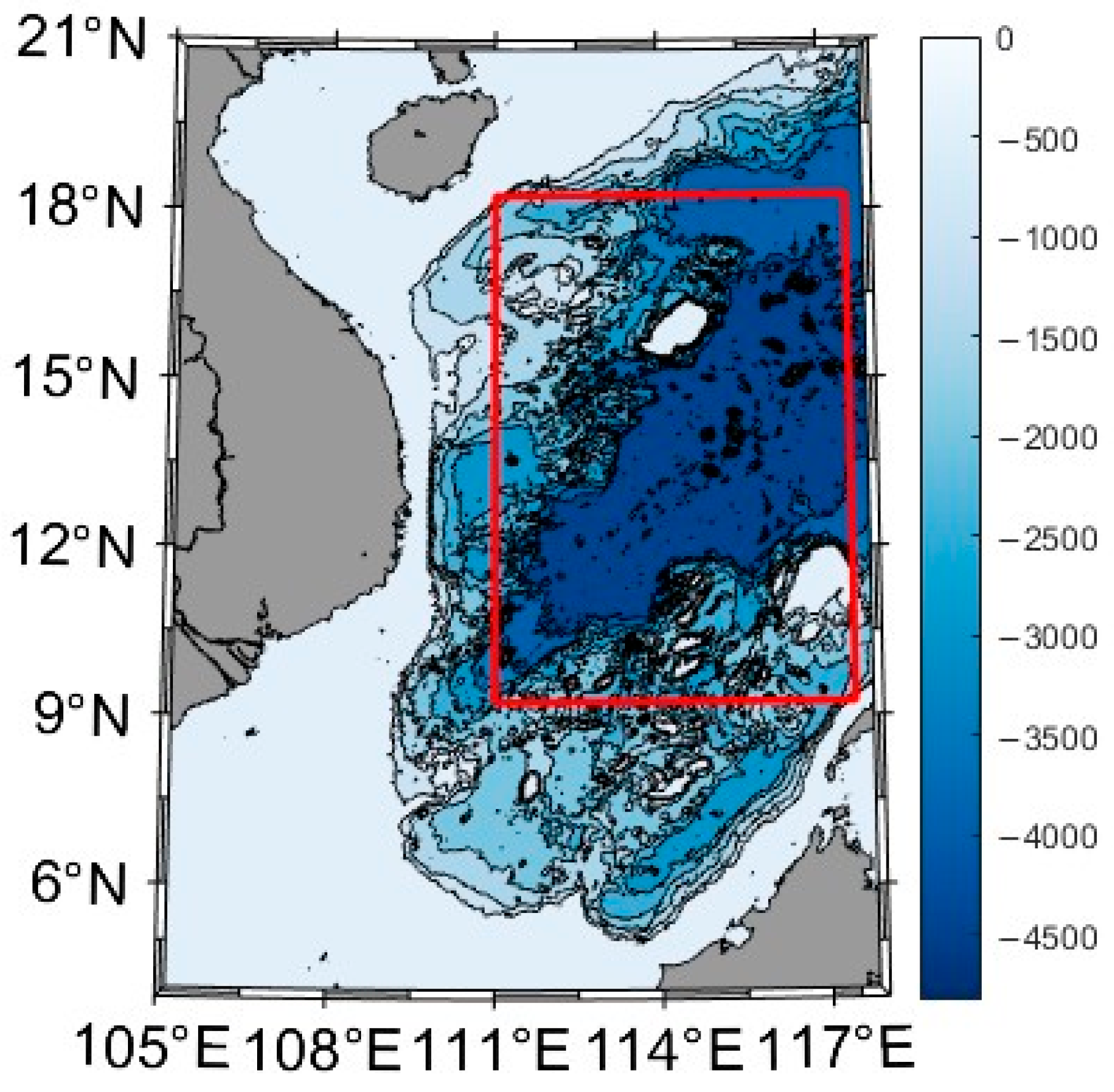
2.1. Materials
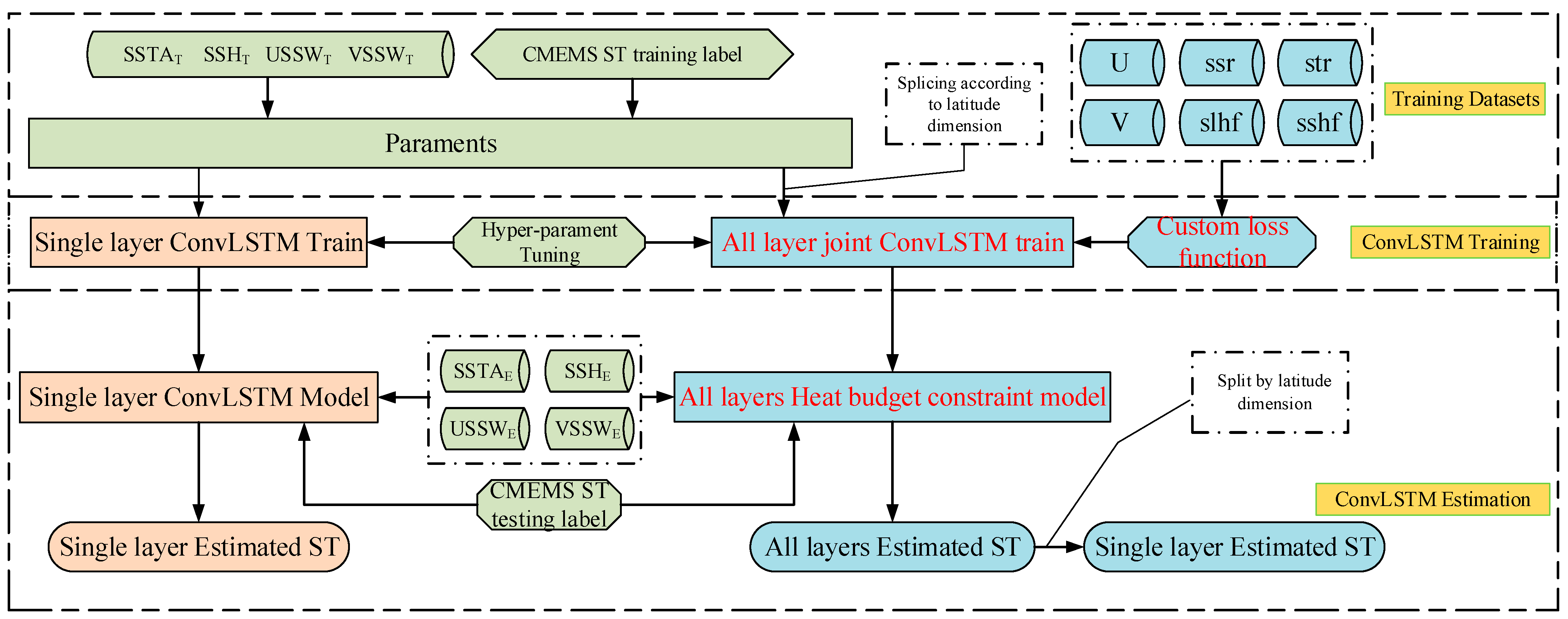
2.2. Methods
2.3. Experimental Setup
3. Results
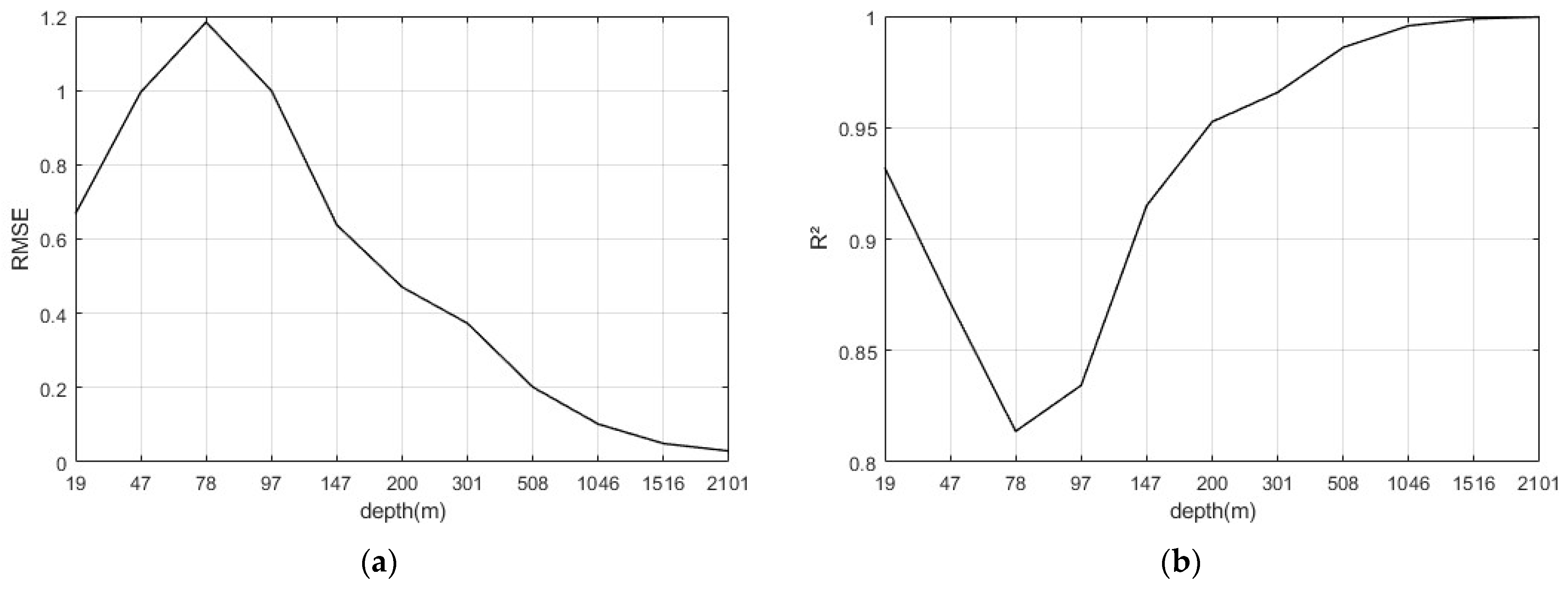
3.1. Results of the Traditional Model
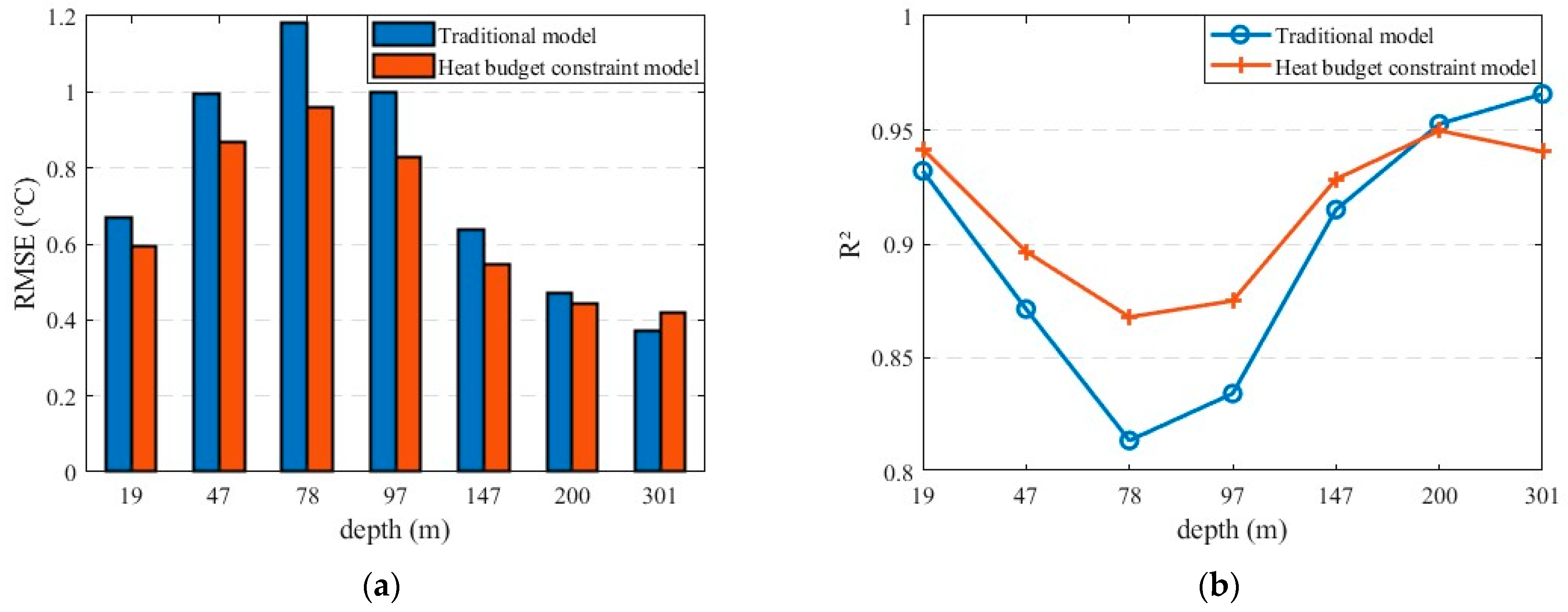
3.2. Results of the Heat Budget Constraint Model
4. Discussion
4.1. A Comparison of the Performance of the Heat Budget Constraint Model Method with the Research Results of Others
4.2. The Influence of the Randomness of the Dataset Division on the Results
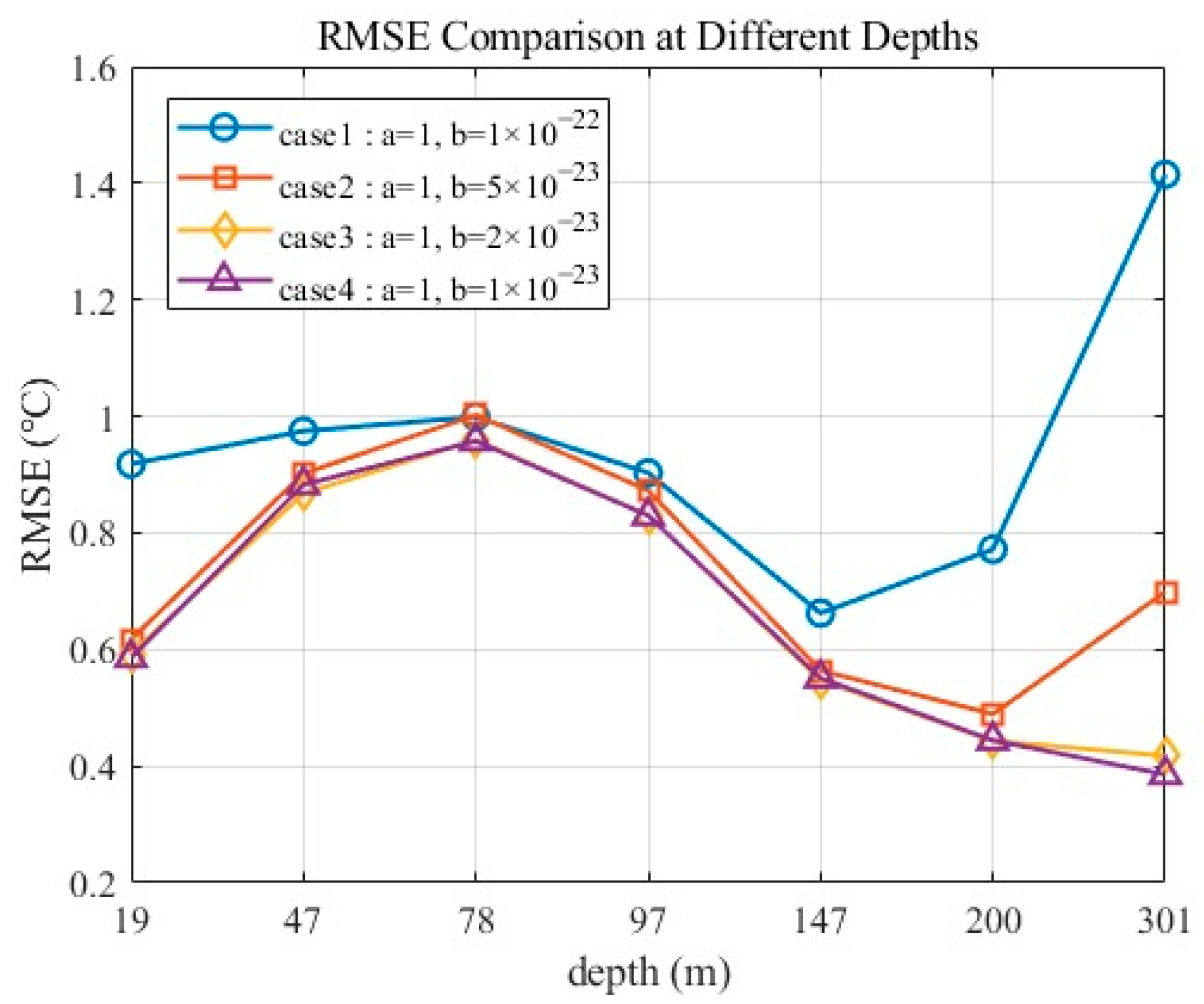
4.3. The Influence of the Selection of the Weighting Coefficient in the Loss Function on the Model Accuracy
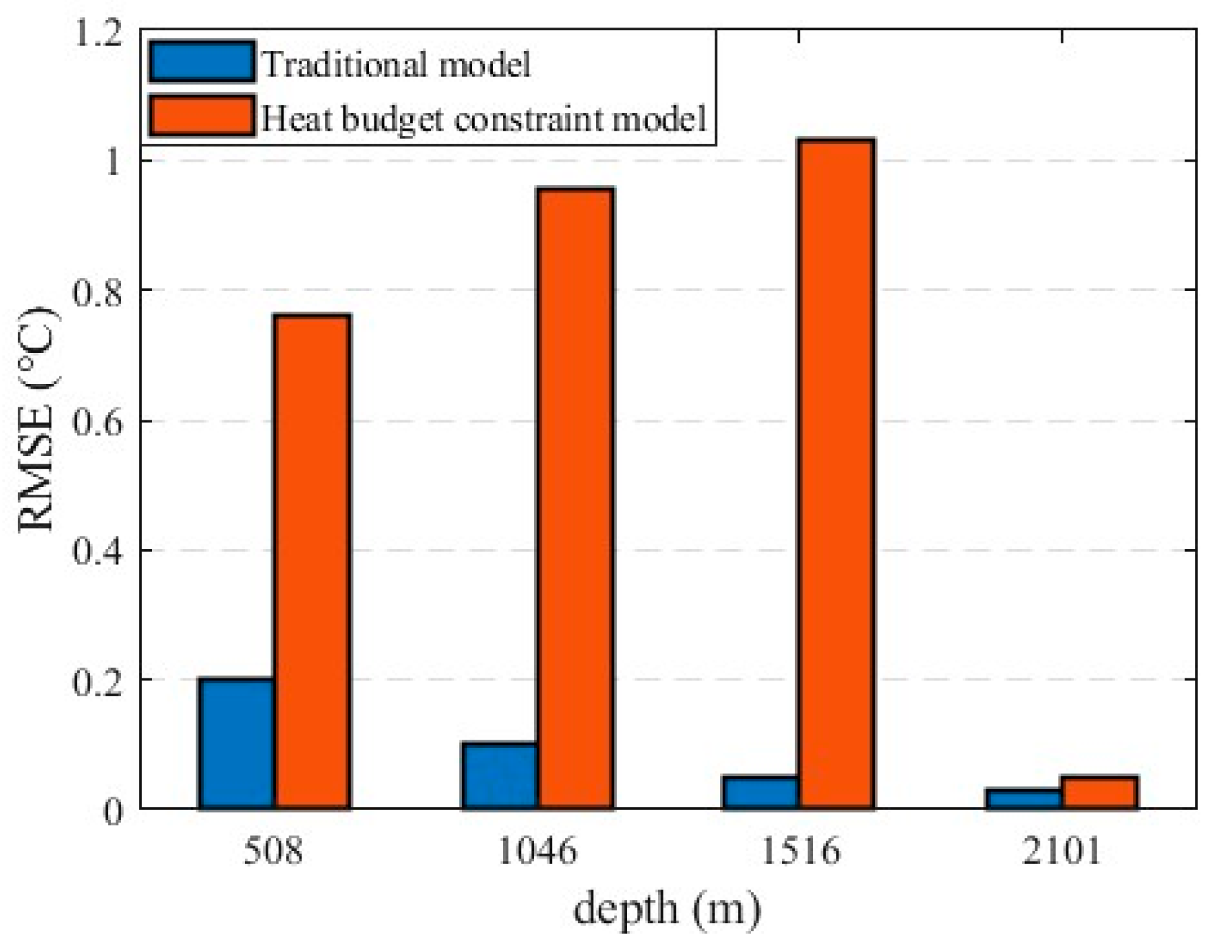
4.4. The Analysis of the Reasons for the Failure of the Heat Budget Constraint Model in the Deep Sea Ocean
5. Conclusions
Author Contributions
Funding
Data Availability Statement
Conflicts of Interest
References
- Klemas, V.; Yan, X.H. Subsurface and Deeper Ocean Remote Sensing from Satellites: An Overview and New Results. Prog. Oceanogr. 2014, 122, 1–9. [Google Scholar] [CrossRef]
- Li, X.; Liu, B.; Zheng, G.; Ren, Y.; Zhang, S.; Liu, Y.; Gao, L.; Liu, Y.; Zhang, B.; Wang, F. Deep-Learning-Based Information Mining from Ocean Remote-Sensing Imagery. Natl. Sci. Rev. 2020, 7, 1584–1605. [Google Scholar] [CrossRef] [PubMed]
- Zhang, X.; Li, X.; Zheng, Q. A Machine-Learning Model for Forecasting Internal Wave Propagation in the Andaman Sea. IEEE J. Sel. Top. Appl. Earth Obs. Remote Sens. 2021, 14, 3095–3106. [Google Scholar] [CrossRef]
- Liu, S.Q.; Chen, W.L.; Zhang, M.H.; Chen, L.; Zhang, J.W.; Chen, J.J.; Qin, Y.P.; Wu, S.G. Distribution Characteristics of Planktonic Foraminifera in Surface Sediments of the Zhongsha Area, South China Sea and Their Indicative Significance. Mar. Geol. Front. 2022, 38, 9–25. (In Chinese) [Google Scholar]
- Li, Y.; Li, B.; Li, T. Distribution Characteristics and Influencing Factors of Benthic Foraminifera in Surface Sediments of the Northern South China Sea. Mar. Geol. Front. 2022, 38, 30–36. (In Chinese) [Google Scholar]
- Zhu, H.B.; Fu, T. South China Sea Institute of Oceanology Reveals Mechanisms of Upper Ocean Circulation Changes under Global Warming. China Science Daily, 12 May 2022; 003, (In Chinese). [Google Scholar] [CrossRef]
- Liu, Q.Y. Seasonal and Intraseasonal Variability of Upper Ocean Circulation and Thermal Structure in the South China Sea: Characteristics and Formation Mechanisms; Ocean University of China: Qingdao, China, 2000. (In Chinese) [Google Scholar]
- Wu, D.J. Response and Feedback of Upper Ocean Thermal Structure to Tropical Cyclones. Ph.D. Thesis, First Institute of Oceanography, Ministry of Natural Resources, Qingdao, China, 2024. (In Chinese). [Google Scholar] [CrossRef]
- Wei, Z.X.; Zheng, Q.A.; Yang, Y.Z.; Liu, K.X.; Xv, T.F.; Wang, F.; Hu, S.J.; Xie, L.L.; Li, Y.L.; Du, Y. Seventy Years of Physical Oceanography Research in China: Development History and Academic Achievements. Acta Oceanol. Sin. 2019, 41, 23–64. (In Chinese) [Google Scholar]
- Gao, W.J.; Li, J.; Liu, M.H.; Li, H.; Li, H. Possible Influence of Sea Temperature Changes in the South China Sea and Surrounding Areas on Atmospheric Circulation in Spring. Sci. Technol. Innov. 2023, 13, 156–158. (In Chinese) [Google Scholar] [CrossRef]
- Steinke, S.; Glatz, C.; Mohtadi, M.; Groetneveld, J.; Li, Q.; Jialn, Z. Past Dynamics of the East Asian Monsoon: No Inverse Behaviour Between the Summer and Winter Monsoon During the Holocene. Glob. Planet. Change 2011, 78, 170–177. [Google Scholar] [CrossRef]
- Yokoyama, Y.; Suzuki, A.; Siringan, F.; Maetda, Y.; Albe-Ouchi, A.; Ohgaito, R.; Kawahata, H.; Matsuzaki, H. Mid-Holocene Palaeoceanography of the Northern South China Sea Using Coupled Fossil-Modern Coral and Atmosphere-Ocean GCM Model. Geophys. Res. Lett. 2011, 38, 00F03. [Google Scholar] [CrossRef]
- Mao, Q.W.; Chu, X.Q.; Yan, Y.F.; Qi, Y.Q.; Wang, X.D.; Gong, J.Z.; Cai, D.M.; Wu, Z.D.; Pan, C.M. Design and Implementation of a Three-Dimensional Dynamic Temperature-Salinity Field Reconstruction System for the South China Sea. J. Trop. Oceanogr. 2013, 32, 1–8. (In Chinese) [Google Scholar]
- Tang, B.; Zhao, D.; Cui, C.; Zhao, X. Reconstruction of Ocean Temperature and Salinity Profiles in the Northern South China Sea Using Satellite Observations. Front. Mar. Sci. 2022, 9, 945835. [Google Scholar] [CrossRef]
- Qi, J.; Liu, C.; Chi, J.; Li, D.; Gao, L.; Yin, B. An Ensemble-Based Machine Learning Model for Estimation of Subsurface Heat Structure in the South China Sea. Remote Sens. 2022, 14, 3207. [Google Scholar] [CrossRef]
- Khedouri, E.; Szczechowski, C.; Cheney, R. Potential Oceanographic Applications of Satellite Altimetry for Inferring Subsurface Heat Structure. In Proceedings of the OCEANS’83, San Francisco, CA, USA, 29 August–1 September 1983; pp. 274–280. [Google Scholar]
- Chu, P.C.; Fan, C.; Liu, W.T. Determination of Vertical Heat Structure from Sea Surface Temperature. J. Atmos. Ocean. Technol. 2000, 17, 971–979. [Google Scholar] [CrossRef]
- Fox, D.N.; Teague, W.J.; Barron, C.N.; Carnes, M.R.; Lee, C.M. The Modular Ocean Data Assimilation System (MODAS). J. Atmos. Ocean. Technol. 2002, 19, 240–252. [Google Scholar] [CrossRef]
- Swart, S.; Speich, S. An Altimetry-Based Gravest Empirical Mode South of Africa: 2. Dynamic Nature of the Antarctic Circumpolar Current Fronts. J. Geophys. Res. Oceans 2010, 115, 03003. [Google Scholar] [CrossRef]
- Meijers, A.J.S.; Bindoff, N.L.; Rintoul, S.R. Estimating the Four-Dimensional Structure of the Southern Ocean Using Satellite Altimetry. J. Atmos. Ocean. Technol. 2011, 28, 548–568. [Google Scholar] [CrossRef]
- Ali, M.M.; Swain, D.; Weller, R.A. Estimation of Ocean Subsurface Heat Structure from Surface Parameters: A Neural Network Approach. Geophys. Res. Lett. 2004, 31, 20308. [Google Scholar] [CrossRef]
- Su, H.; Zhang, H.; Geng, X.; Qin, T.; Lu, W.; Yan, X.H. OPEN: A New Estimation of Global Ocean Heat Content for Upper 2000 Meters from Remote Sensing Data. Remote Sens. 2020, 12, 2294. [Google Scholar] [CrossRef]
- Su, H.; Li, W.; Yan, X.-H. Retrieving Temperature Anomaly in the Global Subsurface and Deeper Ocean from Satellite Observations. J. Geophys. Res. Oceans 2018, 123, 399–410. [Google Scholar] [CrossRef]
- Lu, W.; Su, H.; Yang, X.; Yan, X.-H. Subsurface Temperature Estimation from Remote Sensing Data Using a Clustering-Neural Network Method. Remote Sens. Environ. 2019, 229, 213–222. [Google Scholar] [CrossRef]
- Su, H.; Yang, X.; Lu, W.; Yan, X.-H. Estimating Subsurface Thermohaline Structure of the Global Ocean Using Surface Remote Sensing Observations. Remote Sens. 2019, 11, 1598. [Google Scholar] [CrossRef]
- Su, H.; Zhang, T.; Lin, M.; Lu, W.; Yan, X.-H. Predicting Subsurface Thermohaline Structure from Remote Sensing Data Based on Long Short-Term Memory Neural Networks. Remote Sens. Environ. 2021, 260, 112465. [Google Scholar] [CrossRef]
- Cheng, H.; Sun, L.; Li, J. Neural Network Approach to Retrieving Ocean Subsurface Temperatures from Surface Parameters Observed by Satellites. Water 2021, 13, 388. [Google Scholar] [CrossRef]
- Han, M.; Feng, Y.; Zhao, X.; Sun, C.; Hong, F.; Liu, C. A Convolutional Neural Network Using Surface Data to Predict Subsurface Temperatures in the Pacific Ocean. IEEE Access 2019, 7, 172816–172829. [Google Scholar] [CrossRef]
- Shi, X.; Chen, Z.; Wang, H.; Yeung, D.Y.; Wong, W.K.; Woo, W.C. Convolutional LSTM Network: A Machine Learning Approach for Precipitation Nowcasting. Adv. Neural Inf. Process. Syst. 2015, 28, 802–810. [Google Scholar]
- Song, T.; Wei, W.; Meng, F.; Wang, J.; Han, R.; Xu, D. Inversion of Ocean Subsurface Temperature and Salinity Fields Based on Spatio-Temporal Correlation. Remote Sens. 2022, 14, 2587. [Google Scholar] [CrossRef]
- Song, T.; Xu, G.; Yang, K.; Li, X.; Peng, S. Convformer: A Model for Reconstructing Ocean Subsurface Temperature and Salinity Fields Based on Multi-Source Remote Sensing Observations. Remote Sens. 2024, 16, 2422. [Google Scholar] [CrossRef]
- Zhang, Y.; Liu, Y.; Kong, Y.; Hu, P. An Improved Method for Retrieving Subsurface Temperature Using the ConvLSTM Model in the Western Pacific Ocean. J. Mar. Sci. Eng. 2024, 12, 620. [Google Scholar] [CrossRef]
- Luo, C.; Huang, M.; Guan, S.; Zhao, W.; Tian, F.; Yang, Y. Subsurface Temperature and Salinity Structures Inversion Using a Stacking-Based Fusion Model from Satellite Observations in the South China Sea. Adv. Atmos. Sci. 2025, 42, 204–220. [Google Scholar] [CrossRef]


| Input Variable | Dataset | Source |
|---|---|---|
| SSH | AVISO | https://www.aviso.altimetry.fr/en/data.html (accessed on 29 December 2023) |
| SST | OISST | https://www.ncei.noaa.gov/thredds/blended-global/oisst-catalog.html (accessed on 29 December 2023) |
| USSW, VSSW | CCMP | https://rda.ucar.edu/datasets/d745001/dataaccess/ (accessed on 29 December 2023) |
| ST | CMEMS | https://data.marine.copernicus.eu/products (accessed on 29 April 2024) |
| slhf, ssr, str, sshf | ERA5 | https://cds.climate.copernicus.eu/datasets/reanalysis-era5-single-levels%3Ftab%3Dform?tab=download (accessed on 24 June 2024) |
| U, V | CMEMS | https://data.marine.copernicus.eu/products (accessed on 16 August 2024) |
| Hyperparameters | Optimal Values | |
|---|---|---|
| Network parameters | num_layers_ConvLSTM2D | 2 |
| kernel_size_ConvLSTM2D | 3 × 3 | |
| activation_ConvLSTM2D | Relu | |
| num_layers_Conv3D | 1 | |
| kernel_size_Conv3D | 3 × 3 × 3 | |
| activation_Conv3D | Relu | |
| Optimized parameters | time_step | 3 |
| training_epoch | Customized | |
| learning_rate | 0.001 | |
| optimizer | Adam | |
| Regularization parameter | Dropout | 0.3 |
| 19 m | 47 m | 78 m | 97 m | 147 m | 200 m | 301 m | 508 m | 1046 m | 1516 m | 2101 m | Avg | Avg Above 301 m | |
|---|---|---|---|---|---|---|---|---|---|---|---|---|---|
| Spring | 0.50 | 0.87 | 0.98 | 0.88 | 0.59 | 0.44 | 0.36 | 0.18 | 0.11 | 0.05 | 0.03 | 0.45 | 0.66 |
| Summer | 0.63 | 1.03 | 1.01 | 0.91 | 0.55 | 0.40 | 0.31 | 0.18 | 0.10 | 0.05 | 0.03 | 0.48 | 0.69 |
| Autumn | 0.59 | 1.00 | 1.23 | 0.99 | 0.63 | 0.48 | 0.40 | 0.20 | 0.09 | 0.04 | 0.02 | 0.52 | 0.76 |
| Winter | 0.75 | 0.97 | 1.20 | 1.04 | 0.68 | 0.52 | 0.39 | 0.19 | 0.08 | 0.04 | 0.02 | 0.54 | 0.79 |
| Spring | 0.96 | 0.89 | 0.84 | 0.84 | 0.92 | 0.96 | 0.97 | 0.99 | 0.99 | 0.99 | 0.99 | 0.94 | 0.91 |
| Summer | 0.93 | 0.87 | 0.84 | 0.86 | 0.93 | 0.97 | 0.97 | 0.99 | 0.99 | 0.99 | 0.99 | 0.94 | 0.91 |
| Autumn | 0.94 | 0.86 | 0.80 | 0.83 | 0.91 | 0.95 | 0.96 | 0.99 | 0.99 | 0.99 | 0.99 | 0.93 | 0.89 |
| Winter | 0.90 | 0.86 | 0.79 | 0.81 | 0.90 | 0.94 | 0.96 | 0.99 | 0.99 | 0.99 | 0.99 | 0.92 | 0.88 |
| 19 m | 47 m | 78 m | 97 m | 147 m | 200 m | 301 m | Avg Above 301 m | |
|---|---|---|---|---|---|---|---|---|
| Spring | 0.586 | 0.699 | 0.743 | 0.712 | 0.515 | 0.406 | 0.375 | 0.577 |
| Summer | 0.527 | 0.884 | 0.935 | 0.805 | 0.519 | 0.427 | 0.420 | 0.645 |
| Autumn | 0.580 | 0.91 | 1.005 | 0.841 | 0.548 | 0.435 | 0.373 | 0.670 |
| Winter | 0.529 | 0.744 | 0.986 | 0.842 | 0.530 | 0.423 | 0.384 | 0.634 |
| Spring | 0.935 | 0.920 | 0.900 | 0.893 | 0.931 | 0.954 | 0.945 | 0.925 |
| Summer | 0.945 | 0.890 | 0.871 | 0.878 | 0.922 | 0.948 | 0.928 | 0.912 |
| Autumn | 0.936 | 0.880 | 0.856 | 0.867 | 0.922 | 0.947 | 0.948 | 0.908 |
| Winter | 0.945 | 0.911 | 0.845 | 0.863 | 0.927 | 0.951 | 0.946 | 0.913 |
Disclaimer/Publisher’s Note: The statements, opinions and data contained in all publications are solely those of the individual author(s) and contributor(s) and not of MDPI and/or the editor(s). MDPI and/or the editor(s) disclaim responsibility for any injury to people or property resulting from any ideas, methods, instructions or products referred to in the content. |
© 2025 by the authors. Licensee MDPI, Basel, Switzerland. This article is an open access article distributed under the terms and conditions of the Creative Commons Attribution (CC BY) license (https://creativecommons.org/licenses/by/4.0/).
Share and Cite
Xu, D.; Liu, Y.; Kong, Y. A Deep Learning Inversion Method for 3D Temperature Structures in the South China Sea with Physical Constraints. J. Mar. Sci. Eng. 2025, 13, 1061. https://doi.org/10.3390/jmse13061061
Xu D, Liu Y, Kong Y. A Deep Learning Inversion Method for 3D Temperature Structures in the South China Sea with Physical Constraints. Journal of Marine Science and Engineering. 2025; 13(6):1061. https://doi.org/10.3390/jmse13061061
Chicago/Turabian StyleXu, Dongcan, Yahao Liu, and Yuan Kong. 2025. "A Deep Learning Inversion Method for 3D Temperature Structures in the South China Sea with Physical Constraints" Journal of Marine Science and Engineering 13, no. 6: 1061. https://doi.org/10.3390/jmse13061061
APA StyleXu, D., Liu, Y., & Kong, Y. (2025). A Deep Learning Inversion Method for 3D Temperature Structures in the South China Sea with Physical Constraints. Journal of Marine Science and Engineering, 13(6), 1061. https://doi.org/10.3390/jmse13061061