The Spatial–Temporal Characteristics of Wave Energy Resource Availability in the China Seas

Abstract

For coastal nations and regions, wave energy provides a localized energy solution, decreasing dependency on external energy sources and fostering the sustainable development of local economies. Effective wave height occurrence (EWHO) represents the availability of wave energy and is a crucial parameter for site selection for optimal wave energy. This paper systematically analyzes the distribution of EWHO in China seas areas using significant wave height (SWH) data in the fifth generation of ECMWF atmospheric reanalysis (ERA5) and key climate indices. Employing methods such as climate statistical analysis, linear regression, significance testing, and trend analysis, the study highlights the temporal and spatial distribution characteristics, variation trends, and correlations with climate indices of EWHO. This research aims to provide technical assistance and decision support for the development of wave energy at sea. The results indicate the following conclusions: (1) The high EWHO in the China seas is predominantly located in northern Nanhai, southern Donghai, and the eastern waters of the Philippine Islands. The EWHO is highest in winter. (2) The growth trend of EWHO is most notable in the sea area east of the line connecting the Ryukyu Islands, Taiwan, and the northeastern Philippines, peaking in spring and being relatively weak in winter. (3) The correlation between NINO3 and EWHO is most significant in Nanhai and the northeastern waters of the Philippines, peaking in February with correlation coefficients ranging from −0.30 to −0.50.

1. Introduction

The area of Chinese maritime territory exceeds 3 million km². Coastal regions in China are highly developed, accounting for approximately 70% of national Gross Domestic Product (GDP). Consequently, these coastal regions account for over 50% of China’s total electricity consumption. The availability of energy represents a critical factor limiting the development of these coastal regions. As an important source of renewable energy, there is a critical need for further study on how to effectively utilize wave energy in the China seas. Effective wave height occurrence (EWHO) represents the availability of wave energy and is a crucial parameter for site selection for optimal wave energy. EWHO directly reflects the proportion of the year during which wave energy can be harnessed, which is essential for ensuring the stable supply and development of wave energy. Although some regions exhibit a relatively high annual average wave energy flux density, significant temporal variations in its distribution can lead to periods of insufficient energy supply. EWHO effectively indicates the proportion of the year when wave energy is exploitable, thereby mitigating this issue and ensuring continuous wave energy output. Additionally, in certain areas, excessively high wave energy flux density might damage wave energy generation devices, hindering wave energy development. Knowledge of EWHO can effectively prevent such situations. Understanding its distribution and trends can provide valuable insights for the effective development of wave energy resources.

Most existing studies on wave energy utilization have focused on patterns in wave energy density and wave height. A study by Zheng et al. [1] utilized the ERA5 dataset to analyze global wave trends and identified global significant wave height (SWH) to be increasing by 0.32 cm/yr, with that in the Southern Hemisphere exceeding that in the Northern Hemisphere. Using ERA-Interim reanalysis data, Wan et al. [2] determined coastal areas to be less affected by severe sea states relative to offshore regions, with the highest and lowest abundance of wave energy being in winter and summer, respectively. A study by Wan et al. [3] utilizing ERA-Interim reanalysis data identified the Northwest Pacific Ocean to have a relatively small area of low wave energy, concentrated in the Bohai Sea and waters around Malaysia; areas of abundant wave energy were extensive, accounting for around 70% of the total oceanic area. Iglesias and Carballo [4] proposed that the required specific percentage of energy coverage is dependent on the variability in regional offshore wave climate, water depth, and coastline shape and orientation. Iglesias et al. [5] identified the highest wave heights in La Palma to occur in winter, followed by autumn, with those in spring and summer being substantially lower; waves generated in the northwest were higher, which they attributed to the extended fetch of oceanic winds in these directions. Iglesias et al. [6] highlighted the potential for wave energy to meet nearly half of the energy requirements of China. There is significant regional variation in maritime wave energy resources, and upward trends in these resources have been observed in some regions. An extensive long-term analysis of the wave energy potential in the Black Sea using 31 years of Simulating Waves Nearshore (SWAN) model simulation data by Akipnar et al. [7] found that December–January–February (DJF) contributed most significantly to the annual average wave power, with a peak of 10.5 kW/m, followed by September–October–November (SON) and March–April–May (MAM), whereas June–July–August (JJA) exhibited the lowest wave power, reaching only 2.3 kW/m. Liang et al. [8] applied wind data from ERA-Interim, the Holland model, and a hybrid model to the SWAN model to simulate wave parameters in Nanhai and Donghai during tropical cyclones. Wave height and period simulated by the hybrid B-S model exhibited greater consistency with observed data. An analysis of the ERA-40 dataset by Semedo et al. [9] identified a significant rise in sea levels (1.2–2.0 cm/yr) from 1957 to 2002 in most parts of the North Pacific and North Atlantic; an analysis of a 57-year forecast obtained through spectral wave models by Dodet et al. [10] identified a significant increase in significant wave height (SWH) in the northern latitudes of the Northeast Atlantic between 1953 and 2009, at a rate of 2.0 cm/yr. The North Atlantic Oscillation (NAO) shows positive and negative correlations with Hs at northern and southern latitudes, respectively; using buoy data, Gower et al. [11] identified an increase in Hs in the Northeast Pacific by approximately 1–4 cm/yr between 1977 and 1999. An analysis of global changes in wind speed (WS) and Hs between 1971 and 2000 by Sterl and Caires [12] using the 45-year European Centre for Medium-Range Weather Forecasts (ECMWF) reanalysis (ERA-40) identified a maximum increase in average Hs of around 4 cm/yr and an average in global ocean WS of 6 cm/s/yr. Using International Comprehensive Ocean-Atmosphere Data Set (ICOADS) data for 1964–1993, Gulev et al. [13] identified an increase in Hs across the North Atlantic of 10–30 cm per decade. A study by Gupta et al. [14], utilizing daily wind and wave data from eight satellite missions for 1992–2012, identified steady increases in maximum Hs and WS in the Southern Ocean of 7.2 cm/yr and 12 cm/s/yr, respectively, and the northward propagation of high waves generated in the Southern Ocean. Using a 31-year long-term wave dataset generated through a three-layer nested modeling system, Akpınar et al. [15] identified minimal fluctuations in mean wave power at stations throughout the day, minimal variation in mean wave power between stations in the summer months, and greater variations between the stations in the winter months. Liang et al. [16] applied the Simulated Waves Nearshore model to simulate wave conditions from 1990 to 2011, with the simulation accuracy validated by observational data and simulations showing the largest and mean significant wave heights and seasonal variations in the largest significant wave height. Zheng et al. [17] identified the calculation results of the global multi-year average WPD over the past 38 years, showing that the high-GWA areas are mainly distributed in the east–west band-like regions of the westerlies in the Southern Hemisphere (>800 W/m²) and the westerlies in the Northern Hemisphere (>600 W/m²). Zheng et al. [18] identified that Nanhai had the highest proportion of exploitable wave energy, exceeding 66%, making it the most suitable sea area for establishing nearshore wave energy power stations. Falnes J [19] identified that wind waves grow driven by the local wind, and that their direction is consistent with or close to the wind direction. Surge waves are long-period waves that propagate from storm areas with little energy loss. Bertin X [20] identified that the increase in significant wave height (Hs) was attributed to the intensification caused by more frequent and stronger storms, as well as greenhouse gas forcing. Islek et al. [21] analyzed ERA-Interim data and integrated long-term stable wind conditions with their study region’s strong wind climate, concluding that the southwestern part of the Black Sea possessed reliable, persistent, and sustainable wind energy potential. Akpınar et al. [22] demonstrated that the mean values of Hm0 and WS in the Black Sea exhibited minimal, almost negligible, variation over different periods. However, the maximum values of Hm0 and WS showed significant changes. Buşra Başaran et al. [23] demonstrated that long-term changes in the wave climate of the Black Sea have led to shifts in spatial and temporal scales in coastal areas, resulting in alterations to coastal morphology. Zhang Xudong et al. [24] performed a comprehensive analysis of the temporal and spatial distribution of wind speed and significant wave height (SWH) in the MSR region. The results indicated that seasonal variations were particularly noticeable in the Luzon Strait and the Gulf of Aden, whereas the central Indian Ocean exhibited relatively stable characteristics. W. Han et al. [25] conducted an analysis of multi-satellite grid data to investigate the probability distribution characteristics of significant wave heights in the Chinese sea area. Their findings indicated that the probability of wave heights ranging from 0.4 m to 1.8 m exceeded 70%, with the highest probability observed for wave heights within the range of 0.6 m to 3 m. Additionally, the probability of the significant wave height (SWH) exceeding 4 m was found to be less than 0.18%. Wang Yanping et al. [26] conducted a study on the long-term changes in wave characteristics caused by storm surges in the Bohai Sea region and found that the extreme values of significant wave height (SWH) at most coastal stations showed a negative trend, with a maximum negative trend of −0.03 m per year in the western part of the Liaodong Bay.

Current research on evaluation indicators for wave energy is still lacking. This paper defines an indicator to assess the utilization rate of wave energy and analyzes the correlation between climate indices and EWHO. The available wave height is defined as a significant wave height (SWH) ranging from 1.3 to 4.0 m [26]. By statistically analyzing the frequency of occurrence of the available wave heights, EWHO data for China sea areas are obtained. Mechanism and trend analyses are conducted, and key climate indices and their correlations are calculated. This study aims to estimate the utilization rate of wave energy in the China seas areas, evaluate wave energy based on changes in climate indices, understand the evolution patterns of wave energy, and provide key recommendations for the site selection of wave energy power plants.

2. Data and Methodology

2.1. Data

Two main types of data are available to investigate trends in EWHO and SWH in the China seas: numerical model outputs and satellite data. The choice of data source can significantly impact the conclusions drawn. Given the focus of the current study on annual and monthly variations in EWHO and SWH, model data were the only viable source. Rapid advancements in observational techniques, numerical simulation methods, and data assimilation approaches have increasingly allowed for the integration of in situ and satellite observations into model reanalysis datasets. The fifth generation of ECMWF reanalysis (ERA5), which succeeded ERA-Interim, is now the most widely adopted dataset for global climate and weather research. This dataset was produced using four-dimensional variational data assimilation (4D-Var) technology, integrating various observational sources, including satellite remote sensing and buoy observations, to ensure high-quality and consistent wave data. The present study selected the ERA5 reanalysis dataset encompassing SWH from 1 January 1940 to 1 January 2022, with temporal and spatial resolutions of 1 h and 0.25° × 0.25°, respectively. Within the seasonal analysis, MAM, JJA, SON, and DJF represent March–April–May, June–July–August, September–October–November, and December–January–February, respectively. The computational area was from 90° E to 140° E and from 0° to 40° N.

2.2. Methodology

The present study used the ERA5 reanalysis dataset to calculate and analyze long-term trends in EWHO and SWH in the China seas over the last 83 years (1940–2022), including overall, seasonal, and regional trends, as well as correlations between EWHO and climate indices. The present study also examined the physical mechanisms responsible for the long-term trends in EWHO. (1) Linear regression and Linear Regression Trend Test were used to calculate the overall trends in EWHO and SWH in the China seas for 1940–2022. (2) A 3-point moving average was applied before calculating the annual trends of the EWHO at each 0.25° × 0.25° grid point for 1940–2022 to analyze regional differences. (3) Monthly trends were statistically analyzed to identify long-term monthly variations. (4) Annual and monthly trends were compared to identify the dominant month of variation. (5) Correlations between the EWHO and climate indices, such as NINO3 and AMOS, were investigated, along with the physical mechanisms responsible for the long-term variations in EWHO.

The steps for using MATLAB (2023a) proceed as follows:

Distribution of EWHO: Utilize MATLAB to count the number of times the SWH falls into the available wave height. Then, calculate the EWHO using Formula (4) and plot the distribution graph of EWHO using the contourf function.

Calculating the rate of change: Calculate the rate of change (slope) of each point in the area by using Equation (2) and determine whether the trend of change is significant based on Equations (4) and (5). Finally, use the contourf function to plot the parts that pass the significance test, and show the areas that fail the test as blank in the graph.

Calculating correlation: Use Formula (6) to calculate the correlation between each point within the region and the climate index, and determine whether the trend of change is significant based on Equations (4) and (5). Finally, use the contourf function to plot the parts that pass the significance test, and show the areas that fail the test as blank in the graph.

Linear regression quantitatively analyzes the linear relationship between two or more variables, revealing the mutual influences among climate factors. The coefficients of the model coefficients can be directly interpreted as the degree of influence one variable has on another.

The equation of linear regression is as follows:

$$Y=\beta +{\beta }_{1}X+\epsilon$$

(1)

In Equation (1), $Y$: dependent variable (value of EWHO); $X$: independent variable (time); $\beta$: intercept (constant term); ${\beta }_1$: regression coefficient (slope: rate of change in EWHO; and $\epsilon$: error term (or residual).

The calculation formula for the slope ${\beta }_1$ is as follows:

$${\beta }_1={\displaystyle \frac{n\sum _{i=1}^n{X}_i{Y}_i+\sum _{i=1}^n{X}_i\sum _{i=1}^n{Y}_i}{n\sum _{i=1}^n{X_i}^2+{\left(\sum _{i=1}^n{X}_i\right)}^2}}$$

(2)

In Equation (2), ${\beta }_1$ represents the slope, $X_i$ is a time series, $Y_i$ is the time series of EWHO, and n is the number of sample points.

The calculation formula for the slope $\beta$ is as follows:

$$\beta ={\displaystyle \frac{\sum _{i=1}^n{Y}_i-{\beta }_1\sum _{i=1}^n{X}_i}{n}}$$

(3)

In Equation (3), $\beta$ is the intercept (constant term), $X_i$ is a time series, $Y_i$ is the time series of EWHO, and n is the number of sample points.

Linear Regression Trend Test: The main advantages of this test were its simplicity, intuitiveness and wide application. It is applicable to data with linear trends and could provide us with clear statistical conclusions, trend directions, and trend magnitudes.

The specific steps were as follows: Hypothesis testing was conducted on the regression coefficient b to calculate the t-statistic. We found the critical value of T for the confidence interval corresponding to the degree of freedom (n − 2) through the T value table. If the T value was greater than the critical T value, it was considered that there was a significant linear relationship in the data.

The calculation formula for the T value is as follows:

$$t={\displaystyle \frac{{\beta }_1}{SE\left({\beta }_1\right)}}$$

(4)

In Equation (3), $SE\left({\beta }_1\right)$ is the error of the regression coefficient and ${\beta }_1$ is the regression coefficient

The calculation formula for SE (${\beta }_1$) is as follows:

$$SE\left(\beta \right)=\sqrt{{\displaystyle \frac{\sum {(Y_i-\widehat{Y_i})}^2}{\left(n-2\right)\sum {(X_i-\overline{X})}^2}}}$$

(5)

In Equation (5), $X_i$ is a time series, $Y_i$ is the time series of EWHO, n is the number of sample points, $\widehat{Y_i}$ is the value of the EWHO time series predicted according to the regression equation, and $\overline{X}$ is the average value of the $X_i$.

The calculation formula for r is as follows:

$$r={\displaystyle \frac{\sum _{i=1}^n{(\mathrm{X}}_i-\overline{X}\left)\right(Y_i-\overline{Y})}{\sqrt{\sum _{i=1}^n{(X_i-\overline{X})}^2\sum _{i=1}^n{(Y_i-\overline{Y})}^2}}}$$

(6)

In Equation (6), $X_i$ is a time series, $Y_i$ is the time series of EWHO, n is the number of sample points, $\overline{X}$ is the average value of the time series $X_i$, and $\overline{Y}$ is the average value of the time series of EWHO.

Zheng et al. [27] identified a significant wave height (SWH) of 1.3–4.0 m to be suitable for wave energy development, whereas an SWH exceeding 4.0 m poses a threat to the operational safety and efficiency of wave energy devices. Therefore, the present study defined an SWH range of 1.3–4.0 m as the wave height suitable for wave energy development (referred to as the available wave height), calculated as follows:

$$\mathrm{E}\mathrm{W}\mathrm{H}\mathrm{O}={\displaystyle \frac{\mathrm{S}\mathrm{W}\mathrm{H}\mathrm{F}}{T}}\times 100\%$$

(7)

In Equation (7), where EWHO is the effective wave height occurrence, SWHF is the number of SWH incidences within the range of 1.3–4.0 m, and T is the annual total number of waves.

3. Regional and Monthly Differences in SWH

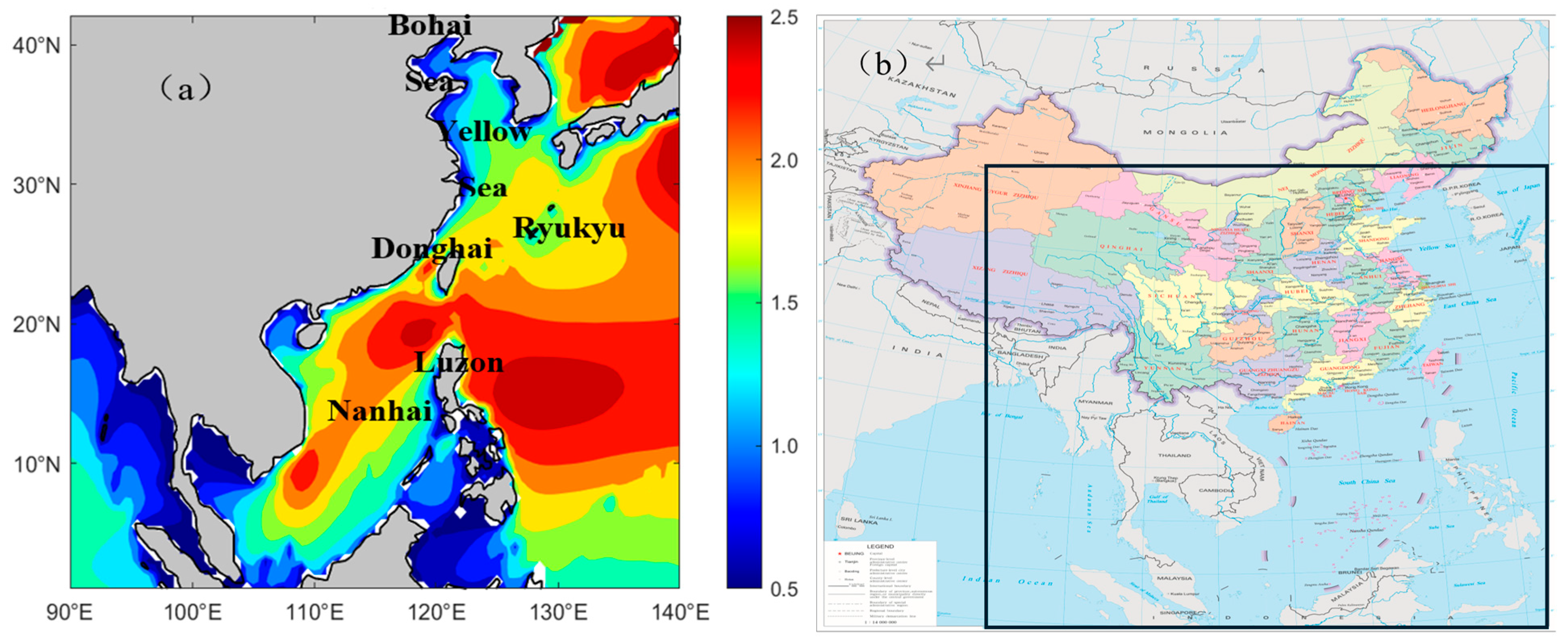
3.1. Regional Differences in Annual Average SWH

The present study analyzed the annual average distribution of SWH in the China seas by calculating the average SWH at each grid point (0.25° × 0.25°) for 1940–2022. Figure 1 shows the significant regional differences in SWH, with a general increase from west to east. Most regions fall within the range of available wave heights, including northern Nanhai, southern Donghai, and the waters east of the Philippines. Notably, higher SWH values are concentrated between the Ryukyu Islands and Luzon Strait and the southeastern area of the Indochina Peninsula, with a northeast–southwest zonal distribution and SWHs between 1.5 and 2.0 m. The highest SWH values in this area were in the Luzon Strait and its adjacent western waters at 1.8–2.5 m. Low SWH values were concentrated in the Bohai Sea and the northern area of the Yellow Sea at <1.0 m.

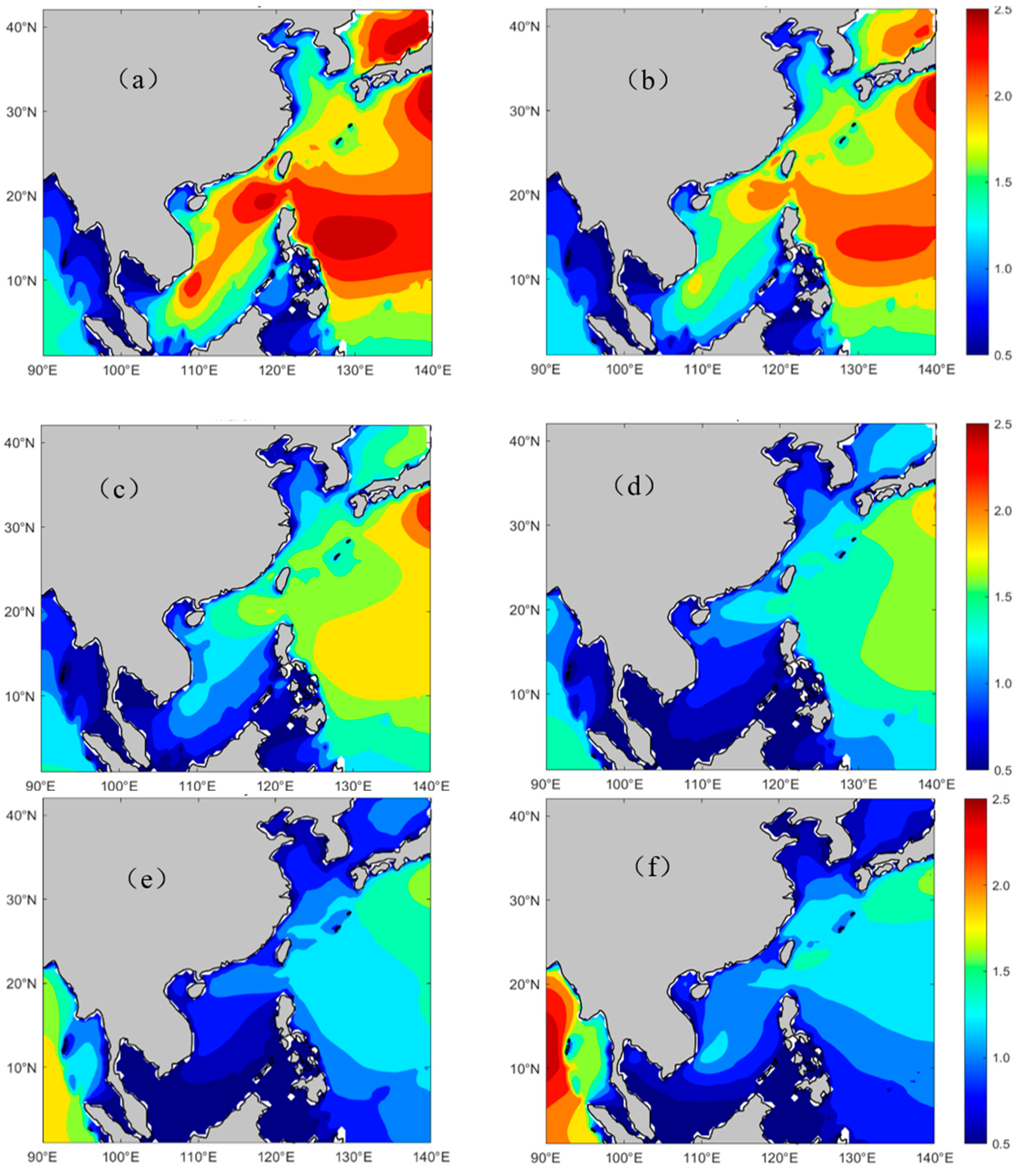
3.2. Monthly Differences in SWH

The present study analyzed the monthly average distribution of the SWH in the China seas by calculating the average SWH at each grid point (0.25° × 0.25°) from January to December for 1940–2022. As shown in Figure 2, there were significant temporal and regional variations in SWH, falling within the range of available wave heights in most regions of the China seas, including northern Nanhai, southern Donghai, and the waters east of the Philippines. The area with SWHs within the range of available wave heights exceeded half of the total area from November to February, peaking in December at over 80%. Further, the SWH exceeded 2.0 m in approximately half of this area during these months. Low SWHs occurred from May to July, with most areas below 1.5 m. The SWH reached its lowest point in May, with more than 90% of the area being below 1.5 m. There were clear seasonal variations in the distribution of SWH in the central and northern regions of Nanhai and the eastern areas near Luzon. The highest SWHs were recorded in DJF (1.7–2.5 m), followed by SON (1.2–2.0 m), MAM (1.0 m–2.5 m), and JJA (0.5–1.2 m). When considering only the annual and monthly mean SWH, there were relatively high and stable annual and monthly averages of SWH in the waters connecting Hainan Island, Taiwan Island, and Luzon Island relative to other offshore areas of China, indicating their suitability for the development of wave energy resources.

4. Regional and Monthly Differences in EWHO

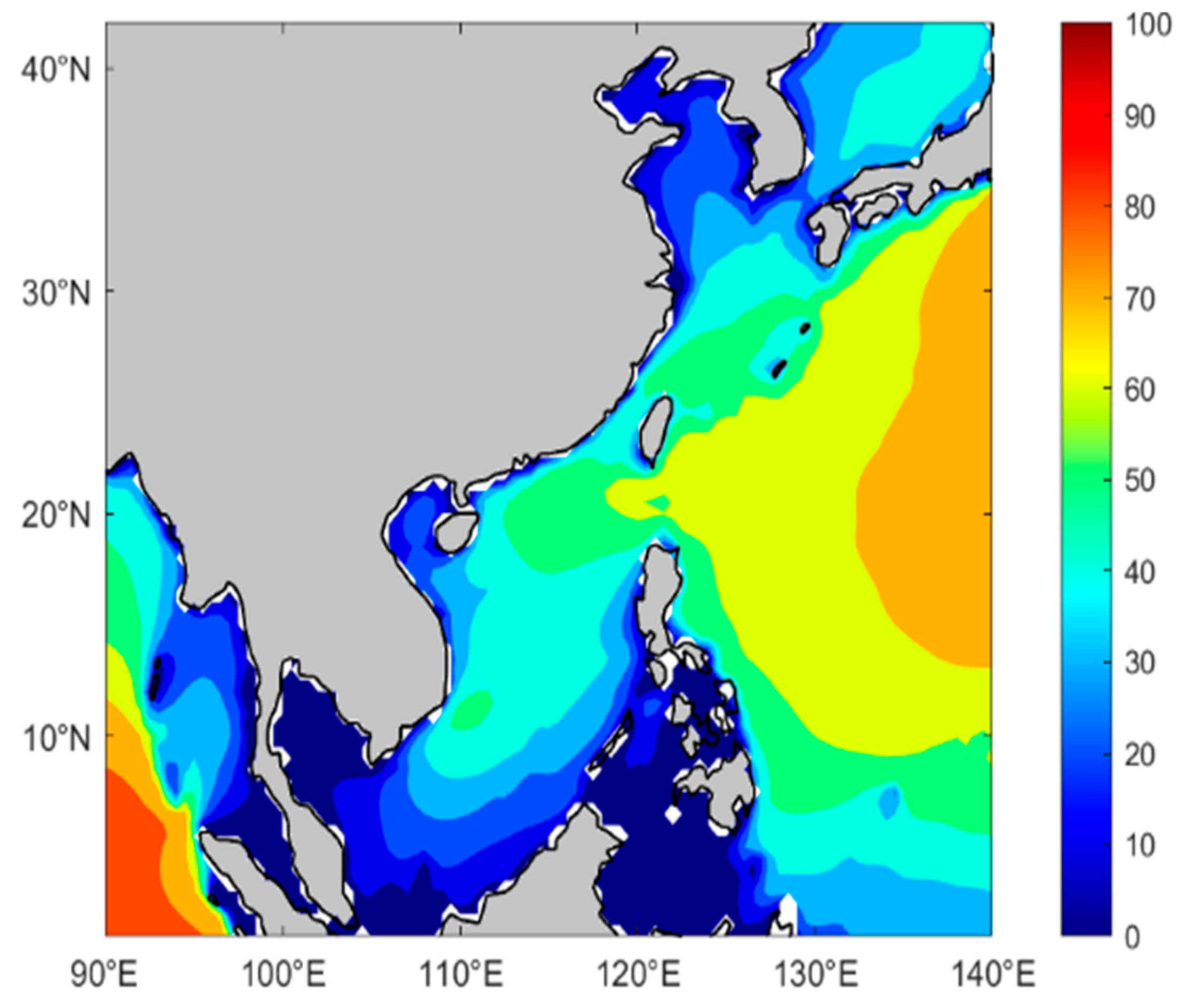
4.1. Regional Differences in Annual Average EWHO

The present study analyzed the annual average distribution of EWHO in the China seas by calculating the average EWHO at each grid point (0.25° × 0.25°) for 1940–2022. As shown in Figure 3, there were significant regional differences in the distribution of EWHO. The EWHO in the China seas ranged from 10% to 70%, with annual averages decreasing from east to west. The area in which EWHO exceeded 50% was the largest in the China seas, concentrated east of the Ryukyu Islands, Taiwan Island, and the Philippines, exhibiting a west-to-east zonal distribution, where the peak EWHO reached approximately 60%. Low EWHO values (below 30%) were identified in the Bohai Sea and the northern Yellow Sea.

However, the regional distribution patterns of EWHO and SWH (significant wave height) differed. High SWHs were concentrated in the Ryukyu Islands–Luzon Strait–southeastern Indochina Peninsula area, with a northeast–southwest zonal distribution, whereas higher EWHOs were concentrated east of the Ryukyu Islands, Taiwan Island, and the Philippines, showing a west-to-east zonal distribution. The peak EWHO occurred in the eastern waters, while the peak SWH appeared in the Luzon Strait and adjacent western waters. Given these regional disparities, understanding EWHO distribution is crucial for effective wave energy development and utilization.

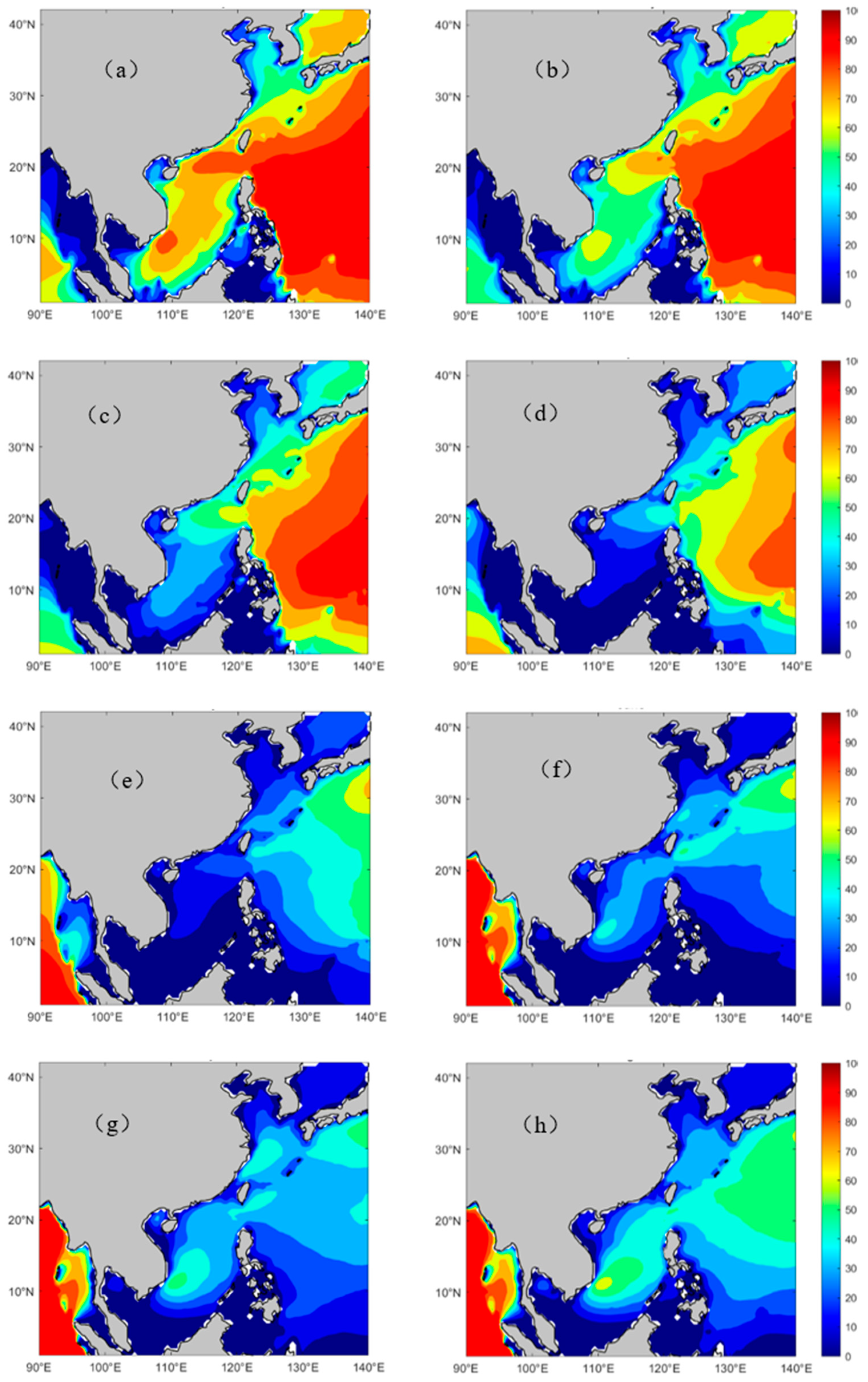
4.2. Monthly Differences in EWHO

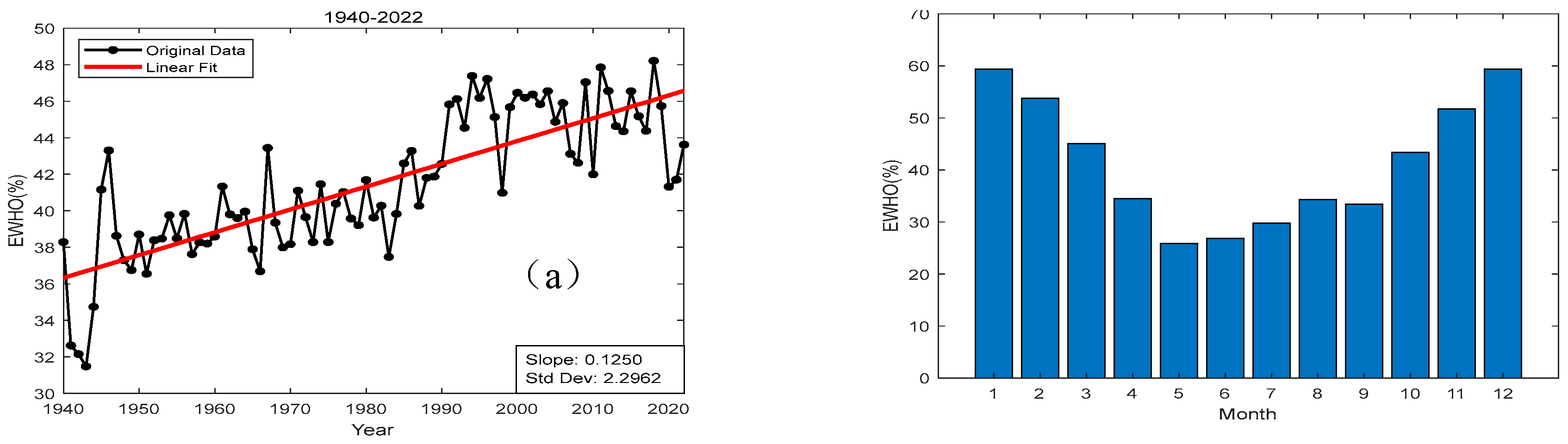
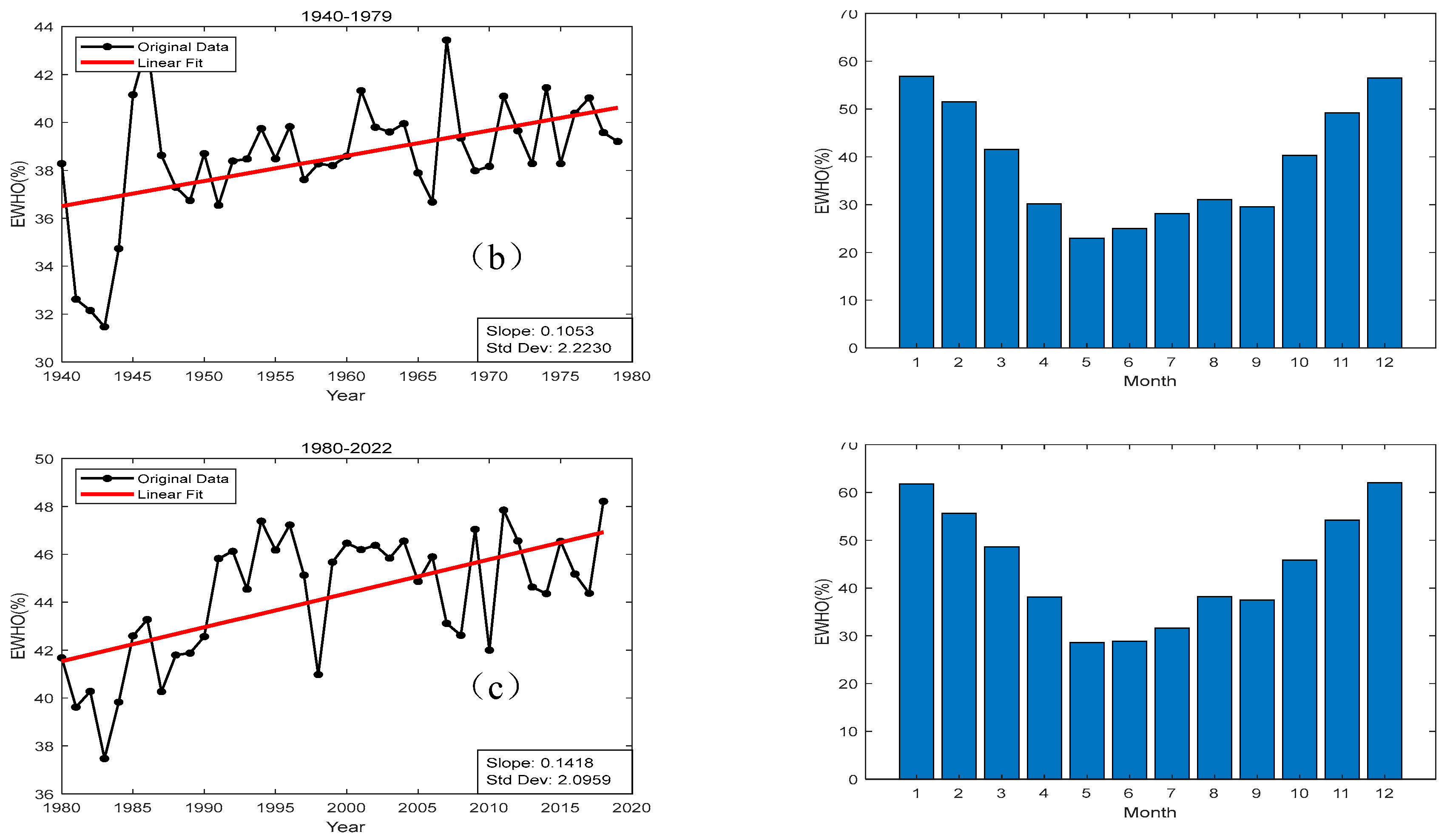
The present study analyzed the monthly average distribution of EWHO in the China seas by calculating the average EWHO at each grid point (0.25° × 0.25°) from January to December for 1940–2022. As shown in Figure 4, there were significant regional and temporal differences in EWHO from January to December. Higher EWHO values were observed from November to February, exceeding 50% in most areas, and the peak EWHO was in December, reaching 70% in most regions. Conversely, low EWHO values were observed from May to July, below 50% in most regions, and the lowest EWHO was observed in May, during which the EWHO was below 40% in more than half of the region.

There were significant differences in the annual distributions of EWHO and SWH in Nanhai and the eastern coast of the Philippines. Although SWH was generally high in this area, there was a significant decrease in the spatial extent of high values of EWHO. This pattern could be mainly attributed to the higher SWH values in this region from November to January compared to those in other regions, exceeding the range of available wave heights. This in turn resulted in a decline in EWHO. Although SWH also increased in other regions, initially low values of SWH resulted in increased instances of SWH within the range of usable wave height, leading to an increase in EWHO. These factors contributed to the differences in regional distributions between EWHO and SWH. Concurrently, Nanhai and the eastern Philippines exhibited significantly higher SWH relative to those of other regions during January, November, and December. This in turn resulted in a higher annual average SWH, thereby exacerbating regional disparities in the annual distributions of SWH and EWHO.

5. Trends in EWHO

5.1. Overall Variation

The present study analyzed temporal variations in EWHO by calculating both the annual average and January–December average EWHO for each grid point (0.25° × 0.25°) for 1940–2022. These averages were then aggregated by region, as illustrated in Figure 5 and Figure 6. As shown in Figure 5a, EWHO showed an increasing linear trend with time, with a correlation coefficient (R) of 0.63, significant at the 99% level. A significant increasing trend in EWHO of 0.13%/yr in the China seas for 1940–2022 was identified. The lowest EWHO occurred in 1943, whereas it increased at a rate of 0.11%/yr. from 1940 to 1979, and then at a rate of 0.14%/yr from 1980 to 2022. The drop in EWHO in the China seas in 1998 could be attributed to a strong El Niño event which occurred from April 1997 to May 1998 along with a weakened East-Asian Monsoon. A V-shaped pattern in the annual distribution of the EWHO was evident, with higher EWHO at the beginning and end of the year and low values in the middle. Within the year, periods of high EWHO were concentrated in January to February and November to December, whereas low EWHO values occurred from May to July, with the highest and lowest EWHO being found in January and May, respectively.

There was an overall increasing trend in EWHO in the China seas from January to December. Within this inter-annual increasing trend, there were clear seasonal patterns in EWHO, with higher rates of increase from January to May and from August to December, with particularly notable growth rates of 0.19%/yr in April and 0.11%/yr in December. Conversely, EWHO remained relatively stable from June to July. High EWHO values were primarily observed between January and March and between November and December, consistently exceeding 65% in recent years. Low values of EWHO, consistently near 40% in recent years, were mainly concentrated in May, June, and September.

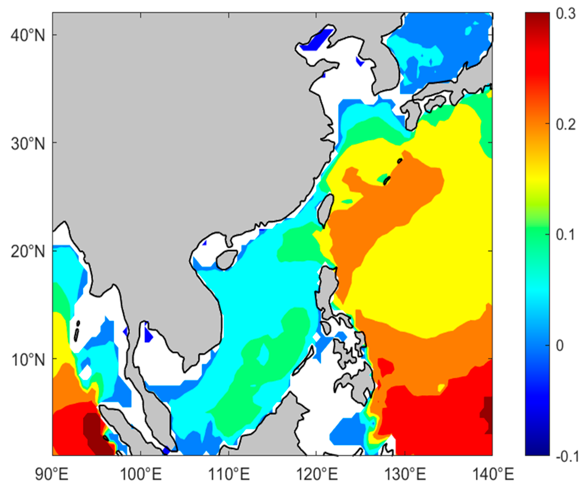
5.2. Regional Differences in EWHO

The present study analyzed regional variations in observed wave trends by calculating annual EWHO averages and averages for January–December for 1940–2022 at each grid point. Trends were identified through linear regression, and Figure 7 and Figure 8 show the regions in which these trends were shown to exceed 90% significance. Over half of the China seas exhibited clear annual increasing trends in EWHO (Figure 7), including Donghai and Nanhai (>0.10%/yr) and the waters east of the first island chain (>0.15%/yr, up to 0.30%/yr in the waters southeast of the Philippines). There were minimal areas with significant decreases in EWHO, concentrated around the Japanese Sea. No significant EWHO trends were observed in the Yellow Sea or Bohai Sea.

The present study identified a significant increasing trend in EWHO in the China seas from January to December, with notable regional variations in growth rates. There were significant increasing trends in EWHO throughout the year, exceeding 0.1%/yr in the regions east of the Ryukyu Islands, Taiwan Island, and the Philippine Islands. The most significant increase was in the waters southeast of the Philippines, reaching 0.50%/yr in April and May. There were increasing trends in EWHO in Donghai and Nanhai in January and April of 0.10–0.20%/yr, with no significant trends outside of this period. No significant EWHO trend was observed in the Yellow Sea or Bohai Sea from January to December.

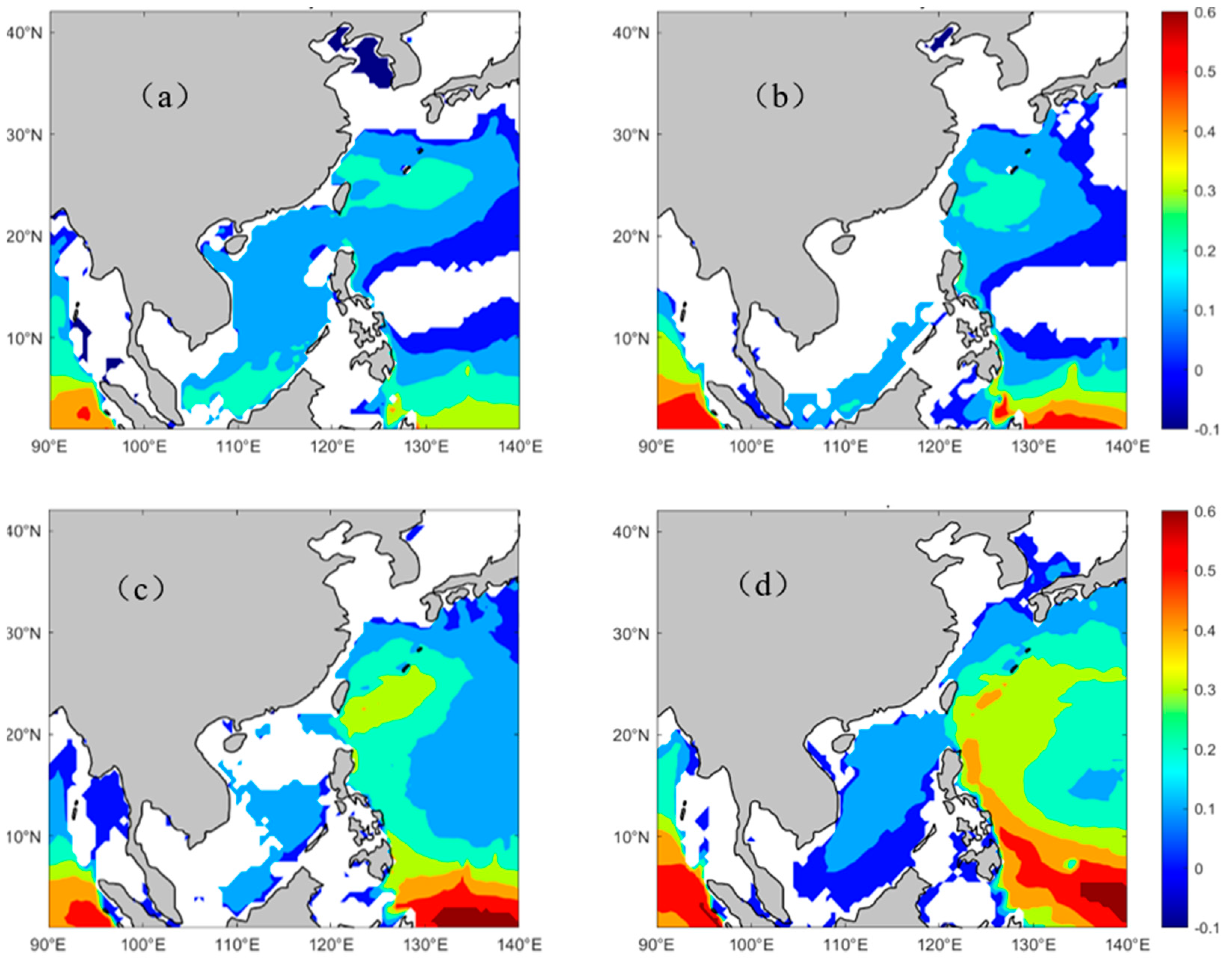
5.3. Dominant Month of EWHO Trends

The present study analyzed annual trends in EWHO (Figure 7) in conjunction with monthly trends (Figure 8) to identify the months over which the trends dominated across different regions. The results showed that April and December were the dominant months for trends in EWHO in the China seas, with the most significant increasing trend in April. Specifically, in Nanhai and Donghai, January and April were the months that dominated trends in EWHO; those for the southeastern waters of the Philippines were March to April and November to December; and those for the eastern sea of Taiwan Island were March to April and August to September. There was an overall significant correlation between EWHO spatial trends and EWHO values. For example, there were no apparent spatial trends in EWHO in regions with low EWHO, such as the Yellow Sea and Bohai Sea. There were relatively higher values of EWHO along the southeastern coast of the Philippines, with this region showing a significantly increasing trend.

6. Correlations Between EWHO and Climate Indices

6.1. Correlation Between EWHO and NINO3 Index

Due to the position of China on the western coast of the Pacific Ocean, an El Niño event results in changes to the distribution of wave heights in the China seas, in turn impacting the EWHO distribution. The present study analyzed the correlation between NINO3 and EWHO (Figure 9), identifying an overall significantly negative relationship. Higher correlations between NINO3 and EWHO were concentrated in Nanhai and the waters near the Philippines. Significant negative correlations between NINO3 and EWHO were observed from February to March and from June to August, with the highest correlation coefficient (<−0.40) in February. Conversely, there was a significant positive correlation between EWHO and NINO3 in the waters south of the Philippines from February to April, with correlation coefficients ranging from 0.30 to 0.50.

There were decreases and increases in atmospheric pressure in the Eastern Pacific and Western Pacific, respectively, during the positive phase of NINO3, corresponding to El Niño conditions, which contributed to a more stable atmospheric system. This stability weakened the winter monsoons over the China seas and significantly reduced wave height. With these decreases in wave height, there was a decrease in the frequency of waves within the available range, leading to a notable reduction in EWHO. Consequently, the EWHO in regions influenced by the winter monsoon exhibited a significant negative correlation with NINO3, particularly evident in February.

6.2. Correlation Between EWHO and AMOS

The coastal regions of China fall within a monsoon climate zone, with monsoons affecting both summer and winter conditions. The Australian Monsoon Index (AMOS) reflects the monsoon conditions over the Indian Ocean and the Western Pacific coast. The present study analyzed the correlation between the AMOS and the EWHO. As shown in Figure 10, there was a significant overall positive correlation between the AMOS and EWHO (see Figure 9), with particularly strong correlations in the waters southeast of the Philippines and east of Taiwan Island. Temporally, this significant positive correlation mainly manifested in January–April, September–October, and in December. A significant positive correlation between EWHO and the AMOS was observed from January to April and in December in the waters southeast of the Philippines, with the highest correlation in January at correlation coefficients of 0.40 to 0.50. There was a significant positive correlation between EWHO and the AMOS in the waters east of Taiwan Island from January to April and in September, with the strongest correlations in April and September at correlation coefficients of 0.30 to 0.40.

Changes in the AMOS were closely associated with the Australian monsoon, attributable to the influences of the monsoon on wind patterns and oceanic conditions across the Indo-Western Pacific region. Given the strong relationship between monsoon activity and the climate and ocean states of Nanhai and Donghai, variations in the AMOS indirectly affect wave heights in the China seas. Specifically, high AMOS levels from January to April result in the intensification of Western Pacific monsoon activity, thereby strengthening the Northeast Monsoon. This intensification results in increased swell and wind waves, leading to a notable rise in EWHO. Consequently, a significant positive correlation was established between EWHO and the AMOS, which was particularly pronounced during the monsoon season.

7. Suggestions for Site Selection for Wave Energy Development

This paper investigates the spatial–temporal distribution patterns and evolution of EWHO, which holds significant importance for wave energy development. The research findings indicate that the SWH and EWHO in the region bounded by Hainan Island, Taiwan Island, and Luzon Island are relatively high and consistently distributed throughout the year, facilitating a continuous supply of wave energy. Additionally, EWHO in this area exhibits a notable growth trend, positively influencing its future development. Moreover, EWHO in this region shows a significant correlation with the AMOS and NINO3, suggesting that changes in key climate indices can enhance the prediction of EWHO trends.

8. Conclusions

This study analyzed regional and temporal variations in EWHO in the China seas as well as the correlations between climate indices (NINO3, AMOS) and EWHO in the China seas and their underlying mechanisms. It is hoped that the results of this study can inform future long-term planning for wave energy development.

Higher-EWHO areas were concentrated in northern Nanhai (50~60%) and east of the first island chain (60~70%), whereas areas of lower EWHO were found in the Yellow Sea (10~20%), Bohai Sea (10~20%) and southern Nanhai (5~10%). Higher values of EWHO were found in January–February and November–December, whereas lower values were observed between May and July.

The EWHO and SWH showed notable spatial differences, with the latter in the sea area south of China exhibiting a significant north-to-south decreasing trend, whereas the former showed a relatively stable distribution without an obvious decreasing trend. Nanhai showed two major regions with higher EWHO: its northern part and the southeastern waters off the coast of Vietnam. In contrast, there was only one area with significantly higher SWH: the northern part of Nanhai.

There was an overall increasing temporal trend in EWHO in the China seas from 1941 to 2022 of 0.13%. There were significant regional differences in EWHO trends in the China seas. Areas with significant annual increases in EWHO were concentrated in the waters southeast of the Philippines (0.20–0.30%/yr) and east of Taiwan Island (0.20%/yr). Notable monthly variations were evident. The months with the most significant annual increases in EWHO were April (0.19%/yr) and December (0.11%/yr), with the highest growth rate southeast of the Philippines reaching 0.40–0.60%/yr in April.

NINO3 exhibited a significant negative correlation with EWHO in Nanhai and north of the Philippines, particularly from February to March and June to August, with February showing the most significant correlation (correlation coefficients ranging from −0.30 to −0.50). The correlation between EWHO and the AMOS in the southeastern waters of the Philippines was strongest in January, with correlation coefficients ranging from 0.40 to 0.50.

The AMOS exhibited a significant positive correlation with EWHO in the southeastern waters of the Philippines and the eastern waters of Taiwan Island, particularity from January to April and September to December. The correlation between EWHO and the AMOS in the eastern waters of Taiwan Island was most significant in April and September, with correlation coefficients ranging from 0.30 to 0.40.

References

1. Zheng, C.W.; Li, X.H.; Azorin-Molina, C.; Li, C.Y.; Wang, Q.; Xiao, Z.N.; Yang, S.B.; Chen, X.; Zhan, C. Global trends in oceanic wind speed, wind-sea, swell, and mixed wave heights. Appl. Energy 2022, 321, 119327. [Google Scholar] [CrossRef]
2. Wan, Y.; Zhang, J.; Meng, J.M.; Wang, J. Exploitable wave energy assessment based on ERA-Interim reanalysis data—A case study in the East China Sea and the South China Sea. Acta Oceanol. Sin. 2015, 34, 143–155. [Google Scholar] [CrossRef]
3. Wan, Y.; Zhang, J.; Meng, J.M.; Wang, J.; Dai, Y.S. Study on wave energy resource assessing method based on altimeter data—A case study in Northwest Pacific. Acta Oceanol. Sin. 2016, 35, 117–129. [Google Scholar] [CrossRef]
4. Iglesias, G.; Carballo, R. Choosing the site for the first wave farm in a region: A case study in the Galician Southwest. Energy 2011, 36, 5525–5531. [Google Scholar] [CrossRef]
5. Iglesias, G.; Carballo, R. Wave power for la isla bonita. Energy 2010, 3, 5013–5021. [Google Scholar] [CrossRef]
6. Khojasteh, D.; Mousavi, S.M.; Glamore, W.; Iglesias, G. Wave energy status in Asia. Ocean. Eng. 2018, 169, 344–358. [Google Scholar] [CrossRef]
7. Akpınar, A.; Bingolbali, B.; Van Vledder, G.P. Long-term analysis of wave power potential in the Black Sea, based on 31-year SWAN simulations. Ocean Eng. 2017, 130, 482–497. [Google Scholar] [CrossRef]
8. Shao, Z.X.; Liang, B.C.; Li, H.J.; Wu, G.X.; Wu, Z.H. Blended wind fields for wave modeling of tropical cyclones in the South China Sea and East China Sea. Appl. Ocean. Res. 2018, 71, 20–33. [Google Scholar] [CrossRef]
9. Semedo, A.; Suselj, K.; Rutgersson, A.; Sterl, A. A global view on the wind sea and swell climate and variability from ERA-40. J. Clim. 2011, 24, 61–79. [Google Scholar] [CrossRef]
10. Dodet, G.; Bertin, X.; Taborda, R. Wave climate variability in the North-East Atlantic Ocean over the last six decades. Ocean. Model. 2010, 31, 120–131. [Google Scholar] [CrossRef]
11. Gower, J.F.R. Temperature, wind and wave climatologies, and trends from marine meteorological buoys in the northeast Pacific. J. Clim. 2002, 15, 3709–3718. [Google Scholar] [CrossRef]
12. Sterl, A.; Caires, S. Climatology, variability and extrema of ocean waves: The web-based KNMI/ERA-40 wave atlas. Int. J. Climatol. 2005, 25, 963–978. [Google Scholar] [CrossRef]
13. Gulev, S.K.; Grigorieva, V. Variability of the winter wind waves and swell in the North Atlantic and North Pacific as revealed by the voluntary observing ship data. J. Clim. 2006, 19, 5667–5685. [Google Scholar] [CrossRef]
14. Gupta, N.; Bhaskaran, P.K.; Dash, M.K. Recent trends in wind-wave climate for the Indian Ocea. Curr. Sci. 2015, 108, 2191–2201. [Google Scholar]
15. Akpınar, A.; Jafali, H.; Rusu, E. Temporal variation of the wave energy flux in hotspot areas of the Black Sea. Sustainability 2019, 11, 562. [Google Scholar] [CrossRef]
16. Liang, B.C.; Liu, X.; Li, H.J.; Wu, Y.J.; Lee, D.Y. Wave Climate Hindcasts for the Bohai Sea, Yellow Sea, and East China Sea. J. Coast. Res. 2016, 32, 172–180. [Google Scholar]
17. Zheng, C.W.; Xiao, Z.N.; Peng, Y.H.; Li, C.Y.; Du, Z.B. Rezoning global offshore wind energy resources. Renew. Energy 2018, 129, 1–11. [Google Scholar] [CrossRef]
18. Wan, Y.; Zheng, C.; Li, L.; Dai, Y.; Esteban, M.D.; López-Gutiérrez, J.S.; Qu, X.; Zhang, X. Wave energy assessment related to wave energy convertors in the coastal waters of China. Energy 2020, 202, 117741. [Google Scholar] [CrossRef]
19. Falnes, J. A review of wave-energy extraction. Mar. Struct. 2007, 20, 185–201. [Google Scholar] [CrossRef]
20. Bertin, X.; Prouteau, E.; Letetrel, C. A significant increase in wave height in the NorthAtlantic Ocean over the 20th century. Glob. Planet Change 2013, 106, 77–83. [Google Scholar] [CrossRef]
21. Islek, F.; Yuksel, Y.; Sahin, C. Spatiotemporal long-term trends of extreme wind characteristics over the Black Se. Dyn. Atmos. Ocean. 2020, 90, 101132. [Google Scholar] [CrossRef]
22. Akpınar, A.; Bingölbali, B. Long-term variations of wind and wave conditions in the coastal regions of the Black Se. Nat. Hazards 2016, 84, 69–92. [Google Scholar] [CrossRef]
23. Başaran, B.; Güner, H.A.A. Effect of wave climate change on longshore sediment transport in Southwestern Black Sea. Estuar. Coast. Shelf Sci. 2021, 258, 107415. [Google Scholar] [CrossRef]
24. Zhang, X.; Zhang, J.; Fan, C.; Meng, J.; Wang, J.; Wan, Y. Analysis of Dynamic Characteristics of the 21st Century Maritime Silk Roa. J. Ocean. Univ. China 2018, 17, 487–497. [Google Scholar] [CrossRef]
25. Han, W.; Yang, J. Wave height possibility distribution characteristics of significant wave height in China Sea based on multi-satellite grid dat. Conf. Ser. Earth Environ. Sci. 2016, 46, 012033. [Google Scholar] [CrossRef]
26. Wang, Y.; Liu, Y.; Mao, X.; Chi, Y.; Jiang, W. Long-term variation of storm surge-associated waves in the Bohai Se. J. Oceanol. Limnol. 2019, 37, 1868–1878. [Google Scholar] [CrossRef]
27. Zheng, C.; Li, C. Overview of site selection difficulties for marine new energy power plant and suggestions: Wave energy case study. J. Harbin Eng. Univ. 2018, 39, 200–206. [Google Scholar]
Figure 1. Annual average significant wave height in China seas for 1940–2022 (a), unit: m. Computational area in map of China (b).
Jmse 13 01042 g001
Figure 2. Monthly average significant wave height from January to December (al) for 1940–2022, unit: m.
Jmse 13 01042 g002aJmse 13 01042 g002b
Figure 3. Annual distribution of effective wave height occurrence for 1940–2022, unit: %.
Jmse 13 01042 g003
Figure 4. Monthly distribution of effective wave height occurrence from January to December (al) for 1940–2022, unit: %.
Jmse 13 01042 g004aJmse 13 01042 g004b
Figure 5. Annual values (left) and monthly variation (right) in effective wave height occurrence for (a) 1940-2022, (b) 1940-1979, (c) 1980–2022; unit: %.
Jmse 13 01042 g005aJmse 13 01042 g005b
Figure 6. Effective wave height occurrence in each month (January–December) for 1940–2022(al), unit: %.
Jmse 13 01042 g006aJmse 13 01042 g006b
Figure 7. The annual trends in effective wave height occurrence for 1940–2022. Note: Only areas significant at the 0.1 significance level are shown; unit: %/yr.
Jmse 13 01042 g007
Figure 8. The monthly trends in effective wave height occurrence (EWHO) from January to December (al) for 1940–2022. Only areas significant at the 0.1 significance level are shown; unit: %/yr.
Jmse 13 01042 g008aJmse 13 01042 g008b
Figure 9. The correlation between effective wave height occurrence and NINO3 from January to December (al) for 1940–2022. Only areas significant at the 0.1 significance level are shown.
Jmse 13 01042 g009aJmse 13 01042 g009bJmse 13 01042 g009c
Figure 10. The correlation between effective wave height occurrence and the Australian Monsoon Index (AMOS) from January to December (al) for 1940–2022. Only areas significant at the 0.1 significance level are shown.
Jmse 13 01042 g010aJmse 13 01042 g010bJmse 13 01042 g010c
Disclaimer/Publisher’s Note: The statements, opinions and data contained in all publications are solely those of the individual author(s) and contributor(s) and not of MDPI and/or the editor(s). MDPI and/or the editor(s) disclaim responsibility for any injury to people or property resulting from any ideas, methods, instructions or products referred to in the content.