Article

LatentResNet: An Optimized Underwater Fish Classification Model with a Low Computational Cost

1
Electrical and Electronics Engineering Department, Çukurova University, 01330 Adana, Turkey
2
Section for Fisheries Technology, National Institute of Aquatic Resources (DTU Aqua), Technical University of Denmark, 9850 Hirtshals, Denmark
3
Biomedical Engineering Department, Çukurova University, 01330 Adana, Turkey
*
Author to whom correspondence should be addressed.
J. Mar. Sci. Eng. 2025, 13(6), 1019; https://doi.org/10.3390/jmse13061019
Submission received: 14 April 2025 / Revised: 19 May 2025 / Accepted: 21 May 2025 / Published: 23 May 2025
(This article belongs to the Section Ocean Engineering)

Abstract

:
Efficient deep learning models are crucial in resource-constrained environments, especially for marine image classification in underwater monitoring and biodiversity assessment. This paper presents LatentResNet, a computationally lightweight deep learning model involving two key innovations: (i) using the encoder from the proposed LiteAE, a lightweight autoencoder for image reconstruction, as input to the model to reduce the spatial dimension of the data and (ii) integrating a DeepResNet architecture with lightweight feature extraction components to refine encoder-extracted features. LiteAE demonstrated high-quality image reconstruction within a single training epoch. LatentResNet variants (large, medium, and small) are evaluated on ImageNet-1K to assess their efficiency against state-of-the-art models and on Fish4Knowledge for domain-specific performance. On ImageNet-1K, the large variant achieves 66.3% top-1 accuracy (1.7M parameters, 0.2 GFLOPs). The medium and small variants reach 60.8% (1M, 0.1 GFLOPs) and 54.8% (0.7M, 0.06 GFLOPs), respectively. After fine-tuning on Fish4Knowledge, the large, medium, and small variants achieve 99.7%, 99.8%, and 99.7%, respectively, outperforming the classification metrics of benchmark models trained on the same dataset, with up to 97.4% and 92.8% reductions in parameters and FLOPs, respectively. The results demonstrate LatentResNet’s effectiveness as a lightweight solution for real-world marine applications, offering accurate and lightweight underwater vision.

1. Introduction

Neural networks have demonstrated exceptional capabilities in computer vision tasks, such as image classification [1,2,3], object detection [4,5,6], and segmentation [7,8,9]. These advancements have enabled the analysis of large-scale visual data, driving technological progress across multiple domains, including marine science and underwater exploration. For example, deep neural networks have played a critical role in marine biodiversity monitoring [10], automated fish species identification [11], habitat mapping [12], and pollution assessment [13] using underwater imagery.
However, the computational demands of deep neural networks pose significant challenges, particularly in marine research, where real-time processing is often required in remote, resource-constrained environments. Deploying these models on autonomous underwater vehicles (AUVs), remotely operated vehicles (ROVs), and underwater devices is especially difficult due to limited processing power, memory, and battery life. For example, marine researchers conducting real-time marine species analysis in underwater environments rely on low-power embedded devices equipped with Nvidia Jetson Xavier, Santa Clara, CA, USA to classify species on-site, reducing the need for large-scale data transmission [14]. Alternatively, the usage of Nvidia AGX Orin can be helpful in achieving near real-time processing speed for detecting and tracking Nephrops in underwater videos [15]. Similarly, underwater surveillance systems monitoring coral reef health require efficient algorithms to process vast image datasets without overloading onboard hardware [16]. These constraints highlight the critical need for lightweight, energy-efficient deep learning models that can perform high-accuracy image classification and object detection without excessive computational load.
To address this challenge, researchers have explored various strategies, including the usage of low computation operations, including bottleneck layers [17] and depthwise separable convolutions [18], that are incorporated into deep neural networks. Additionally, architectural enhancements, such as replacing the traditional full convolutional process in Convolutional Neural Networks (CNNs) with group convolutions [19], can make the process more computationally efficient. Other methods such as NAS (Neural Architecture Search) [20] are also used to design efficient neural network architectures that achieve high performance with minimal computational cost.
This study builds upon these efforts by proposing a novel lightweight deep learning model, namely LatentResNet, designed for underwater image classification, balancing high accuracy with reduced computational complexity to support real-time underwater monitoring for marine applications. The proposed model has an encoder as the initial step, which is followed by a series of modified ResNet blocks, namely DeepResNet blocks (DRBs). The encoder is trained as a separate procedure using an efficient autoencoder architecture called LiteAE for image reconstruction. Therefore, this step compresses the spatial dimensions and extracts the most relevant features. DRBs further process the features extracted by the encoder block through their improved depth components.
The experimental results proved that using the encoder, which was trained for image reconstruction task, as an input to the classification model provides useful features for the classification process. This approach reduces spatial dimensions and, consequently, the computational cost of subsequent processes. On the other hand, DRBs were able to efficiently process these features, resulting in strong classification performance with reduced computational complexity.
The major contributions of this study can be listed as follows:
  • Proposing a lightweight autoencoder named LiteAE and lightweight feature extraction and refining blocks called DeepResNet blocks, inspired by the well-known ResNet block: the computational cost of DeepResNet blocks is lower than ResNet blocks, and their presence in the model architecture improves the underwater image classification accuracy.
  • Efficiency of using the encoder part of LiteAE model as a suitable tool for extracting discriminative features from underwater imagery while compressing the input data: this approach leads to classification models with lower computational costs while reducing the computational load, making it more suitable for marine applications in remote applications.
  • Proposing the LatentResNet model, which integrates the encoder part of LiteAE with DeepResNet blocks for underwater image classification: LatentResNet is available in three scaled versions: small, medium, and large, achieved by modifying the number of DeepResNet blocks or number of units inside DeepResNet blocks; these variations are designed to accommodate a range of devices with different computational capacities. The source code has also been made available at https://github.com/MuhabHariri/LatentResNet (accessed on 20 May 2025)
The remainder of this paper is organized as follows: In Section 2, the existing studies in the related field are reviewed. In Section 3, the proposed methods, model, and training strategy are discussed. Section 4 represents the results and discussion. Finally, the paper is concluded in Section 5.

2. Related Work

Research in the field of resource-constrained machine learning is gaining significant attention from researchers. In general, the primary focus of researchers is to achieve optimal performance while minimizing computational costs [21].
Techniques aimed at reducing the computational cost of classification and object detection models, including the development of low-cost models, generally fall under two categories: Low-Complexity Model Construction and Neural Network Compression. Low-Complexity Model Construction focuses on designing models from scratch with efficiency as a primary goal, while Neural Network Compression involves reducing the size and computational demands of existing models.
The MobileNet series [22,23,24] is categorized under Low-Complexity Model Construction, where the authors used lightweight techniques like depthwise separable convolutions, inverted residual blocks, and Squeeze-and-Excitation (SE) modules to produce efficient models. The EfficientNet series [25] employed NAS and proposed the Compound Model Scaling method, along with similar techniques used in the MobileNet series, to create models with low computational cost. The use of Low-Complexity Model Construction strategies has been extensive, resulting in many lightweight models in the classification domain. For instance, Han et al. [26] proposed the Ghost Module to generate more feature maps from inexpensive operations, leading to GhostNet model variants with a low number of floating point operations per second (FLOPs). Overall, many lightweight models, such as RegNet [27], EdgeNeXt [28], and MobileVIT [29], have been produced using the Low-Complexity Model Construction approach.
The domain of Neural Network Compression includes techniques such as pruning [30,31,32], low-bit quantization [33,34,35], and knowledge distillation [36,37,38]. These techniques focus on eliminating dispensable parts of existing models, reducing the bit precision in neural network calculations, and training smaller models to mimic larger ones, respectively. These methods rely on carefully balancing the trade-off between sacrificing a small amount of accuracy for significantly more computationally efficient models.
Scaling the model is an optimization technique used in machine learning to adapt a model’s architecture to varying computational resources and performance requirements. This is done by adjusting the model’s depth (number of layers), width (number of channels), and input resolution. While scaling can be considered during the initial model design, it is often used as a flexible tool after the base model is designed. Typically, scaling is applied after the Low-Complexity Model Construction or Neural Network Compression techniques to further optimize the model for specific needs. This method enables the customized production of models that achieve a balance between computational efficiency and desired performance. Wu et al. [39] used Differentiable Neural Architecture Search (DNAS) to scale models by optimizing layer choices, input resolution, and channel sizes. The paper proposed device-specific models, like FBNet-S8 and FBNet-iPhoneX, tailored for different smartphones to balance accuracy, latency, and efficiency. Tan and Le [40] introduced EfficientNetV2, a model that incorporates a scaling method to optimize depth, width, and resolution, with a focus on achieving smaller model sizes and faster training times. By combining training-aware NAS with refined compound scaling, EfficientNetV2 produces models such as EfficientNetV2-S, EfficientNetV2-M, and EfficientNetV2-L, which balance accuracy, efficiency, and speed. Howard et al. [24] discussed the use of model scaling as part of their MobileNetV3 architecture optimization process. They employed techniques such as adjusting the number of filters per layer to optimize the model’s architecture. Additionally, they used different multipliers for depth, width, and input resolution to effectively scale the model for varying computational resources and performance requirements. This kind of scaling is used to balance the trade-off between accuracy and efficiency, particularly targeting mobile devices with varying capabilities.
The application of autoencoders to reduce the dimensionality of input data, followed by leveraging the resulting lower-dimensional representations as inputs for classification models, has been used by other researchers in earlier studies. For instance, Sharma et al. [41] employed a convolutional autoencoder-based architecture with a Class-Specific Self-Expressiveness (CSSE) layer to compress input data and generate features from the Extended Yale B Face, MNIST, and COIL-20 datasets. These representations were subsequently used with classifiers, specifically k-Nearest Neighbors (k-NN) and Sparse Representation (SR) for classification. Similarly, Gogna et al. [42] utilized a stacked discriminative autoencoder (DiAE) with fully connected layers, where the output from the final layer of the stacked encoder was passed to classifiers such as k-NN, a Support Vector Machine (SVM), and Sparse Representation Classifier (SRC) for classification. The model was evaluated on multiple datasets, including MNIST and its variants and USPS datasets. Kong et al. [43] trained an autoencoder consisting of CNN layers, where the encoder compresses seismic time-series data into a lower-dimensional representation. The features extracted by the encoder are then passed through optional additional CNN layers followed by a fully connected layer. All these works demonstrated the effectiveness of the encoder in compressing data and extracting the features required for classification. However, the application of convolutional layer-based encoders to complex classification tasks, particularly on challenging datasets like ImageNet-1K and Fish4Knowledge, has not been thoroughly investigated to assess their effectiveness. In this work, the proposed LatentResNet model is first evaluated on the ImageNet-1K dataset, which is commonly used as a benchmark for classification tasks, and then fine-tuned on the Fish4Knowledge dataset for fish species recognition. Evaluating the model on the ImageNet-1K dataset provides an opportunity to assess its performance, particularly its efficiency, in comparison with other common benchmark models under standardized conditions. Additionally, the rich set of features extracted during pretraining on ImageNet are intended to be utilized, as they are known to generalize well across a wide range of visual tasks. These features serve as a strong foundation for downstream applications, particularly in domain-specific scenarios such as marine species classification.

3. Materials and Methods

The LatentResNet model consists of two major components: (i) the encoder part of an autoencoder to reduce the spatial dimensions of the model input and (ii) DeepResNet blocks (DSBs) to refine and enhance the feature extraction process. The following subsections first introduce the Fish4Knowledge dataset, on which the LatentResNet is fine-tuned, then describe the two main components, and finally present the overall architecture and training strategy of the proposed model.

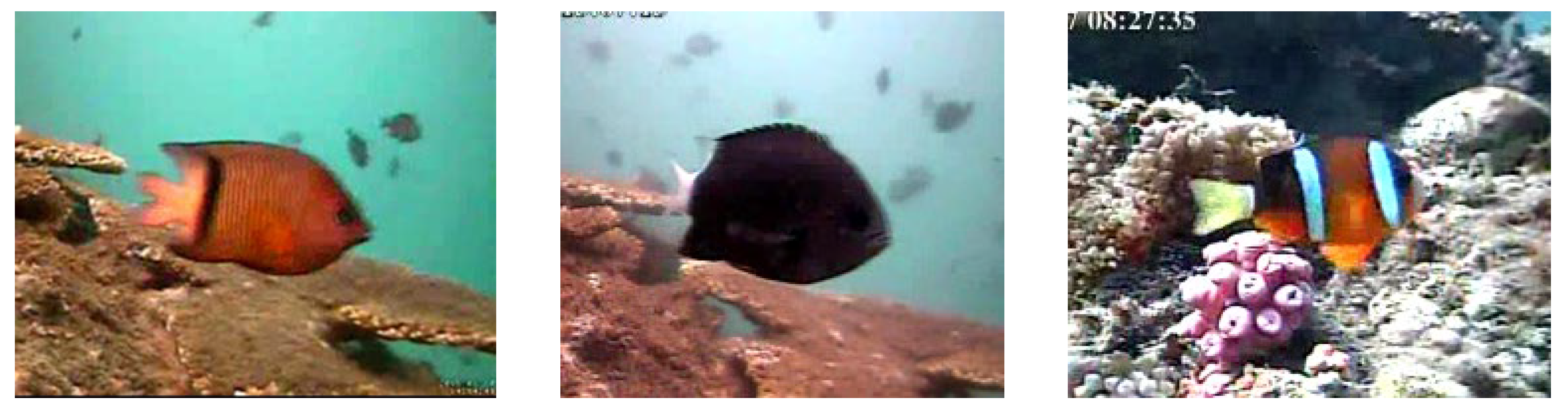
3.1. Fish4Knowledge Dataset

The Fish4Knowledge dataset [44] is a publicly available benchmark dataset designed for fish species classification in underwater environments. It contains 27,370 labeled images across 23 different fish species. The dataset includes images of varying resolutions and is a curated subset of the larger Fish4Knowledge project, which processed over 90,000 h of underwater video and tracked more than 1 billion fish. The data were gathered by the Taiwan Power Company, Taiwan Institute of Oceanography, and Kenting National Park during the period from 1 October 2010 to 30 September 2013. In this study, 20% of the images from each class were used as the test set. Figure 1 shows samples from the Fish4Knowledge dataset.

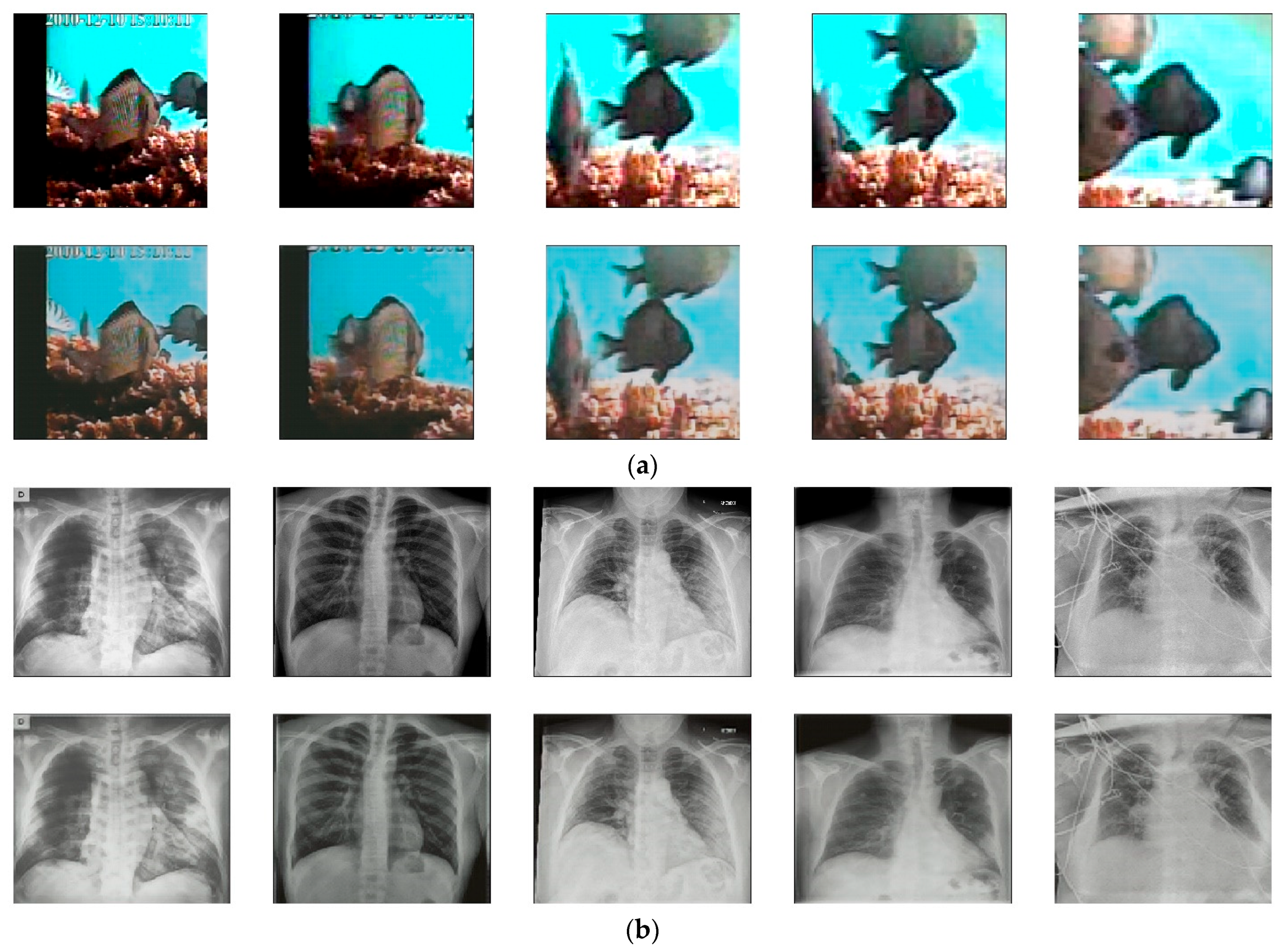
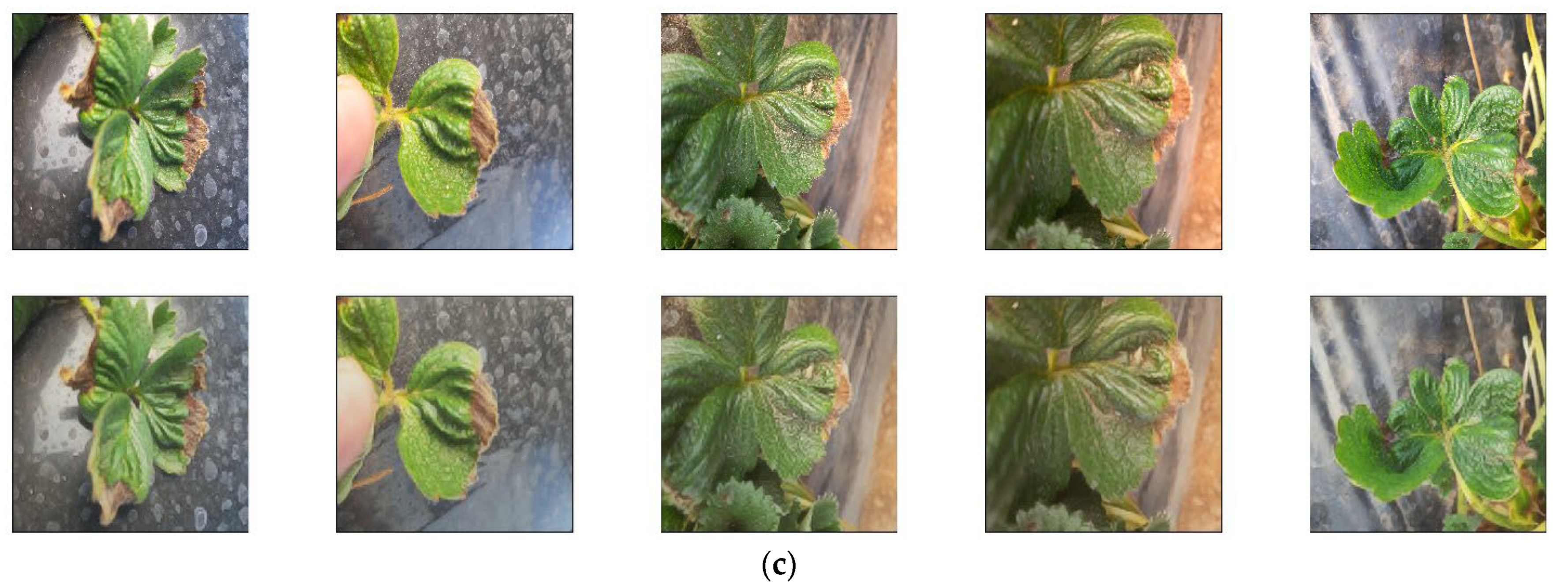
3.2. Autoencoder Design

The autoencoder is a type of neural network architecture commonly used for unsupervised learning tasks [45]. The autoencoder comprises two main components: the encoder and the decoder. The encoder compresses the input data into a lower-dimensional representation, often referred to as the “latent space” or “code”, capturing important features of the input data. The decoder then reconstructs the original input data from this compressed representation. The autoencoder network is trained to minimize the difference between the original input and the reconstructed output. This process enables learning a compact and informative representation of the input data, which may be used as a dimensionality reduction tool.
The proposed network for image reconstruction is LiteAE, a lightweight and symmetric autoencoder designed for efficient performance (Figure 2). LiteAE is composed of three processing blocks in the encoder and three corresponding blocks in the decoder. Each processing block in the encoder consists of depthwise separable convolutional layer, batch normalization (BN), LeakyReLU activation functions, spatial dropout layers, and Efficient Channel Attention (ECA) layers. The spatial dropout [46] and ECA [47] layers are specifically included to enhance the robustness and feature selection capabilities of the model, respectively. In the decoder, the depthwise separable convolutional layers are replaced by transposed convolutional layers to facilitate upsampling and accurate reconstruction of the input data. Table 1 presents the metrics related to computational cost of the autoencoder LiteAE, such as the number of parameters and FLOPs associated with the encoder and decoder parts, respectively.

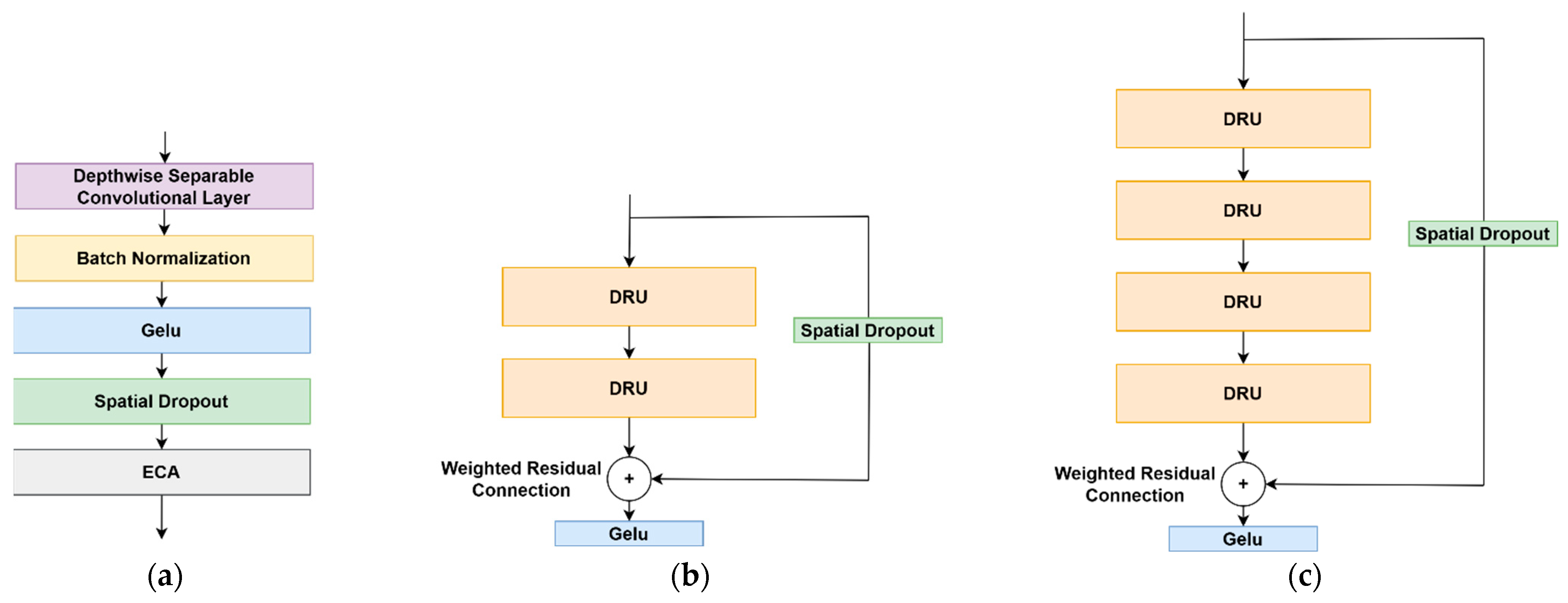
3.3. DeepResNet Block (DRB) Architecture

To further process the features generated by the encoder, a novel DeepResNet block (DRB) architecture, inspired by the well-known ResNet block, is proposed. The DRB consists of a series of cascaded DeepResNet Units (DRUs) in the transformation path, along with a spatial dropout layer incorporated into the residual path to enhance regularization. Two types of DRBs are introduced: DRB-2 (Figure 3b), which consists of two DRUs, and DRB-4 (Figure 3c), which consists of four DRUs. This design allows for flexibility in network depth and capacity.
In both DRB types, the input to the first DRU or the DRB itself is initially processed through the spatial dropout layer. This input also flows in parallel through the DRUs sequence. The outputs from both paths, the spatial dropout and the last DRU, are then combined by a weighted residual connection [48]. Finally, the resulting feature representation is passed through a GELU activation function to produce the final DRB output (Figure 3b,c).
Each DRU employs a depthwise separable convolution layer, which replace the traditional convolutional layers used in the original ResNet block [17]. Depthwise separable convolutions decompose the standard convolution operation into two separate processes: depthwise convolution and pointwise convolution. In the depthwise convolution, a single convolutional filter is applied to each input channel independently. The pointwise convolution then applies a 1 × 1 convolution to combine the output of the depthwise convolutions. This decomposition significantly reduces the number of parameters and computational complexity compared to standard convolutions, which simultaneously convolve across both spatial dimensions and depth channels. As a result, depthwise separable convolutions enhance the efficiency of DRUs, allowing for deeper architectures with lower computational costs. This separable layer in DRUs is followed by batch normalization and the GELU [49] activation function, which is used in place of ReLU as found in the native ResNet block. The final layer of the DRUs is the Efficient Channel Attention (ECA) mechanism, which improves model performance by emphasizing important channels. ECA is a lightweight attention mechanism designed to enhance feature representation in deep learning models by selectively emphasizing important channels without introducing high computational costs. Unlike traditional attention mechanisms, ECA avoids dimensionality reduction and instead applies a simple 1D convolution to capture cross-channel interactions, leading to efficient yet effective feature refinement.
Initial experiments revealed that the combination of layers in the DRU (Figure 3a), including the depthwise separable layer, batch normalization, GELU, and ECA, was highly prone to overfitting. Various regularization techniques, such as more aggressive data augmentation and L2 regularization, were tested but proved ineffective in mitigating the overfitting issue. However, spatial dropout emerged as the most effective method for reducing overfitting in the proposed block. Therefore, spatial dropout is added after each GELU activation function within each DRU.
Unlike standard dropout, which randomly drops individual neurons, spatial dropout discards entire feature maps (channels) during training. The demonstrated effectiveness of spatial dropout in reducing overfitting suggests that the encoder portion of the proposed classification model, or the DRB itself, produces feature maps with high correlation, contributing to overfitting. By randomly dropping a portion of entire feature maps during training, spatial dropout discourages the network from over-relying on specific channels and promoting more robust and distributed feature representations. This, in turn, enhances the robustness and generalization ability of the model
The standard residual connection found in the traditional ResNet block is replaced by a weighted residual connection in the DRB. The weighted residual connection introduces an adaptive mechanism, granting the network greater control over the influence of the residual connection on the output. This process is carried out by a trainable weight applied to the residual before it is added to the input. This allows the network to dynamically modulate the influence of the residual during training, effectively diminishing its impact when the weight is close to zero or amplifying it when the weight is larger. Equation (1) describes the process of the weighted residual connection.
Y = X + W   ·   R
In Equation (1), the output Y is calculated by adding the input X to a weighted version of the residual R, where the weight W is a trainable parameter that determines how much the residual should influence the final output. The same mechanism is illustrated in Listing 1 for implementation clarity.
Listing 1. Weighted residual connection in DRB.
Input:  X
Residual path:  R  = F( X )
Trainable scalar:  W  #Learned during training
Output:  Y  =  X  +  W  ·  R
Listing 1 illustrates the step-by-step implementation of the weighted residual connection in the DRB. The process begins with the input X , which represents the original feature representation entering the block. Simultaneously, X is processed through a transformation function, represented as F( X ), to produce the residual path output R . The transformation function F( X ) corresponds to the sequential operations performed within the DeepResNet Units (DRUs). This residual path captures additional learned features that contribute to the final representation. Unlike the standard ResNet block, where the residual is added directly to the input, the DRB employs a weighted residual connection, which introduces a trainable scalar parameter W that adjusts the impact of the residual before it is combined with X . This weight is learned during training, allowing the network to control the extent to which the residual influences the final output. If W is close to zero, the contribution of the residual path is minimized, while larger values of W increase its influence. The final output Y is computed by adding the weighted residual W · R to the original input X , as represented in the listing.

3.4. The LatentResNet Model

The base architecture of LatentResNet model involves an encoder as the initial step, and it is followed by sequences of DRBs (Figure 4). The encoder component of the autoencoder, as detailed in Section 3.2. and illustrated in Figure 2, is isolated after the complete autoencoder has been trained on the ImageNet-1K dataset. This isolated encoder is then employed as input to the DRBs in the subsequent parts. However, the spatial dropout layers within the encoder are removed, while the weights of the remaining layers are preserved.
To have flexibility in the model design and experiment with different model complexities, three versions of LatentResNet are defined: large, medium, and small, referred to as LatentResNet-L, LatentResNet-M, and LatentResNet-S, respectively. In LatentResNet-L (Figure 4), the output of the encoder is processed through three hierarchical sequences of DRB-4 (Figure 3c), with each sequence consisting of two DRB-4. Between each sequence, a max-pooling layer is introduced to reduce the spatial dimensions progressively. The output from the last DRB-4 sequence is passed through a global average pooling layer to reduce spatial dimensions and generate a compact feature vector. The output is then passed through classic dropout layer, followed by a batch normalization layer, and finally flattened. The model ends with either 23 or 1000 units representing the number of classes in the Fish4Knowledge or ImageNet-1K dataset, respectively.
Medium and small versions are derived through a systematic reduction in the complexity of the LatentResNet-L model. LatentResNet-M is obtained by removing one DRB-4 from each pair of DRB-4. On the other hand, LatentResNet-S is obtained by replacing each pair of the three hierarchical sequences of DRB-4 in LatentResNet-L with a single DRB-2.

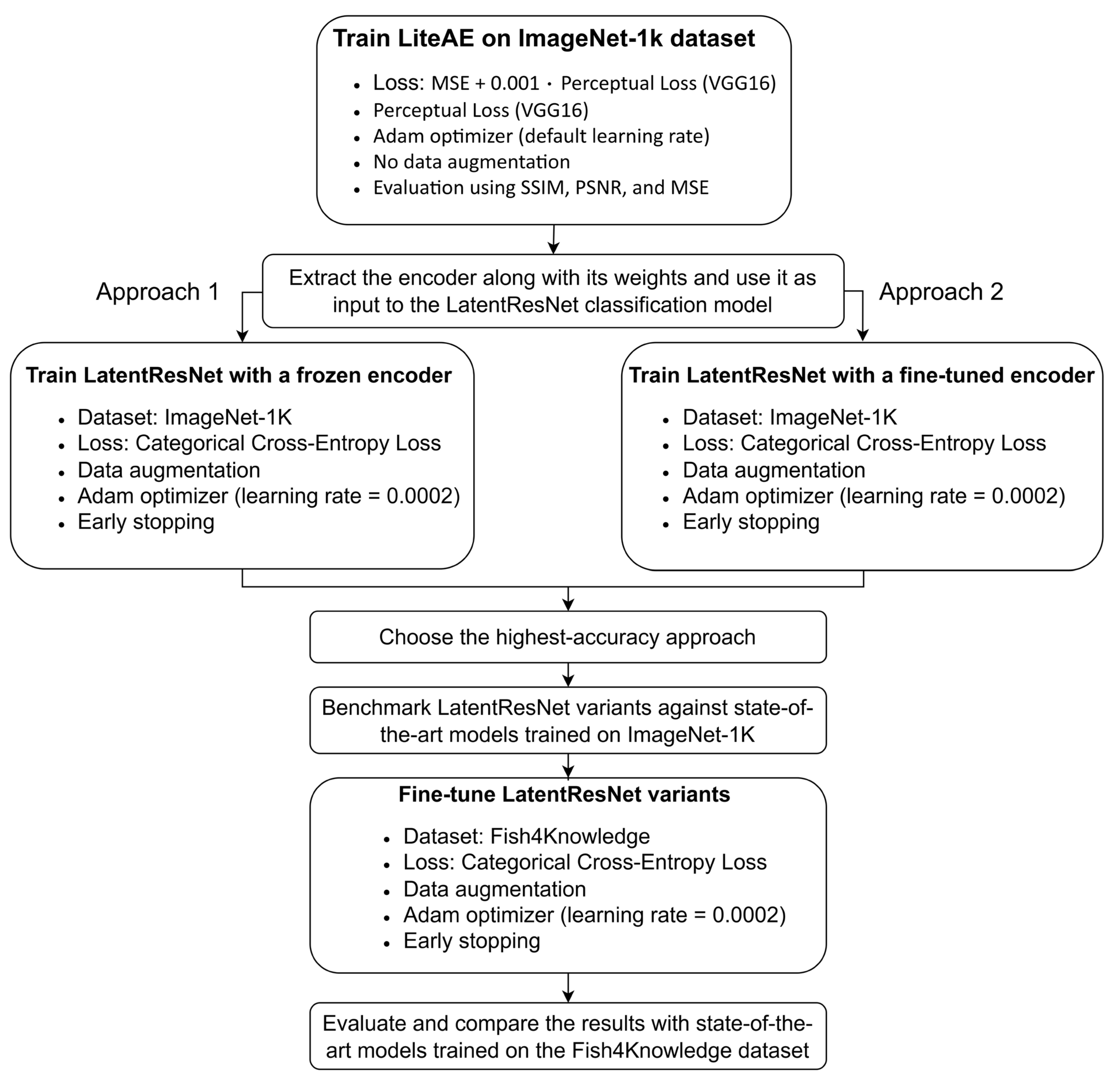
3.5. Training Strategy and Implementation Details

Although the encoder part of the autoencoder will eventually be used for fine-tuning LatentResNet on a fish-specific dataset (i.e., Fish4Knowledge), the ImageNet-1K dataset was chosen to train the autoencoder. This decision was based on the fact that ImageNet-1K includes a much higher number of images and classes, including many fish classes, making it a more comprehensive choice. Additionally, the LatentResNet model will be evaluated on the ImageNet-1K dataset to assess its efficiency and performance against state-of-the-art benchmark models such as MobileNetV3 and GhostNet.
The loss function used in training the LiteAE model is the sum of the mean squared error loss (MSE) and a perceptual loss from a pretrained VGG16 model. The MSE compares the true and reconstructed images at the pixel level, while the perceptual loss compares their high-level feature representations by passing them through the intermediate layer of VGG16 model. The perceptual loss helps the model in extracting finer, more meaningful visual features. The perceptual loss is scaled by 0.001 to provide subtle perceptual guidance, promoting both pixel accuracy (from MSE) and perceptual quality at the output of the autoencoder. The formulation is presented in Equations (2)–(4), which define the overall loss function of the LiteAE autoencoder L A E , the MSE loss L M S E , and the perceptual loss L P e r c , respectively.
L A E = L M S E + 0.001   L P e r c
L M S E = 1 N i = 1 N x i x ^ i 2 2
L P e r c = 1 N i = 1 N ϕ l ( x i ) ϕ l ( x ^ i ) 2 2 C l × H l × W l
Here, x i and x ^ i represent the original and reconstructed images for the ith sample, respectively. The batch size is denoted by N . The function ϕ l ( ) refers to the activation output from layer l of a frozen VGG-16 network, where the spatial dimensions of the feature map are given by H l × W l and the number of channels is C l .
The Adam optimizer was used for training LiteAE with its default parameters, and no data augmentation was applied to the training data images to preserve the original data structure, ensuring accurate reconstruction where the direct mapping from input to output is prioritized. To evaluate the performance of the autoencoder, several image reconstruction evaluation metrics were calculated, including the MSE, Peak Signal-to-Noise Ratio (PSNR), and Structural Similarity Index (SSIM) [50]. The MSE is calculated by averaging the squared differences between the original and reconstructed pixel values. The PSNR is computed as the logarithmic ratio between the maximum possible signal value and the noise power introduced by the reconstruction error, where a higher PSNR indicating better reconstruction quality. The SSIM, proposed to address some limitations of the MSE and PSNR, measures the similarity between two images by comparing local patterns of pixel intensities in terms of luminance, contrast, and structure. The formulations for PSNR and SSIM are provided in Equations (5) and (6), respectively.
P S N R ( x , x ^ ) = 10 log 10 ( M A X I 2 L M S E )
S S I M x , x ^ = ( 2 μ x μ x ^ + C 1 ) ( 2 σ x x ^ + C 2 ) ( μ x 2 + μ x ^ 2 + C 1 ) ( σ x 2 + σ x ^ 2 + C 2 )
M A X I denotes the highest possible intensity and is set to 255 for 8-bit RGB images. The constants C 1   = (0.01 × M A X I )2 and C2 = (0.03 × M A X I )2 are stability constants used in the SSIM formula to prevent division by zero or numerical instability. The term μ x represents the local mean of the original image, and σ x 2   denotes its local variance.
Subsequently, the trained encoder was separated and integrated as the input to the sequences of DRBs, as shown in Figure 4. The training strategy for the LatentResNet model comprises two approaches. In the first approach, the weights extracted by the encoder, initially trained for image reconstruction, are frozen, while the rest of the LatentResNet model is trained. In the second approach, the encoder’s weights are not frozen and fine-tuned during the training process. The first approach evaluates the effectiveness of the features learned by the encoder during image reconstruction for the classification task. On the other hand, the second approach examines whether fine-tuning the encoder, initially trained on image reconstruction, can further enhance the model performance. After training the LatentResNet model on the ImageNet-1K dataset, the model is fine-tuned on the Fish4Knowledge dataset. The steps of the entire training and evaluation pipeline are shown in Figure 5 to support a clear explanation of the procedure. For both training the model on ImageNet-1K and fine-tuning on Fish4Knowledge dataset, data augmentation techniques (Table 2) were applied on the training data. This included random shear, translation, zoom, rotation, horizontal flipping, and adjustments to the brightness, contrast, saturation, and color channels. The Adam optimizer was used for training with its default parameters, except for the learning rate, which was set to 0.0002. A batch size of 32 was chosen, and early stopping was implemented with a patience of 15 epochs, based on validation accuracy. Additional architectural hyperparameters, including the number of filters, spatial dropout, and classic dropout rates used in each model variant, are summarized in Table 3.
All the experiments were carried out on a high-performance computing system of Technical University of Denmark [51], particularly utilizing Tesla A100-PCIE GPUs. The codes were written in Python 3.10, and TensorFlow 2.10.2 was used to design the models.

4. Results and Discussion

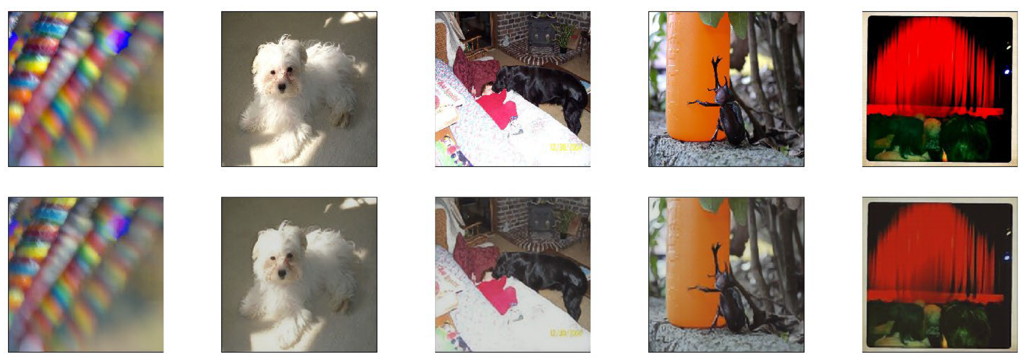
4.1. Experiments on Autoencoder (LiteAE)

The autoencoder LiteAE was trained using the ImageNet-1K dataset for a single epoch. The experiments showed that extending the training to additional epochs leads to overfitting, as evidenced by an increase in validation loss coupled with a decrease in training loss. The test subset of the ImageNet-1K dataset was employed to assess the performance of the autoencoder. The autoencoder LiteAE achieved a training loss of 0.0193 and a validation loss of 0.0110, demonstrating low reconstruction error and effective generalization during inference. Figure 6 presents both the input and the reconstructed images using the test samples of ImageNet-1K dataset.
Visual inspection reveals that the autoencoder was able to preserve the general structure and high-level features of the original images. As seen in the reconstructions of the original images in Figure 6, the primary objects remain identifiable, and key elements such as shapes and basic textures are preserved. However, the model consistently struggles with finer details, resulting in a slight blurring effect across all reconstructed images.
For further evaluation of the robustness of LiteAE on diverse problems, three datasets that are dedicated for specific problems were utilized. These datasets include underwater images for fish species recognition (Fish4Knowledge), X-ray images for medical diagnosis [52], and strawberry leaves for disorder detection [53]. The LiteAE model, with the same weights obtained from training on the ImageNet-1K dataset, was used to reconstruct images from these datasets (Figure 7). The results show that while the autoencoder retained the basic structure of the input data, it struggled with intricate details, a similar situation with the ImageNet-1K dataset. Fish images (Figure 7a) were well reconstructed in terms of overall structure, but finer details like edges and textures were partially lost, leading to slightly blurred outputs. The X-ray reconstructions show the overall anatomy but lack the clarity required for medical assessment (Figure 7b). Similarly, in the strawberry leaf images, the autoencoder captured the general structure but missed the finer texture and vein patterns, which might be crucial for tasks like disease detection (Figure 7c). These observations show that while the autoencoder LiteAE can generalize well across different types of datasets, its usage may not be suitable for tasks requiring highly detailed reconstructions, such as those involving medical imaging or fine texture analysis. In such cases, fine-tuning on the new dataset may be required to improve reconstruction quality and better capture intricate details.
In addition to the qualitative analysis through visual inspection, the performance of LiteAE was evaluated quantitatively by calculating the metrics mentioned in Section 3.5 on all the four datasets mentioned earlier (Table 4). According to the quantitative results on the ImageNet-1K test set, the SSIM score of 0.7508 suggests a moderate to good preservation of structural details, contrast, and luminance. The PSNR of 23.15 dB reflects a moderate level of image reconstruction quality. Finally, the MSE of 0.0067 signifies a low average squared error between the reconstructed and original images, confirming relatively low distortion in pixel intensities.
The LiteAE autoencoder achieved the highest SSIM (0.8436) on Fish4Knowledge dataset, indicating superior structural similarity and overall image quality. Achieving a better SSIM on the Fish4Knowledge dataset compared to ImageNet-1K, which the model was trained on, can be attributed to the lower visual complexity of Fish4Knowledge compared to ImageNet-1K. On the other hand, the strawberry dataset exhibits the highest PSNR (23.40 dB), meaning that the reconstructed image is most similar to the original in terms of pixel-level accuracy. The lower MSE (0.0049) for the X-ray dataset, despite its lower SSIM and PSNR compared to the ImageNet-1K, Fish4Knowledge and strawberry leaf datasets, can be attributed to the inherent characteristics of X-ray images. These images typically feature high contrast and minimal pixel intensity variability, which facilitates more accurate error minimization by the autoencoder compared to the other datasets.
These results demonstrate that the LiteAE autoencoder achieved high performance in reconstructing images and generalizing across various types of datasets. This suggests that the encoder was effective in capturing the most relevant features. However, the reconstructed images showed lower performance in capturing finer and intricate details, indicating that the encoder struggled to capture these more complex features.

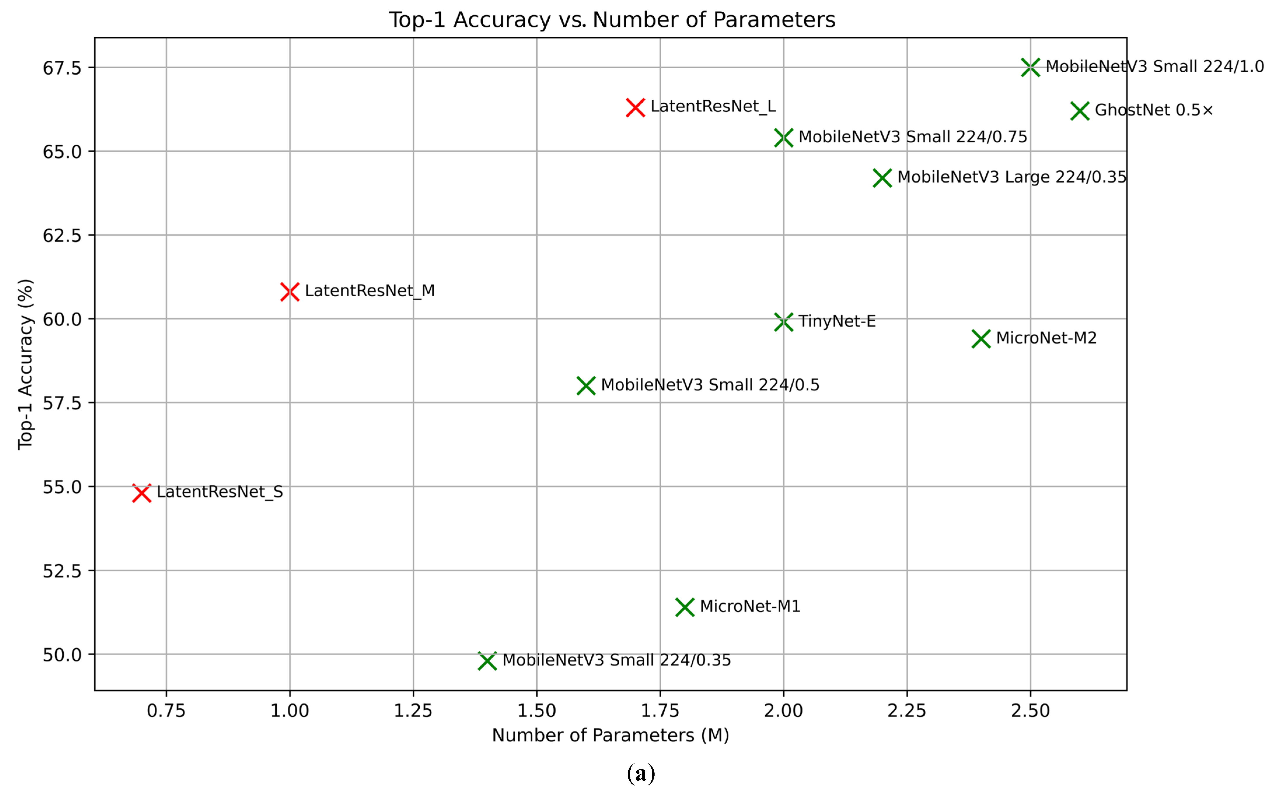
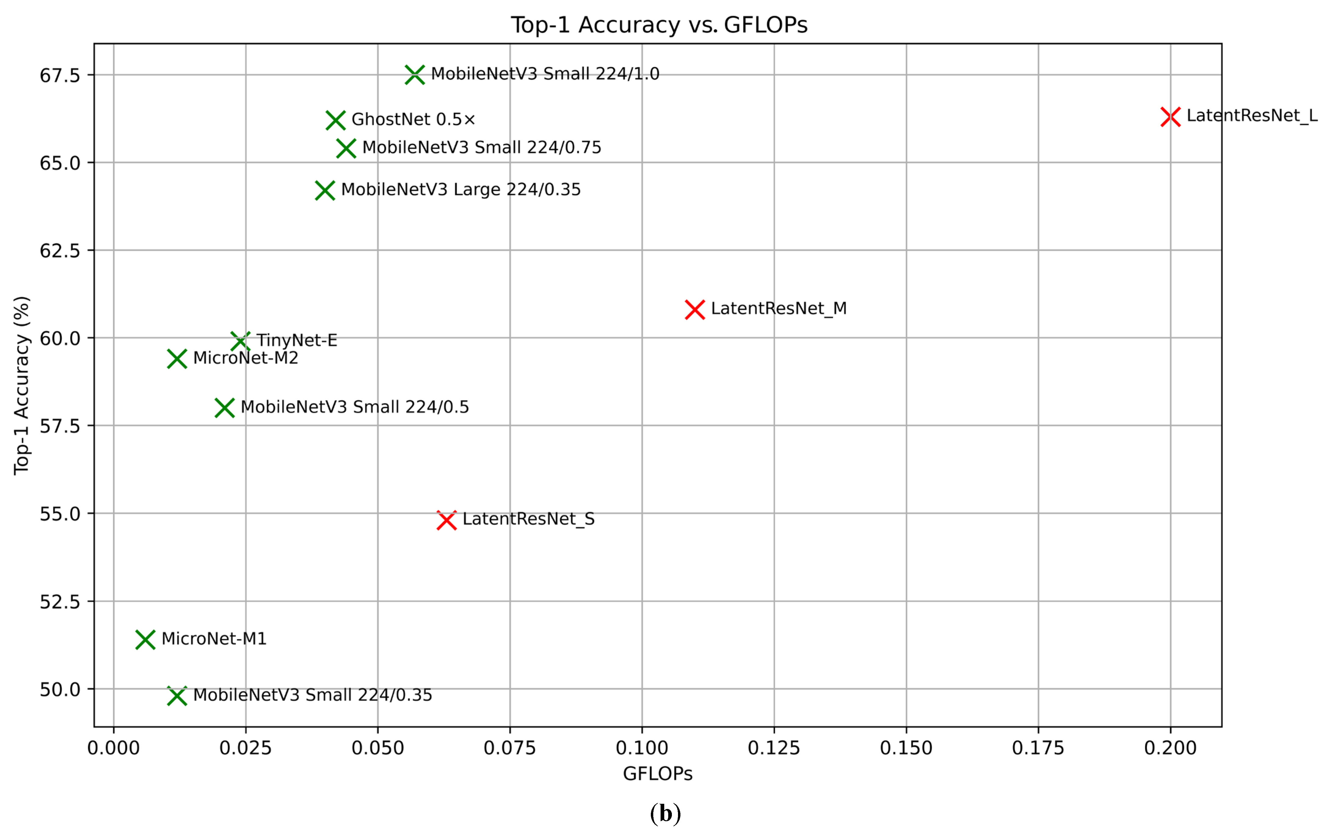
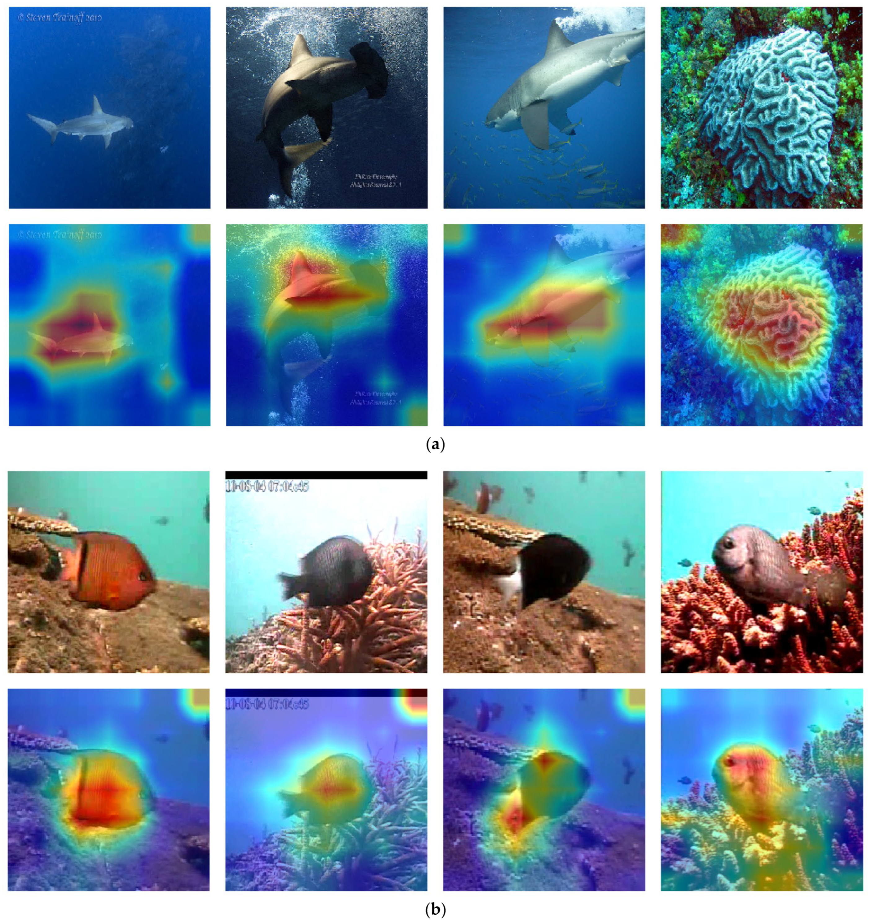
4.2. Experiments on LatentResNet Model

4.2.1. Pretraining and Performance Evaluation on ImageNet-1K Dataset

The model presented in Figure 4 was trained on the ImageNet-1K dataset in two separate scenarios. First, the encoder detailed in Section 3.2 and Section 4.1 was frozen, using the weights previously and independently trained on the same dataset (ImageNet-1K) for the image reconstruction task. In this case, the encoder’s weights were not updated during training for the classification task. In the second scenario, the encoder was fine-tuned, starting from the same pretrained weights that had been trained separately on ImageNet-1K for the image reconstruction task. Table 5 presents the performance of the LatentResNet model with both frozen and unfrozen encoder configurations.
The results show that LatentResNet with an unfrozen encoder outperformed the frozen encoder version, achieving a top-1 accuracy of 66.3%, compared to 65.1% for the frozen version. This can be explained by the ability of the unfrozen encoder to fine-tune its pretrained weights during the next training session for the classification task. While the encoder was pretrained on the same dataset, the nature of its training differed, as it was initially trained specifically for an image reconstruction task. Fine-tuning allows the encoder to adjust its feature representations to better match the specific training objective and the patterns learned by the rest of the network. This process occurs through backpropagation, where gradients guide weight updates in all trainable layers. These updates help the encoder’s features become more effective and improve their interaction with subsequent layers, resulting in better optimization and performance. On the other hand, while the encoder weights obtained during the image reconstruction process on the same dataset were effective for the classification task and provided good training and validation results, the frozen encoder relied on static features, which limited its ability to adapt.
Given the model’s superior top-1 accuracy of 66.3% with an unfrozen encoder, all subsequent experiments will use LatentResNet in this configuration to prioritize performance while maintaining efficiency. This includes the detailed experiments on the underwater fish species classification experiments.
To explore computationally efficient alternatives to the primary LatentResNet model (also referred to as LatentResNet Large), two other versions of the model, as outlined in Section 3.4, were trained. The classification performance and computational costs of these versions are summarized in Table 6, along with a comparison to some well-known lightweight classification models, including MobileNetV3, GhostNet, MicroNet, and TinyNet. Figure 8a shows the relationship between accuracy and the number of parameters, while Figure 8b illustrates the relationship between accuracy and FLOPs, with the LatentResNet variants highlighted in red for better visibility.
LatentResNet_L achieves a 66.3% top-1 accuracy, surpassing MobileNetV3 Large 224/0.35 (64.2%), MobileNetV3-Small 224/0.75 (65.4%), and GhostNet 0.5x (66.2%) while using fewer parameters, with 1.7 million compared to 2.2 million, 2 million, and 2.6 million, respectively. However, it requires higher FLOPs, with 0.2 GFLOPs compared to 0.040 GFLOPs, 0.044 GFLOPs, and 0.042 GFLOPs, respectively. Compared to MobileNetV3 Small 224/1.0, LatentResNet_L uses fewer parameters (1.7M vs. 2.5M) but achieves lower accuracy (66.3% vs. 67.5%) and requires more FLOPs (0.2 GFLOPs vs. 0.057 GFLOPs). LatentResNet_M achieves a 60.8% top-1 accuracy, outperforming MobileNetV3-Small 224/0.5 (58%), TinyNet-E (59.9%), and MicroNet-M2 (59.4%). It uses only 1 million parameters, the lowest among these models, but requires 0.11 GFLOPs, which is higher than the others. LatentResNet_S achieves a 54.8% top-1 accuracy, significantly surpassing MobileNetV3-Small 224/0.35 (49.8%) and MicroNet-M1 (51.4%), while using only 0.7 million parameters compared to 1.4 million and 1.8 million in these models, respectively. However, it requires 0.063 GFLOPs, which is more than both of these benchmark models. The results demonstrate that the LatentResNet variants outperform most of their corresponding lightweight benchmark models in accuracy while using fewer parameters. This makes them well-suited for memory-constrained environments with scalable options to suit different computational budgets. This efficiency comes at the cost of relatively increased computational overhead in terms of FLOPs. Most of these FLOPs come from the DeepResNet blocks, as Table 1 shows that the encoder has very low FLOPs. The LatentResNet variants, although having higher FLOPs than the benchmark models, are still considered to have very low FLOPs, making them suitable for embedded systems and other resource-constrained environments. Additionally, FLOPs can be reduced by using group convolutions in the pointwise part of the separable depthwise layers in DeepResNet blocks, although this will negatively impact the accuracy due to reduced cross-channel interactions.

4.2.2. Fish Species Classification in Underwater Images

After training the LatentResNet model described in Figure 4 and its variants (i.e., medium and small) on ImageNet-1K, the model and its variants were fine-tuned on the Fish4Knowledge dataset. The fine-tuning process employed similar hyperparameters to those described in Section 3.5. Specifically, the Adam optimizer was used with its default settings, except for the learning rate, which was set to 0.0002. A batch size of 32 was used, and early stopping was applied with a patience of 15 epochs based on validation accuracy. As this stage involves fine-tuning, the same architecture of the LatentResNet variants used during training on ImageNet-1K was preserved, including hyperparameters such as the number of filters in each DRB-4 and DRB-2 block, the corresponding spatial dropout configurations, and classic dropout, as detailed in Table 3. However, instead of the 1000 output units used for ImageNet-1K classification (Figure 4), the final dense layer was adjusted to 23 units to match the number of classes in the Fish4Knowledge dataset. The classification metrics and computational costs of the LatentResNet variants and benchmark models trained on the same Fish4Knowledge dataset are reported in Table 7. Additionally, Figure 9 has been included to visually present these results, providing a clearer comparison of the LatentResNet variants’ performance against the benchmark models.
LatentResNet-L, with only 1.39 million parameters and 0.20 GFLOPs, achieves a precision of 99.8%, recall of 99.9%, F1 score of 99.8%, and accuracy of 99.7%. It outperforms existing architectures, including lightweight models, such as MobileNetV2 (with knowledge distillation), CNN-SENet, ConvFishNet, and FishNet in terms of recall, F1 score, and overall classification performance. It also matches ConvFishNet in precision, both achieving 99.8%, while utilizing significantly fewer parameters (1.39 million compared to 14.12 million) and having a lower computational cost (0.20 compared to 0.83 GFLOPs). Compared to MobileNetV2 (with knowledge distillation), which has 2.29 million parameters, FishNet with 16.62 million, and ConvFishNet with 14.12 million, LatentResNet-L offers a significant reduction in model size and computational complexity. Its FLOPs (0.2 FLOPs) are also substantially lower than those of FishNet (4.31 GFLOPs) and ConvFishNet (0.83 GFLOPs). The computational cost of CNN-SENet was not reported in the original study, limiting direct comparison. Nonetheless, these results emphasize LatentResNet-L as a more efficient and higher-performing alternative.
Similarly, LatentResNet-M and LatentResNet-S, with significantly fewer parameters (0.71M and 0.37M, respectively) and lower computational demands (0.11 and 0.06 GFLOPs, respectively), achieved precision scores of 98.8% and 99.3%, F1 scores of 99.0% and 98.9%, and accuracies of 99.8% and 99.7%, respectively. These outcomes outperform FishNet, CNN-SENet, ConvFishNet, and MobileNetV2 in terms of precision (except for ConvFishNet, which achieved 99.8% precision), recall, F1 score, overall reported classification performance, and computational cost. This makes the medium and small variants of LatentResNet especially suitable for extra resource-constrained edge devices. Although LatentResNet-S did not outperform ConvFishNet in terms of precision, it has significantly fewer parameters (0.37M vs. 14.12M) and FLOPs (0.06 vs. 0.83), representing reductions of 97.4% in parameters and 92.8% in FLOPs. This drastic decrease in computational requirements makes LatentResNet-S far more practical for resource-limited applications, despite a marginal precision gap, while still achieving superior recall and F1 score.

4.3. Evaluation of LiteAE and LatentResNet Models’ Performance

The results show that the encoder derived from the autoencoder LiteAE, trained on the ImageNet-1K dataset with an image reconstruction objective, demonstrates significant efficiency when employed as an input in the LatentResNet model for classification tasks. In the context of image reconstruction, the encoder is responsible for compressing high-dimensional input data into a compact latent representation that encapsulates the critical structural and semantic information necessary to regenerate the original image. This encapsulation ultimately leads to a reduction in the computational cost and the number of parameters in the classification model. Furthermore, the features learned through this reconstruction objective demonstrated their inherently general-purpose nature, making them particularly well suited for transfer to other tasks, such as classification.
Generally, using a lightweight autoencoder to compress fish datasets like Fish4Knowledge can be an important step in optimizing data processing and analysis. The Fish4Knowledge dataset consists of large amounts of underwater video and image data, which can be both storage intensive and computationally demanding. By applying a lightweight autoencoder, the size of the data can be effectively reduced while preserving important features. This compression has several benefits. First, it significantly reduces storage and memory usage, which is valuable when working with limited hardware resources or deploying models on edge devices such as autonomous underwater vehicles (AUVs), marine buoys, or remote sensing stations commonly used in marine environments. Second, it speeds up downstream processing tasks such as fish detection, classification, and tracking, as models can operate on compact representations rather than raw data.
The ImageNet-1K dataset was chosen instead of Fish4Knowledge to train LiteAE. This choice offers several advantages. While Fish4Knowledge provides real-world underwater footage that is valuable for domain-specific tasks, it often contains low-resolution and noisy images, which can make it challenging to train accurate and generalizable models. In contrast, ImageNet-1K offers a more diverse, balanced, and high-quality set of labeled images, including several fish-related classes. This makes it a better starting point for training and evaluating general-purpose models, especially when leveraging pretrained architectures for transfer learning.
By capturing a comprehensive and generalized representation of the input data, the encoder trained on image reconstruction can serve as a robust feature extractor when integrated into classification models for downstream tasks such as fish species recognition. The results in Section 4.1 suggest that this generalization capability is particularly evident when the autoencoder is evaluated on unseen data from the same distribution it was trained on. This approach ensures that the learned feature representations are closely aligned with the distribution and characteristics of the target dataset, potentially leading to more effective and relevant performance in downstream tasks such as classification. However, the results also demonstrated higher SSIM performance on the Fish4Knowledge dataset compared to the ImageNet-1K dataset, suggesting that its relatively low complexity compared to other benchmark datasets, shown in Figure 6 and Figure 7, played a significant role. This is likely because Fish4Knowledge lacks the complex, fine-grained details found in datasets such as ImageNet-1K, strawberry, and X-ray. In addition, the presence of fish classes within the ImageNet-1K dataset likely contributed to the model’s effectiveness on the fish-related reconstruction task.
The performance improvements observed in Table 5, where the encoder is fine-tuned rather than frozen when used as input to the classification model, highlight an important insight. Although reconstruction-trained weights capture useful general features, fine-tuning the encoder further enhances its effectiveness for the specific demands of the classification task, resulting in improved performance. This process allows the weights to adapt more precisely, refining the learned representations to better align with the downstream layers of the EncodeResNet model through gradient-based updates.
When considering the computational efficiency, the encoder of LiteAE also contributed to reducing the computational cost, as shown in Table 1, by being designed with lightweight components, such as separable depthwise convolutional and Efficient Channel Attention layers. These layers are computationally efficient while maintaining the capacity to extract meaningful features. Additionally, the encoder effectively compressed the input dimensions from 224 × 224 × 3 to 28 × 28 × 66, significantly reducing the spatial complexity while expanding the depth for richer feature representations. Despite this compression, the encoder retained critical structural and semantic features, as demonstrated by the reconstructed images in Figure 6 and Figure 7 and Table 4, ensuring that the most important features were preserved for downstream tasks like classification. This balance between efficiency and feature retention highlights the suitability of the encoder part of LiteAE in resource-constrained environments for classification tasks, particularly in applications such as fish species recognition, where both accuracy and lightweight deployment are essential.
The DeepResNet blocks used in the LatentResNet model demonstrated a significant ability to refine the features extracted by the encoder when trained on the ImageNet-1K dataset, effectively enhancing the quality of the learned representations for the classification tasks. As highlighted by the results in Table 6, increasing the number of DeepResNet blocks and units consistently improved the model’s performance, with more blocks contributing to higher top-1 accuracy. This trend underscores the role of these blocks in progressively refining and optimizing the feature representations. In addition to their impact on performance, DeepResNet blocks contribute to computational efficiency through their lightweight components. By incorporating separable depthwise convolutional layers and Efficient Channel Attention mechanisms, these blocks effectively balance feature refinement with a reduced computational cost. These design choices make DeepResNet blocks significantly more efficient than traditional ResNet blocks, reducing resource consumption. This efficiency makes them ideal for applications that require high performance while operating under strict computational constraints.
Fine-tuning LatentResNet, initially trained on ImageNet-1K, on the Fish4Knowledge dataset demonstrates superior classification performance. It also maintains a significantly lower computational cost and a reduced model size compared to benchmark models in the literature, as shown in Table 7. This underscores the effectiveness of its lightweight architecture and the advantages of transfer learning in addressing domain-specific challenges such as underwater fish species classification. Interestingly, the results across the large, medium, and small variants of LatentResNet show very similar performances, with only marginal differences in the accuracy, precision, recall, and F1 score. This consistency highlights the efficiency of the smallest variant, LatentResNet_S, which achieves comparable performance (overall accuracy of 99.7%) while offering significant reductions in parameter count and computational cost, with values of 0.37M and 0.06 GFLOPs, respectively. This efficiency is primarily attributed to the architectural design of the LatentResNet variants. The lightweight encoder effectively compresses the input data early in the pipeline, while the subsequent DeepResNet blocks, composed of computationally efficient components such as depthwise separable convolutions, refine the compressed features. Unlike traditional models such as FishNet, CNN-SENet, and ConvFishNet, which rely on standard convolutional layers throughout the architecture, the LatentResNet design significantly reduces both the parameter count and computational cost while achieving superior classification performance. These properties (i.e., efficiency and accuracy performance) make the ultra-lightweight LatentResNet_S well suited for real-time marine monitoring applications, especially in environments with limited computational resources, such as underwater drones, autonomous underwater vehicles, or edge-based marine sensors. Such characteristics are especially critical for enabling scalable and efficient ecological monitoring in aquatic ecosystems, where deployments often rely on resource-constrained platforms operating in real time and under challenging conditions.
To provide insight into the model’s behavior, Score-CAM (Score-Weighted Class Activation Mapping) visualizations were generated for selected input images from the ImageNet-1K and Fish4Knowledge datasets. These visualizations were produced using the final Efficient Channel Attention (ECA) module within the last DeepResNet block of the LatentResNet-L model (Figure 4). This ECA module operates on compressed feature maps of size 7 × 7 with 340 channels, capturing high-level semantic context.
From the ImageNet-1K test set, marine subjects were selected (Figure 10a). In the ImageNet-1K dataset visualizations, the Score-CAM heatmaps highlight the main objects in each scene, focusing on regions with distinctive shapes and textures that are crucial for the model’s classification. For example, in the hammerhead shark image (Figure 10a), the heatmap concentrates on the head and upper body, effectively capturing the distinctive hammer shape. Similarly, in the coral image (Figure 10a), the heatmap focuses on the coral’s central structure, highlighting its textured ridges as the primary class-relevant feature.
In the Fish4Knowledge dataset (Figure 10b), the heatmaps emphasize the fish bodies amidst coral environments, even in the presence of lower image quality and underwater noise. The model shows attention to specific body features like the silhouette and fins, which are key for classification. For instance, in the left-most image (Figure 10b), the heatmap generated by Score-CAM distinctly highlights its body and fins. Despite the presence of coral structures, the model successfully identifies the main features of the fish, such as its silhouette and fin structure, which are crucial for recognizing its class. Similarly, in the right-most image (Figure 10b), the model again prioritizes the fish’s body and head regions in the heatmap. Even with visual noise and complex coral textures surrounding it, the model is still able to pinpoint the primary features of the fish for classification.
These observations across both datasets indicate that the model effectively identifies class-salient regions, prioritizing the overall shapes and structural details for robust classification across diverse images, even in the presence of variations in quality and underwater visual noise.

5. Conclusions

In this paper, a lightweight autoencoder named LiteAE and a classification model called LatentResNet are presented for fish species recognition. The proposed LiteAE demonstrated strong efficiency in reconstructing input images despite its lightweight design, particularly on the Fish4Knowledge dataset; however, a slight blur in the reconstructed images suggests difficulty in capturing the most intricate details. The LatentResNet model consists of two major components: the encoder part of the proposed LiteAE applied to the input and the proposed DeepResNet blocks, which refine the features extracted by the encoder. The encoder of LiteAE plays a crucial role in reducing the computational cost of the LatentResNet model by compressing the input data into a lower spatial dimension. On the other hand, the DeepResNet block, inspired by the ResNet block, utilizes components with lower computational costs, such as depthwise separable layers and Efficient Channel Attention (ECA), compared to the standard ResNet block.
Lighter-scaled versions of the LatentResNet model, named medium and small, were developed by consistently reducing the number of DeepResNet blocks and units, while the large version serves as the base model. This approach provides more efficient options for environments with stricter constraints on power, memory, and computational resources. Experiments conducted on the LatentResNet classification model and its variants on ImageNet-1K dataset demonstrated higher top-1 accuracy and reduced parameter counts compared to benchmark models designed for similar computational objectives. This performance was achieved while maintaining relatively low FLOPs, despite being higher than those of the benchmark models. Fine-tuning the LatentResNet model, initially trained on the ImageNet-1K dataset, on the Fish4Knowledge fish species dataset resulted in improved performance compared to benchmark models trained and evaluated on the same dataset. The fine-tuned model generally achieved higher precision, recall, F1 score, and accuracy, along with significant reductions in parameters and FLOPs, reaching up to 97.4% and 92.8%, respectively, compared to the benchmark models. The results demonstrate the effectiveness of using the encoder part of an autoencoder, trained on an image reconstruction task, as input to a classification model for complex classification tasks, particularly with challenging datasets like ImageNet-1K and Fish4Knowledge. This approach proved to be effective in reducing the FLOPs and parameters while maintaining strong accuracy performance, making it a practical solution for marine classification tasks that require a low model size and computational cost. This is especially important in real-time underwater monitoring scenarios, where computational resources are limited, such as on underwater drones, autonomous underwater vehicles (AUVs), or edge-based marine sensors. The compact size and low computational demand of LatentResNet enable scalable and energy-efficient deployment in challenging aquatic environments. As a result, it supports continuous and widespread ecological monitoring, helping researchers and conservationists gather actionable insights from remote or sensitive marine ecosystems without relying on high-powered infrastructure.
In future work, the performance of LatentResNet variants will be evaluated on various marine-related tasks beyond species classification, such as underwater object detection, fish counting, and anomaly detection. Additionally, the proposed model variants will be deployed on actual edge devices (e.g., Jetson Nano and Raspberry Pi) to assess their real-time latency performance in practical settings and facilitate latency comparisons with benchmark models.

Author Contributions

The authors contributed to this research as follows: M.H. contributed to Conceptualization, Methodology, Software, and Writing—original draft; E.A. contributed to Conceptualization, Resources, Writing—review and editing, and Supervision; and A.A. contributed to Writing—review and editing and Supervision. All authors have read and agreed to the published version of the manuscript.

Funding

This research received no external funding.

Data Availability Statement

The datasets presented in this study are openly available. The ImageNet-1K dataset is available at https://doi.org/10.1109/CVPR.2009.5206848. This reference is provided here for context and is not included in the main References section. The Fish4Knowledge dataset is available at https://doi.org/10.1007/978-3-319-30208-9 and is cited in the References section as reference number [40].

Acknowledgments

During the preparation of this manuscript, the authors used GPT-4o for language refinement, grammar correction, and improving the clarity of expression. The tool was not used to generate scientific content, results, or data analysis. The scientific content, experimental design, data analysis, and interpretations throughout the manuscript, including Materials and Methods, were entirely authored and validated by the researchers. All outputs generated using the tool were thoroughly reviewed and edited by the authors. The authors take full responsibility for the content of this publication.

Conflicts of Interest

The authors declare no conflict of interest.

References

  1. Woo, S.; Debnath, S.; Hu, R.; Chen, X.; Liu, Z.; Kweon, I.S.; Xie, S. Convnext v2: Co-designing and scaling convnets with masked autoencoders. In Proceedings of the IEEE/CVF Conference on Computer Vision and Pattern Recognition, Vancouver, BC, Canada, 17–24 June 2023; pp. 16133–16142. [Google Scholar]
  2. Park, S.; Byun, H. Fair-VPT: Fair Visual Prompt Tuning for Image Classification. In Proceedings of the IEEE/CVF Conference on Computer Vision and Pattern Recognition, Seattle, WA, USA, 16–22 June 2024; pp. 12268–12278. [Google Scholar]
  3. Hariri, M.; Aydın, A.; Sıbıç, O.; Somuncu, E.; Yılmaz, S.; Sönmez, S.; Avşar, E. LesionScanNet: Dual-path convolutional neural network for acute appendicitis diagnosis. Health Inf. Sci. Syst. 2025, 13, 3. [Google Scholar] [CrossRef] [PubMed]
  4. Zhou, Y. A YOLO-NL object detector for real-time detection. Expert Syst. Appl. 2024, 238, 122256. [Google Scholar] [CrossRef]
  5. Chen, S.; Sun, P.; Song, Y.; Luo, P. Diffusiondet: Diffusion model for object detection. In Proceedings of the IEEE/CVF International Conference on Computer Vision, Paris, France, 1–6 October 2023; pp. 19830–19843. [Google Scholar]
  6. Wang, A.; Chen, H.; Liu, L.; Chen, K.; Lin, Z.; Han, J. Yolov10: Real-time end-to-end object detection. Adv. Neural Inf. Process. Syst. 2024, 37, 107984–108011. [Google Scholar]
  7. Xiong, Y.; Varadarajan, B.; Wu, L.; Xiang, X.; Xiao, F.; Zhu, C.; Dai, X.; Wang, D.; Sun, F.; Iandola, F. Efficientsam: Leveraged masked image pretraining for efficient segment anything. In Proceedings of the IEEE/CVF Conference on Computer Vision and Pattern Recognition, Seattle, WA, USA, 16–22 June 2024; pp. 16111–16121. [Google Scholar]
  8. Kirillov, A.; Mintun, E.; Ravi, N.; Mao, H.; Rolland, C.; Gustafson, L.; Xiao, T.; Whitehead, S.; Berg, A.C.; Lo, W.-Y. Segment anything. In Proceedings of the IEEE/CVF International Conference on Computer Vision, Paris, France, 1–6 October 2023; pp. 4015–4026. [Google Scholar]
  9. Zou, X.; Yang, J.; Zhang, H.; Li, F.; Li, L.; Wang, J.; Wang, L.; Gao, J.; Lee, Y.J. Segment everything everywhere all at once. Adv. Neural Inf. Process. Syst. 2023, 36, 19769–19782. [Google Scholar]
  10. Weinbach, B.C.; Akerkar, R.; Nilsen, M.; Arghandeh, R. Hierarchical deep learning framework for automated marine vegetation and fauna analysis using ROV video data. Ecol. Inform. 2025, 85, 102966. [Google Scholar] [CrossRef]
  11. Malik, H.; Naeem, A.; Hassan, S.; Ali, F.; Naqvi, R.A.; Yon, D.K. Multi-classification deep neural networks for identification of fish species using camera captured images. PLoS ONE 2023, 18, e0284992. [Google Scholar] [CrossRef]
  12. Lowe, S.C.; Misiuk, B.; Xu, I.; Abdulazizov, S.; Baroi, A.R.; Bastos, A.C.; Best, M.; Ferrini, V.; Friedman, A.; Hart, D. BenthicNet: A global compilation of seafloor images for deep learning applications. Sci. Data 2025, 12, 230. [Google Scholar] [CrossRef]
  13. Wang, B.; Hua, L.; Mei, H.; Kang, Y.; Zhao, N. Monitoring marine pollution for carbon neutrality through a deep learning method with multi-source data fusion. Front. Ecol. Evol. 2023, 11, 1257542. [Google Scholar] [CrossRef]
  14. Li, Y.; Liu, J.; Kusy, B.; Marchant, R.; Do, B.; Merz, T.; Crosswell, J.; Steven, A.; Tychsen-Smith, L.; Ahmedt-Aristizabal, D. A real-time edge-AI system for reef surveys. In Proceedings of the 28th Annual International Conference on Mobile Computing And Networking, Sydney, NSW, Australia, 17–21 October 2022; pp. 903–906. [Google Scholar]
  15. Avsar, E.; Feekings, J.P.; Krag, L.A. Edge computing based real-time Nephrops (Nephrops norvegicus) catch estimation in demersal trawls using object detection models. Sci. Rep. 2024, 14, 9481. [Google Scholar] [CrossRef]
  16. Lu, Z.; Liao, L.; Xie, X.; Yuan, H. SCoralDet: Efficient real-time underwater soft coral detection with YOLO. Ecol. Inform. 2025, 85, 102937. [Google Scholar] [CrossRef]
  17. He, K.; Zhang, X.; Ren, S.; Sun, J. Deep residual learning for image recognition. In Proceedings of the IEEE Conference on Computer Vision and Pattern Recognition, Las Vegas, NV, USA, 27–30 June 2016; pp. 770–778. [Google Scholar]
  18. Chollet, F. Xception: Deep learning with depthwise separable convolutions. In Proceedings of the IEEE Conference on Computer Vision and Pattern Recognition, Honolulu, Hi, USA, 21–26 July 2017; pp. 1251–1258. [Google Scholar]
  19. Xie, S.; Girshick, R.; Dollár, P.; Tu, Z.; He, K. Aggregated residual transformations for deep neural networks. In Proceedings of the IEEE Conference on Computer Vision and Pattern Recognition, Honolulu, Hi, USA, 21–26 July 2017; pp. 1492–1500. [Google Scholar]
  20. Pham, H.; Guan, M.; Zoph, B.; Le, Q.; Dean, J. Efficient neural architecture search via parameters sharing. In Proceedings of the International Conference on Machine Learning, Stockholm, Sweden, 10–15 July 2018; pp. 4095–4104. [Google Scholar]
  21. Kamath, V.; Renuka, A. Deep learning based object detection for resource constrained devices: Systematic review, future trends and challenges ahead. Neurocomputing 2023, 531, 34–60. [Google Scholar] [CrossRef]
  22. Howard, A.; Zhu, M.; Chen, B.; Kalenichenko, D.; Wang, W.; Weyand, T.; Andreetto, M.; Adam, H. MobileNets: Efficient Convolutional Neural Networks for Mobile Vision Applications. arXiv 2017, arXiv:1704.04861. [Google Scholar]
  23. Sandler, M.; Howard, A.; Zhu, M.; Zhmoginov, A.; Chen, L.-C. Mobilenetv2: Inverted residuals and linear bottlenecks. In Proceedings of the IEEE Conference on Computer Vision and Pattern Recognition, Salt Lake City, UT, USA, 18–23 June 2018; pp. 4510–4520. [Google Scholar]
  24. Howard, A.; Sandler, M.; Chu, G.; Chen, L.-C.; Chen, B.; Tan, M.; Wang, W.; Zhu, Y.; Pang, R.; Vasudevan, V. Searching for mobilenetv3. In Proceedings of the IEEE/CVF International Conference on Computer Vision, Seoul, Republic of Korea, 27 October–2 November 2019; pp. 1314–1324. [Google Scholar]
  25. Tan, M.; Le, Q. Efficientnet: Rethinking model scaling for convolutional neural networks. In Proceedings of the International Conference on Machine Learning, Long Beach, CA, USA, 9–15 June 2019; pp. 6105–6114. [Google Scholar]
  26. Han, K.; Wang, Y.; Tian, Q.; Guo, J.; Xu, C.; Xu, C. Ghostnet: More features from cheap operations. In Proceedings of the IEEE/CVF Conference on Computer Vision and Pattern Recognition, Seattle, WA, USA, 13–19 June 2020; pp. 1580–1589. [Google Scholar]
  27. Radosavovic, I.; Kosaraju, R.P.; Girshick, R.; He, K.; Dollár, P. Designing network design spaces. In Proceedings of the IEEE/CVF Conference on Computer Vision and Pattern Recognition, Seattle, WA, USA, 13–19 June 2020; pp. 10428–10436. [Google Scholar]
  28. Maaz, M.; Shaker, A.; Cholakkal, H.; Khan, S.; Zamir, S.W.; Anwer, R.M.; Shahbaz Khan, F. Edgenext: Efficiently amalgamated cnn-transformer architecture for mobile vision applications. In Proceedings of the European Conference on Computer Vision, Tel Aviv, Israel, 23–27 October 2022; pp. 3–20. [Google Scholar]
  29. Mehta, S.; Rastegari, M. Mobilevit: Light-weight, general-purpose, and mobile-friendly vision transformer. arXiv 2021, arXiv:2110.02178. [Google Scholar]
  30. Chen, Y.; Wang, Z. An effective information theoretic framework for channel pruning. arXiv 2024, arXiv:2408.16772. [Google Scholar]
  31. Liu, J.; Tang, D.; Huang, Y.; Zhang, L.; Zeng, X.; Li, D.; Lu, M.; Peng, J.; Wang, Y.; Jiang, F. Updp: A unified progressive depth pruner for cnn and vision transformer. In Proceedings of the AAAI Conference on Artificial Intelligence, Vancouver, BC, Canada, 20–27 February 2024; pp. 13891–13899. [Google Scholar]
  32. Xu, K.; Wang, Z.; Chen, C.; Geng, X.; Lin, J.; Yang, X.; Wu, M.; Li, X.; Lin, W. Lpvit: Low-power semi-structured pruning for vision transformers. In Proceedings of the European Conference on Computer Vision, Milan, Italy, 29 September–4 October 2024; pp. 269–287. [Google Scholar]
  33. Choi, K.; Lee, H.Y.; Kwon, D.; Park, S.; Kim, K.; Park, N.; Lee, J. MimiQ: Low-Bit Data-Free Quantization of Vision Transformers. arXiv 2024, arXiv:2407.20021. [Google Scholar]
  34. Shi, H.; Cheng, X.; Mao, W.; Wang, Z. P $^ 2$-ViT: Power-of-Two Post-Training Quantization and Acceleration for Fully Quantized Vision Transformer. IEEE Trans. Very Large Scale Integr. VLSI Syst. 2024, 32, 1704–1717. [Google Scholar] [CrossRef]
  35. Ding, R.; Yong, L.; Zhao, S.; Nie, J.; Chen, L.; Liu, H.; Zhou, X. Progressive Fine-to-Coarse Reconstruction for Accurate Low-Bit Post-Training Quantization in Vision Transformers. arXiv 2024, arXiv:2412.14633. [Google Scholar] [CrossRef] [PubMed]
  36. Wang, J.; Chen, Y.; Zheng, Z.; Li, X.; Cheng, M.-M.; Hou, Q. CrossKD: Cross-head knowledge distillation for object detection. In Proceedings of the IEEE/CVF Conference on Computer Vision and Pattern Recognition, Seattle, WA, USA, 16–22 June 2024; pp. 16520–16530. [Google Scholar]
  37. Salie, D.; Brown, D.; Chieza, K. Deep Neural Network Compression for Lightweight and Accurate Fish Classification. In Proceedings of the Southern African Conference for Artificial Intelligence Research, Bloemfontein, South Africa, 2–6 December 2024; pp. 300–318. [Google Scholar]
  38. Sun, S.; Ren, W.; Li, J.; Wang, R.; Cao, X. Logit standardization in knowledge distillation. In Proceedings of the IEEE/CVF Conference on Computer Vision and Pattern Recognition, Seattle, WA, USA, 16–22 June 2024; pp. 15731–15740. [Google Scholar]
  39. Wu, B.; Dai, X.; Zhang, P.; Wang, Y.; Sun, F.; Wu, Y.; Tian, Y.; Vajda, P.; Jia, Y.; Keutzer, K. Fbnet: Hardware-aware efficient convnet design via differentiable neural architecture search. In Proceedings of the IEEE/CVF Conference on Computer Vision and Pattern Recognition, Seattle, WA, USA, 16–22 June 2024; pp. 10734–10742. [Google Scholar]
  40. Tan, M.; Le, Q. Efficientnetv2: Smaller models and faster training. arXiv 2021, arXiv:2104.00298. [Google Scholar]
  41. Sharma, K.; Gupta, S.; Rameshan, R. Learning optimally separated class-specific subspace representations using convolutional autoencoder. arXiv 2021, arXiv:2105.08865. [Google Scholar]
  42. Gogna, A.; Majumdar, A. Discriminative autoencoder for feature extraction: Application to character recognition. Neural Process. Lett. 2019, 49, 1723–1735. [Google Scholar] [CrossRef]
  43. Kong, Q.; Chiang, A.; Aguiar, A.C.; Fernández-Godino, M.G.; Myers, S.C.; Lucas, D.D. Deep convolutional autoencoders as generic feature extractors in seismological applications. Artif. Intell. Geosci. 2021, 2, 96–106. [Google Scholar] [CrossRef]
  44. Fisher, R.B.; Chen-Burger, Y.-H.; Giordano, D.; Hardman, L.; Lin, F.-P. Fish4Knowledge: Collecting and Analyzing Massive Coral Reef Fish Video Data; Springer: Berlin/Heidelberg, Germany, 2016; Volume 104. [Google Scholar]
  45. Hinton, G.E.; Zemel, R. Autoencoders, minimum description length and Helmholtz free energy. Adv. Neural Inf. Process. Syst. 1993, 6, 3–10. [Google Scholar]
  46. Tompson, J.; Goroshin, R.; Jain, A.; LeCun, Y.; Bregler, C. Efficient object localization using convolutional networks. In Proceedings of the IEEE Conference on Computer Vision and Pattern Recognition, Boston, MA, USA, 7–12 June 2015; pp. 648–656. [Google Scholar]
  47. Wang, Q.; Wu, B.; Zhu, P.; Li, P.; Zuo, W.; Hu, Q. ECA-Net: Efficient channel attention for deep convolutional neural networks. In Proceedings of the IEEE/CVF Conference on Computer Vision and Pattern Recognition, Seattle, WA, USA, 13–19 June 2020; pp. 11534–11542. [Google Scholar]
  48. Shen, F.; Gan, R.; Zeng, G. Weighted residuals for very deep networks. In Proceedings of the 2016 3rd International Conference on Systems and Informatics (ICSAI), Shanghai, China, 19–21 November 2016; pp. 936–941. [Google Scholar]
  49. Hendrycks, D.; Gimpel, K. Gaussian error linear units (gelus). arXiv 2016, arXiv:1606.08415. [Google Scholar]
  50. Wang, Z.; Bovik, A.C.; Sheikh, H.R.; Simoncelli, E.P. Image quality assessment: From error visibility to structural similarity. IEEE Trans. Image Process. 2004, 13, 600–612. [Google Scholar] [CrossRef] [PubMed]
  51. DTU Computing Center. DTU Computing Center Resources; DTU Computing Center: Lyngby, Denmark, 2024. [Google Scholar]
  52. Sait, U.; Lal, K.; Prajapati, S.; Bhaumik, R.; Kumar, T.; Sanjana, S.; Bhalla, K. Curated dataset for COVID-19 posterior-anterior chest radiography images (X-Rays). Mendeley Data 2020, 1. [Google Scholar] [CrossRef]
  53. Hariri, M.; Avşar, E. Tipburn disorder detection in strawberry leaves using convolutional neural networks and particle swarm optimization. Multimed. Tools Appl. 2022, 81, 11795–11822. [Google Scholar] [CrossRef]
  54. Han, K.; Wang, Y.; Zhang, Q.; Zhang, W.; Xu, C.; Zhang, T. Model Rubik’s cube: Twisting resolution, depth and width for tinynets. Adv. Neural Inf. Process. Syst. 2020, 33, 19353–19364. [Google Scholar]
  55. Li, Y.; Chen, Y.; Dai, X.; Chen, D.; Liu, M.; Yuan, L.; Liu, Z.; Zhang, L.; Vasconcelos, N. Micronet: Improving image recognition with extremely low flops. In Proceedings of the IEEE/CVF International Conference on Computer Vision, Montreal, QC, Canada, 10–17 October 2021; pp. 468–477. [Google Scholar]
  56. Sun, S.; Pang, J.; Shi, J.; Yi, S.; Ouyang, W. Fishnet: A versatile backbone for image, region, and pixel level prediction. Adv. Neural Inf. Process. Syst. 2018, 31, 1–11. [Google Scholar]
  57. Knausgård, K.M.; Wiklund, A.; Sørdalen, T.K.; Halvorsen, K.T.; Kleiven, A.R.; Jiao, L.; Goodwin, M. Temperate fish detection and classification: A deep learning based approach. Appl. Intell. 2022, 52, 6988–7001. [Google Scholar] [CrossRef]
  58. Qu, H.; Wang, G.-G.; Li, Y.; Qi, X.; Zhang, M. ConvFishNet: An efficient backbone for fish classification from composited underwater images. Inf. Sci. 2024, 679, 121078. [Google Scholar] [CrossRef]
Figure 1. Three samples from the Fish4Knowledge dataset.
Jmse 13 01019 g001
Figure 2. The structure of the proposed autoencoder LiteAE.
Jmse 13 01019 g002
Figure 3. The architecture of the proposed DeepResNet Unit (a) and the variants of DeepResNet block, DRB-2 (b) and DRB-4 (c).
Jmse 13 01019 g003
Figure 4. The structure of the proposed LatentResNet-L model. Blocks with the same color perform the same type of operation.
Jmse 13 01019 g004
Figure 5. Training and evaluation pipeline for LatentResNet variants using ImageNet-1K and Fish4Knowledge datasets.
Jmse 13 01019 g005
Figure 6. The input (top) and reconstructed images (bottom) generated by the autoencoder using the test subset of ImageNet-1K dataset.
Jmse 13 01019 g006
Figure 7. The input (top row) and reconstructed images (bottom row) generated by the autoencoder LiteAE using the underwater fish (a), X-ray (b), and strawberry leaf (c) datasets.
Jmse 13 01019 g007aJmse 13 01019 g007b
Figure 8. The relationship between accuracy and parameter count (a) and accuracy and GFLOPs (b) for LatentResNet variants and benchmark models. The values belonging to the LatentResNet and remaining models are given in red and green, respectively.
Jmse 13 01019 g008aJmse 13 01019 g008b
Figure 9. Visual comparison of classification metrics between the proposed LatentResNet variants and benchmark models on the Fish4Knowledge dataset.
Jmse 13 01019 g009
Figure 10. Score-CAM visualizations for samples from the ImageNet-1K dataset (a) and the Fish4Knowledge dataset (b), where the first row represents the input images, and the second row displays the corresponding Score-CAM visualizations.
Jmse 13 01019 g010
Table 1. The computational cost metrics associated with the encoder and decoder parts of the LiteAE.
GFLOPsNumber of Parameters (Millions)
Encoder0.010.006
Decoder0.370.088
Table 2. Data augmentation techniques applied during training.
Augmentation NameRange/Parameters (Random)
ShearShear angle: [−0.25, 0.25] (radians)
TranslateWidth: [0%, 25%]; height: [0%, 25%] of image size
ZoomZoom factor: [0.75, 1.25]
Flip (horizontal)-
RotateRotation angle: [−0.35, 0.35] radians
Brightness adjustmentΔ ∈ [0.06, 0.14] to pixel values
Channel shiftShift: [−0.196, 0.196] (normalized from pixel range [−50, 50])
Random crop + padCrop: 160 × 160, then pad to 224 × 224
Random black rectangleHeight: [45, 60]; width: [80, 100]; position: random
Table 3. Architectural hyperparameters for different LatentResNet model variants.
Number of FiltersSpatial Dropout RateClassic Dropout Rate
1st Pair of DeepResNet Blocks2nd Pair of DeepResNet Blocks3rd Pair of DeepResNet Blocks
LatentResNet-L1101803400.020.1
LatentResNet-M0.010.05
LatentResNet-S0.0050.05
Table 4. The quantitative performance metrics of the autoencoder LiteAE.
DatasetSSIMPSNR (dB)MSE
Imagnet1k test data0.750823.150.0067
Fish4Knowledge dataset0.843622.980.0053
X-ray dataset0.720021.830.0049
Strawberry dataset0.719323.400.0069
Table 5. The performance of the LatentResNet model with frozen and unfrozen encoder configurations.
ModelLatentResNetLatentResNet (Frozen Encoder)
Top-1 accuracy66.3%65.1%
Table 6. The classification performance, computational costs, and number of parameters for different LatentResNet and some state-of-the-art lightweight models. The best values are given in bold.
ModelTop-1 AccuracyGFLOPsNumber of Parameters (M)
MobileNetV3 Large 224/0.35 [24]64.2%0.0402.2
MobileNetV3 Small 224/1.0 [24]67.5%0.0572.5
MobileNetV3 Small 224/0.75 [24]65.4%0.0442.0
GhostNet 0.5× [26]66.2%0.0422.6
LatentResNet_L66.3%0.2001.7
MobileNetV3 Small 224/0.5 [24]58.0%0.0211.6
TinyNet-E [54]59.9%0.0242.0
MicroNet-M2 [55]59.4%0.0122.4
LatentResNet_M60.8%0.1101.0
MobileNetV3 Small 224/0.35 [24]49.8%0.0121.4
MicroNet-M1 [55]51.4%0.0061.8
LatentResNet_S54.8%0.0630.7
Table 7. The performance and computational cost of LatentResNet variants against benchmark models trained on the Fish4Knowledge dataset. The best values are given in bold.
ModelParameters
(M)
GFLOPsMacro-AveragesAccuracy
(%)
Precision
(%)
Recall
(%)
F1 Score
(%)
FishNet [56]16.624.3196.888.392.3-
CNN-SENet [57]--97.495.396.099.3
ConvFishNet [58]14.120.8399.897.598.6-
MobileNetV2 (knowledge distillation) [37]2.29-97.782.789.696.6
LatentResNet_L1.390.2099.899.999.999.7
LatentResNet_M0.710.1198.899.499.099.8
LatentResNet_S0.370.0699.398.698.999.7
Disclaimer/Publisher’s Note: The statements, opinions and data contained in all publications are solely those of the individual author(s) and contributor(s) and not of MDPI and/or the editor(s). MDPI and/or the editor(s) disclaim responsibility for any injury to people or property resulting from any ideas, methods, instructions or products referred to in the content.

