
Zero-Vector-Free MPC with Virtual Vector Synthesis for CMV Suppression in Electric Propulsion Systems


Abstract
1. Introduction
- Introducing a zero-vector-free MPC strategy using virtual vector synthesis.
- Achieving CMV suppression without output performance degradation.
- Maintaining low computational complexity suitable for real-time marine applications.
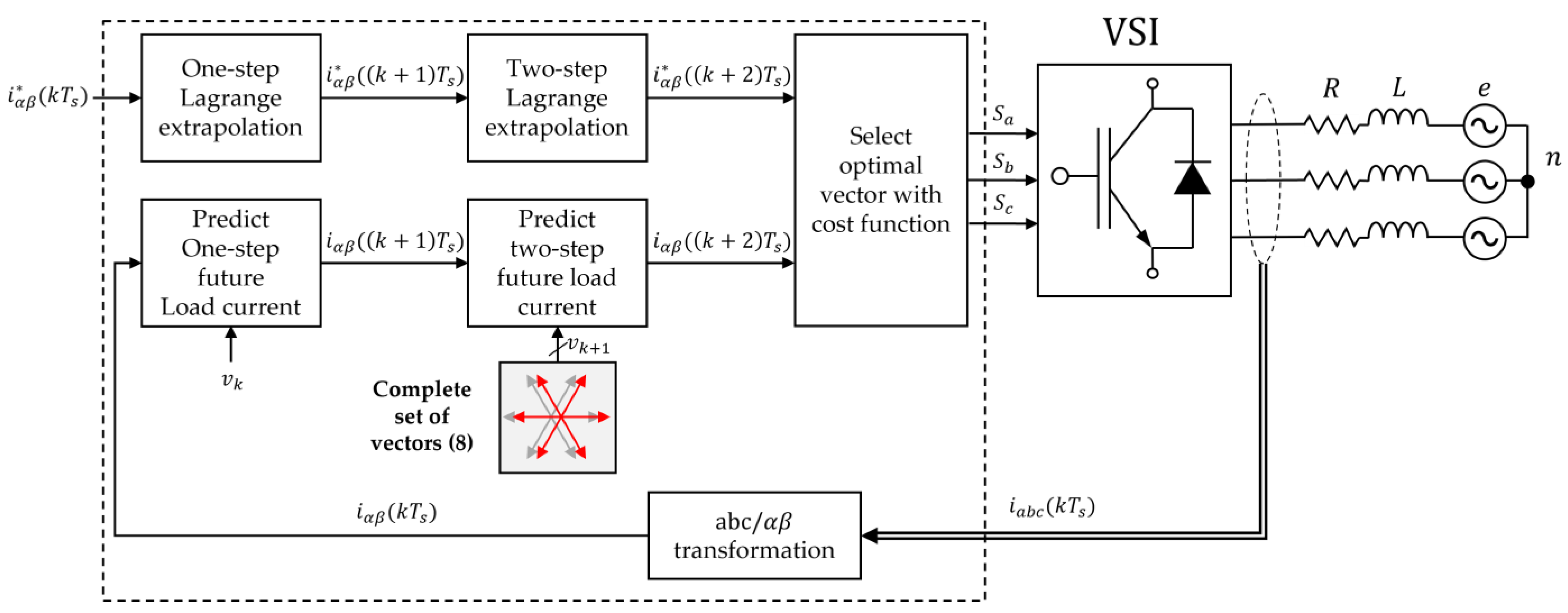
2. Conventional Model Predictive Control
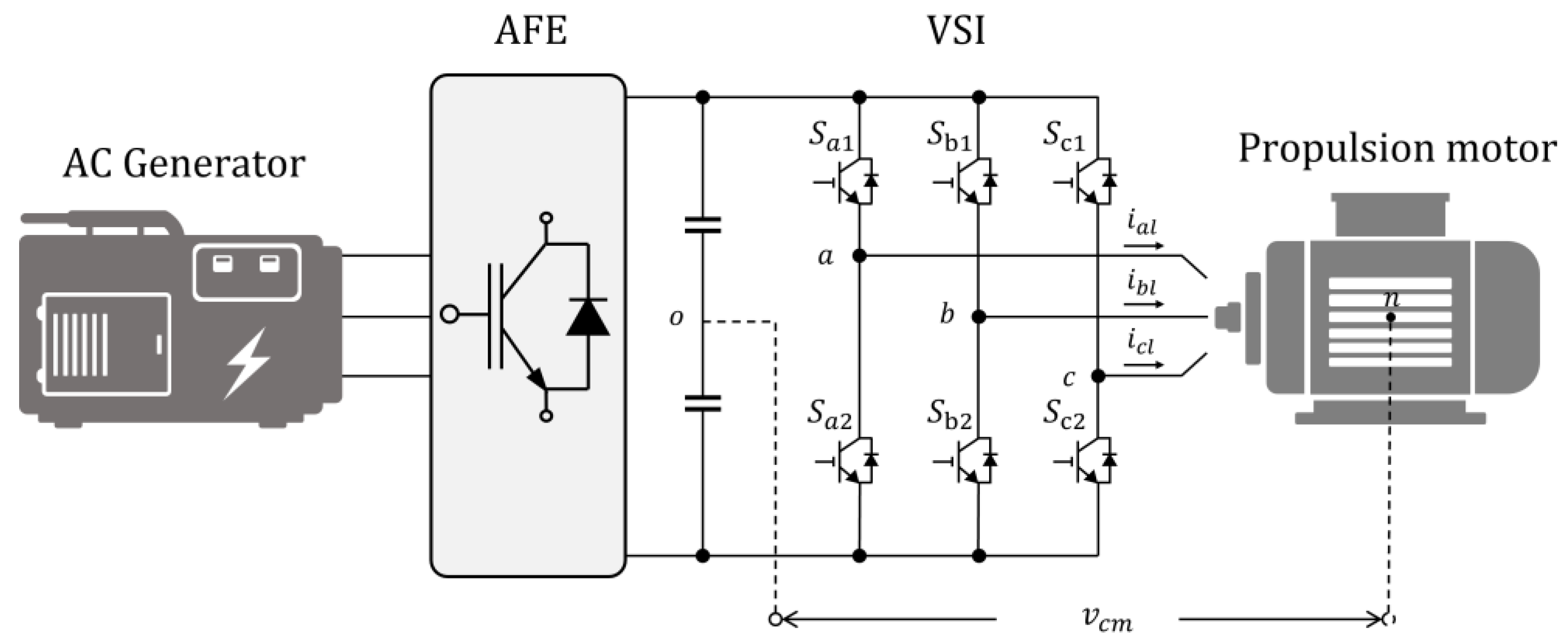
2.1. Three-Phase Voltage Source Inverter
2.2. Model Predictive Control
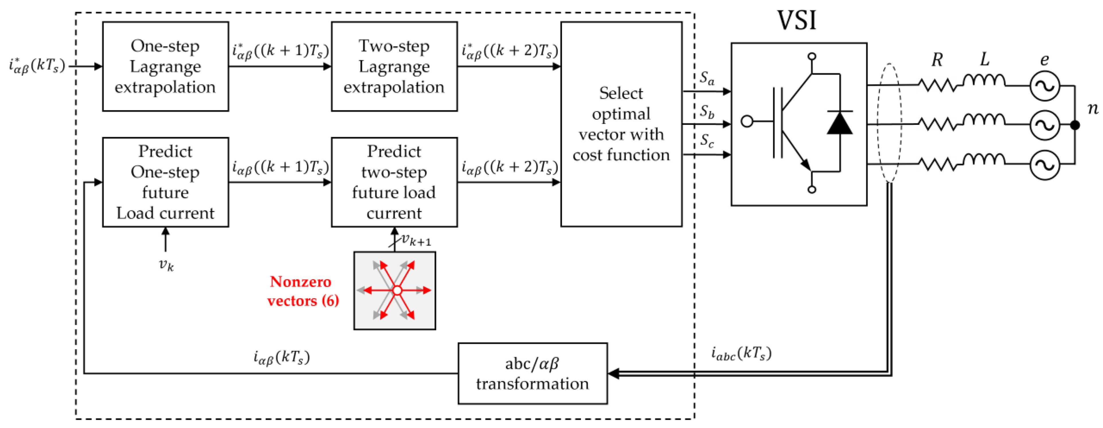
2.3. Reduced Common-Mode Voltage MPC
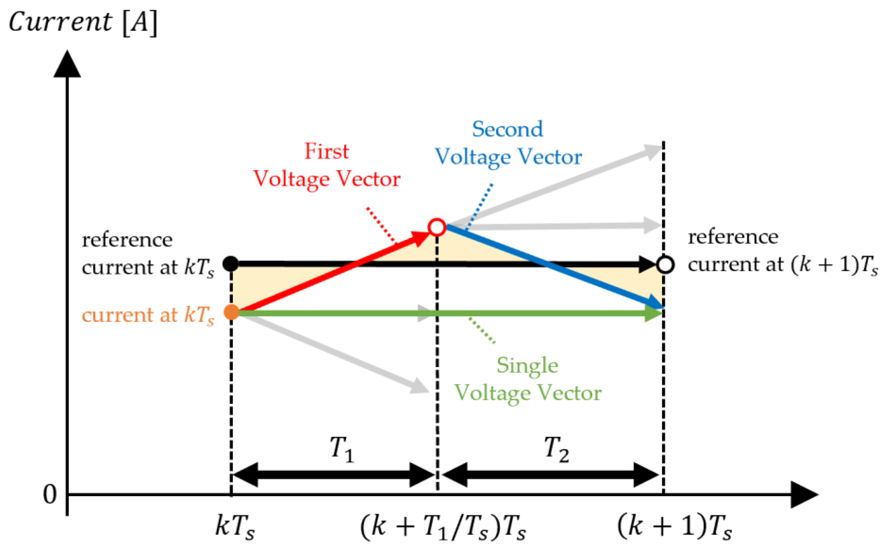
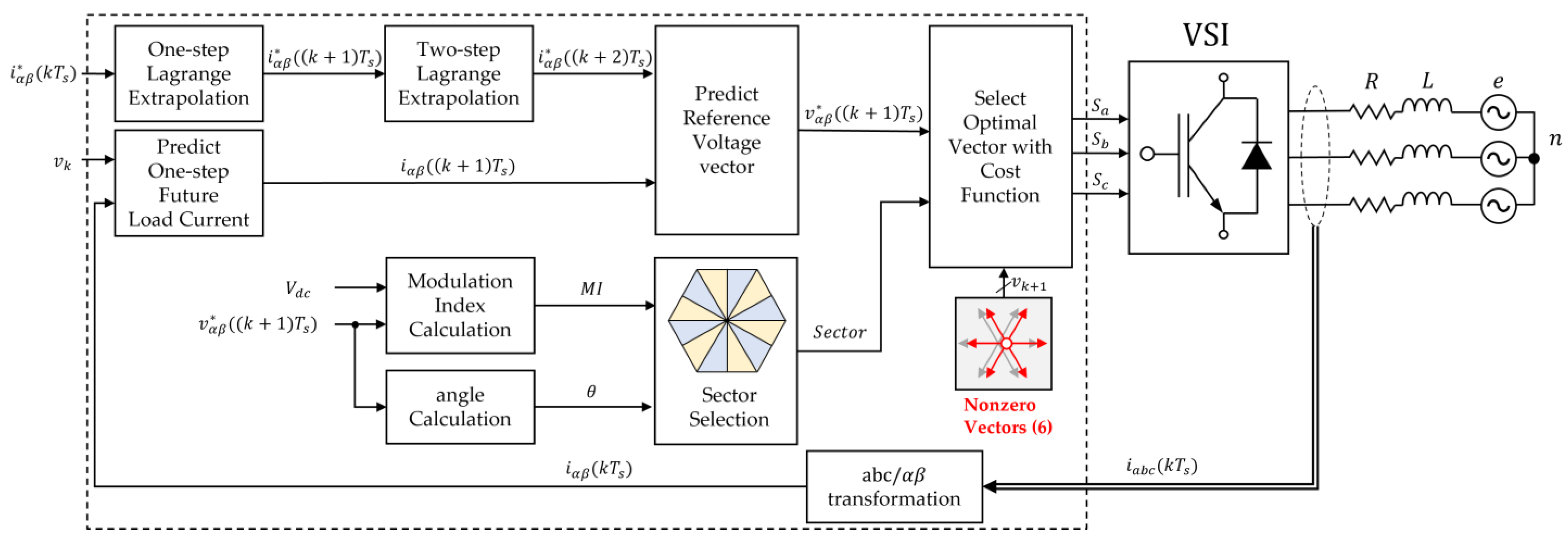
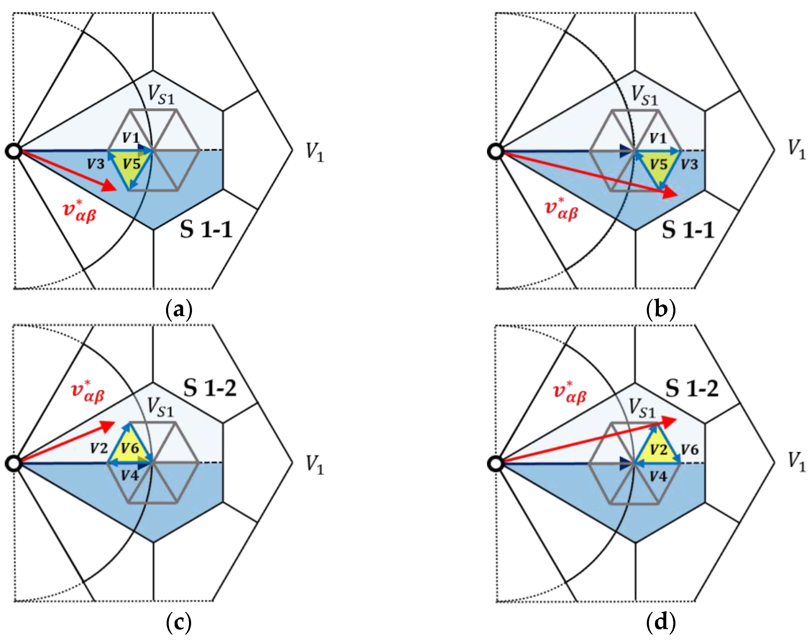
3. Proposed Virtual Multi-Vector Based RCMV-MPC
- Vector selection strategy:
- Zero-vector handling:
- Voltage resolution and tracking accuracy:
- Current quality (ripple and THD):
- Switching frequency and implementation complexity:
- Computational burden:
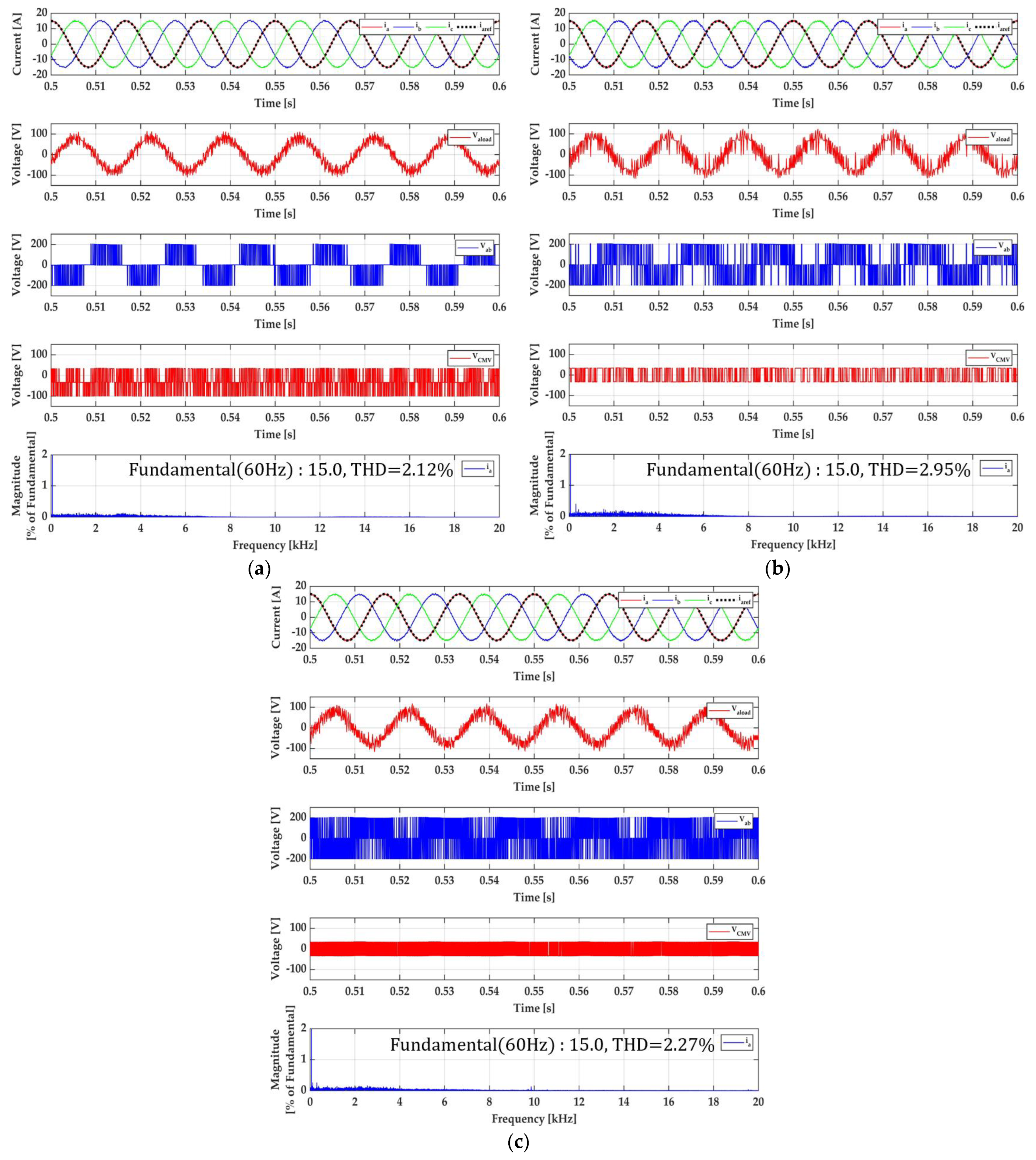
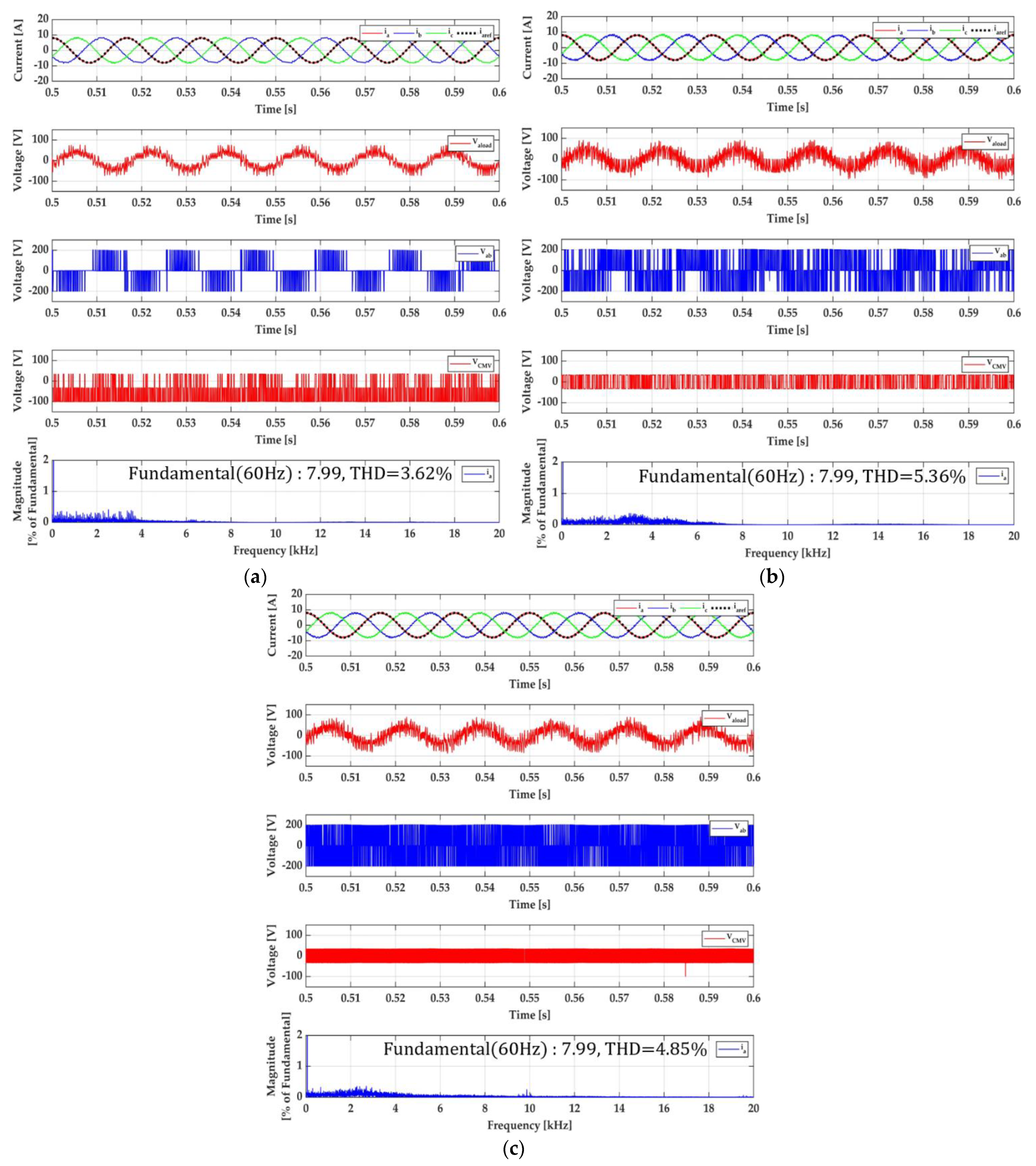
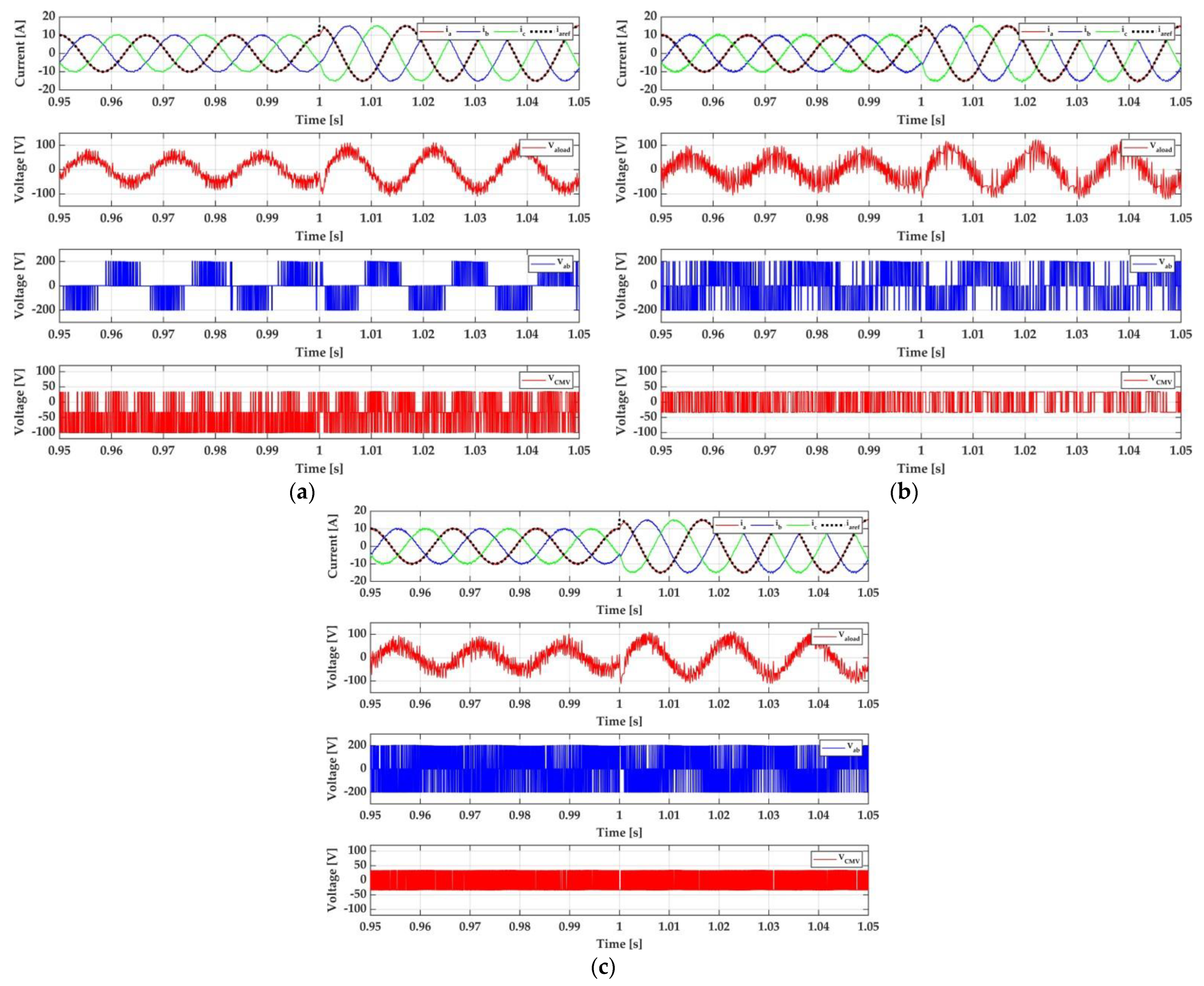
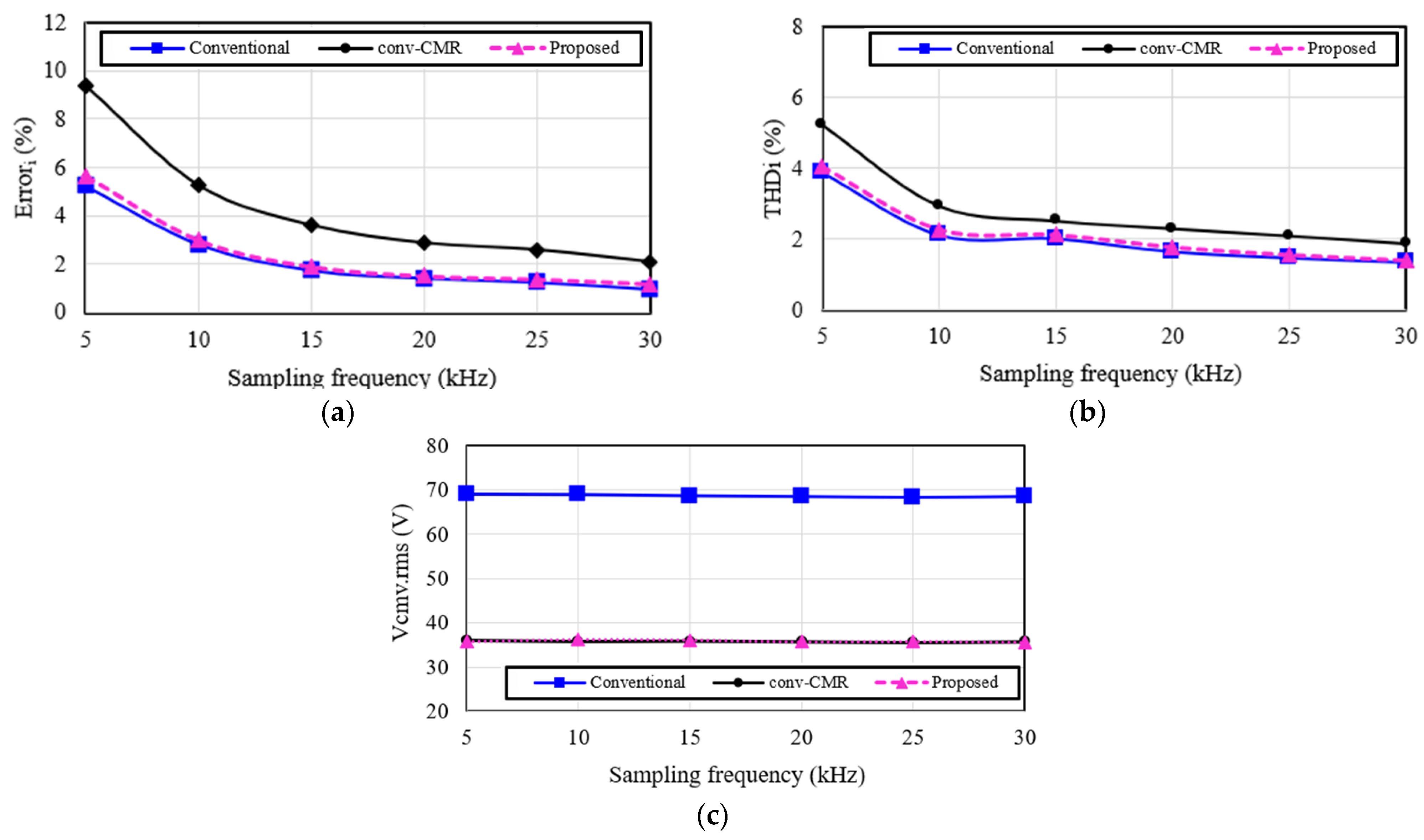
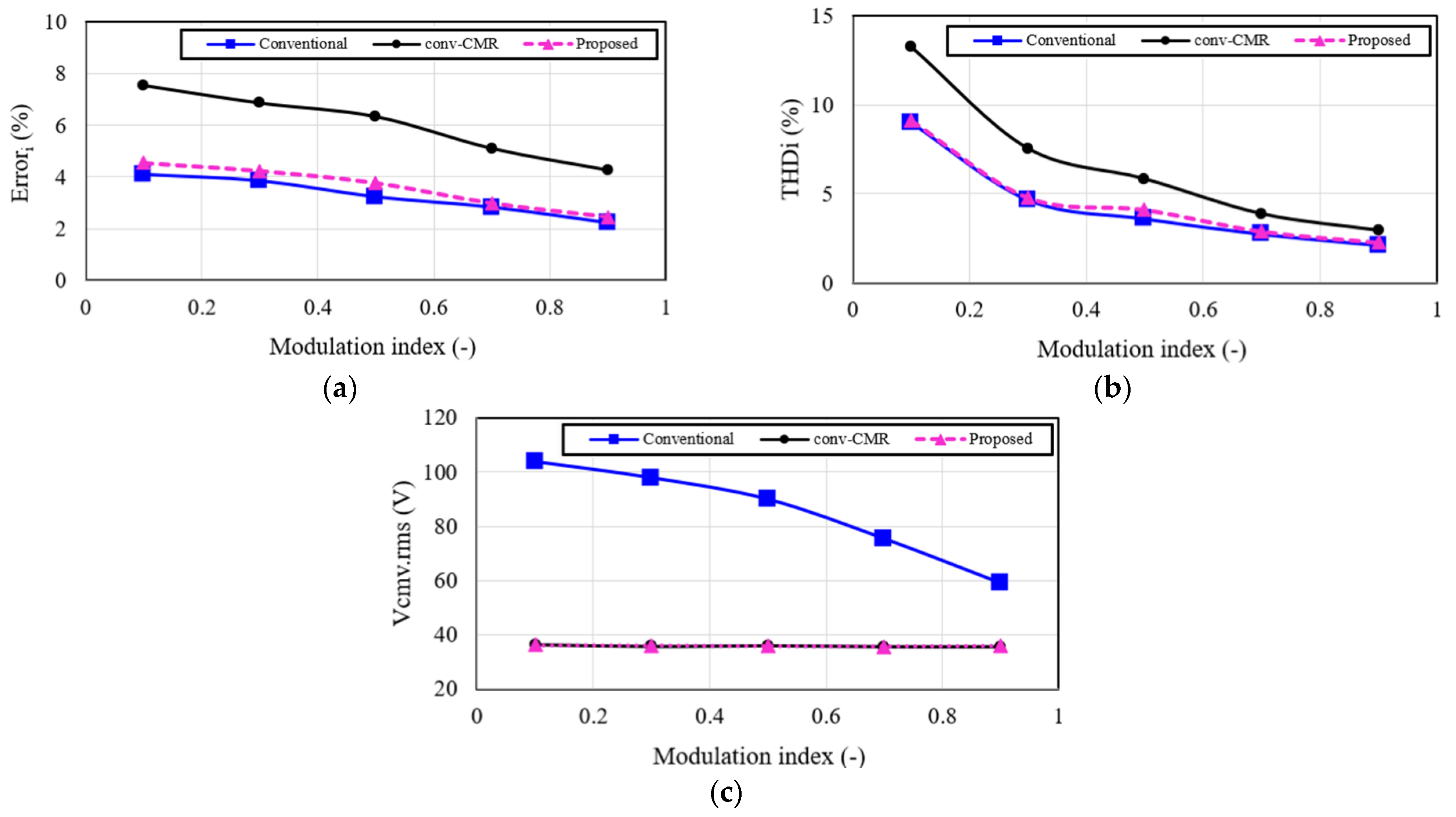
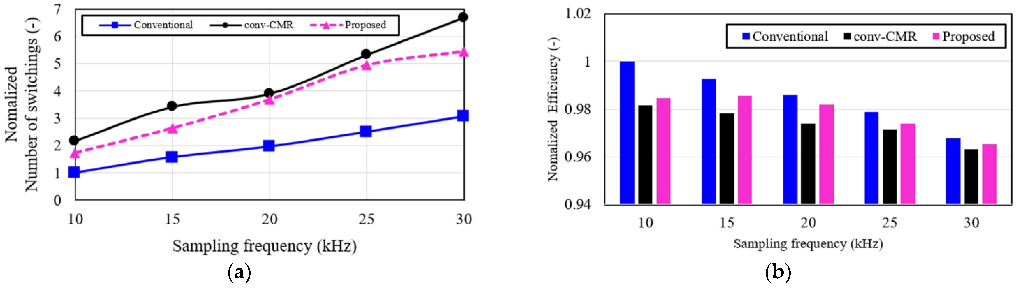
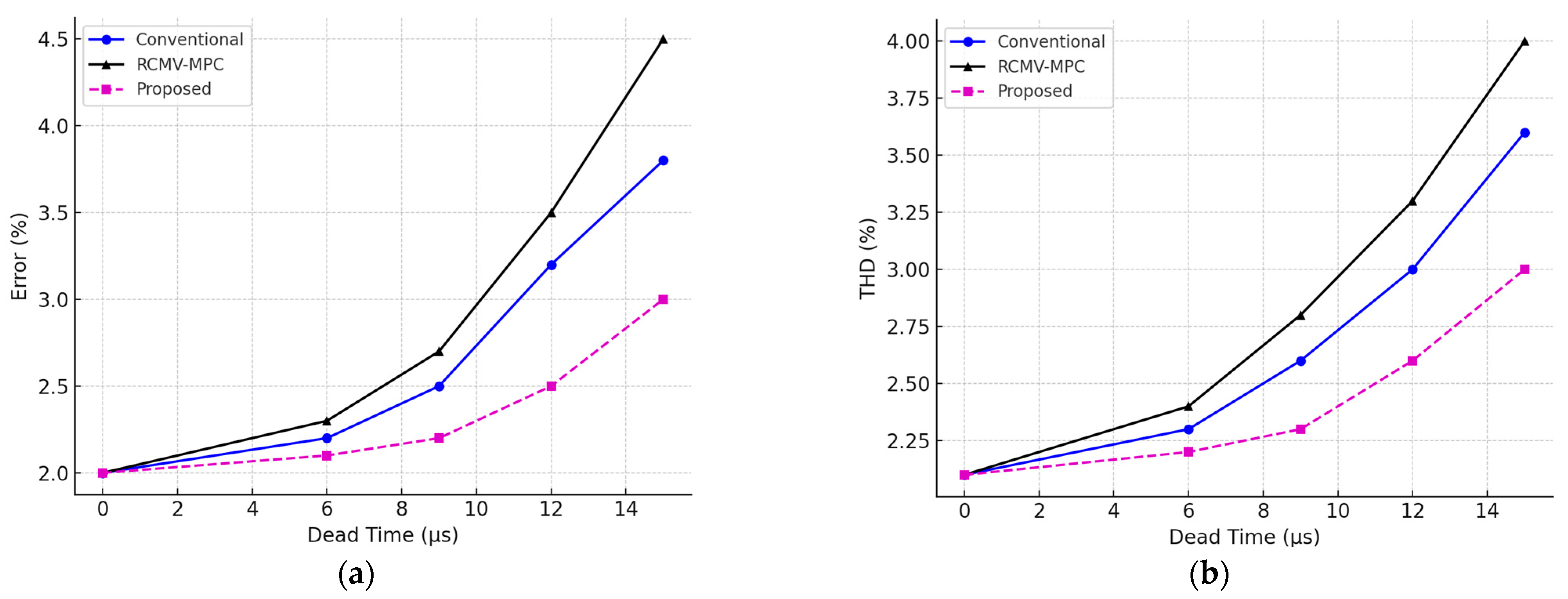
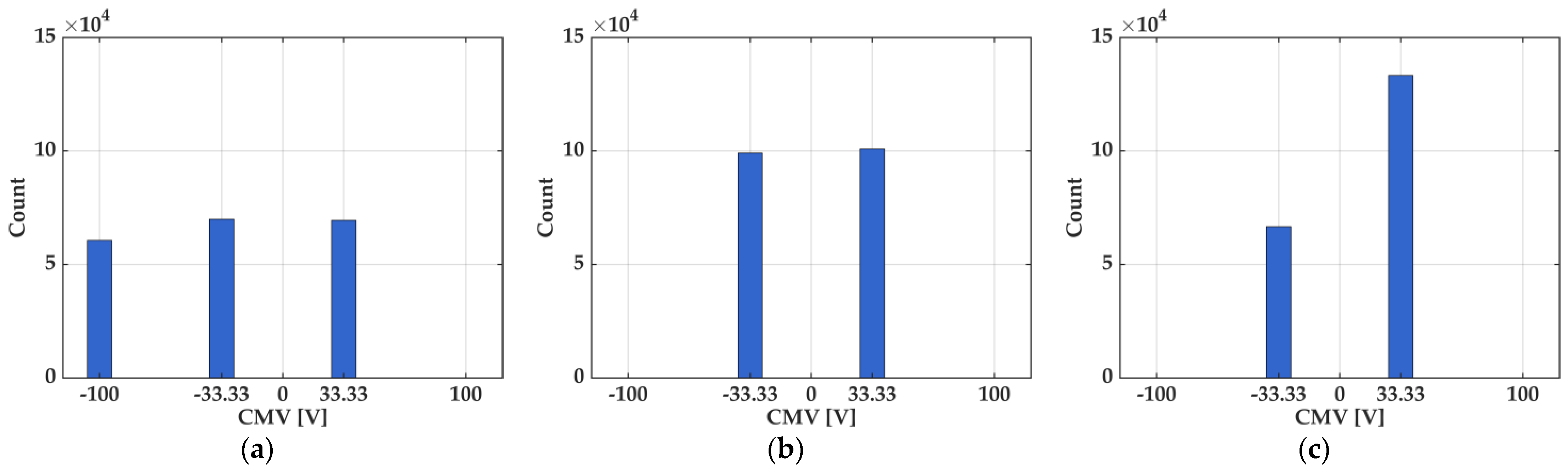
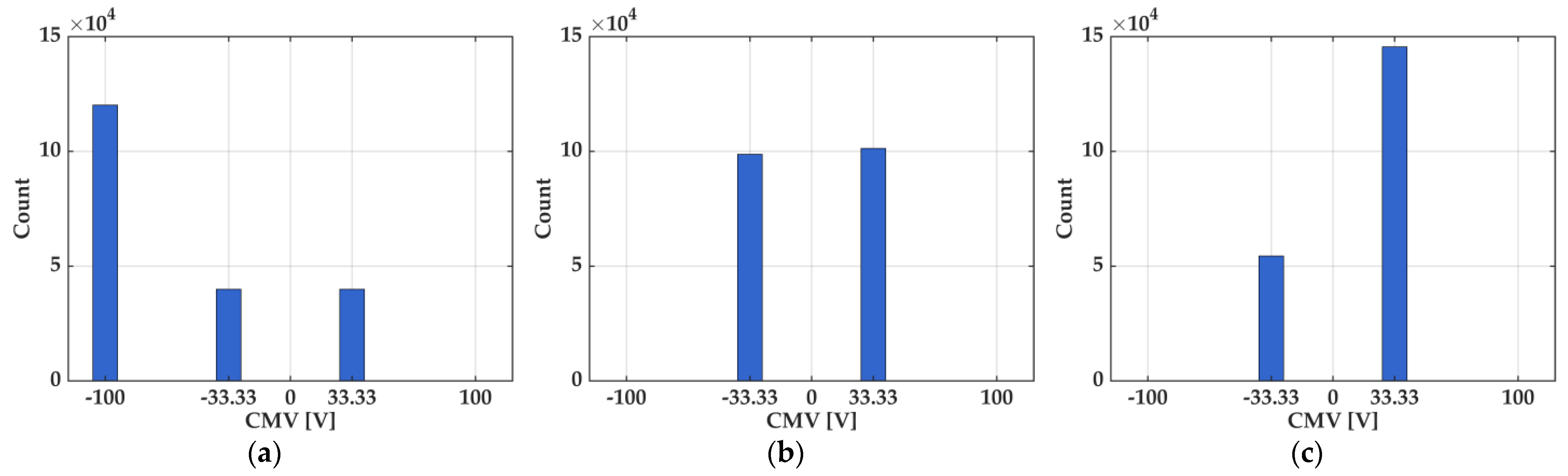
4. Simulation and Experimental Results
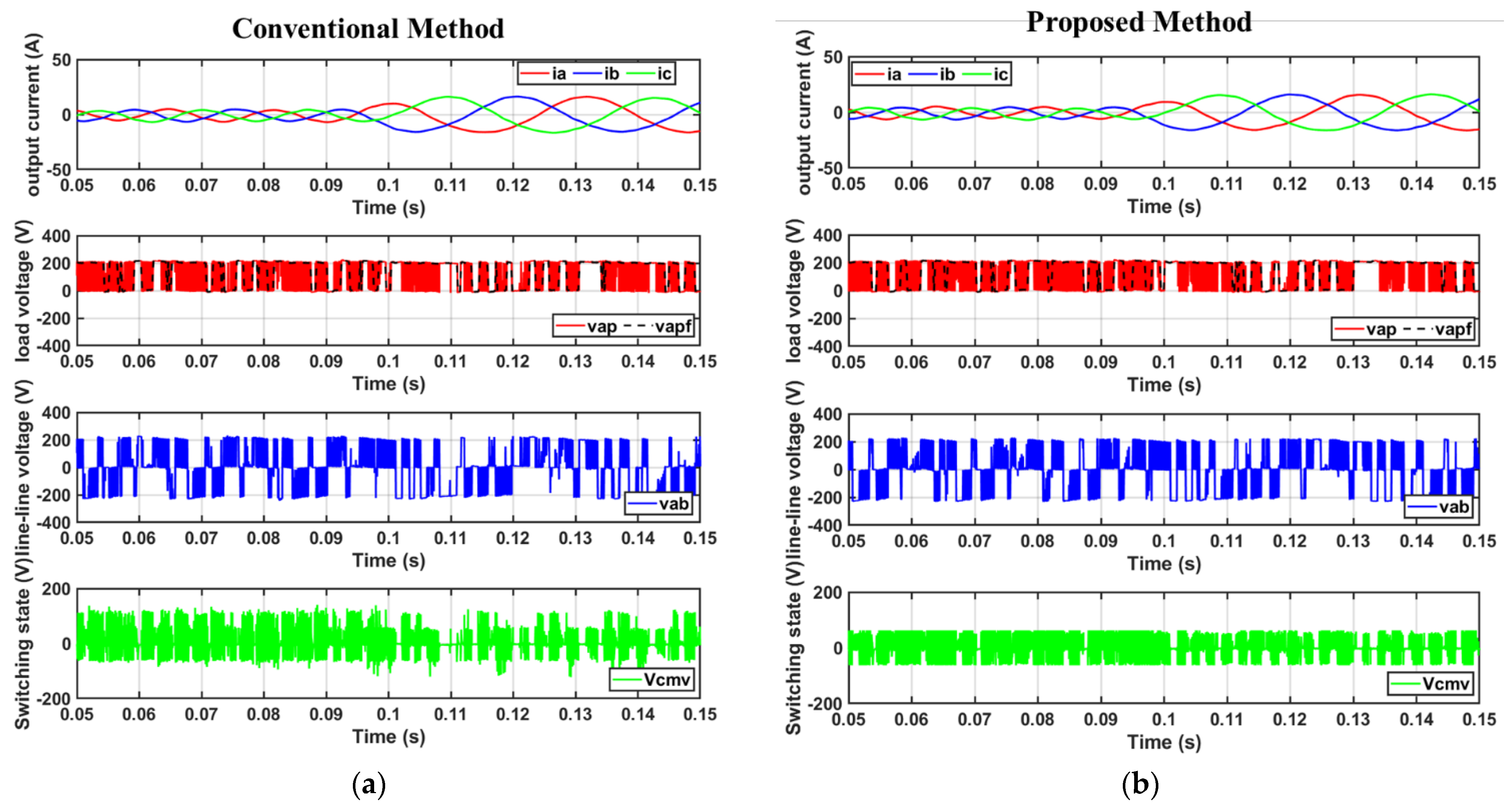
4.1. Simulation Results
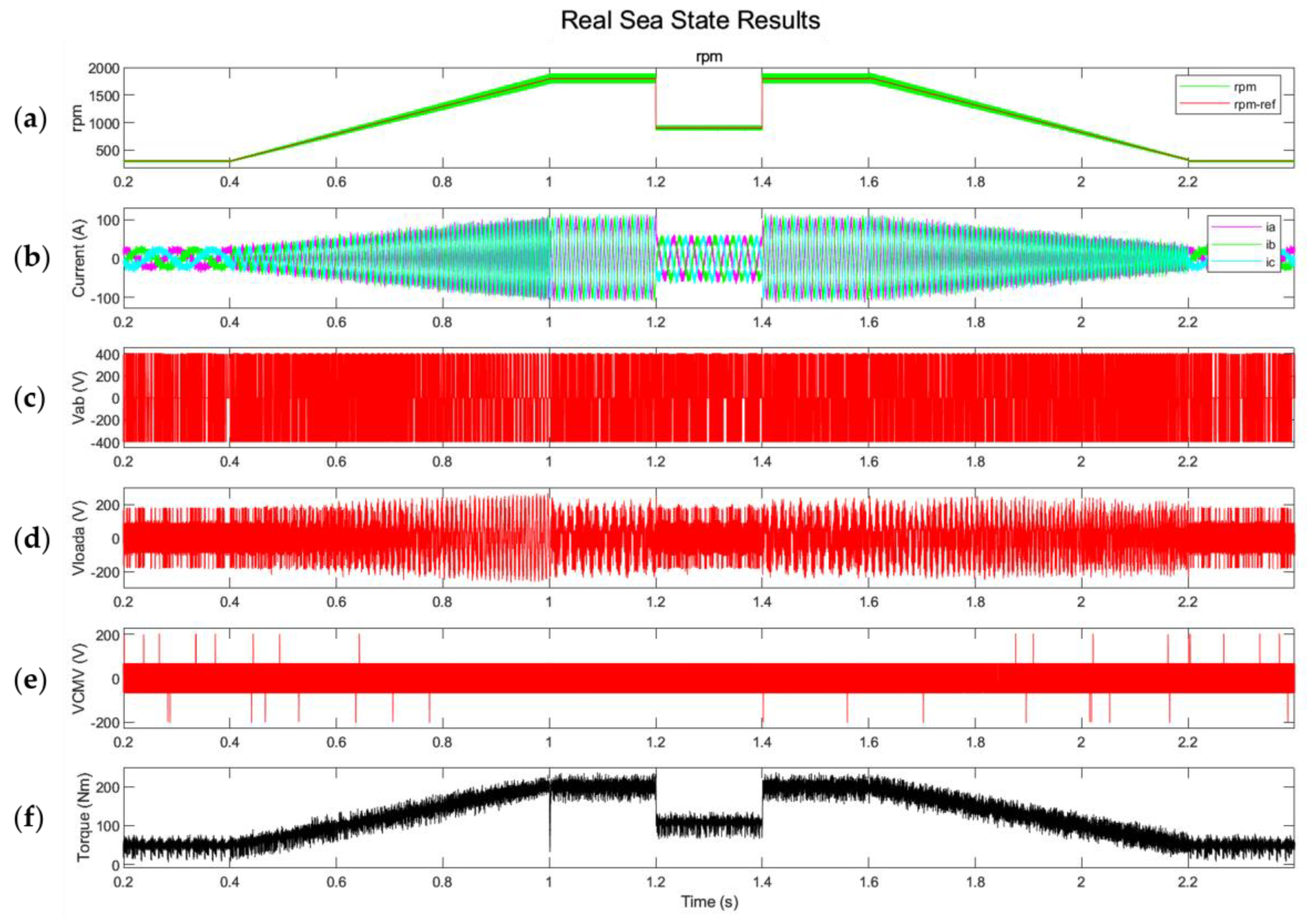
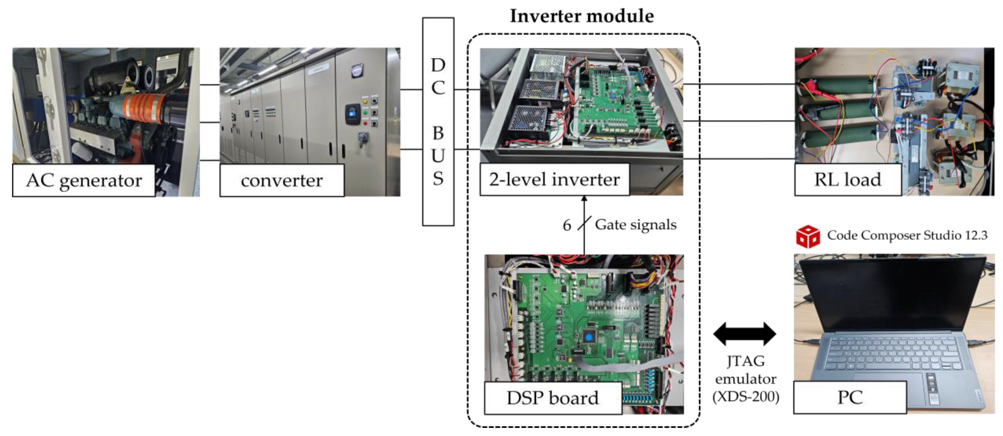
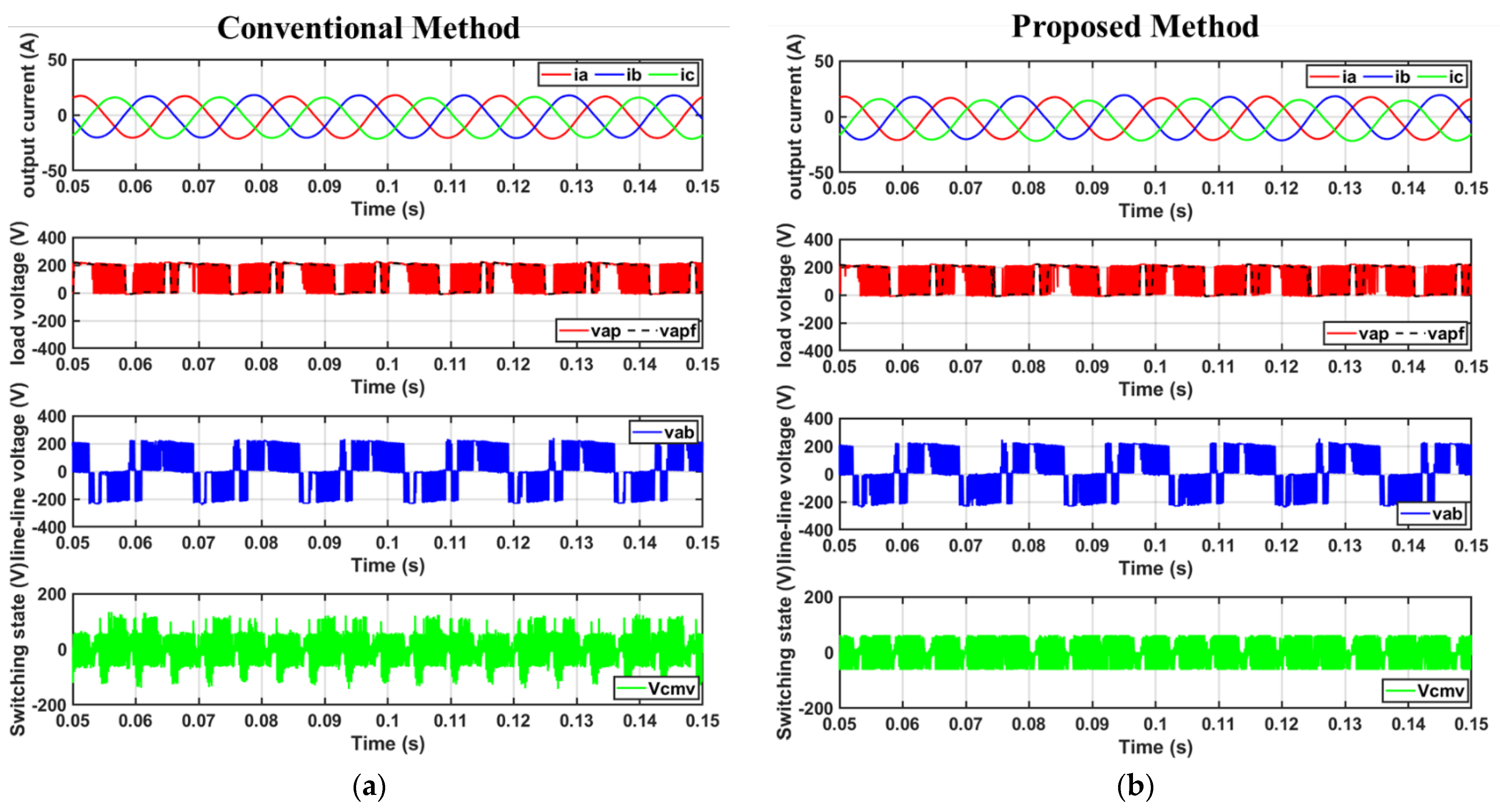
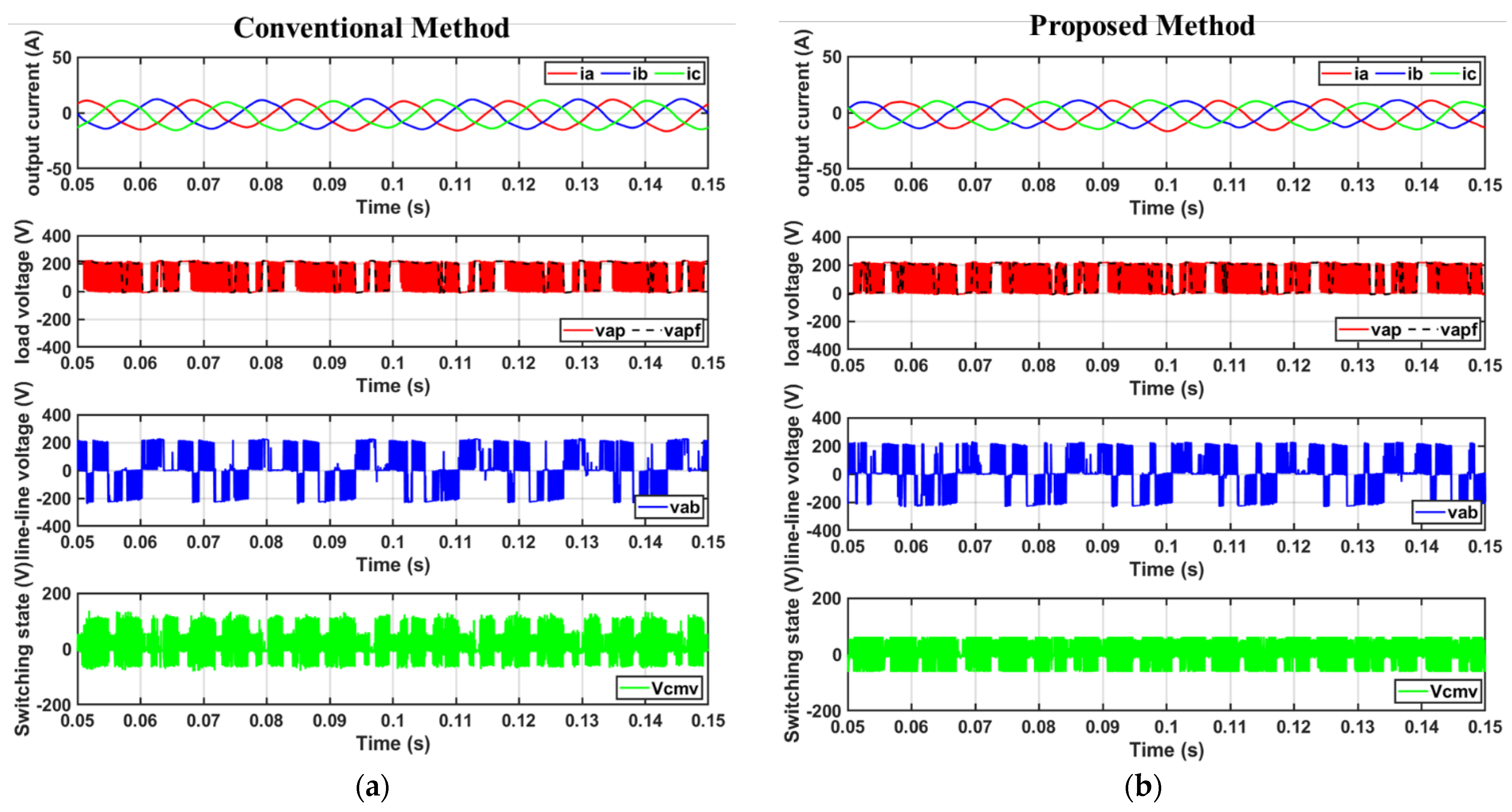
4.2. Experimental Results
5. Conclusions
- A novel zero-vector-free MPC strategy is proposed based on virtual vector synthesis using voltage sector and modulation index.
- The method achieves a 66.7% reduction in CMV and a 22.8% reduction in current THD under low modulation index conditions.
- Simulation and experimental results confirm consistent performance across steady-state, transient, and parameter-mismatched conditions.
- The average DSP execution time is reduced to 22.71 μs, providing 77.3% available computation time.
- The approach ensures low switching frequency and computational complexity by reducing candidate vectors to 2–3 per sector.
- The method is suitable for real-time implementation and can be extended to multilevel inverters and other high-reliability applications.
Author Contributions
Funding
Data Availability Statement
Conflicts of Interest
References
- Ančić, I.; Šestan, A. Influence of the required EEDI reduction factor on the CO2 emission from bulk carriers. Energy Policy 2015, 84, 107–116. [Google Scholar] [CrossRef]
- Nguyen, H.P.; Hoang, A.T.; Nizetic, S.; Nguyen, X.P.; Le, A.T.; Luong, C.N.; Chu, V.D.; Pham, V.V. The electric propulsion system as a green solution for management strategy of CO2 emission in ocean shipping: A comprehensive review. Int. Trans. Electr. Energy Syst. 2021, 31, e12580. [Google Scholar] [CrossRef]
- Liserre, M.; Sauter, T.; Hung, J.Y. Future energy systems: Integrating renewable energy sources into the smart power grid through industrial electronics. IEEE Ind. Electron. Mag. 2010, 4, 18–37. [Google Scholar] [CrossRef]
- Erdman, J.M.; Kerkman, R.J.; Schlegel, D.W.; Skibinski, G.L. Effect of pwm inverters on ac motor bearing currents and shaft voltages. IEEE Trans. Ind. Appl. 1996, 32, 250–259. [Google Scholar] [CrossRef]
- Moreira, A.F.; Lipo, T.A.; Venkataramanan, G.; Bernet, S. High-frequency modeling for cable and induction motor overvoltage studies in long cable drives. IEEE Trans. Ind. Appl. 2002, 38, 1297–1306. [Google Scholar] [CrossRef]
- De Broe, A.M.; Julian, A.L.; Lipo, T.A. Neutral-to-ground voltage minimization in a pwm-rectifier/inverter configuration. In Proceedings of the Sixth International Conference on Power Electronics and Variable Speed Drives (Conf. Publ. No. 429), Nottingham, UK, 23–25 September 1996; pp. 564–568. [Google Scholar] [CrossRef]
- Cacciato, M.; Consoli, A.; Scarcella, G.; Testa, A. Reduction of common-mode currents in pwm inverter motor drives. IEEE Trans. Ind. Appl. 1999, 35, 469–476. [Google Scholar] [CrossRef]
- Muetze, A.; Binder, A. Don’t lose your bearings. IEEE Ind. Appl. Mag. 2006, 12, 22–31. [Google Scholar] [CrossRef]
- Duran, M.J.; Riveros, J.A.; Barrero, F.; Guzman, H.; Prieto, J. Reduction of common-mode voltage in five-phase induction motor drives using predictive control techniques. IEEE Trans. Ind. Appl. 2012, 48, 2059–2067. [Google Scholar] [CrossRef]
- Chen, S.; Lipo, T.A.; Fitzgerald, D. Modeling of motor bearing currents in PWM inverter drives. IEEE Trans. Ind. Applicat. 1996, 32, 1365–1370. [Google Scholar] [CrossRef]
- Xie, Y.; Jiang, D.; Hu, F.; Liu, Z. Research on common mode EMI and its reduction for active magnetic bearings. IEEE Trans. Power Electron. 2023, 38, 4246–4250. [Google Scholar] [CrossRef]
- Wang, S.; Lee, F.C. Analysis and applications of parasitic capacitance cancellation techniques for EMI suppression. IEEE Trans. Ind. Electron. 2010, 57, 3109–3117. [Google Scholar] [CrossRef]
- Zhong, E.; Lipo, T.A. Improvements in EMC performance of inverter-fed motor drives. IEEE Trans. Ind. Appl. 1995, 31, 1247–1256. [Google Scholar] [CrossRef]
- Tian, K.; Wang, J.; Wu, B.; Cheng, Z.; Zargari, N.R. A virtual space vector modulation technique for the reduction of common-mode voltages in both magnitude and third-order component. IEEE Trans. Power Electron. 2016, 31, 839–848. [Google Scholar] [CrossRef]
- Cavalcanti, M.C.; de Oliveira, K.C.; Neves, F.A.S.; Azevedo, G.M.S.; Camboim, F.C. Modulation techniques to eliminate leakage currents in transformerless three-phase photovoltaic systems. IEEE Trans. Ind. Electron. 2010, 57, 1360–1368. [Google Scholar] [CrossRef]
- Kim, H.-J.; Lee, H.D.; Sul, S.-K. A new PWM strategy for common-mode voltage reduction in neutral-point-clamped inverter-fed AC motor drives. IEEE Trans. Ind. Appl. 2001, 37, 1840–1845. [Google Scholar] [CrossRef]
- Lakshminarayanan, S.; Mondal, G.; Tekwani, P.N.; Mohapatra, K.K.; Gopakumar, K. Twelve-sided polygonal voltage space vector based multilevel inverter for an induction motor drive with common-mode voltage elimination. IEEE Trans. Ind. Electron. 2007, 54, 2761–2768. [Google Scholar] [CrossRef]
- Lai, Y.S.; Shyu, F.S. Optimal common-mode voltage reduction PWM technique for inverter control with consideration of the dead-time effects—Part I: Basic development. IEEE Trans. Ind. Appl. 2004, 40, 1605–1612. [Google Scholar] [CrossRef]
- Kimball, J.W.; Zawodniok, M. Reducing common-mode voltage in three-phase sine-triangle PWM with interleaved carriers. IEEE Trans. Power Electron. 2011, 26, 2229–2236. [Google Scholar] [CrossRef]
- Chen, J.; Jiang, D.; Li, Q. Attenuation of conducted EMI for three-level inverters through PWM. CPSS Trans. Power Electron. Appl. 2018, 3, 134–145. [Google Scholar] [CrossRef]
- Hoseini, S.K.; Adabi, J.; Sheikholeslami, A. Predictive modulation schemes to reduce common-mode voltage in three-phase inverters-fed AC drive systems. IET Power Electron. 2014, 7, 840–849. [Google Scholar] [CrossRef]
- Kwak, S.; Mun, S.K. Model predictive control methods to reduce common-mode voltage for three-phase voltage source inverters. IEEE Trans. Power Electron. 2015, 30, 5019–5035. [Google Scholar] [CrossRef]
- Kwak, S.; Mun, S. Common-mode voltage mitigation with a predictive control method considering dead time effects of three-phase voltage source inverters. IET Power Electron. 2015, 8, 1690–1700. [Google Scholar] [CrossRef]
- Guo, L.; Jin, N.; Gan, C.; Xu, L.; Wang, Q. An improved model predictive control strategy to reduce common-mode voltage for two-level voltage source inverters considering dead-time effects. IEEE Trans. Ind. Electron. 2019, 66, 3561–3572. [Google Scholar] [CrossRef]
- Li, X.; Xie, M.; Ji, M.; Yang, J.; Wu, X.; Shen, G. Restraint of common-mode voltage for PMSM-inverter systems with current ripple constraint based on voltage-vector MPC. IEEE J. Emerg. Sel. Top. Ind. Electron. 2023, 4, 688–697. [Google Scholar] [CrossRef]
- Tang, X.; Yuan, X.; Niu, S.; Chau, K.T. High-efficient multivector model predictive control with common-mode voltage suppression. IEEE J. Emerg. Sel. Top. Power Electron. 2024, 12, 2674–2685. [Google Scholar] [CrossRef]
- Monfared, K.K.; Iman-Eini, H.; Neyshabouri, Y.; Liserre, M. Model predictive control with reduced common-mode voltage based on optimal switching sequences for nested neutral point clamped inverter. IEEE Trans. Ind. Electron. 2024, 71, 27–38. [Google Scholar] [CrossRef]
- Bebboukha, A.; Meneceur, R.; Chouaib, L.; Anees, M.A.; Elsanabary, A.; Mekhilef, S.; Bakeer, A.; Harbi, I.; Zaitsev, I.; Bajaj, M. Finite control set model predictive current control for three-phase grid-connected inverter with common mode voltage suppression. Sci. Rep. 2024, 14, 19832. [Google Scholar] [CrossRef] [PubMed]
- Cortes, P.; Rodriguez, J.; Silva, C.; Flores, A. Delay compensation in model predictive current control of a three-phase inverter. IEEE Trans. Ind. Electron. 2012, 59, 1323–1325. [Google Scholar] [CrossRef]
- Xia, C.; Liu, T.; Shi, T.; Song, Z. A simplified finite-control-set model-predictive control for power converters. IEEE Trans. Ind. Inform. 2014, 10, 991–1002. [Google Scholar] [CrossRef]


| Ref. | Main Principle | Advantages | Limitations |
|---|---|---|---|
| [21] | Predictive switching using only non-zero vectors | Simple implementation; effective CMV reduction | Increases current ripple at low speed/light load |
| [22] | Synthesizing virtual reference using two active vectors | Improved voltage tracking | Higher switching loss and ripple under low speed |
| [23] | Replace zero vectors with reverse ones; exclude opposite vectors | CMV reduction with dead-time compensation | Limited vector options; Increased THD and ripple |
| [24] | Divide vector plane into sectors; allow limited asymmetric vectors | Balanced CMV suppression and control flexibility | Implementation complexity |
| [25] | Select two vectors per cycle: one active, one from zero region | CMV suppression with ripple constraint | Computational complexity in selection logic |
| [26] | Use four active vectors to emulate zero vector effect | High efficiency and CMV suppression | Increased switching complexity |
| [27] | Apply optimal MPC switching to Nested NPC inverter | Effective for multilevel topologies; strong CMV reduction | High computational burden; topology-specific |
| [28] | Add CMV cost term for grid-connected VSI | Simultaneous CMV suppression and accurate current tracking | High processing demand; limited to grid-tied VSI systems |
| List of Abbreviation | ||
| Abbreviation | Definition | |
| CMV | Common-Mode Voltage | |
| PWM | Pulse Width Modulation | |
| THD | Total Harmonic Distortion | |
| MPC | Model Predictive Control | |
| FCS-MPC | Finite Control Set Model Predictive Control | |
| RCMV-MPC | Reduced Common-Mode Voltage Model Predictive Control | |
| VSI | Voltage Source Inverter | |
| MI | Modulation Index | |
| List of Nomenclature | ||
| Symbol | Definition | Unit |
| Load resistance | Ω | |
| Load inductance | H | |
| Sampling period | s | |
| -axis components of the applied voltage vector at time k | V | |
| Reference voltage vector at time k | V | |
| Load current vector at time k | A | |
| Reference load current at time k | A | |
| Back electromotive force | V | |
| DC-link voltage | V | |
| Root mean square value of common-mode voltage | V | |
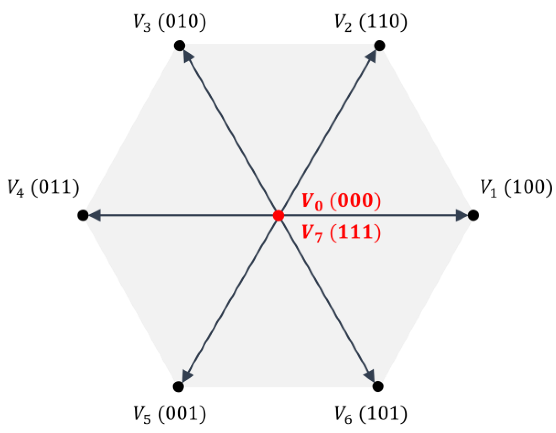
| Vectors | Switching States | Common-Mode Voltage | ||
|---|---|---|---|---|
| 0 | 0 | 0 | ||
| 1 | 0 | 0 | ||
| 1 | 1 | 0 | ||
| 0 | 1 | 0 | ||
| 0 | 1 | 1 | ||
| 0 | 0 | 1 | ||
| 1 | 0 | 1 | ||
| 1 | 1 | 1 | ||
| Sector | 0.5) | 0.5) |
|---|---|---|
| 1-1 | V5-V3-V1 | V1-V5-V3 |
| 1-2 | V4-V2-V6 | V2-V6-V4 |
| 2-1 | V6-V4-V2 | V2-V6-V4 |
| 2-2 | V5-V3-V1 | V3-V1-V5 |
| 3-1 | V1-V5-V3 | V3-V1-V5 |
| 3-2 | V6-V4-V2 | V4-V2-V6 |
| 4-1 | V2-V6-V4 | V4-V2-V6 |
| 4-2 | V1-V5-V3 | V5-V3-V1 |
| 5-1 | V3-V1-V5 | V5-V3-V1 |
| 5-2 | V2-V6-V4 | V6-V4-V2 |
| 6-1 | V4-V2-V6 | V6-V4-V2 |
| 6-2 | V3-V1-V5 | V1-V5-V3 |
| Parameters | Values |
|---|---|
| (DC voltage) | 200 V |
| (Load resistance) | 1.233 Ω |
| (Load inductance) | 9.873 mH |
| (DC capacitance) | 4400 µF |
| (Load current) | 15 A |
| Parameters | Values |
|---|---|
| Rated power | 50 kW |
| Rated voltage | 440 V |
| Rated frequency | 60 Hz |
| Number of poles | 4 |
| Rated speed | 1780~1800 rpm |
| Rated current | 95~110 A |
| Power factor (cosφ) | 0.87~0.93 |
| Efficiency | Over 93% |
| Motor torque | 265 Nm |
| Moment of inertia (J) | 0.2~0.4 kg·m2 |
| Stator resistance (Rs) | 0.5 Ω |
| Leakage inductance (Ls) | 5~15 mH |
| Rotor resistance (Rr) | 0.2~0.4 Ω |
| Magnetizing Inductance (Lm) | 100~200 mH |
| Parameters | Values |
|---|---|
| (DC voltage) | 200 V |
| (Load resistance) | 1.0 Ω |
| (Load inductance) | 8.9 mH |
| (DC capacitance) | 4400 μF |
| Control Method | DSP Execution Time (μs) | Usage Rate (%) | Available Computational Time (%) |
|---|---|---|---|
| Conventional MPC | 30.88 | 30.88 | 69.12 |
| RCMV-MPC | 28.21 | 28.21 | 71.79 |
| Proposed MPC | 22.71 | 22.71 | 77.29 |
| Metric | Conventional MPC | RCMV-MPC | Proposed MPC | Improvement (%) |
|---|---|---|---|---|
| CMV RMS (V) | 100.0 | 33.33 | 35.00 | −65% (↓); CM suppression |
| THD (%) | 2.12 | 2.95 | 2.27 | −6.6% (↓) |
| Current error (MI = 0.45) | Minimum (Ref.) | +59.7% ↑ | +20.9% ↑ | Less degradation (vs. RCMV) |
| DSP Execution Time (s) | 30.88 | 28.21 | 22.71 | −26.5% (↓) |
| Category | Tang et al. (2024) [26] | Proposed Method |
|---|---|---|
| Control structure | Combination of four active vectors to emulate zero vector effect | Predefined virtual vector synthesis |
| CMV reduction | ~45% reduction | ~53.6% reduction |
| THD improvement | ~15–20% reduction | ~22.8% reduction |
| Computational complexity | High due to combinatorial vector search | Low due to sector-based, limited vector set |
| Real-time applicability | Not validated; simulation only | DSP-verified (22.7 μs execution time) |
| Target application | EV drive and general inverter systems | Marine electric propulsion system |
Disclaimer/Publisher’s Note: The statements, opinions and data contained in all publications are solely those of the individual author(s) and contributor(s) and not of MDPI and/or the editor(s). MDPI and/or the editor(s) disclaim responsibility for any injury to people or property resulting from any ideas, methods, instructions or products referred to in the content. |
© 2025 by the authors. Licensee MDPI, Basel, Switzerland. This article is an open access article distributed under the terms and conditions of the Creative Commons Attribution (CC BY) license (https://creativecommons.org/licenses/by/4.0/).
Share and Cite
Song, S.-w.; Roh, C. Zero-Vector-Free MPC with Virtual Vector Synthesis for CMV Suppression in Electric Propulsion Systems. J. Mar. Sci. Eng. 2025, 13, 1010. https://doi.org/10.3390/jmse13061010
Song S-w, Roh C. Zero-Vector-Free MPC with Virtual Vector Synthesis for CMV Suppression in Electric Propulsion Systems. Journal of Marine Science and Engineering. 2025; 13(6):1010. https://doi.org/10.3390/jmse13061010
Chicago/Turabian StyleSong, Sung-woo, and Chan Roh. 2025. "Zero-Vector-Free MPC with Virtual Vector Synthesis for CMV Suppression in Electric Propulsion Systems" Journal of Marine Science and Engineering 13, no. 6: 1010. https://doi.org/10.3390/jmse13061010
APA StyleSong, S.-w., & Roh, C. (2025). Zero-Vector-Free MPC with Virtual Vector Synthesis for CMV Suppression in Electric Propulsion Systems. Journal of Marine Science and Engineering, 13(6), 1010. https://doi.org/10.3390/jmse13061010