Short-Term Prediction of Ship Heave Motion Using a PSO-Optimized CNN-LSTM Model

Abstract

When ships conduct offshore operations in the ocean, they are subject to disturbances from natural factors such as sea breezes and waves. These disturbances lead to movements detrimental to the ship’s stability, especially heave movement in the vertical direction, which profoundly impacts the safety of shipboard facilities and staff. To counter this, the active wave compensation device is widely used on ships to maintain the stability of the working environment. However, the system’s efficiency and accuracy are compromised by the significant delay incurred while obtaining real-time motion signals and driving the actuator for motion compensation. To solve the time delay problem of shipborne wave compensation equipment in motion compensation under complex sea conditions, it is necessary to improve the ship heave motion prediction accuracy in an active wave compensation system. This paper presents a prediction method of ship heave motion based on the particle swarm optimization (PSO) and convolutional neural network–long short-term memory (CNN-LSTM) hybrid prediction model. The paper begins by establishing the ship heave motion model based on the P–M spectrum and slice theory, simulating the ship heave motion curve under different sea conditions on MATLAB. This simulation provides crucial data for the subsequent prediction model. The paper then delves into the realization method of ship heave motion based on PSO-CNN-LSTM, where the convolutional neural network (CNN) is used to extract the features of the input signal, thereby enhancing the multi-source feature fusion ability of the LSTM neural network model. The PSO algorithm is then employed to optimize the network structure and hyperparameters of the convolutional neural network. The experiments demonstrate that the proposed PSO-CNN-LSTM hybrid model effectively addresses the problem of predicting drift and boasts significantly higher prediction accuracy, making it suitable for predicting the short-term heave motion of ships. The data show that the optimized root mean square error (RMSE) value under level 5 sea conditions is 0.01265 compared to 0.01673 before optimization, and the optimized RMSE value under level 6 sea conditions is 0.01140 compared to 0.01479 before optimization, which demonstrates that the error between the predicted value and the actual value of the model decreases. This improved accuracy provides reassurance in the model’s predictive capabilities and lays the foundation for improving the accuracy of the motion compensation system in the future.

1. Introduction

With the vigorous development of the global shipping industry and the rapid development of science and technology, countries around the world began to pay attention to the development of marine activities such as the exploration of marine resources, marine biological research, offshore platform construction, and ocean-going operations of ships [1,2]. However, the marine environment is a complex and challenging one. Maintaining a stable working environment on the sea as on land is not easy. Under the influence of waves and sea winds, offshore ships may produce a variety of complex motions, including six degrees of freedom motions such as roll, pitch, yaw, sway, surge, and heave, which will greatly affect the stability of shipborne facilities and the safety of staff. The heave motion in the vertical direction has the most significant impact on the safety of shipborne facilities and staff [3,4].

Therefore, researchers worldwide began to design and study the wave compensation system [5,6] to reduce the impact of ship coupling motion. The wave compensation system is divided into two main categories: a passive wave compensation system and an active wave compensation system. The compensation range and accuracy of the passive wave compensation system are not easy to control, so researchers have conducted in-depth research [7,8]. However, when the active wave compensation system compensates the motion of shipborne equipment, it will experience a complex process of the sensor capturing the motion signal, sensor transmitting the motion signal to the controller, the controller calculating the motion compensation amount and transmitting it to the actuator, and the actuator implementing the motion in the opposite direction to realize the compensation. After this process, the coupled motion of the ship caused by ocean waves will change again, so there will be a severe time delay, which will affect the efficiency and accuracy of wave compensation, the stability of shipborne facilities, and the safety of staff [9]. Therefore, it is necessary to collect the ship’s past motion and predict the ship’s motion in advance by adding a prediction module to calculate the motion compensation for the controller.

With the rapid development of computer technology, machine learning and deep learning with high generalization and self-adaptability are widely used in ship motion prediction [10,11]. Z. Chen and L. Huang et al., introduced a cycle reservoir with regular jumps (CRJ) modeling method to address the ship motion prediction issue [11,12]. Y. Wei et al. studied the non-dominated sorting genetic algorithm-II (NSGA-II) algorithm, which was adapted for feature selection of the original multi-factor data to filter out the feature factors that are useful for ship motion prediction [13]. A linear regression model is mainly used to predict the ship motion signal in machine learning; however, linear models often fail to capture the nonlinear and dynamic characteristics of complex sea conditions, leading to inaccurate predictions, especially in processing data of complex sea conditions and complex ship motion [14].

Deep learning represented by neural networks has strong modeling ability and feature-extraction ability for nonlinear data, and it can process a large amount of complex data in parallel [15]. The ship motion data are nonlinear and unstable, and the ship motion data are long-time series data. Therefore, the LSTM that can capture the long-term dependence of time series signals is selected for prediction [16], and the gating principle is added to avoid the gradient explosion problem and enhance the stability of the prediction model. For the data of the ship’s heave motion, firstly, the CNN neural network is used to extract the characteristics of the ship’s speed information and position information, and the corresponding time dimension is used as the time series of the data [17]. The extracted features are input into the LSTM neural network for training. At the same time, the ship’s spatiotemporal and time series information are considered to predict the short-term ship motion signal, which helps the wave compensation mechanism realize pre-compensation and reduce the time delay phenomenon.

The main contributions of this paper are as follows:

(1)

A hybrid PSO-CNN-LSTM prediction model is proposed to improve the prediction accuracy of nonlinear and unsteady ship heave motion, laying the foundation for developing an active wave compensation control system;

(2)

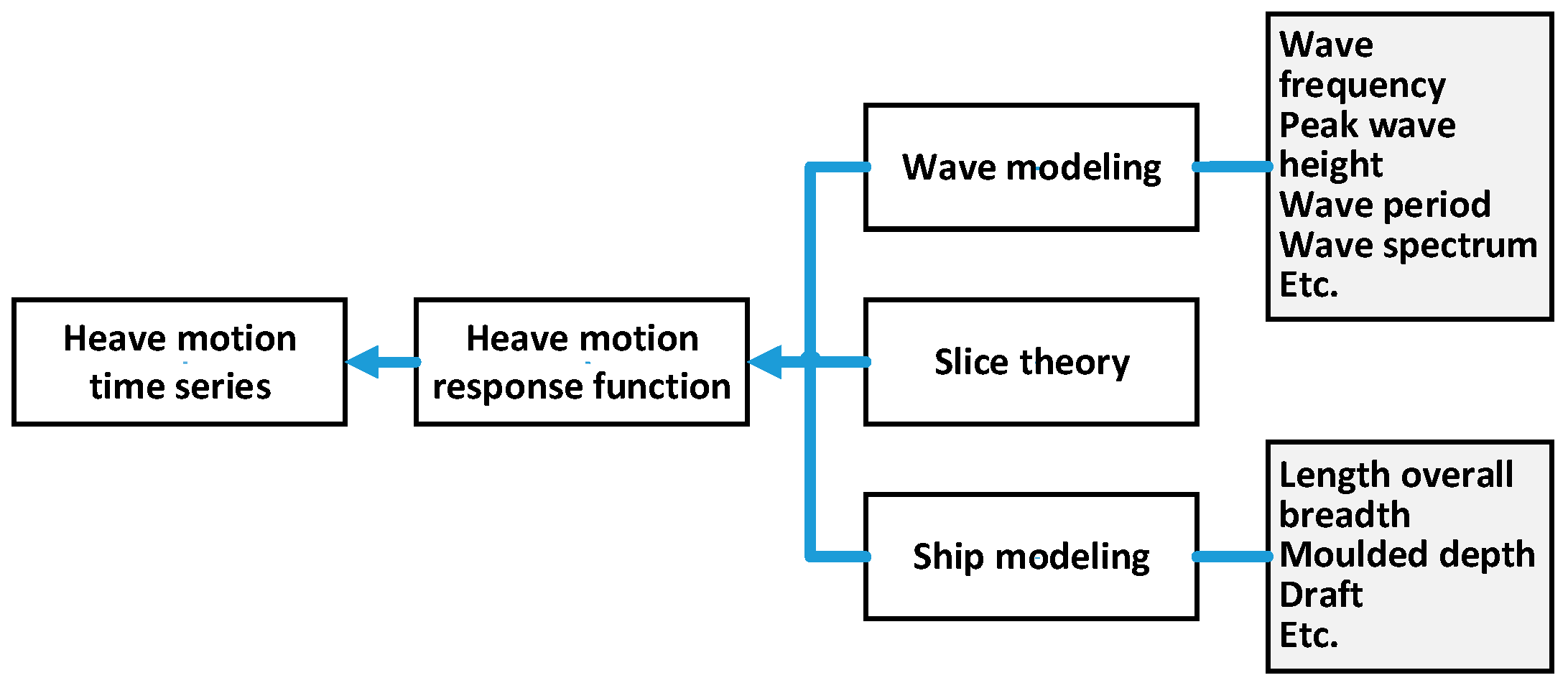
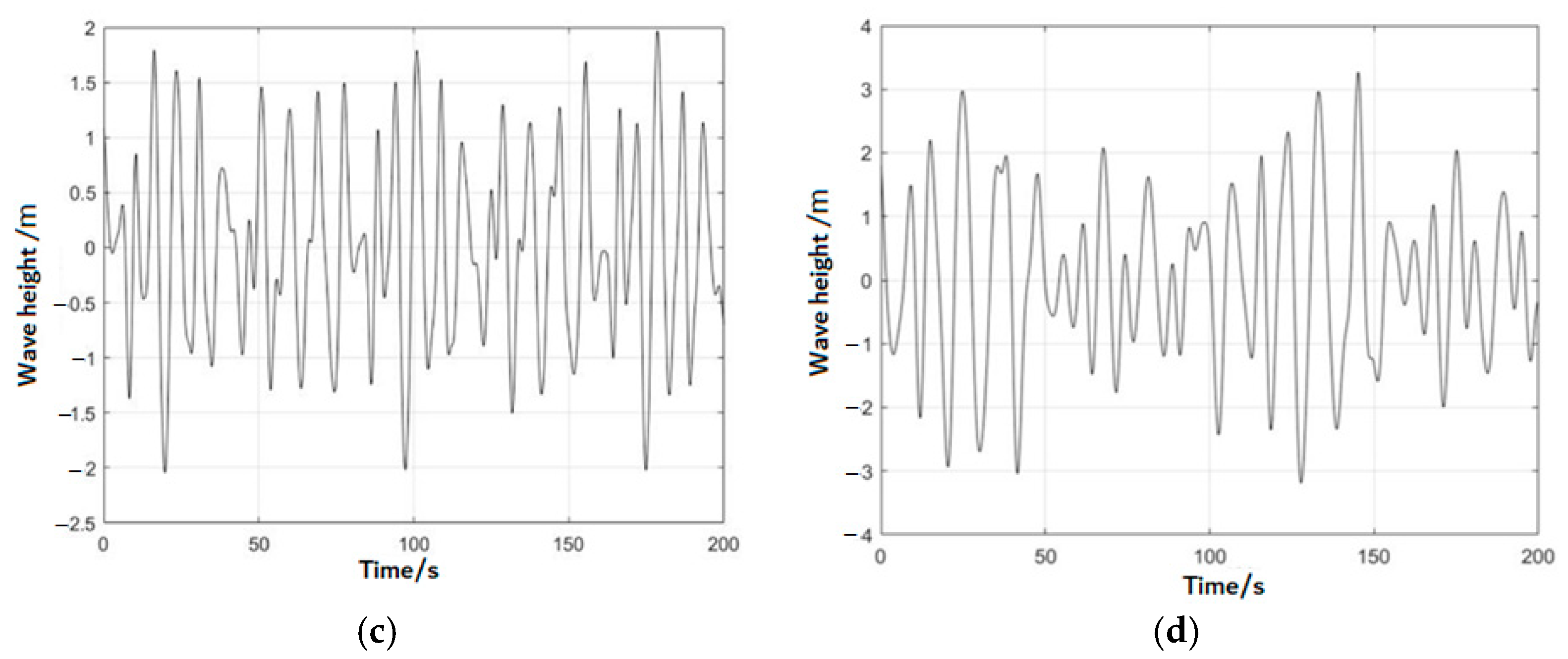
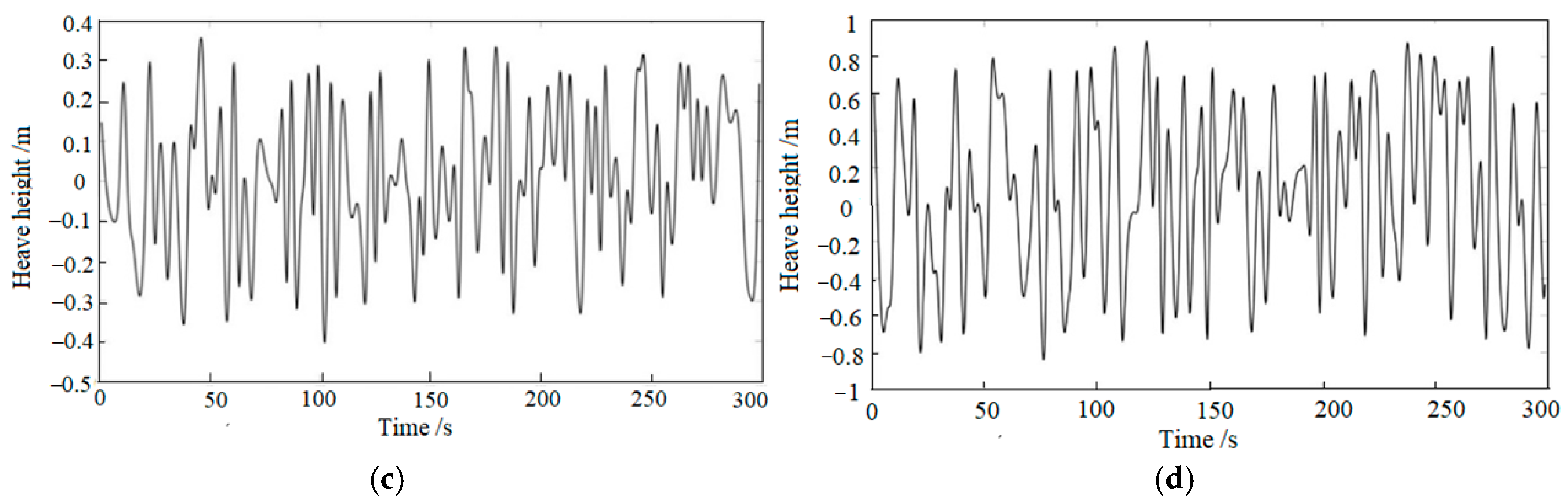
The wave model based on the P–M spectrum and the ship model based on slice theory are constructed, and the ship heave motion simulation under different sea conditions is carried out. The simulation signal is used as the input data of the PSO-CNN-LSTM prediction model;

(3)

The PSO algorithm optimizes the parameters of the CNN, and a hybrid PSO-CNN-LSTM neural network is constructed. The prediction accuracy and stability of the hybrid neural network model are verified by simulation.

The rest of this paper is organized as follows: In Section 2, the methods of wave modeling and ship heave motion modeling are proposed, and the heave motion curves of the “Yuming” ship under different sea conditions are simulated on MATLAB R2023a. The simulated heave motion signal is used as the input data for the prediction. In Section 3, the operation mechanisms of the CNN-LSTM prediction model and the hybrid PSO-CNN-LSTM prediction model are described, and the models’ prediction performances under different working conditions are verified and analyzed by simulation data. Finally, conclusions are drawn in Section 4

2. Data Generation

2.1. Modeling of Ship Heave Motion

Ships operating at sea will produce six degrees of freedom coupling motion due to the influence of waves, but now ships are equipped with anti-rolling devices to reduce the impact of pitch, yaw, and roll. In actual marine operations, the motion in the heave direction is the most important one [4], so it is necessary to analyze and study the ship’s motion in the heave direction. In this paper, the wave motion model is established according to the P–M spectrum [18,19], and then the ship model, called “Yuming”, of Shanghai Maritime University is built according to the slice theory [20,21]. Finally, the motion equation in the heave direction of the ship motion is derived according to the mechanical effect of the wave on the ship, and the response function in the heave direction is calculated according to the slice principle. As shown in Figure 1, it is the flow chart of ship heave motion modeling.

(1)

Wave Modeling

Ocean waves are low-frequency, random, and nonlinear, so no fixed formula model exists for ocean waves. However, the structure of wave motion response is linear so that the wave can be regarded as the superposition of several waves. Therefore, based on the wave spectrum, the wave can be regarded as the superposition of infinite harmonics according to the random wave theory, forming an extended crest wave model [22,23]. In practical application, the waves corresponding to the first-order sea state and the second-order sea state are small, and the impact on offshore structures is limited, so the first-order impact is rarely considered. However, in the current structural design standards, when the sea state is only level 6 or above, generally for safety reasons, the ship will stop operation. Therefore, this paper mainly deals with sea state levels 3 to 5 [24].

Table 1. Wave parameters.

Sea States	Significant Wave Height (h1/3/m)	Sea-Breeze Speed (m/s)	Wave Period (T/s)	Main Range of Wave Period (s)
Force three	1.01	6.9	3.6	1.4~7.6
Force four	2.01	9.8	5.1	2.8~10.6
Force five	3.33	12.6	6.6	3.8~13.6
Force six	5.15	15.7	8.2	4.8~17

gives various parameters of waves under level 3 to level 6 sea states.

In wave modeling, the typical wave spectrum models are mainly the P–M spectrum (Pierson–Moskowitz spectrum), the JONSWAP spectrum (Joint North Sea Wave Project spectrum), the ITTC spectrum (International Tow Tank Conference spectrum), and the Ochi Hubble spectrum. However, the JONSWAP spectrum, the ITTC spectrum, and the OCHI spectrum need to consider more parameters, the calculations are complex, and the fitting degrees of the low-frequency part are poor. The calculation of the P–M spectrum is relatively simple and suitable for full-frequency domain signals, so this paper carries out wave modeling based on the P–M spectrum [19]. The derivation equation of the P–M spectrum is as follows:

$$S_{\zeta }\left(\omega \right)={\displaystyle \frac{\alpha g^2}{{\omega }^5}}\exp (-\beta {\left({\displaystyle \frac{g}{U\omega }}\right)}^4)$$

(1)

where ω is the angular frequency of the harmonic; $\mathsf{\alpha }$ and $\mathsf{\beta }$ are constants, respectively, where $\mathsf{\alpha }=0.0081$, $\mathsf{\beta }=0.74$; $\mathrm{g}$ is the gravitational acceleration; U is the wind speed away from the sea surface; and ω is the angular frequency of the harmonic.

Let $\mathsf{\alpha }{\mathrm{g}}^2=A$, ${\displaystyle \frac{\mathsf{\beta }{\mathrm{g}}^4}{U^4}}=B$; then the P–M spectrum can be simplified as:

$$S_{\zeta }\left(\omega \right)={\displaystyle \frac{A}{{\omega }^5}}\exp \left(-{\displaystyle \frac{B}{{\omega }^4}}\right)$$

(2)

The prolonged peak wave is composed of N harmonics, so the wave height formula can be deduced as:

$$h\left(t\right)=\sum _{i=1}^N\sqrt{2S_{\xi }\left({\omega }_i\right)∆{\omega }_i}\cos \left({\omega }_{i}t+{\epsilon }_i\right)$$

(3)

where $S_{\xi }\left({\omega }_i\right)$ represents the spectral density of harmonic waves, ${\omega }_i$ represents the angular frequency of harmonics, and ${\epsilon }_i$ represents the phase angle of harmonics.

Table 1 shows the relationship between level 3, 4, 5, and 6 sea states; wind speed; period; and significant wave height [25]. The meaningful wave height is arranged in reverse order from large to small on the wave curve. Then, the first ${\displaystyle \frac{1}{3n}}$ wave heights are selected and recorded as $h_1$, $h_2$,…, $h_n$, respectively, and the mathematical expectation is calculated. The specific calculation formula is as follows:

$$h_{{\displaystyle \frac{1}{3}}}={\displaystyle \frac{1}{n}}\sum _{i=1}^n{h}_i$$

(4)

where the wind speed data, which correspond to U as 6.9 m/s, 9.8 m/s, 12.6 m/s, and 15.7 m/s are under the sea conditions of class 3, 4, 5, and 6. Different sea state levels correspond to different wind speed standards. To determine different simulation frequency ranges and simulation frequency increments, refer to

Table 2. Simulation frequencies and increments corresponding to different sea states.

Significant Wave Height (ℎ1/3/m)	Sea-Breeze Speed (m/s)	Simulation Frequency (rad/s)	Simulation Frequency Increment (rad/s)
1.01~2.50	<10.00	0.30~3.00	0.10
2.50~5.00	10.00~12.75	0.25~2.40	0.08
>5.00	>12.75	1.00~1.7	0.06

for details.

For wave modeling, selecting different wave densities and wind wave parameters is necessary according to the failed sea state level. Then, the wave spectrum is derived according to the harmonic equal frequency method, the finite frequency points with wave characteristics in the frequency band are selected, and the long peak wave modeling and simulation are obtained by superimposing the nth harmonic. The specific process is shown in Figure 2.

According to the MATLAB simulation flow chart in Figure 3, the wave height curves under level 3, level 4, level 5, and level 6 sea states are simulated in MATLAB R2023a.

(2)

Ship Motion Modeling

When a ship operates at sea, it will be subject to complex disturbances caused by waves, which will cause instability of the ship body and onboard working facilities. Therefore, to analyze the ship’s motion when disturbed, it is necessary to consider not only the motion of the wave but also the state of the ship itself, which requires modeling according to the ship’s reference data. In this paper, we specifically focus on the ship “Yuming” of Shanghai Maritime University for modeling. The specific parameters of the ship are shown in

Table 3. Ship parameters.

Parameters	Symbols	Unit	Value
Length overall	L	m	189.9
Breadth	B	m	32.26
Moulded depth	D	m	15.7
Draft	d	m	10.3
Full load displacement	V	t	48,000
Added mass of heave	Izz	kg	4,897,959
Heave natural circular frequency	w	rad/s	6.28
Non-dimensional damping coefficient	/	/	7.048
Correction factor	/	/	0.8

. When modeling the ship, the hull structure is relatively solid, which means that the overall shape will not be significantly deformed under external forces, so the ship is simplified into a rigid-body model. A space rectangular coordinate system is established at the center of gravity of the equivalent model. As shown in Figure 4, taking the center of gravity of the equivalent model as the origin $0$ the effect of ocean waves on the ship is rotated on and around the coordinate axis, respectively.

Specifically, the X-axis direction is longitudinal motion, which refers to motion along the length of an object. The forward and backward motion along the longitudinal X-axis is surge motion, a type of longitudinal motion. Rotation around the X-axis is a rolling motion.

The Y-axis direction is transverse motion, and the left–right motion along the longitudinal Y-axis is sway motion; rotation around the Y-axis is pitch motion.

The direction of the Z-axis is heave motion, and the vertical Z-axis movement is heave motion; rotation around the Z-axis is yaw motion.

The ship is faced with instability in the three directions of roll, pitch, and heave, which will affect the safety of the operation. Although modern large-scale operation ships are equipped with anti-rolling devices, which can control the rolling and pitching motions to a certain extent, the heave motion significantly impacts the working equipment [4]. The heave movement will lead to frequent changes in the tension and direction of the rope, which may lead to fatigue fracture of the rope or damage to the goods. When the load enters the sea, it will be affected by rapidly increasing hydrodynamic force, which may deviate from the expected trajectory and damage the equipment and hull. Therefore, the study of ship heave motion is significant in ensuring the safe operation of deep-sea operation ships [25].

Therefore, to facilitate our study, we have made the following key assumptions:

(1)

It is assumed that the ship is constrained in the direction of longitudinal displacement and pitch angle (pitch); that is, the ship does not produce fore-and-aft displacement and pitch angle motion;

(2)

It is assumed that the ship is constrained in the direction of lateral displacement and roll angle (roll); that is, the ship does not produce left–right displacement and roll motion;

(3)

It is assumed that the rotation (yaw) of the ship about the axis perpendicular to the water surface is constrained; that is, the ship does not rotate around the vertical axis.

Utilizing Archimedes’ buoyancy principle and the distribution law of hydrostatic pressure, we divide the hull into several slices from the vertical direction. Each slice’s width is typically the ship’s depth. We then determine the immersion depth for each slice based on its position and calculate the hydrostatic pressure and buoyancy. To find the overall force of the hull, we simply sum and integrate all the slice forces. Figure 5 provides a visual representation of this ship slice decomposition.

Based on the above assumptions and slice principle, the response function of the ratio of amplitude to phase of ship heave motion can be expressed as:

$$\left|W_Z\left(i\omega \right)\right|={\displaystyle \frac{z_a}{{\zeta }_a}}={\displaystyle \frac{n_z^2{X}_z}{\sqrt{{\left(1-{\mathsf{\Lambda }}^2\right)}^2+4{\mu }_{\mathrm{z}\mathrm{z}}^2{\mathsf{\Lambda }}^2}}}$$

(5)

where $n_z$ is the fixed frequency of the ship’s heave motion, and $X_z$ is a significant correction factor that accounts for the interference of the fluid force caused by waves on the ship’s heave motion. Λ is the tuning number used to correct the hydrostatic pressure and buoyancy, and $\mathsf{\Lambda }={\displaystyle \frac{\mathsf{\omega }}{n_z}}$; ${\mu }_{zz}$ is a dimensionless attenuation coefficient that describes the damping characteristics of ship heave motion.

Therefore, ship heave motion z (t) can be expressed as the product of wave and ship heave motion response function:

$$\mathrm{z}\left(t\right)=z_0\sqrt{{\displaystyle \frac{A}{2BN}}}\cos \left({\omega }_{i}t+{\epsilon }_i\right)$$

(6)

where $z_0$ is the product of the harmonic wave high amplitude ${\zeta }_{ai}$ and the heave motion response function, which is as follows:

$$z_0={\zeta }_a\left|W_z\left(i\omega \right)\right|$$

(7)

Therefore, the ship heave motion function can be superimposed by $\mathrm{N}$ harmonics:

$$z\left(t\right)=\sum _{i=1}^n{z}_{oi}\sqrt{{\displaystyle \frac{A}{2BN}}}\cos ({\omega }_{i}t+{\epsilon }_i)$$

(8)

2.2. Simulation of Ship Heave Motion

The wave height under different sea conditions increases significantly with the increase in wave grade. The peak value of wave motion is relatively small and regular in the low sea state below the third-level and fourth-level sea states. At this time, the impact of noise is relatively small, but it is prone to sudden changes. When the sea state is at level 5 or above, the wave height amplitude increases with the increase of the sea state level, showing the characteristics of nonlinearity and instability. The wave height data and wind speed at different levels are used as the input signals of the ship’s heave motion, which is simulated in MATLAB. The heave motion curves under different sea conditions are shown in Figure 6.

When the sea state level increases from level 3 and level 4 to level 5 and level 6, the ship’s heave motion fluctuates more violently, and the height amplitude of the heave motion also increases significantly. Therefore, with the increase of the sea state level, the degree of turbulence of the ship will increase, which has a great impact on the stability of shipborne equipment and the safety of staff.

Obtaining wave motion data and ship heave motion data through simulation modeling has avoided the time delay problem in ship data acquisition. However, in practical applications, the ship heave motion data are often collected through the inertial measurement unit at the ship’s center of gravity. The inertial measurement unit records the acceleration signal of the boat’s up and down motion. After double integration, the vertical motion displacement signal of the ship is obtained. In this process, the inertial measurement unit will inevitably bring white noise when it collects the signal and then processes the acceleration signal through integration, affecting the time and amplitude of the ship’s heave motion. In this paper, the wave motion and ship heave motion are simulated and modeled using simulation modeling, and the simulation results are used as input to the prediction model.

3. The Proposed Methodology

3.1. CNN-LSTM Modeling and Simulation

Combining convolutional neural networks (CNNs) and long-term and short-term memory networks (LSTMs) has become an important research direction in time series analysis because of its synergistic advantages in spatiotemporal feature extraction. CNNs are good at capturing local spatial patterns (such as local fluctuations in sensor data), while LSTMs can model the long-term dependence of time series.

Faced with the one-dimensional data of ship heave motion in this paper, the one-dimensional CNN model is used to normalize the data of ship heave motion and then extract the features. The activation function and convolution layer are used for post-pooling, and the GRU layer is added to deal with the gradient explosion problem. The memory is fused, and the random deactivation regularization is used for training. The structure of the hybrid CNN-LSTM prediction model is shown in Figure 7.

As shown in Figure 6 (CNN-LSTM prediction model structure), to capture more complex nonlinear characteristics and avoid the problem of neuron saturation caused by a non-zero reciprocal in the negative range, the hybrid CNN-LSTM prediction model uses the ELU activation function to make the activation function smoother in the negative range. This is particularly useful in dealing with the peak problem of the trough, a technical term that refers to the issue of sudden spikes or drops in the data. The number of input layers of the CNN feature-extraction model is set to 1, the number of convolution layers is set to 3, and the number of pooling layers is set to 2. At the same time, a two-layer LSTM network structure is set. The random deactivation rate is 0.25, and the maximum number of training rounds is 2000. The networks with one, two, four, six, and eight hidden units are trained, respectively. Through simulation, it is determined that the optimal number of hidden layers is 2, the number of hidden layer nodes is 200, and the initial learning rate is set to 0.001. Using the Adam optimizer, the gradient threshold is 1, the learning rate decline coefficient is 0.2, and the frequency is verified every 50 cycles.

Our evaluation of the mixed CNN-LSTM prediction model’s performance under different sea conditions is comprehensive. We have analyzed its prediction effect in advance of 1 s and 2 s and calculated the corresponding determination coefficient, mean square error, root mean square error, and average absolute error. These evaluation indices provide a robust understanding of the model’s predictive capabilities. For specific results, please refer to

Table 4. Prediction effect of hybrid model 1 s in advance.

Sea States	Hybrid Model	R2	RMSE	MAE	MSE
Force three	PSO-CNN-LSTM CNN-LSTM	0.98824 0.98238	0.01549 0.01603	0.01501 0.01446	0.00021 0.00023
Force four	PSO-CNN-LSTM CNN-LSTM	0.99029 0.98916	0.01342 0.01381	0.01284 0.01271	0.00018 0.00018
Force five	PSO-CNN-LSTM CNN-LSTM	0.99257 0.99068	0.01168 0.01185	0.01014 0.01069	0.00012 0.00014
Force six	PSO-CNN-LSTM CNN-LSTM	0.99818 0.99314	0.00837 0.01049	0.00781 0.00983	0.00007 0.00011

and

Table 5. Prediction effect of hybrid model 2 s in advance.

Sea States	Hybrid Model	R2	RMSE	MAE	MSE
Force three	PSO-CNN-LSTM CNN-LSTM	0.98351 0.97338	0.01673 0.01975	0.01621 0.01833	0.00028 0.00039
Force four	PSO-CNN-LSTM CNN-LSTM	0.98836 0.98025	0.01549 0.01871	0.01476 0.01798	0.00024 0.00035
Force five	PSO-CNN-LSTM CNN-LSTM	0.99062 0.98471	0.01265 0.01673	0.01197 0.01595	0.00016 0.00028
Force six	PSO-CNN-LSTM CNN-LSTM	0.99531 0.99053	0.01140 0.01479	0.01093 0.01330	0.00013 0.00024

.

Experiments show that the ability of the hybrid neural network to capture nonlinear motion signal characteristics in heave motion is significantly enhanced with the improvement of sea state level. With the advanced prediction time increasing from 1 s to 2 s, the one-dimensional CNN-LSTM prediction model can improve the prediction accuracy and enhance the stability of the prediction model. However, although the drift problem caused by peak and trough prediction has been solved, the prediction accuracy of peak and trough is not enough, so the CNN network needs to find the optimal weight and deviation when extracting features and adjust the optimal learning rate and loss rate to strengthen the positive effect.

3.2. PSO-CNN-LSTM Hybrid Model Modeling

To improve the prediction accuracy of the hybrid CNN-LSTM model at the peak and trough while solving the problem of prediction drift at the peak and trough, it is necessary to optimize the optimal parameter-seeking ability of CNN feature extraction. Therefore, the particle swarm optimization algorithm [26] is used to optimize the network parameters during CNN prediction, and a hybrid network model more suitable for nonlinear and unstable ship heave motion prediction is constructed to realize adaptive parameter seeking.

Given the typical nonlinear, irregular, and unstable characteristics of ship heave motion, CNN’s feature-extraction ability is directly influenced by its parameters. In this context, the PSO algorithm plays a pivotal role in identifying the optimal parameters for the CNN network [27], thereby enhancing its feature-extraction ability.

The core of PSO lies in its ability to update the speed and position of the example, a process that is crucial in finding the best parameters. The speed update formula is a key component of this process, contributing significantly to the optimization of the CNN:

$${\upsilon }_{id}^{t+1}=w·{\upsilon }_{id}^t+c_1\cdot r_1\left(p_{id}-x_{id}^t\right)+c_2\cdot r_2\left(p_{gd}-x_{id}^t\right)$$

(9)

where ${\nu }_{id}^{t+1}$ is the velocity of the particle in dimension d; w is the influential inertia weight, which controls the influence degree of the speed of the previous step on the current step; $c_1$ and $c_2$ are learning factors, which control the influence of local optimal position and global optimal position on speed, respectively; $r_1$ and $r_1$ are random numbers between 0 and 1; $p_{id}$ is the local optimal position of particle i; $p_{gd}$ is the global optimal position of particle swarm; and $x_{id}^t$ is the current position of particle i in dimension d.

The location update formula is as follows:

$$x_{id}^{t+1}=x_{id}^t+{\upsilon }_{id}^{t+1}$$

(10)

The inertia weight w value is between 0 and 1, and the formula is updated as follows:

$$w=w_{max}-{\displaystyle \frac{\left(w_{max}-w_{min}\right)\cdot t}{t_{max}}}$$

(11)

where $w_{m\alpha x}$ is the maximum value of inertia weight, $w_{min}$ is the minimum value of inertia weight, t is the current number of iterations, and $t_{m\alpha x}$ is the total number of iterations.

When applying PSO to optimize the parameters of the CNN, it is crucial to consider the CNN parameters as the dimensions in the solution space. The fitness function, which is the performance index of CNN on the verification set, plays a pivotal role in guiding the PSO algorithm. Updating each particle’s fitness involves inputting the particle’s position (i.e., CNN parameter setting) into the CNN model for training. During the training process, the PSO algorithm iterates the position and speed of the particle, guided by the fitness function, to find the optimal parameter setting of the CNN. This emphasis on the fitness function’s role underscores its importance in improving the CNN’s prediction performance. The solution space parameters of the CNN include the size and number of convolution kernels, and each particle represents a unique combination of these parameters. The specific process of PSO-optimizing CNN parameters is detailed in Figure 8.

The PSO algorithm is used to find the optimal parameters for the number of convolution layers, running steps, and learning rate of the CNN feature-extraction network. It is determined that the number of input layers of the CNN feature-extraction network is 1, the convolution layer is 4, the pooling layer is the average pooling layer, the pool core size is 1, the step size is 5, the convolution core size is one-dimensional in spatial dimension, and the initial learning rate is 0.001.

Using PSO to optimize the CNN feature-extraction model network will obtain more apparent characteristics of ship heave motion. An LSTM neural network is used to predict, and a hybrid PSO-CNN-LSTM hybrid prediction model is constructed. The prediction steps of the hybrid PSO-CNN-LSTM are shown in Figure 9.

3.3. Performance Analysis of the PSO-CNN-LSTM Model

To verify the prediction performance of the mixed PSO-CNN-LSTM model, the prediction performance of the mixed CNN-LSTM model in sea states 3, 4, 5, and 6 will be compared. At the same time, 90%, i.e., 270 s, is selected for neural network training, and the remaining 10%, i.e., the remaining 30 s, is chosen for prediction verification.

Figure 10 compares the prediction performance of the PSO-CNN-LSTM and CNN-LSTM models 1 s in advance under different sea states. After optimizing the CNN network structure and network parameters by the PSO algorithm, the hybrid PSO-CNN-LSTM significantly improves the ability of the CNN network to extract the characteristics of the heave motion signal. The PSO-CNN-LSTM model fits better at the peak and trough, leading to a notable enhancement in prediction accuracy. This improved accuracy underscores the potential of the PSO-CNN-LSTM model for future research and applications.

Figure 11 compares the prediction performance of the mixed PSO-CNN-LSTM model and the mixed CNN-LSTM prediction model 2 s in advance under different sea states. The hybrid PSO-CN1N-LSTM prediction model effectively resolves the single LSTM prediction drift problem, improving prediction accuracy at the peak and trough. Particularly in force five and force six, the hybrid PSO-CNN-LSTM model demonstrates a robust ability to capture the characteristics of heave motion signals in complex sea states, reassuring its performance.

The prediction effects of the PSO-CNN-LSTM prediction model and the CNN-LSTM prediction model are 1 s and 2 s ahead of time under different sea conditions. See Table 4 and Table 5 for the specific evaluation results.

When comparing the evaluation indexes of the heave motion prediction in various sea states, the PSO-CNN-LSTM model’s performance stands out under complex sea conditions. It demonstrates that as the prediction time increases from 1 s to 2 s, the prediction accuracy declines. However, with the enhancement of the sea state level, the PSO-CNN-LSTM model’s prediction results for heave motion data in complex sea conditions are more consistent than the original data. This indicates the model’s superior ability to extract the characteristics of time series signals from complex input signals. The implications of this are significant, as the prediction results of the PSO-CNN-LSTM model can be effectively used as input signals, which lay the foundation for the subsequent heave compensation experiment.

4. Conclusions

To address the time delay problem of shipborne wave compensation equipment in motion compensation under complex sea conditions, we propose a novel hybrid PSO-CNN-LSTM prediction model designed to predict the heave motion under different sea conditions.

Firstly, the ocean wave is modeled based on the P–M spectrum and long peak wave, and the “Yuming” ship is modeled by the slice method. The force between the above two is calculated, the influence of sea waves on ship heave motion is studied under different sea conditions, and the data on ship heave motion are obtained.

Secondly, to enhance the prediction model’s analysis and processing ability for the heave motion signal, a hybrid CNN-LSTM prediction model is constructed. This model uses CNN to extract the features of the original data, which improves the phenomenon of single LSTM prediction drift and enhances the prediction’s accuracy and robustness.

Thirdly, we employ the PSO algorithm to optimize the network structure and parameters of CNN and LSTM, thereby improving the prediction accuracy and efficiency of heave motion. The PSO-CNN-LSTM hybrid model further improves the prediction accuracy and efficiency of heave motion. MATLAB simulation results show that the proposed PSO-CNN-LSTM hybrid model can effectively solve the problem of prediction drift and has higher prediction accuracy, which is suitable for predicting the short-term heave motion of ships.

Our future research, a collaborative effort in the field of marine engineering and control systems, will be based on the Stewart wave compensation platform in the laboratory. The Stewart platform, with telescopic rods controlled by six electric cylinders, can simulate ships with six directions of motion (heave, roll, pitch, yaw, pitch, and sway). We plan to add the PSO-CNN-LSTM hybrid model to the active wave compensation control system. Using the predicted heave motion signals 1 s and 2 s in advance under different sea conditions as inputs to the Stewart platform, we aim to verify the Stewart platform’s compensation effect under different sea states. This article, however, delves into the heave motion, which is of paramount importance due to its significant impact on the ship’s stability and onboard equipment. In future work, we aim to apply the prediction method proposed in this paper to the motion prediction of roll, pitch, yaw, and sway to validate the model’s transferability. In the future, we intend to validate our findings further in the actual marine environment.

References

1. Zhang, H.; Chen, S. Overview of research on marine resources and economic development. Mar. Econ. Manag. 2022, 5, 69–83. [Google Scholar] [CrossRef]
2. Pan, Z.; Guo, X.; Li, X. Research on Short-Term Prediction of Offshore Platforms Based on Multi-Platform Training. Ocean Eng. 2024, 42, 68–79. [Google Scholar] [CrossRef]
3. Kim, D.; Song, S.; Jeong, B.; Tezdogan, T. Numerical evaluation of a ship’s manoeuvrability and course keeping control under various wave conditions using CFD. Ocean Eng. 2021, 237, 109615. [Google Scholar] [CrossRef]
4. Woodacre, J.K.; Bauer, R.J.; Irani, R.A. A review of vertical motion heave compensation systems. Ocean Eng. 2015, 104, 140–154. [Google Scholar] [CrossRef]
5. Chen, H.; Wang, X.; Benbouzid, M.; Charpentier, J.-F.; Aϊt-Ahmed, N.; Han, J. Improved Fractional-Order PID Controller of a PMSM-Based Wave Compensation System for Offshore Ship Cranes. J. Mar. Sci. Eng. 2022, 10, 1238. [Google Scholar] [CrossRef]
6. Yi, Z.; Jiamin, G.; Huanghua, P. Simulation of Offshore Wind Turbine Blade Docking Based on the Stewart Platform; College of Ocean Science and Engineering, Shanghai Maritime University: Shanghai, China, 2023; Volume 120, pp. 70–78. [Google Scholar]
7. Ibrahim, M.M. Active Heave Compensation Aids Research from Vessels. Sea Technol. 2019, 60, 165–178. [Google Scholar]
8. Wu, H.M.; Yang, W.; Ong, M.C.; Fan, T.; Yin, G.; Zeng, W.; Situa, W.; Wang, Y. A Control Algorithm of Active Wave Compensation System Based on the Stewart Platform. J. Phys. Conf. Ser. 2023, 2458, 012040. [Google Scholar] [CrossRef]
9. Tang, G.; Lu, P.; Hu, X.; Men, S. Control system research in wave compensation based on particle swarm optimization. Sci. Rep. 2021, 11, 15316. [Google Scholar] [CrossRef] [PubMed]
10. Zhang, M.; Kujala, P.; Musharraf, M.; Zhang, J.; Hirdaris, S. A machine learning method for the prediction of ship motion trajectories in real operational conditions. Ocean Eng. 2023, 283, 114905. [Google Scholar] [CrossRef]
11. Chen, Z.; Che, X.; Wang, L.; Zhang, L. Machine learning for ship heave motion prediction: Online adaptive cycle reservoir with regular jumps. Ocean Eng. 2024, 294, 116767. [Google Scholar] [CrossRef]
12. Huang, L.; Deng, X.; Bo, Y.; Zhang, Y.; Wang, P. Evolutionary optimization assisted delayed deep cycle reservoir modeling method with its application to ship heave motion prediction. ISA Trans. 2022, 126, 638–648. [Google Scholar] [CrossRef] [PubMed]
13. Wei, Y.; Chen, Z.; Zhao, C.; Chen, X.; He, J.; Zhang, C. A time-varying ensemble model for ship motion prediction based on feature selection and clustering methods. Ocean Eng. 2023, 270, 113659. [Google Scholar] [CrossRef]
14. D’Agostino, D.; Serani, A.; Stern, F.; Diez, M. Time-series forecasting for ships maneuvering in waves via recurrent-type neural networks. J. Ocean Eng. Mar. Energy 2022, 8, 479–487. [Google Scholar] [CrossRef]
15. Li, D.; Wang, S.; Song, X.; Zheng, Z.; Tao, W.; Che, J. A BP-Neural-Network-Based PID Control Algorithm of Shipborne Stewart Platform for Wave Compensation. J. Mar. Sci. Eng. 2024, 12, 2160. [Google Scholar] [CrossRef]
16. Sun, Q.; Tang, Z.; Gao, J.P.; Zhang, G.C. Short-term ship motion attitude prediction based on LSTM and GPR. Appl. Ocean Res. 2022, 118, 102927. [Google Scholar] [CrossRef]
17. Zhang, Y.; Chen, W.; Li, S.; Liu, H.; Hu, Q. YOLO-Ships: Lightweight ship object detection based on feature enhancement. J. Vis. Commun. Image Represent. 2024, 101, 104170. [Google Scholar] [CrossRef]
18. Yang, W.; Liang, Y.; Li, M. The Autocorrelation Function Obtained from the Pierson-Moskowitz Spectrum. In Proceedings of the Global Oceans 2020: Singapore-U.S. Gulf Coast, Biloxi, MS, USA, 5–30 October 2020; pp. 1–4. [Google Scholar] [CrossRef]
19. Katopodes, N.D. Chapter 2—Air-Water Interface. In Free-Surface Flow; Butterworth-Heinemann: Oxford, UK, 2019; pp. 44–121. ISBN 9780128154878. [Google Scholar] [CrossRef]
20. Bandyk, P.J. A Body-Exact Strip Theory Approach to Ship Motion Computations. Ph.D. Thesis, University of Michigan, Ann Arbor, MI, USA, 2009. [Google Scholar]
21. Li, C.; Zhu, R.; Wang, Z.; Xu, D.; Wang, H. A hybrid harmonic polynomial cell and STF strip theory method for marine hydrodynamics and ship motion analysis. Ships Offshore Struct. 2025, 1–19. [Google Scholar] [CrossRef]
22. Duan, W.; Ma, X.; Huang, L.; Liu, Y.; Duan, S. Phase-resolved wave prediction model for long-crest waves based on machine learning. Comput. Methods Appl. Mech. Eng. 2020, 372, 113350. [Google Scholar] [CrossRef]
23. Mu, D.; Lang, Z.; Fan, Y.; Wang, G. Simulation and Control Applications Based on PM Wave Spectra. In Proceedings of the 2022 7th International Conference on Automation, Control and Robotics Engineering (CACRE), Xi’an, China, 14–16 July 2022; pp. 109–114. [Google Scholar] [CrossRef]
24. Hao, W.; Huang, L.-m.; Wang, C.-y.; Jing, Y.; Ma, X.-w. Comparative Analysis and Research on Forecasting Methods of Significant Wave Height in Ocean Waves. In Proceedings of the 16th National Conference on Hydrodynamics and the 32nd National Symposium on Hydrodynamics, Wuxi, China, 29 October–1 November 2021; pp. 1671–1677. [Google Scholar]
25. Wen, X.; Li, J.; Wang, H.; Zhu, H. Research on ship heave estimation method based on simplified Sage-Husa adaptive filtering. Ship Sci. Technol. 2023, 45, 45–49. [Google Scholar] [CrossRef]
26. Carlisle, A.J.Z. Applying the Particle Swarm Optimizer to Non-Stationary Environments. Ph.D. Thesis, Auburn University, Auburn, AL, USA, 2002. [Google Scholar]
27. Shami, T.M.; El-Saleh, A.A.; Alswaitti, M.; Al-Tashi, Q.; Summakieh, M.A.; Mirjalili, S. Particle Swarm Optimization: A Comprehensive Survey. IEEE Access 2022, 10, 10031–10061. [Google Scholar] [CrossRef]
Figure 1. Flow chart of ship heave motion modeling.
Jmse 13 01008 g001
Figure 2. MATLAB simulation flow chart.
Jmse 13 01008 g002
Figure 3. Wave height simulation under different sea states, listed as (a) wave height under force three; (b) wave height under force four; (c) wave height under force five; (d) wave height under force six.
Jmse 13 01008 g003aJmse 13 01008 g003b
Figure 4. Six degree of freedom motion posture of ship.
Jmse 13 01008 g004
Figure 5. Schematic diagram of ship slice decomposition.
Jmse 13 01008 g005
Figure 6. Heave motion curves of ships under different sea conditions, listed as (a) heave height/m displacement of level 3 sea state; (b) heave displacement of level 4 sea state; (c) heave displacement of level 5 sea state; (d) heave displacement of level 6 sea state.
Jmse 13 01008 g006aJmse 13 01008 g006b
Figure 7. Structure of CNN-LSTM prediction model.
Jmse 13 01008 g007
Figure 8. PSO-optimized CNN parameters.
Jmse 13 01008 g008
Figure 9. PSO-CNN-LSTM prediction model block diagram.
Jmse 13 01008 g009
Figure 10. Comparison of PSO-CNN-LSTM prediction 1 s in advance under different sea states, listed as (a) predict under force three 1 s in advance; (b) predict under force four 1 s in advance; (c) predict under force five 1 s in advance; (d) predict under force six 1 s in advance.
Jmse 13 01008 g010aJmse 13 01008 g010b
Figure 11. Comparison of PSO-CNN-LSTM prediction 2 s in advance under different sea states, listed as (a) predict under force three 2 s in advance; (b) predict under force four 2 s in advance; (c) predict under force five 2 s in advance; (d) predict under force six 2 s in advance.
Jmse 13 01008 g011aJmse 13 01008 g011b