Abstract
Autonomous underwater vehicle inspection in 3D environments presents significant challenges in spatial mapping for obstacle avoidance and motion control. Current solutions rely on either 2D forward-looking sonar or expensive 3D sonar systems. To address these limitations, this study proposes a cost-effective 3D reconstruction method using an oscillatory forward-looking sonar with a pan-tilt mechanism that extends perception from a 2D plane to a 75-degree spatial range. Additionally, a polar coordinate-based frontier extraction method for sequential sonar images is introduced that captures more complete contour frontiers. Through bridge pier scanning validation, the system shows a maximum measurement error of 0.203 m. Furthermore, the method is integrated with the Ego-Planner path planning algorithm and nonlinear Model Predictive Control (MPC) algorithm, creating a comprehensive underwater 3D perception, planning, and control system. Gazebo simulations confirm that generated 3D point clouds effectively support the Ego-Planner method. Under localisation errors of 0 m, 0.25 m, and 0.5 m, obstacle avoidance success rates are 100%, 60%, and 30%, respectively, demonstrating the method’s potential for autonomous operations in complex underwater environments.
1. Introduction
Underwater vehicle technology has seen growing applications in marine resource exploration, underwater infrastructure inspection and maintenance, marine scientific research, and related domains [1]. In particular, for underwater structural inspection tasks involving bridge piers, dock piles, and offshore wind power foundations [2], autonomous underwater vehicles (AUVs) and Remotely Operated Vehicles (ROVs) need to accurately perceive their surroundings and navigate autonomously to avoid obstacles, thereby ensuring safe and efficient task execution. However, in contrast to terrestrial and aerial environments, underwater perception technologies face significant challenges such as severe light attenuation and low visibility [3,4], which substantially limit the effectiveness of conventional sensor-based environmental perception methods.
Currently, underwater environmental perception predominantly depends on sonar. Three-dimensional sonar can directly provide high-precision 3D point cloud data; however, its high cost and large size render it unsuitable for small underwater robotic platforms. Two-dimensional forward-looking sonar (FLS) offers the advantages of lower cost and smaller size, making it widely adopted in underwater robots. However, its perception range is confined to the scanning plane, preventing it from acquiring three-dimensional spatial information, which is inadequate for autonomous obstacle avoidance in complex underwater environments.
To address the limitations of existing technologies, researchers have developed various 3D reconstruction methods based on two-dimensional sonar systems. Tang et al. [5] proposed an algorithm that reconstructs 3D height information from a single two-dimensional sonar image by analysing acoustic shadow patterns and echo distances to extract object height data. Although simple and effective, this method requires a relatively flat seafloor and prior knowledge of the sonar-to-seafloor distance. Sadjoli et al. [6] introduced the Orthogonal Multi-beam Sonar Fusion (OMSF) technique, which enables real-time 3D point cloud reconstruction using two orthogonally arranged multi-beam sonars. This method has demonstrated strong performance in reconstructing solid surface objects; however, its reconstruction accuracy for frame-like structures remains limited. Kim et al. [7] proposed a multi-perspective scanning method based on AUVs, which generates 3D point clouds of target objects by analysing sonar geometry and temporal variations in sonar images. This method not only generates 3D point clouds in real time but also adaptively plans subsequent scanning paths based on the 2D distribution of the point cloud, thereby enhancing reconstruction quality. However, this method relies on precise AUV positioning and attitude data, as any inaccuracies in these measurements will compromise the 3D reconstruction quality.
This paper presents a three-dimensional reconstruction approach utilising an oscillatory forward-looking sonar to overcome the limitations of existing methods. By mounting a conventional two-dimensional forward-looking sonar on a vertically adjustable pan-tilt mechanism, the perception range is expanded from a two-dimensional plane to a spatial range of up to 75 degrees. In contrast to traditional methods, this approach enables the acquisition of three-dimensional spatial information without relying on the robot’s own movement, offering benefits such as a simple structure, low cost, and high adaptability. Additionally, a frontier extraction technique based on polar coordinates is introduced for sonar images captured at sequential angles, which can capture complete contour frontier information.
The primary contributions are as follows:
- (1)
- Propose a three-dimensional reconstruction method based on an oscillatory forward-looking sonar, which extends the perception range of two-dimensional sonar into three-dimensional space.
- (2)
- Design a frontier extraction algorithm based on polar coordinates for sonar images, enhancing the completeness and accuracy of frontier extraction.
- (3)
- Integrate the three-dimensional reconstruction method with the Ego-Planner path planning algorithm and MPC algorithm to establish a comprehensive underwater three-dimensional perception, planning, and control system.
- (4)
- Verify the effectiveness and robustness of the proposed method through outdoor bridge pier scanning experiments and obstacle avoidance tests in simulation environments.
2. System Design
2.1. Hardware Architecture
An ROV equipped with a pan-tilt mechanism serves as the experimental platform, as illustrated in Figure 1. It is equipped with six thrusters, enabling 5 degrees of freedom in motion, and a GPS module for receiving satellite signals to determine positioning at the water surface. An edge computing module is installed in the electronic compartment, enabling the ROV to perform autonomous navigation. The pan-tilt mechanism is equipped with LED lights, a camera, and a forward-looking sonar. Connected to the main body by an underwater motor, the pan-tilt mechanism offers a pitch angle range of 75 degrees when the motor operates. It should be noted that due to spatial constraints in the mechanical design, the pan-tilt mechanism is driven by only one motor. Consequently, it can adjust the pitch angle but cannot modify the yaw angle.
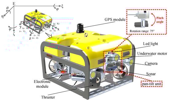
Figure 1.
Graphical representation of ROV coordinate systems and sensor placement.
To accurately describe the motion state of the ROV in space, two right-handed coordinate systems are defined according to the specifications recommended by the International Towing Tank Conference (ITTC) and the Society of Naval Architects and Marine Engineers (SNAME), the fixed coordinate system and the motion coordinate system. These coordinate systems enable a comprehensive description of the ROV’s motion characteristics in space. Specifically, the ROV’s attitude is represented by the Euler angles (i.e., attitude angles) between the fixed and motion coordinate systems, while the velocities, angular velocities, forces, and moments acting on the ROV are expressed in the motion coordinate system. The motion parameters of the ROV are provided in Table 1.

Table 1.
Motion state variables of ROV.
2.2. Software Architecture
The proposed algorithm is developed on the ROS distributed robot operating system, as illustrated in Figure 2. The estimated ROV odometry, pan-tilt angle, sonar images, and global waypoints serve as inputs to the algorithm, which, together with the data preprocessing module, 3D point cloud generation module, and planning and control module, form the underwater three-dimensional spatial perception–planning–control system. Additionally, the focus of this paper does not extend to researching underwater localisation methods. Different underwater localisation methods rely on various sensors and consequently exhibit different localisation errors [8]. Therefore, rather than adopting a specific underwater localisation method, this study investigates the impact of different localisation errors on the proposed perception–planning–control system. This approach enhances the broader applicability of our research.
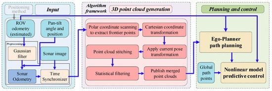
Figure 2.
Framework diagram of the 3D underwater spatial perception–planning–control algorithm.
The estimated ROV odometry data first undergo Gaussian filtering to reduce fluctuations and then are combined with the pan-tilt mechanism’s angle and position relative to the body coordinate system to calculate the sonar’s odometry data. To improve the accuracy of three-dimensional reconstruction, a time synchronisation mechanism filters sonar images and odometry data within a specified time range, which are then input into the 3D point cloud generation module. In the 3D point cloud generation module, sonar image frontiers are first scanned using the polar coordinate system, then the frontier points are converted from polar coordinates to Cartesian coordinates. Next, the sonar odometry data are combined with coordinate transformation to generate a single-frame point cloud in the world coordinate system. Due to the relatively small number of sonar points, the generated single-frame point clouds are continuously integrated to ultimately form the 3D point cloud of the spatial environment. At this stage, the generated point cloud may contain outlier noise, and statistical filtering is applied to remove these outliers. In the planning and control module, the Ego-Planner algorithm integrated in the planning and control module processes spatial 3D point cloud data and generates real-time trajectories by fusing ROV odometry data. This optimisation-based planner computes collision-free path points that constitute the reference trajectory for the ROV’s subsequent motion tracking. Based on the ROV’s current state and position commands, the nonlinear MPC algorithm generates control signals for the six thrusters through rolling optimisation. By continuously executing the above algorithm, the ROV can perceive the surrounding 3D environment, identify obstacle positions and sizes, and navigate around obstacles during global path planning to successfully complete operational tasks.
3. Materials and Methods
3.1. Three-Dimensional Point Cloud Generation
In the ROV structure, the sonar is rigidly mounted to the pan-tilt mechanism, which is in turn fixedly connected to the main body. The pan-tilt mechanism drives the sonar to swing up and down, achieving a wider detection range. For the sonar frontier extraction algorithm, processing is typically performed on the echo intensity of each beam based on the sonar’s raw data [9,10,11]. However, not all sonars provide raw data, while sonar images are a more widely used display method, and image data are easily obtainable. Therefore, targeting the fan-shaped imaging characteristics of sonar, an angle-by-angle scanning frontier extraction algorithm based on the polar coordinate system is proposed, as shown in Figure 3, where the yellow lines represent the contours of the structure, the blue bars illustrate angle-by-angle scanning, and the green lines represent the extracted frontier points.
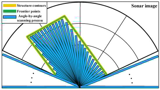
Figure 3.
Polar coordinate sonar processing: angle-wise frontier detection.
The 3D point cloud generation algorithm has two components: the sonar pose estimation algorithm and frontier point extraction algorithm. In the sonar pose estimation algorithm, the position transformation equation is
The attitude transformation equation is
where represents the position of the sonar in world coordinate system, represents the position of the base coordinate system in world coordinate system, is the rotation matrix of the base coordinate system derived from quaternion through the Rodrigues formula, represents the translation from the base coordinate system to sonar coordinate system, and denotes quaternion multiplication. This transformation unifies the coordinate systems by combining the relative pose from the body coordinate system to the sonar coordinate system with the global pose provided by the body odometry, thereby obtaining the position and attitude of the sonar point cloud in the world coordinate system. In the position transformation equation, the rotation matrix calculation employs
In the angle-by-angle scanning frontier extraction algorithm based on the polar coordinate system, further point cloud generation processing is performed based on the images returned by sonar. The relationship for the frontier points between the polar coordinate system and Cartesian coordinate system can be expressed as
where represents the scanning origin in the sonar image coordinate system, defined as , where and are the width and height of image, respectively.
The frontier points are filtered according to the following conditions:
where represents the set of valid scanning angles, and represents the threshold value. It should be noted that the CFAR method is not employed in this study. Since the CFAR approach involves multiple computational steps, the direct thresholding method is more suitable for meeting the real-time requirements essential for obstacle avoidance manoeuvres.
The specific scanning process for frontier points is shown in Algorithm 1.
| Algorithm 1 Polar Frontier Detection |
|
After completing the extraction of frontier points, further calculations are performed to obtain the point cloud. The coordinates of frontier points in local coordinate system of the underwater robot are calculated as follows:
where is the initial depth value of the sonar. The radial resolution is defined as , where represents the maximum range of sonar.
Then, rigid body transformation applied to map the point cloud in the local coordinate system to the point cloud in the world coordinate system can be expressed as
where is the translation vector, representing the sonar’s position in the global frame. The rotation matrix can be constructed in Z-Y-X order as
The rotation matrices of each axis can be expressed as
Due to noise in the sonar image, several outlier points may appear in the generated point cloud within the world coordinate system. A denoising algorithm based on local density analysis (i.e., statistical filtering algorithm) is used to filter the generated point cloud. Firstly, the algorithm constructs a fixed-radius neighbourhood for each point and counts the number of other points in that neighbourhood as a local density value. Subsequently, by setting a density threshold, points with density lower than normal data are filtered out as outliers, thereby removing noise data while preserving the overall structure and key features of the data. The formula related to statistical filtering algorithm is as follows:
where represents the Euclidean distance (L2 norm) between points and , represents the k-nearest neighbour set of point , i.e., the k points closest to , represents the average neighbourhood distance of point , used to measure the distribution of that point with its neighbouring points. If is large, it indicates that the distance between point and its neighbourhood points is far, leading to its classification as an outlier. Additionally, is the mean of the average neighbourhood distances of all points, is the standard deviation of the average neighbourhood distances of all points, and is an adjustable parameter used to control the strictness of outlier determination. The larger is, the more lenient the determination condition should be; the smaller is, the stricter the determination condition should be. Therefore, serves as the determination threshold for outliers. If is less than this threshold, is considered a normal point; otherwise, it is considered an outlier. Further filtering is applied to points greater than a certain depth value to filter out points that do not conform to environmental structural features, as described by the following formula:
where is the final processed point cloud, is the point cloud after statistical filtering, is the z-axis coordinate of the point cloud in the world coordinate system, and is the depth value threshold.
3.2. Motion Control Strategy
In this study, the Ego-Planner path planning algorithm [12] is employed to plan local paths among global waypoints, while a nonlinear MPC algorithm is utilised to track the planned paths.
Ego-Planner is a 3D spatial trajectory planning framework designed to generate safe, smooth, and dynamically feasible trajectories in complex environments. In contrast to conventional planning methods, Ego-Planner eliminates the need for Environmental Signed Distance Field (ESDF) maps. Instead, it directly performs collision detection and obstacle avoidance using point cloud data, significantly reducing computational complexity and improving system real-time performance and robustness. The core philosophy of this framework lies in its phased optimisation strategy, which progressively generates trajectories that satisfy smoothness, static obstacle avoidance, and dynamic feasibility requirements.
The Ego-Planner planning workflow comprises the following steps:
- Initial Trajectory Generation: A minimum-jerk or minimum-snap trajectory connecting the start and goal points is initially generated without considering obstacles, satisfying only boundary state constraints.
- Collision Detection and Penalty: Using point cloud data, the A* algorithm identifies collisions between the initial trajectory and obstacles. A refined collision penalty cost function is formulated to ensure effective obstacle avoidance during subsequent optimisation.
- Trajectory Optimisation Model: The trajectory is parameterised using B-spline curves, and an optimisation model incorporating smoothness, static obstacle avoidance, and dynamic feasibility is established. Iterative optimisation produces collision-free, smooth trajectories.
- Temporal Reallocation and Trajectory Refinement: When dynamic feasibility constraints are violated in specific trajectory segments, Ego-Planner reallocates temporal parameters and reconstructs the optimisation model to incorporate smoothness, dynamic constraints, and curve fitting, thereby generating executable trajectories.
In nonlinear MPC algorithms [13,14,15], future state predictions are based on the established kinematics and dynamics models of the ROV along with system inputs. The core principle of this approach involves integrating three fundamental components—predictive modelling, receding horizon optimisation, and feedback correction—to achieve effective control of complex systems.
The Model Predictive Control framework primarily consists of the following key components:
- Predictive Model: As the foundation of MPC, the predictive model characterises the system’s dynamic behaviour. It utilises the current state and future control inputs to forecast output states over a defined prediction horizon.
- Receding Horizon Optimisation: Unlike conventional global optimal control strategies, MPC employs a receding horizon approach. At each sampling instant, it computes the optimal control sequence over a finite prediction window by minimising a predefined cost function, subject to the current system state and imposed constraints.
- Feedback Correction: Discrepancies between predicted and actual system outputs may result from model inaccuracies, external disturbances, or system nonlinearities. To mitigate these effects, MPC integrates real-time feedback by measuring output errors and adjusting subsequent predictions accordingly. This mechanism improves robustness to uncertainties and ensures reliable performance across varying operational conditions.
The kinematic and dynamic models of the ROV are established as follows. The transformation relationships between linear and angular velocities and the spatial orientation are given as follows:
where matrices and represent the transformation of ROV from the vehicle-fixed coordinate system to the inertial reference frame, which can be formulated using Euler angles as
Since the pitch and roll angles remain unregulated during motion and are assumed to be stabilised through initial trim adjustments, the aforementioned model can be simplified to derive the ROV kinematic model:
where , , and represents the transformation matrix.
Following the dynamic model established by Fosson et al. [16] for underwater vehicles, the ROV dynamics can be expressed as
where denotes the inertia matrix (including added mass), represents the Coriolis and centripetal matrix, is the hydrodynamic damping matrix, contains restoring forces from buoyancy and gravity, and defines the generalised force vector generated by thrusters. The added mass matrix is related to the acceleration of the ROV during motion and can be determined using empirical formulas established in submarine design methodology. The Coriolis and centripetal matrix is dependent on both the physical parameters of the ROV and the added mass matrix . The hydrodynamic damping matrix , which characterises the fluid resistance forces and moments acting on the ROV, is determined through computational fluid dynamics (CFD) simulation software. Due to the relatively small volume and mass of the pan-tilt mechanism compared to the overall ROV system, its rotational effects are reasonably neglected in the modelling process, thereby simplifying the dynamic model while maintaining sufficient accuracy for control purposes.
In this study, serves as the control input, with its components defined as , where , , and indicate control forces along the body-fixed axes, and represents control moments about the corresponding axes. Let denote the input force signals of eight thrusters, and the thruster allocation can be formulated as
The relationship between and the individual thrusts from the six thrusters can be derived using positional vector analysis relative to the ROV’s body-fixed origin, as follows:
where denotes the thrust allocation matrix for the ROV.
Next, the objective function for the MPC algorithm is constructed. During receding horizon optimisation, the future motion states of the ROV are predicted using the formulated objective function in conjunction with the established ROV dynamics model. The objective function balances position error (i.e., the deviation between the current and target states) and control effort, with their relative contributions regulated by predefined weighting coefficients. The objective function is mathematically represented as
where represents the real-time position and yaw angle of the ROV, denotes the reference waypoints generated by the Ego-Planner local path planner for tracking, and and are the weighting coefficients for positional error term and control input term, respectively. The dynamic performance and steady-state stability of the ROV motion can be adjusted by tuning the weight ratio.
4. Experimental Validation
4.1. Three-Dimensional Reconstruction Experiment in Stationary Mode
To evaluate the effectiveness of the three-dimensional reconstruction method based on the oscillatory forward-looking sonar, experiments were conducted in a river beneath a bridge, as shown in Figure 4.
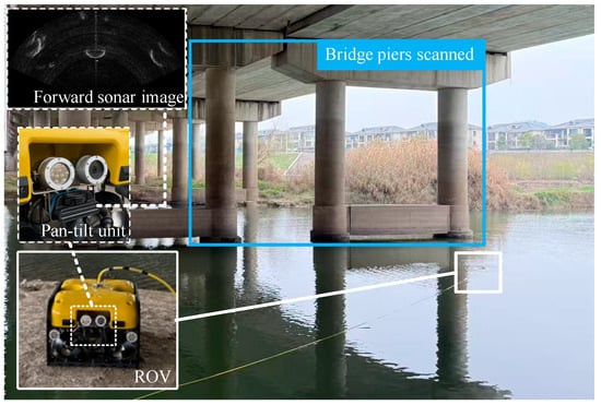
Figure 4.
Experimental scene and sonar image for 3D reconstruction.
The sonar system employed in the experiment features a 10 m range, with a 70-degree horizontal field of view and a 12-degree vertical field of view. The system comprises 512 beams, achieving an angular resolution of 0.6 degrees. During the experiment, the ROV scanned the bridge piers with position and attitude control enabled to ensure that its position remained fixed and its attitude unchanged. The pan-tilt angle was varied within a range of −30 degrees to 5 degrees, while the forward-looking sonar continuously produced sonar images. A laser rangefinder was used from the shore to measure the diameter of the bridge piers and the distance between them, serving as a reference for comparison with the three-dimensional reconstruction results.
Figure 5 presents the three-dimensional reconstruction results of the bridge piers. The gridded surface denotes the water level, with each cell corresponding to a defined spatial resolution. The point cloud is colour-coded to represent variations in depth. The reconstruction successfully captures all three bridge piers included in the scan. By fitting the point cloud data, the diameter of each pier and the inter-pier distances can be estimated, as shown in Table 2.
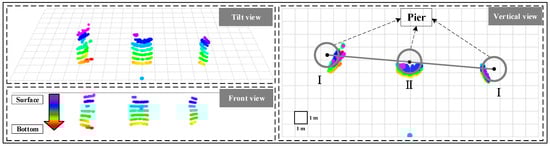
Figure 5.
Three-dimensional graphical representation of bridge pier 3D reconstruction.
Table 2.
Comparison between measured and estimated values for pier diameters and inter-pier distances.
The diameters of the bridge piers were measured three times using a laser rangefinder. The average pier diameter was 1.973 m, with the average distances between Pier I and Pier II and between Pier II and Pier III measuring 6.178 m and 6.702 m, respectively. The pier diameter estimated from the point cloud data was 2.112 m, with distances between Pier I and Pier II and between Pier II and Pier III measured as 6.300 m and 6.499 m, respectively. The corresponding errors were 0.139 m, 0.122 m, and 0.203 m. These results indicate that the maximum experimental error was 0.203 m. In the Ego-Planner path planning algorithm, incorporating an obstacle expansion margin can mitigate the impact of three-dimensional reconstruction errors. Consequently, the oscillatory forward-looking sonar demonstrates effectiveness in three-dimensional structural reconstruction and mapping, with the generated point cloud data suitable for obstacle avoidance and motion control.
4.2. Three-Dimensional Reconstruction of Water Tank Environment and Autonomous Obstacle Avoidance Experiments
To assess the autonomous obstacle avoidance and motion control capabilities of the ROV based on 3D reconstruction point cloud, simulation experiments were conducted in the ROS Gazebo environment. The simulation experiments were conducted on a system running Ubuntu 20.04, equipped with an AMD Ryzen 9 5900HX CPU, 32 GB of RAM, and an NVIDIA GeForce RTX 3080 GPU. The sonar plugin was developed based on the work of Choi et al. [17,18]. During runtime, the proposed algorithm exhibited CPU load fluctuations around 70%. The fundamental parameters of the ROV used in the ROS Gazebo environment are listed in Table 3.
Table 3.
ROV rigid-body parameters.
The parameter settings of the Ego-Planner local path planner are summarised in Table 4.
Table 4.
Ego-Planner algorithm parameters.
The parameter settings of the MPC algorithm are summarised in Table 5.
Table 5.
MPC algorithm parameters.
In the simulation environment, a pool was constructed with dimensions of 20 m (length), 10 m (width), and 10 m (depth). Two square-section pillars, each with a side length of 1 m, were placed in the pool as obstacles, as illustrated in Figure 6. The underwater robot started from the initial point and completed its cruise by sequentially following predefined global waypoints. A rectangular trajectory with three distinct depth variations was designed for the simulation experiment. Odometry data with standard deviations of 0 m, 0.25 m, and 0.5 m were used for three-dimensional reconstruction to validate the robustness of the proposed 3D spatial perception, planning, and control system. It is important to note that since the depth sensor and electronic compass provide high-precision depth and yaw measurements, no noise was added to these values. Instead, noise was introduced only to the x and y position coordinates. Additionally, an acoustic model, such as multi-path reflection, was not incorporated during simulation experiments. This decision was based on empirical observations from physical experiments, where shadow artefacts caused by multi-path reflection appeared behind obstacles when the pan-tilt mechanism was in a horizontal position. These reflection-induced shadows exhibited lower intensities compared to actual shadows. Since the proposed method only processes the frontier points, multi-path reflection did not affect the three-dimensional reconstruction results. Furthermore, when the pan-tilt mechanism was tilted downward, the influence of multi-path reflections was further diminished. Based on these considerations, acoustic modelling (mainly multi-path reflection) was not incorporated for the sonar simulation.

Figure 6.
Schematic diagram of the simulation test environment.
Figure 7 panels (a), (d), and (g) illustrate the ROV motion trajectories under varying levels of standard deviation noise. Green spheres represent the ROV’s starting position, red spheres denote predefined global waypoints, and red dashed lines connect the command positions generated by the Ego-Planner path planning algorithm. Blue lines trace the ROV’s actual trajectory.
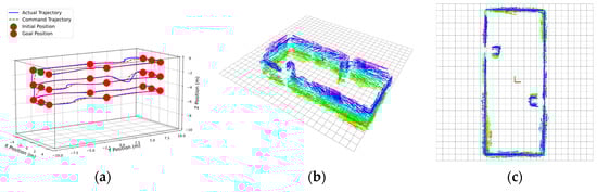
Figure 7.
Results with odometry σ = 0/0.25/0.5 m: (a,d,g) trajectories; (b,c,e,f,h,i) 3D point clouds.
The results demonstrate that the ROV successfully followed the rectangular trajectory at three different depths. When the oscillatory forward-looking sonar detected obstacles ahead, it promptly planned alternative paths to avoid them. The nonlinear MPC effectively tracked the command positions, enabling successful task completion.
An examination of the three-dimensional reconstruction point cloud reveals that as odometry noise increases, the point cloud becomes increasingly disordered. This indicates a gradual decline in the accuracy of estimated obstacle positions and dimensions, necessitating larger obstacle expansion margins in the Ego-Planner algorithm to prevent potential collisions.
Figure 8, Figure 9 and Figure 10 illustrate the ROV state information under different odometry standard deviations. The odometry curves demonstrate the ROV’s effective tracking of command positions. During trajectory turns, minor overshoots occur; however, the system stabilises quickly. The velocity curves indicate that the ROV’s maximum velocity is approximately 0.45 m/s. Notably, as the odometry standard deviation increases, neither the maximum nor the average velocity exhibit significant variation. This stability is attributed to the robust state estimation and control capabilities of the Ego-Planner path planning algorithm and the MPC algorithm.
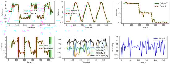

Figure 8.
Time-series plots of ROV state variables under perfect odometry assumption (σ = 0 m).

Figure 9.
Time-series plots of ROV state variables under moderate odometry noise (σ = 0.25 m).
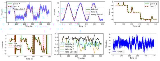
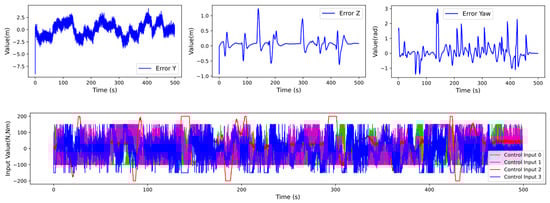
Figure 10.
Time-series plots of ROV state variables with severe odometry uncertainty (σ = 0.5 m).
The error curves were obtained by subtracting noisy odometry values from the command positions, and these differences were incorporated into the objective function of the nonlinear MPC controller. The error curves show that x, y, and z position errors and yaw angle errors fluctuate around zero, indicating the controller’s ability to promptly correct position deviations. It is worth noting that at the initial time, y, z, and yaw errors appear larger, as the task has not yet started, and the differences are computed between odometry and the origin coordinates. This approach simplifies program implementation and does not affect algorithm performance.
The control input curves demonstrate that as odometry noise increases, control inputs exhibit greater oscillations, which may lead to increased energy consumption. However, no filtering algorithm was applied in order to preserve critical state information and maintain the effectiveness of obstacle avoidance and motion control.
In the simulation experiments, ten trials were conducted for each level of odometry standard deviation to evaluate the impact of localisation errors on obstacle avoidance success rates. The results are summarised in Table 6. When the standard deviation was 0 m, the obstacle avoidance success rate was 100%; in contrast, it dropped to 30% at a standard deviation of 0.5 m.
Table 6.
Statistical analysis of avoidance success rates vs. odometry uncertainty (σ = 0–0.5 m).
The data demonstrate that obstacle avoidance success rates progressively decline as the standard deviation increases. This degradation is primarily attributed to the adverse influence of highly inaccurate localisation information on the nonlinear MPC algorithm. Excessive positioning errors may cause the ROV to deviate from its intended trajectory, ultimately resulting in potential collisions with obstacles. It is also worth noting that although the positioning error has an impact on the results of 3D reconstruction, the path can be generated by setting a suitable obstacle expansion distance, which also shows the robustness of the proposed system to positioning errors.
5. Conclusions and Future Perspectives
This paper presents a three-dimensional reconstruction method for underwater environments based on an oscillatory forward-looking sonar, which is integrated with the Ego-Planner path planning algorithm and nonlinear MPC algorithm to form a comprehensive underwater 3D spatial perception–planning–control system. The primary conclusions are as follows:
- (1)
- The oscillatory forward-looking sonar extends the perception range of traditional two-dimensional sonar to a 75-degree pitch angle through a pan-tilt mechanism, enabling effective 3D underwater environment perception at a significantly lower cost than professional 3D sonar systems.
- (2)
- The polar coordinate-based sonar image feature extraction method captures complete contour frontier information, thereby enhancing the accuracy and reliability of 3D reconstruction.
- (3)
- Validated through outdoor bridge pier scanning experiments, the proposed method achieves a maximum measurement error of 0.203 m, enabling effective 3D reconstruction and mapping of underwater structures such as bridge piers.
- (4)
- Obstacle avoidance experiments conducted in the Gazebo simulation environment show that the 3D point cloud generated by the oscillatory forward-looking sonar provides effective environmental input for the Ego-Planner path planning algorithm, enabling autonomous obstacle avoidance and motion control for underwater vehicles.
- (5)
- The system demonstrates robustness to localisation errors, achieving obstacle avoidance success rates of 100%, 60%, and 30% under localisation errors of 0 m, 0.25 m, and 0.5 m, respectively.
- (6)
- As localisation errors increase, control inputs exhibit significant oscillations, energy consumption rises, and obstacle avoidance success rates decline significantly, highlighting the strong dependence of system performance on localisation precision.
In summary, the proposed three-dimensional reconstruction method and underwater 3D spatial perception–planning–control system provide a novel technological solution for autonomous operations in complex underwater environments. This approach offers advantages such as a simple structure, low cost, and high reliability and presents broad application prospects in underwater infrastructure inspection and marine environmental monitoring.
Despite the promising experimental results, several challenges and opportunities for improvement remain in practical applications. Future research directions include the following:
- (1)
- Point Cloud Registration: The current system relies on accurate pose information for point cloud integration. Future work will focus on advanced point cloud registration algorithms, such as Iterative Closest Point (ICP) and Normal Distributions Transform (NDT), to reduce dependence on external localisation systems. Considering the sparse and noisy characteristics of underwater sonar point cloud, the study will explore feature extraction and matching techniques tailored to underwater environments, with the goal of developing robust registration algorithms to enhance 3D reconstruction accuracy and reliability, particularly under low-precision localisation conditions.
- (2)
- Point Cloud Storage and Management: Efficient point cloud storage and management are critical for maintaining system performance. Future work will explore large-scale 3D environmental mapping, employing data structures such as KD trees, octrees, and voxel grids in underwater settings. It will also develop compression algorithms for sparse point clouds to reduce memory usage and computational overhead. Additionally, incremental environmental modelling methods will be investigated to enable real-time map updates and optimisation, supporting long-term, large-scale underwater autonomous operations while addressing the computational efficiency limitations of current systems.
- (3)
- Optimisation of the Model Predictive Control Algorithm: Continued tuning of MPC parameters aims to reduce motion oscillations and improve 3D reconstruction performance. In response to underwater disturbances such as currents and waves, the study will incorporate disturbance observers and compensation mechanisms into the MPC framework to enhance its robustness against environmental disturbances. In addition, learning-based MPC methods will be explored, leveraging historical control data to optimise prediction models and control parameters, thus laying the foundation for high-quality 3D environmental reconstruction.
- (4)
- Acoustic Modelling: Virtual simulation experiments are efficient for rapidly validating proposed methods. However, current simulation approaches do not fully capture acoustic characteristics. This represents a significant challenge in terms of both hardware performance and algorithmic complexity. Future work will explore efficient acoustic modelling methods to further enhance the fidelity of simulation experiments and improve the efficiency of algorithm development.
Through continued research in these directions, significant improvements in performance and broader applicability of the underwater 3D spatial perception–planning–control system based on oscillatory forward-looking sonar are expected. This advancement will facilitate the practical deployment of the technology in complex underwater environments, offering more reliable and efficient technical support for underwater infrastructure inspection, marine environmental monitoring, and related operations.
Author Contributions
Conceptualisation, H.Z., Z.Z., H.W. and Z.C.; data curation, H.Z. and Y.R.; formal analysis, S.T. and Z.Z.; methodology, H.Z., H.W. and Z.C.; software, H.Z. and Y.Z.; resources, H.W. and Z.C.; writing—original draft, H.Z.; writing—review and editing, H.Z., Y.R., S.T. and Y.Z.; supervision, Z.Z., H.W. and Z.C. All authors have read and agreed to the published version of the manuscript.
Funding
This work was funded by the Zhejiang Provincial Science and Technology Program, China, grant number 2024C03036.
Data Availability Statement
The original contributions presented in this study are included in the article. Further inquiries can be directed to the corresponding author(s).
Conflicts of Interest
Authors Zhixin Zhou, Haiteng Wu and Shaohua Tian were employed by the company Hangzhou Shenhao Technology Co., Ltd. The remaining authors declare that the research was conducted in the absence of any commercial or financial relationships that could be construed as a potential conflict of interest.
References
- Lin, M.; Yang, C. Ocean Observation Technologies: A Review. Chin. J. Mech. Eng. 2020, 33, 32. [Google Scholar] [CrossRef]
- Teng, S.; Liu, A.; Ye, X.; Wang, J.; Fu, J.; Wu, Z.; Chen, B.; Liu, C.; Zhou, H.; Zeng, Y.; et al. Review of Intelligent Detection and Health Assessment of Underwater Structures. Eng. Struct. 2024, 308, 117958. [Google Scholar] [CrossRef]
- Elmezain, M.; Saad Saoud, L.; Sultan, A.; Heshmat, M.; Seneviratne, L.; Hussain, I. Advancing Underwater Vision: A Survey of Deep Learning Models for Underwater Object Recognition and Tracking. IEEE Access 2025, 13, 17830–17867. [Google Scholar] [CrossRef]
- Rout, D.K.; Kapoor, M.; Subudhi, B.N.; Thangaraj, V.; Jakhetiya, V.; Bansal, A. Underwater Visual Surveillance: A Comprehensive Survey. Ocean. Eng. 2024, 309, 118367. [Google Scholar] [CrossRef]
- Tang, Z.; Lu, J.; Wang, Z.; Ma, G. Three Dimensional Height Information Reconstruction Based on Mobile Active Sonar Detection. Appl. Acoust. 2020, 169, 107459. [Google Scholar] [CrossRef]
- Sadjoli, N.; Yiyu, C.; Lee, G.S.G.; Elhadidi, B. Effectiveness of 3D PCD Reconstruction Using Orthogonal Multiple Sonar Fusion on Frame and Surface Type Objects. In Proceedings of the OCEANS 2022, Hampton Roads, VA, USA, 17–20 October 2022; pp. 1–6. [Google Scholar]
- Kim, B.; Kim, J.; Cho, H.; Kim, J.; Yu, S.-C. AUV-Based Multi-View Scanning Method for 3-D Reconstruction of Underwater Object Using Forward Scan Sonar. IEEE Sens. J. 2020, 20, 1592–1606. [Google Scholar] [CrossRef]
- Wu, H.; Chen, Y.; Yang, Q.; Yan, B.; Yang, X. A Review of Underwater Robot Localization in Confined Spaces. J. Mar. Sci. Eng. 2024, 12, 428. [Google Scholar] [CrossRef]
- Mu, X.; Yue, G.; Zhou, N.; Chen, C. Occupancy Grid-Based AUV SLAM Method with Forward-Looking Sonar. J. Mar. Sci. Eng. 2022, 10, 1056. [Google Scholar] [CrossRef]
- Wang, J.; Chen, F.; Huang, Y.; McConnell, J.; Shan, T.; Englot, B. Virtual Maps for Autonomous Exploration of Cluttered Underwater Environments. IEEE J. Ocean. Eng. 2022, 47, 916–935. [Google Scholar] [CrossRef]
- Cheng, C.; Wang, C.; Yang, D.; Liu, W.; Zhang, F. Underwater Localization and Mapping Based on Multi-Beam Forward Looking Sonar. Front. Neurorobot. 2022, 15, 801956. [Google Scholar] [CrossRef] [PubMed]
- Zhou, X.; Wang, Z.; Ye, H.; Xu, C.; Gao, F. EGO-Planner: An ESDF-Free Gradient-Based Local Planner for Quadrotors. IEEE Robot. Autom. Lett. 2021, 6, 478–485. [Google Scholar] [CrossRef]
- Li, W.; Zhang, X.; Wang, Y.; Xie, S. Comparison of Linear and Nonlinear Model Predictive Control in Path Following of Underactuated Unmanned Surface Vehicles. J. Mar. Sci. Eng. 2024, 12, 575. [Google Scholar] [CrossRef]
- Bashi, O.I.D.; Jameel, S.M.; Sabry, A.H. Trajectory Optimization to Minimize Fuel Usage for Positioning Guide by a Nonlinear Model Predictive Control for Underwater Robots. Ocean. Eng. 2024, 300, 117271. [Google Scholar] [CrossRef]
- Hu, Y.; Li, B.; Jiang, B.; Han, J.; Wen, C.-Y. Disturbance Observer-Based Model Predictive Control for an Unmanned Underwater Vehicle. J. Mar. Sci. Eng. 2024, 12, 94. [Google Scholar] [CrossRef]
- Fossen, T.I. Handbook of Marine Craft Hydrodynamics and Motion Control; John Wiley & Sons: Hoboken, NJ, USA, 2011; ISBN 978-1-119-99149-6. [Google Scholar]
- Choi, W.-S. Ray-Based Physical Modeling and Simulation of Multibeam Sonar for Underwater Robotics in ROS-Gazebo Framework. Sensors 2025, 25, 1516. [Google Scholar] [CrossRef] [PubMed]
- Choi, W.-S.; Olson, D.R.; Davis, D.; Zhang, M.; Racson, A.; Bingham, B.; McCarrin, M.; Vogt, C.; Herman, J. Physics-Based Modelling and Simulation of Multibeam Echosounder Perception for Autonomous Underwater Manipulation. Front. Robot. AI 2021, 8, 706646. [Google Scholar] [CrossRef] [PubMed]
Disclaimer/Publisher’s Note: The statements, opinions and data contained in all publications are solely those of the individual author(s) and contributor(s) and not of MDPI and/or the editor(s). MDPI and/or the editor(s) disclaim responsibility for any injury to people or property resulting from any ideas, methods, instructions or products referred to in the content. |
© 2025 by the authors. Licensee MDPI, Basel, Switzerland. This article is an open access article distributed under the terms and conditions of the Creative Commons Attribution (CC BY) license (https://creativecommons.org/licenses/by/4.0/).