1. Introduction
Cavitation is a complex multiphase phenomenon that occurs when local fluid pressure drops below the vapor pressure, leading to the formation of vapor cavities. These cavities grow in low-pressure regions and collapse when they encounter higher-pressure zones, resulting in significant pressure fluctuations, turbulence, and potentially destructive effects such as erosion, noise, and vibration. Cavitation plays a crucial role in various engineering applications, including ship propellers, hydrofoils, and turbomachinery, where accurate prediction is essential for improving performance and structural reliability. Computational fluid dynamics (CFD) has been widely employed to simulate cavitating flows, yet the strong coupling between turbulence and phase change remains a major challenge in numerical modeling.
De la Cruz-Avila et al. [
1] investigated cavitation within a rectangular-profile Venturi tube using numerical simulations and evaluates four turbulence models:
realizable,
RNG, and
SST. The research highlighted the challenges in accurately predicting vapor cloud formation due to the intricate interactions between turbulence and phase change phenomena, underscoring the need for precise turbulence modeling in cavitating flows. Salvatore et al. [
2] presented a benchmark study comparing seven computational models, including Reynolds-averaged Navier–Stokes (RANS), large eddy simulation (LES), and boundary element method (BEM), applied to the INSEAN E779A propeller. The findings reveal significant variations in predicting cavitation phenomena, emphasizing the challenges in modeling the strong coupling between turbulence and phase change in propeller applications. Similarly, Zhu et al. [
3] evaluated the performance of various cavitation models in simulating water flow, focusing on their ability to incorporate vapor-phase transport. The study identified limitations in existing models, particularly in capturing the phase change processes accurately, highlighting the ongoing challenges in CFD simulations of cavitating flows. Pipp et al. [
4] discussed the complexities involved in simulating cavitation reactors, noting that cavitation exhibits intricate flow features even in simple geometries. The authors emphasized that poor CFD approaches can lead to misinterpretations and suboptimal engineering solutions, stressing the importance of accurately modeling the interplay between turbulence and phase change.
To enhance the accuracy of cavitation simulations, various mass transfer models have been developed to describe the phase transition between liquid and vapor phases. The Kunz model is a widely used approach that introduces empirical source terms to control the vaporization and condensation processes based on local pressure conditions. This model is computationally efficient and provides stable solutions for engineering applications. Cao et al. [
5] employed the Kunz cavitation model, among others, to simulate cavitating flow in a centrifugal pump. The research demonstrated that the Kunz model effectively captures cavitation characteristics while maintaining computational efficiency, making it suitable for engineering applications where stable and efficient simulations are required. Additionally, Hanimann et al. [
6] investigated various cavitation models, including the Kunz model, for steady-state CFD simulations. The study found that the Kunz model exhibited favorable behavior concerning numerical stability and computational efficiency, highlighting its suitability for engineering applications requiring reliable and efficient simulations.
However, the Kunz model’s ability to resolve transient cavitation dynamics is limited, as it often predicts a more diffused cavity structure and struggles to capture small-scale turbulent features such as re-entrant jets and vortex shedding. The Merkle model adopts a similar pressure-based framework but incorporates a more refined formulation for phase change dynamics, allowing for improved predictions of steady cavitation behavior. While the Merkle model provides a balance between computational cost and accuracy, it still faces difficulties in resolving unsteady shedding behavior and turbulence–cavitation interactions in highly dynamic flow environments. Liu [
7] compared the performance of the Kunz, Merkle, and Schnerr–Sauer cavitation models in simulating unsteady cavitation around a Clark-Y hydrofoil. The findings indicated that both the Merkle and Schnerr–Sauer models outperform the Kunz model in capturing unsteady cavitation phenomena, closely aligning with experimental observations. The Kunz model demonstrated limitations in resolving transient cavitation dynamics, often predicting more diffused cavity structures and inadequately capturing small-scale vortices, including re-entrant jets and vortex shedding. In contrast, the Merkle model provided more accurate simulations of unsteady cavitation flows, although it still faced challenges in fully resolving complex turbulence-cavitation interactions. Tran et al. [
8] evaluated the applicability of mass transfer cavitation models, specifically the Kubota and Merkle models, for simulating cavitating flows around a NACA66 hydrofoil under both steady and unsteady conditions. The study found that the Merkle model offered improvements in simulating cavitating flows, particularly in steady-state scenarios. However, challenges persisted in accurately predicting unsteady cavitation behaviors, such as cavity shedding and turbulence–cavitation interactions, highlighting the need for further refinement in modeling approaches to capture these complex dynamics effectively.
The Schnerr–Sauer model, derived from the Rayleigh–Plesset equation, explicitly accounts for bubble dynamics in the cavitation process. This model offers a more accurate representation of cavitation growth and collapse by considering individual vapor bubbles’ expansion and contraction. Sauer and Schnerr [
9] discussed the development of a cavitation model grounded in bubble dynamics, emphasizing the Schnerr–Sauer model’s foundation on the Rayleigh–Plesset equation. The research highlighted that the Schnerr–Sauer model effectively captures the growth and collapse of vapor bubbles by considering their expansion and contraction, leading to more accurate predictions of cavitation phenomena. The study also noted that the model’s ability to scale bubble growth rates allows for controlled simulation of vapor distribution within the flow. Hong et al. [
10] proposed enhancements to the Schnerr–Sauer model to improve its predictive capabilities for cavitating flows. By refining the original model’s parameters, the study demonstrated improved accuracy in simulating cavitation growth and collapse dynamics. The modified model continues to rely on the Rayleigh–Plesset equation to account for individual bubble behavior, thereby offering a detailed representation of bubble dynamics within cavitating flows. Consequently, the Schnerr–Sauer model is particularly effective in capturing rapid phase transition effects and unsteady cavitation structures. However, its computational expense is significantly higher due to the increased complexity of its formulation.
Cavitating flows exhibit inherently turbulent characteristics, making turbulence modeling a critical aspect of CFD simulations. The RANS model is one of the most commonly employed turbulence modeling approaches due to its relatively low computational cost. By averaging the effects of turbulence over time, RANS reduces the complexity of solving the full Navier–Stokes equations. However, this time-averaging process leads to the suppression of transient flow structures, making it less suitable for accurately predicting cavitation-induced turbulence, vortex interactions, and unsteady shedding behavior. To overcome these limitations, the partially averaged Navier–Stokes (PANS) model has been introduced as a hybrid approach between RANS and LES. Geng and Escaler [
11] evaluated the effectiveness of various RANS turbulence models in predicting unsteady cavitation phenomena. The findings indicated that while RANS models are computationally efficient, they often struggle to capture transient flow structures such as vortex shedding and cavitation-induced turbulence. This limitation arises from the inherent time-averaging approach of RANS, which suppresses the unsteady characteristics essential for accurate cavitation prediction. Similarly, Naseri et al. [
12] assessed the predictive capabilities of different turbulence models, including RANS and LES, in simulating incipient cavitation within a step nozzle. The study revealed that RANS models, such as the realizable
SST, and Reynolds Stress model, failed to predict cavitation due to their limitations in capturing low-pressure vortex cores. In contrast, the LES WALE model successfully predicted cavitation by capturing shear layer instability and vortex shedding, highlighting the necessity for models that can resolve transient flow features. Hu et al. [
13] introduced a modification to the PANS model aimed at improving simulations of unsteady cavitating flows. The modified PANS model demonstrates enhanced capability in capturing transient cavitation dynamics, including vortex interactions and unsteady shedding behavior, offering a balance between computational cost and accuracy. Additionally, Huang et al. [
14] applied a modified PANS model to simulate transient cavitating turbulent flows. The results showed that the modified PANS model effectively captures unsteady cavitation phenomena, such as cavity shedding and turbulence-cavitation interactions, addressing the limitations observed in traditional RANS models.
Unlike RANS, which models all turbulence scales, or LES, which resolves large-scale turbulence while modeling only small-scale effects, PANS dynamically adjusts the turbulence resolution based on local flow conditions. By selectively resolving a portion of the turbulence spectrum, PANS provides an improved representation of unsteady flow structures while maintaining a manageable computational cost. This makes it particularly useful for cavitating flow simulations, where capturing transient phenomena such as cavity shedding and re-entrant jet formation is crucial. This study aimed to investigate the influence of different cavitation models, specifically the Kunz, Merkle, and Schnerr–Sauer models, on the numerical prediction of cavitating flows around a hemispherical head-form body. Additionally, the impact of turbulence modeling approaches, including RANS and PANS, on cavitation dynamics would be examined.
The hemispherical head-form body has been widely used as a benchmark geometry for cavitation studies due to its well-documented experimental data and its ability to produce strong cavitation effects. By systematically analyzing the cavity formation process, shedding behavior, and turbulence interactions, this study sought to evaluate the predictive capabilities of different modeling approaches. The findings of this research will provide valuable insights into the selection of appropriate cavitation and turbulence models for engineering applications, thereby contributing to the advancement of high-fidelity CFD simulations of cavitating flows. Recent studies, such as Ge et al. [
15], have begun to address the coupling between thermal and hydrodynamic effects in cavitating flows, proposing new modeling strategies to capture this interaction. Although the present study focused on isothermal conditions, these developments offer valuable directions for future research.
This paper is organized as follows:
Section 2 outlines the numerical methods and computational setup, detailing the governing equations, cavitation models, turbulence modeling approaches, and computational framework.
Section 3 presents the results and discussion, highlighting the comparative analysis of pressure distribution, cavitation structures, turbulence characteristics, and unsteady shedding behavior across different models. Finally,
Section 4 provides a summary of the key findings and discusses potential directions for future research.
2. Numerical Methods and Computational Setup
2.1. Governing Equations
In this study, numerical simulations were performed using the Reynolds-averaged Navier–Stokes (RANS) and partially averaged Navier–Stokes (PANS) models to analyze turbulent flow characteristics. The governing equations for each approach are presented below.
2.1.1. Reynolds-Averaged Navier–Stokes (RANS)
The RANS formulation approximates turbulence by decomposing the flow variables into mean and fluctuating components, applying time-averaging to remove small-scale turbulent fluctuations. This approach is computationally efficient and widely used in engineering applications due to its ability to capture dominant flow structures. The governing equations for mass and momentum conservation in the RANS framework are expressed as follows:
where
and
represent the time-averaged velocity and pressure, respectively. The subscript
indicates the mixture phase, for which the density and viscosity are calculated using volume–fraction-weighted averages based on the Volume of Fluid (VOF) method [
16].
The Reynolds stress tensor
accounts for the effect of turbulent fluctuations on the mean flow and is modeled using the Boussinesq approximation:
where
denotes the strain rate tensor derived from the time-averaged velocity field, and
represents the turbulent kinetic energy. The eddy viscosity
is defined as:
where
is the specific dissipation rate.
The turbulence closure in this study is achieved using the
shear stress transport (SST) model, which effectively combines the near-wall accuracy of the
model with the free-stream robustness of the
model. This hybrid approach improves prediction accuracy in complex flow scenarios, including flow separation and adverse pressure gradients. Further details on the derivation of these equations can be found in the literature [
16,
17,
18].
2.1.2. Partially Averaged Navier–Stokes (PANS)
The PANS model bridges the gap between RANS and DNS by resolving a portion of the turbulence spectrum while modeling the unresolved scales. This approach enhances the representation of turbulent structures without the computational cost of fully resolving all scales. The governing equations for the PANS method consist of the filtered continuity and momentum equations:
where
and
denote the partially averaged velocity and pressure, respectively. The sub-filter scale (SFS) stress tensor
accounts for the influence of unresolved turbulence on the resolved field and is modeled using the Boussinesq approximation:
where
represents the eddy viscosity of the unresolved turbulence, expressed in terms of the unresolved turbulent kinetic energy
and the corresponding unresolved turbulence frequency
:
For turbulence closure, the PANS approach employs the
SST model, as proposed by Lakshmipathy and Girimaji [
19]. This model maintains high accuracy near walls while effectively capturing free-stream turbulence, making it suitable for resolving complex flow phenomena such as separation and pressure-induced vortex structures.
To enable adaptive turbulence resolution, the PANS model introduces filter control parameters
and
, which define the ratios of unresolved to total turbulent kinetic energy and turbulence frequency, respectively:
These parameters allow the PANS model to transition smoothly between RANS
and DNS
, depending on the required level of turbulence resolution. However, determining an optimal
value a priori is challenging due to spatial and temporal variations in turbulence characteristics. To address this issue, Luo et al. [
20] proposed a dynamic formulation of
, which is determined based on the local grid spacing and the turbulence length scale. This adaptive approach ensures that turbulence resolution dynamically adjusts to the local flow conditions, enhancing accuracy while maintaining computational efficiency in high-fidelity simulations.
2.2. Cavitation Model
Cavitation is a complex phase-change phenomenon that occurs when the local pressure drops below the saturated vapor pressure, leading to the formation of vapor bubbles within a liquid. Accurate numerical modeling of cavitation relies on mass transfer models that govern the rate of phase transition between liquid and vapor phases. In this study, three different cavitation models—Kunz [
21], Merkle [
22], and Schnerr–Sauer [
23]—are implemented to assess their capability in predicting cavitating flow structures and capturing transient characteristics of vapor formation and collapse.
The evolution of the vapor phase within a multiphase mixture is described by the transport equation for the vapor volume fraction
, expressed as:
where
represents the mass transfer rate due to cavitation. Each cavitation model employs a different approach to determine this mass transfer rate, affecting the accuracy and stability of numerical simulations. The governing equations for the vapor volume fraction in each cavitation model are presented in a consistent format to facilitate comparison and maintain clarity in mathematical expression.
2.2.1. Kunz Model
The Kunz cavitation model is a semi-empirical approach that governs vaporization and condensation through pressure-dependent source terms. The mass transfer rate is formulated as:
where
and
are empirical coefficients controlling the vapor generation and condensation rates, respectively. The characteristic time scale is defined as:
The Kunz model introduces diffused mass transfer rates, smoothing phase transitions and enhancing numerical stability. While this results in computational efficiency and robustness across a wide range of flow conditions, it may lead to reduced sensitivity in capturing highly dynamic cavitation structures.
2.2.2. Merkle Model
The Merkle cavitation model employs a pressure-driven mass transfer formulation to regulate phase change dynamics more directly. The governing equation for vapor volume fraction is given by:
where
and
are empirical coefficients that control the rates of evaporation and condensation, respectively. Unlike the Kunz model, the Merkle model establishes a stronger coupling between local pressure gradients and phase transition rates. This enables more accurate representation of cavitation inception and collapse, particularly in regions of strong pressure fluctuations. However, while the Merkle model improves vapor cloud shedding predictions in vortex-dominated flows, it may still underestimate large-scale vapor cloud breakup in highly unsteady regimes.
2.2.3. Schnerr–Sauer Model
The Schnerr–Sauer model is derived from the Rayleigh–Plesset equation and explicitly incorporates bubble dynamics into the cavitation process. It describes the vapor fraction evolution through:
where
and
are empirical coefficients, and
represents the mean bubble radius, which is dynamically determined based on the local vapor volume fraction. The mean bubble radius
is defined as:
where
is the initial number of bubbles. Unlike the Kunz and Merkle models, which rely on pressure-based empirical source terms, the Schnerr–Sauer model directly accounts for cavitation physics at the microscopic scale, capturing bubble growth and collapse mechanisms more realistically. This enables more accurate simulation of vapor shedding, re-entrant jet interactions, and turbulent wake dynamics.
2.3. Computational Domain and Boundary Conditions
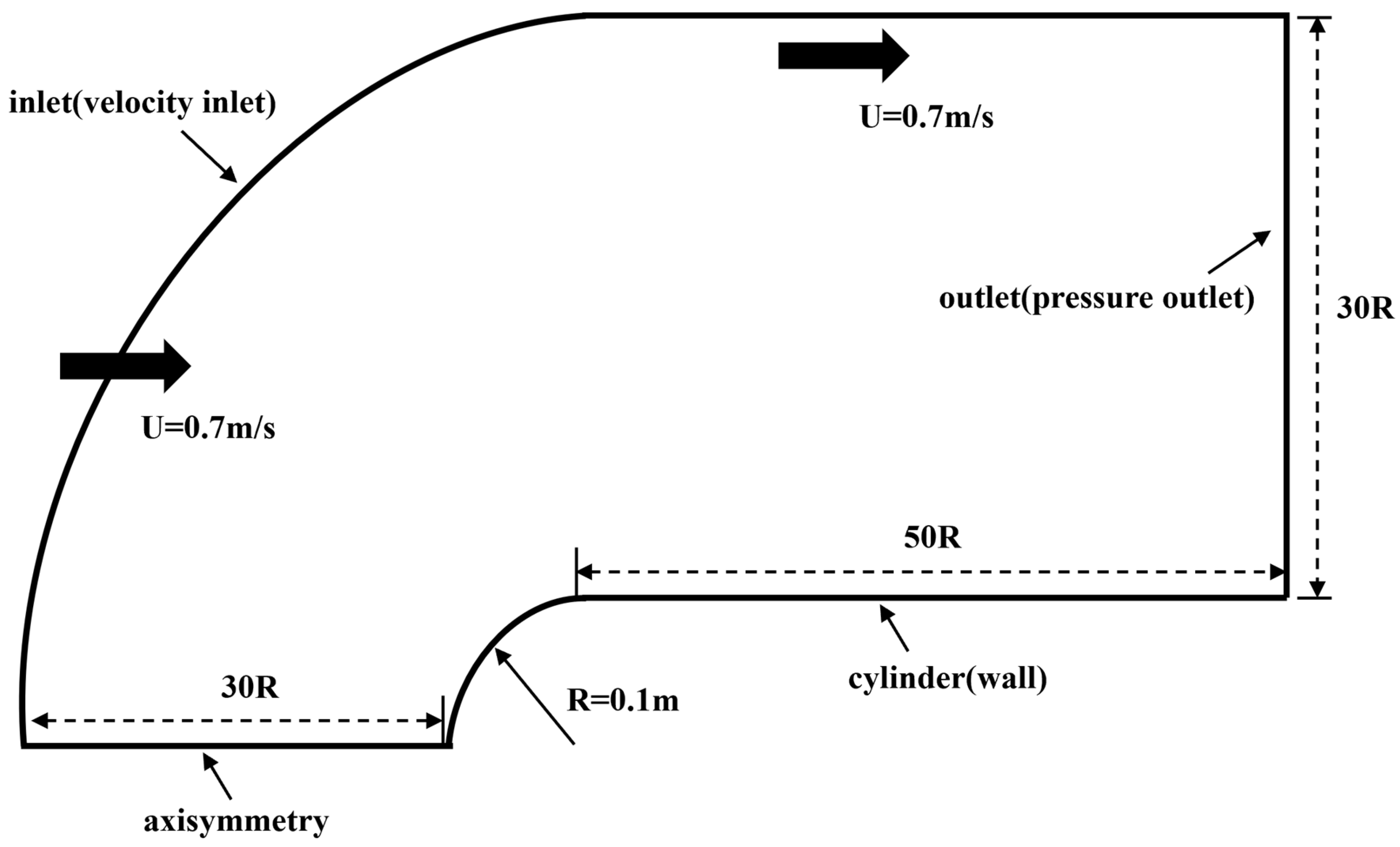
The computational domain for the numerical simulation of axisymmetric flow around a hemispherical head-form is schematically illustrated in
Figure 1. The domain is carefully structured to ensure the accurate representation of flow characteristics while mitigating potential distortions caused by boundary interactions. To achieve a balance between computational efficiency and the physical fidelity of the simulation, the domain dimensions are selected based on established best practices in numerical studies of similar flow configurations. The inlet boundary is positioned 30 times the characteristic radius
upstream of the hemispherical head to allow the incoming flow to fully develop before interacting with the model. Downstream, the outlet is placed at a distance of
to provide adequate space for wake development and to minimize numerical artifacts such as pressure wave reflections. The radial extent of the domain extends
from the centerline, ensuring that the boundary does not impose artificial confinement effects that could influence turbulence structures and cavitation behavior.
To reduce computational expenses while maintaining the accuracy of the solution, an axisymmetric boundary condition is applied along the centerline of the domain. This condition enforces the assumption that the flow is symmetric about the central axis, reducing the computational complexity compared to a full three-dimensional simulation while preserving the essential physics of the problem. The simulation is conducted under a cavitation number
of 0.3, which determines the free-stream velocity as
. This choice ensures that the computational setup accurately reproduces the expected cavitating flow conditions, facilitating direct comparisons with experimental data and theoretical predictions. At the inlet, a uniform velocity of
is prescribed, accompanied by appropriate turbulence properties such as turbulent kinetic energy
and specific dissipation rate
. These turbulence parameters are initialized using empirical formulations derived from prior studies to ensure accurate modeling of the interplay between turbulence and cavitation. At the outlet boundary, a pressure outlet condition is imposed, where the static pressure is set equal to the ambient reference pressure
, maintaining consistency with the prescribed cavitation number while minimizing artificial pressure fluctuations that could arise from numerical reflections. The lateral boundaries are placed sufficiently far from the body (typically
) to prevent artificial confinement effects that could influence the flow field. A no-slip boundary condition is applied to the solid surfaces of both the hemispherical head and the cylindrical section, enforcing zero velocity at the wall. Near-wall turbulence effects are modeled using wall functions in cases where resolving the boundary layer fully would be computationally prohibitive. The choice of near-wall treatment is based on grid resolution and turbulence model selection, ensuring an optimal balance between computational efficiency and accuracy. This domain configuration, including the inlet and outlet positions and radial extent, was selected based on validated practices established in previous studies on axisymmetric cavitating flows [
24]. The configuration ensures sufficient development of the incoming flow and prevents numerical reflections at the outlet, which are critical for achieving stable cavitation patterns. Therefore, the selected setup is not tailored to a specific case but is applicable to a broad range of similar flow conditions involving hemispherical or bluff bodies.
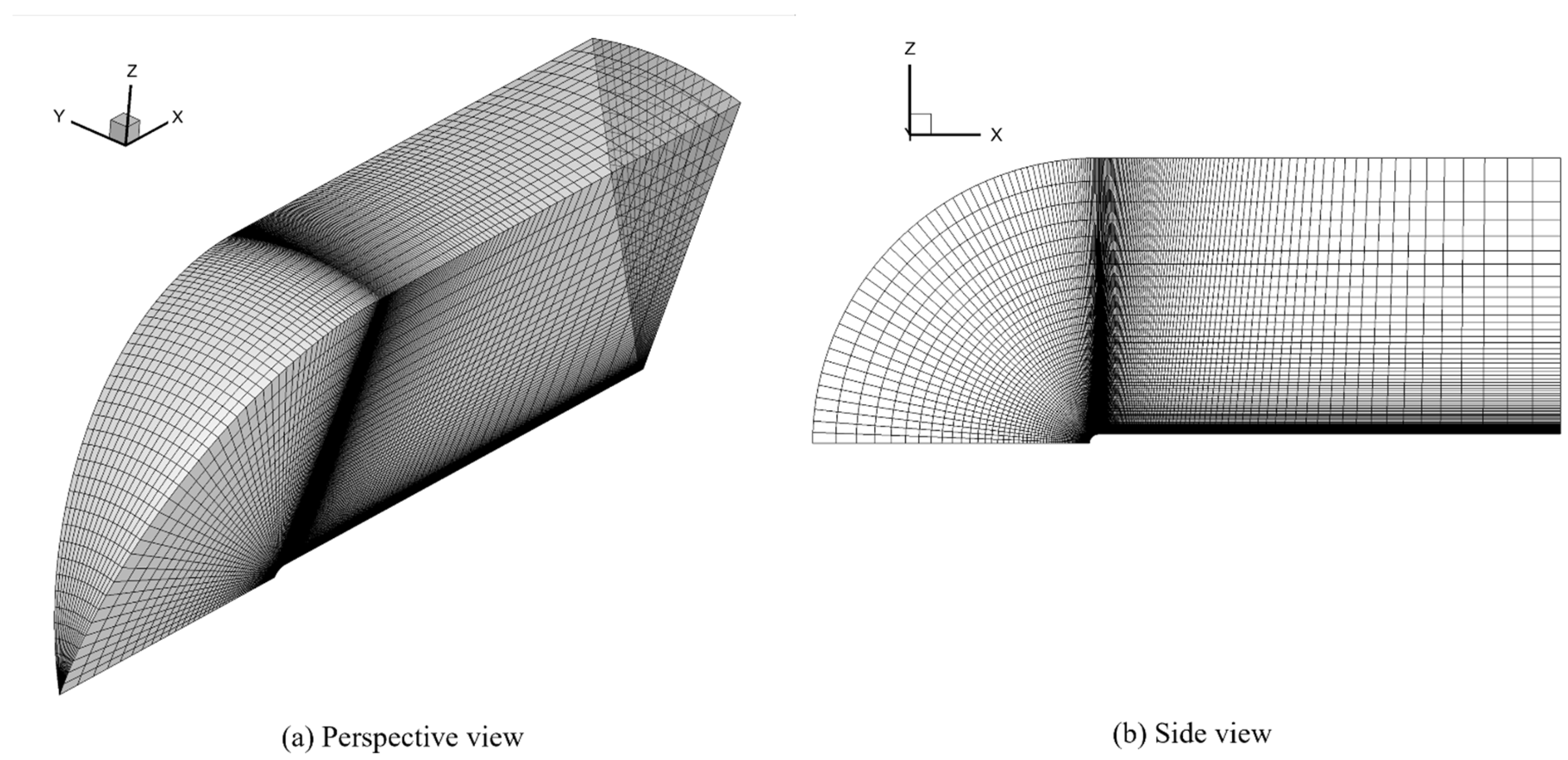
2.4. Computational Grids
Figure 2 presents the structured computational grid designed for the numerical simulation of axisymmetric cavitating flow around a hemispherical head-form body. The figure provides two views of the structured mesh: (a) a perspective view, which highlights the overall distribution and topology of the grid, and (b) a side view, which illustrates the radial and axial grid resolution. The computational grid is a body-fitted structured hexahedral mesh, carefully designed to conform to the contours of the hemispherical head-form body. This structured topology ensures high numerical accuracy by minimizing interpolation errors and improving solution stability. To accurately capture boundary layer effects and cavitation dynamics, a non-uniform grid refinement strategy is implemented. Near the wall, the grid is highly refined to resolve velocity gradients and pressure fluctuations, with the first grid layer positioned to maintain a non-dimensional wall distance
. This allows for the precise modeling of turbulence and cavitation inception.
The computational domain is discretized with
grid points along the body’s length from the inlet, while
grid points are allocated in the radial direction to capture flow structures around the hemispherical head-form. To accurately capture wake structures and cavitation effects, the domain extends downstream with
grid points from the body to the outlet. The circumferential direction is discretized using
grid points, ensuring adequate resolution of three-dimensional flow characteristics. The total number of computational cells in the structured mesh is approximately 168,000, providing sufficient refinement for capturing cavitation dynamics. A grid independence study was conducted to confirm that further refinement does not significantly alter the results of primary flow parameters such as pressure distribution, wake structure, and cavitation formation. This ensures that the grid resolution is adequate for accurately capturing flow physics without excessive computational cost. The medium grid employed in this study was selected based on a prior grid-independence study [
25] which demonstrated that key flow parameters converged with less than 2% variation between medium and fine grid resolutions.
2.5. Numerical Methods
The numerical simulations in this study were performed using OpenFOAM, employing advanced discretization techniques to enhance computational accuracy and stability. Time integration was carried out using the second-order implicit Crank–Nicolson scheme, which minimizes truncation errors and improves temporal accuracy, making it well-suited for transient flow problems. This method effectively balances numerical precision and computational cost, ensuring reliable predictions of unsteady flow characteristics.
For spatial discretization, a second-order central difference scheme was applied to compute the spatial derivatives of velocity and pressure. This scheme preserves accuracy while maintaining numerical stability, particularly in resolving complex turbulence structures. To mitigate numerical oscillations and improve solution robustness, a linear upwind divergence scheme with a limiter was implemented. This approach effectively controls numerical diffusion while maintaining the accuracy of convective transport terms, thereby ensuring stable and physically consistent results.
In the discretization of the volume fraction equation for multiphase flow, a high-resolution Total Variation Diminishing (TVD) scheme was adopted to minimize numerical dissipation. Specifically, the vanLeer scheme was applied to the convective term, which helps retain sharp fluid interfaces and prevents excessive numerical diffusion. To further enhance interface capturing accuracy, the Compressive Interface Capturing Scheme for Arbitrary Meshes (CICSAM) was utilized. This method ensures sharp and well-defined phase boundaries even in highly dynamic flow conditions, reducing interface smearing and preserving phase integrity.
For pressure–velocity coupling, the PIMPLE algorithm was employed, which integrates the Pressure Implicit with Splitting of Operators (PISO) and Semi-Implicit Method for Pressure-Linked Equations (SIMPLE) algorithms. This hybrid approach enhances numerical stability and convergence efficiency, particularly for simulations involving strong turbulence and transient multiphase interactions. The PIMPLE algorithm dynamically adjusts the number of corrector steps, improving the robustness of the solver under rapidly varying flow conditions.
By incorporating these advanced numerical techniques within the OpenFOAM framework, the computational model effectively captures complex fluid interactions, ensuring high-fidelity simulation of turbulent multiphase flows. The combination of second-order discretization schemes, specialized interface capturing methods, and an efficient pressure–velocity coupling strategy provides a well-balanced and accurate approach for solving unsteady flow problems.
To ensure solution accuracy and numerical stability, a residual-based convergence criterion was employed throughout all simulations. The iterative process continued until the residuals of all governing equations including continuity, momentum, turbulence, and vapor volume fraction were reduced below . Additionally, the number of outer corrector steps in the PIMPLE loop was set to 3 to ensure solver robustness, particularly in highly unsteady cavitating regions.
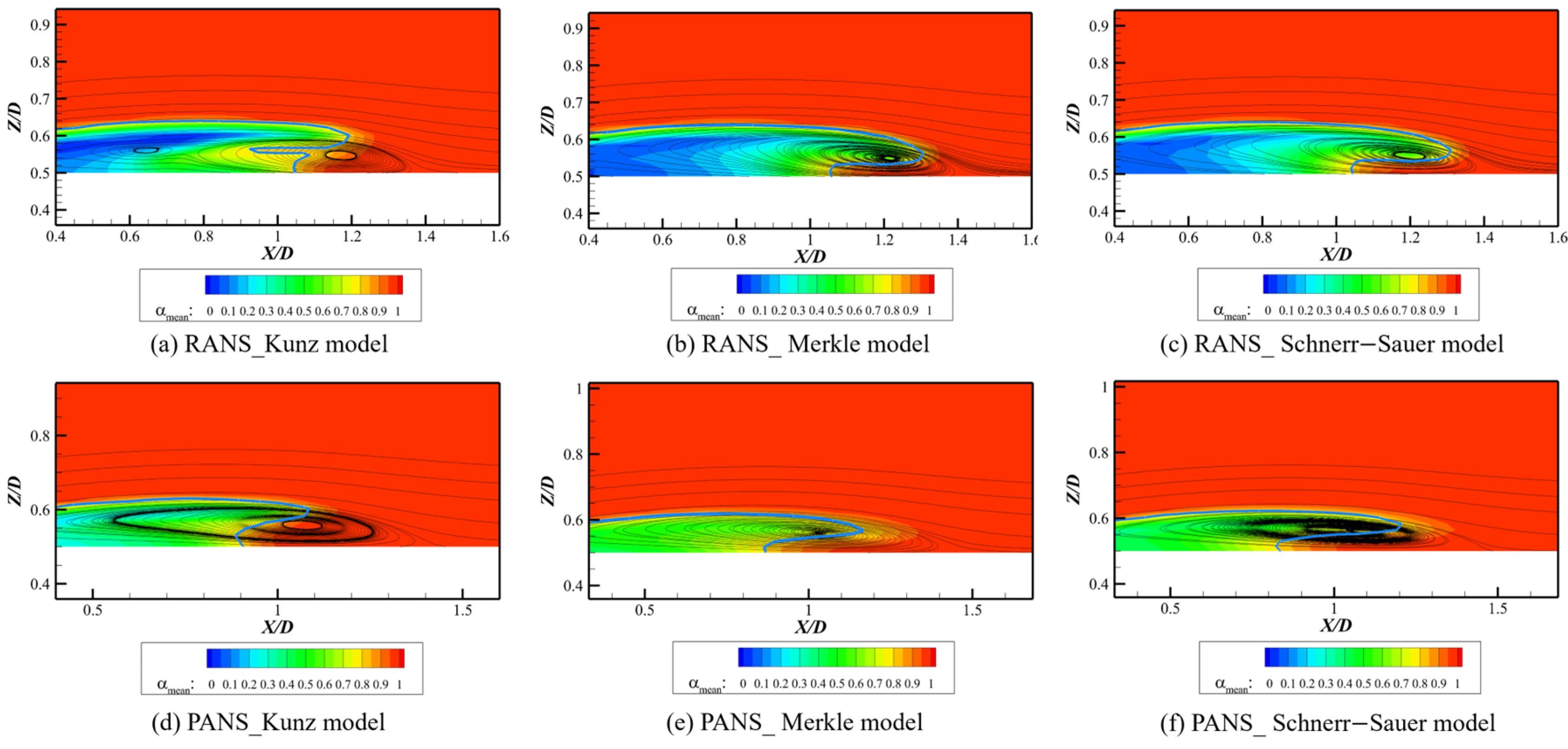
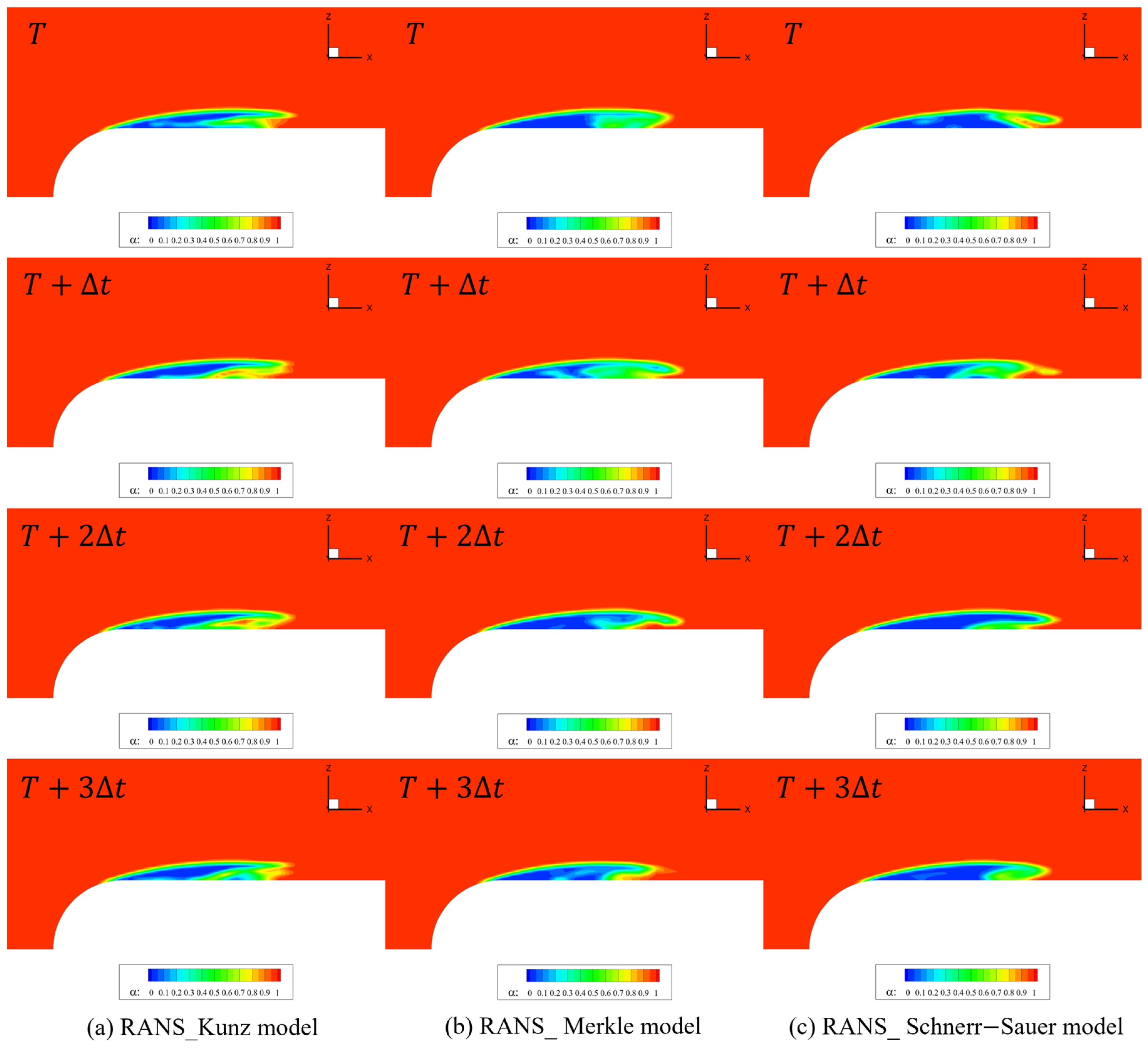
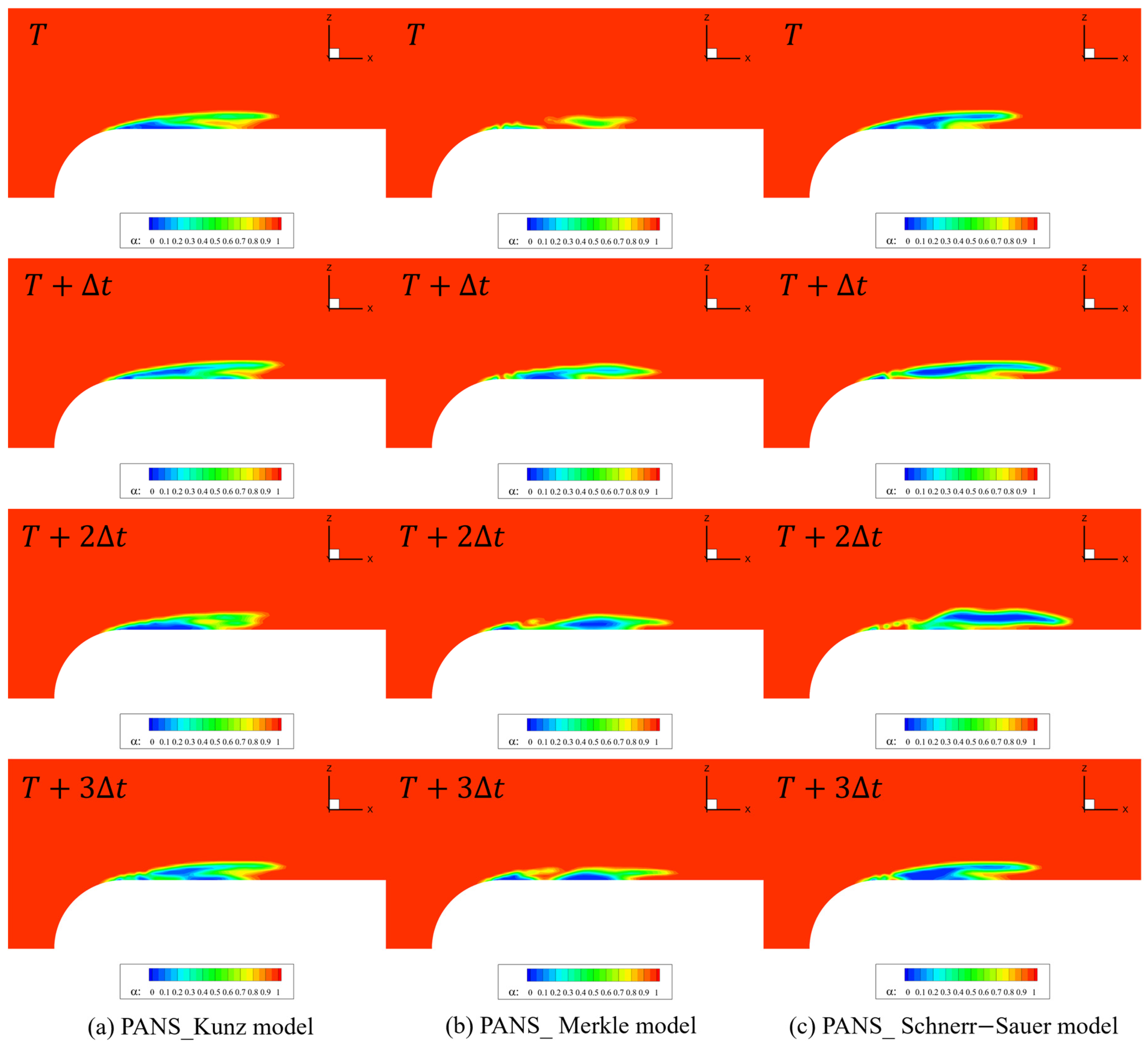
4. Summary and Conclusions
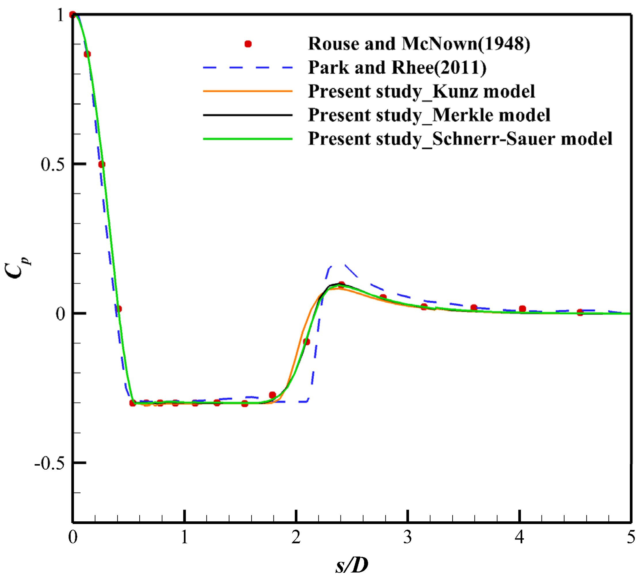
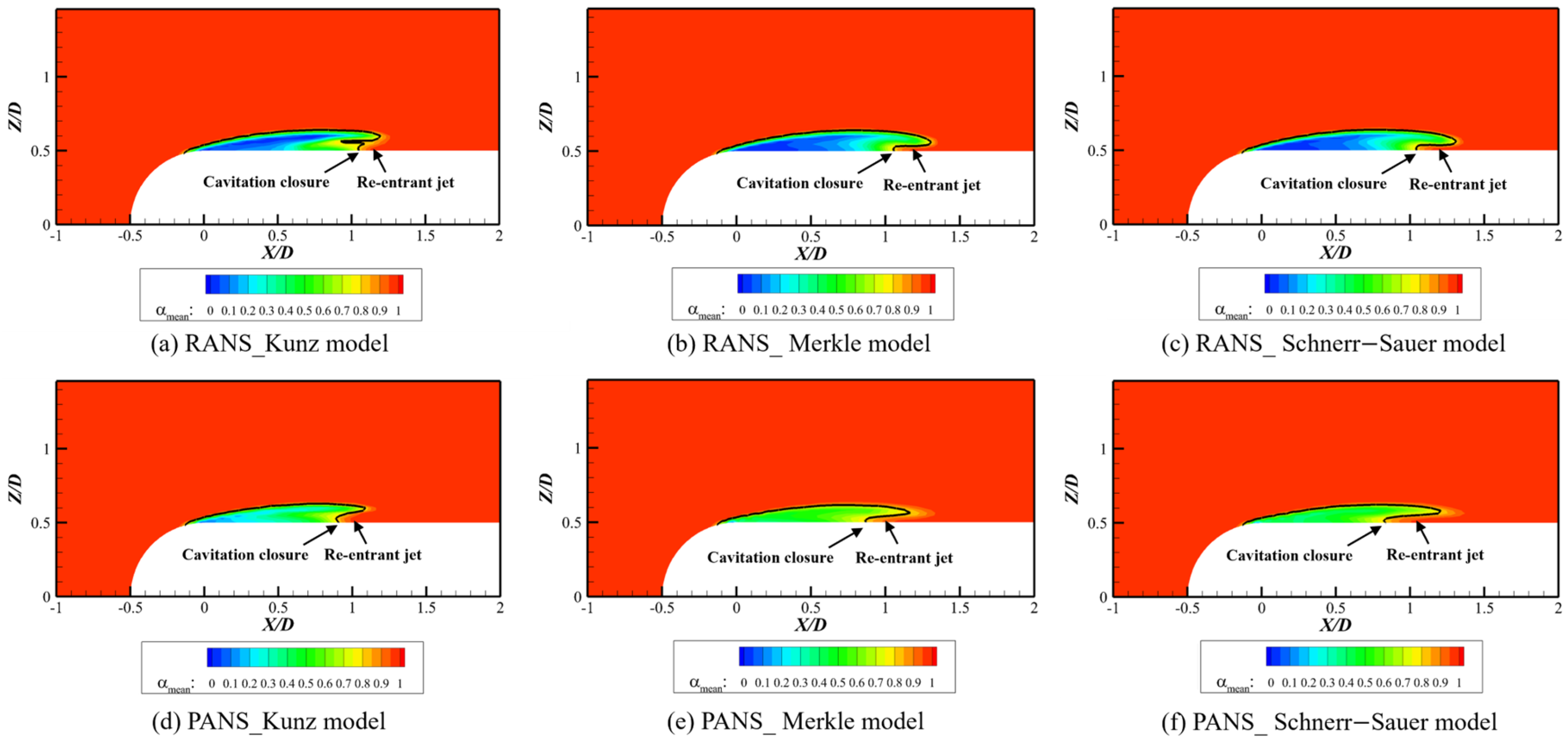
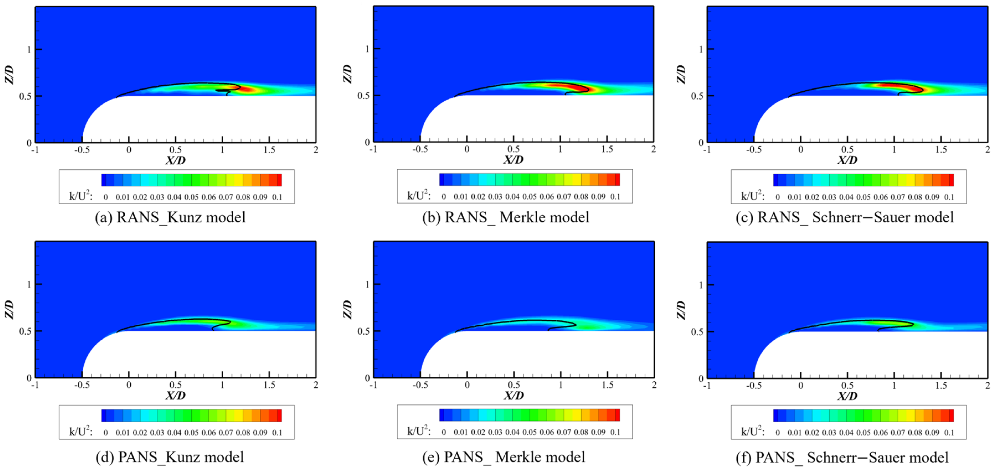
This study investigated the impact of different cavitation models (Kunz, Merkle, and Schnerr–Sauer) and turbulence modeling approaches (RANS and PANS) on the numerical prediction of cavitating flows around a hemispherical head-form body. The results demonstrated that the Schnerr–Sauer model, which incorporates bubble dynamics based on the Rayleigh–Plesset equation, provided the most accurate prediction of cavitation structures, capturing extended vapor regions and pressure fluctuations more effectively than the Merkle and Kunz models. This work contributes to the field by establishing a unified simulation framework, allowing a fair and consistent comparison across multiple cavitation and turbulence models. The identical boundary conditions and numerical setups eliminate biases, ensuring the reliability of the comparative evaluation. The Merkle model exhibited intermediate accuracy, while the Kunz model predicted a more diffused and prematurely closed cavitation region, limiting its ability to resolve transient cavitation phenomena. Turbulence modeling significantly influenced cavitation dynamics. The PANS approach consistently outperformed RANS, improving the resolution of transient cavitation structures, such as cavity shedding, re-entrant jets, and turbulence–cavitation interactions. This finding highlights the enhanced predictive accuracy of the PANS–Schnerr–Sauer model combination for transient cavitating flows, closely matching the experimental results. The PANS with Schnerr–Sauer combination provided the best agreement with experimental data, highlighting its capability in capturing unsteady cavitation behavior and turbulence interactions. An analysis of turbulence kinetic energy (TKE) confirmed that PANS reduces excessive turbulence production, resulting in a more physically accurate representation of cavitation-induced turbulence. Furthermore, by incorporating turbulence kinetic energy (TKE) analysis, the study delivers physical insights into the role of turbulence–cavitation interactions, including energy dissipation, re-entrant jet formation, and cavity deformation. This serves as a major contribution, enhancing the mechanistic understanding of unsteady cavitation dynamics.
Time-dependent analysis further revealed that RANS predicted periodic and deterministic cavitation shedding, whereas PANS captured a more continuous and irregular shedding process, leading to more accurate modeling of unsteady cavitating flows. Overall, these findings suggest that the Schnerr–Sauer model, coupled with the PANS turbulence approach, offers the highest accuracy for numerical simulations of cavitating flows. Future work should focus on extending this analysis to three-dimensional cavitating flows and higher-fidelity turbulence models such as DES and LES, as well as experimental validation using time-resolved flow measurements to further enhance model accuracy and reliability in engineering applications. Although the present study considers isothermal conditions, recent investigations such as that of Ge et al. [
15] have emphasized the importance of incorporating thermodynamic effects in cavitation modeling. Including such effects in future simulations could improve physical realism and expand the applicability of the current framework, particularly for thermally sensitive cavitating flows.


