Article

Research on the Wetland Vegetation Classification Method Based on Cross-Satellite Hyperspectral Images

1
School of Electronics and Information Engineering, Harbin Institute of Technology, Harbin 150001, China
2
North China Sea Marine Technical Support Center, Ministry of Natural Resources, Qingdao 266000, China
3
Xi’an Zhongke Xiguang Aerospace Science and Technology Co., Ltd., Xi’an 710119, China
*
Author to whom correspondence should be addressed.
J. Mar. Sci. Eng. 2025, 13(4), 801; https://doi.org/10.3390/jmse13040801
Submission received: 11 March 2025 / Revised: 15 April 2025 / Accepted: 16 April 2025 / Published: 17 April 2025

Abstract

:
In recent years, the global commercial aerospace industry has flourished, witnessing a rapid surge in customized satellite services. Deep learning has emerged as a pivotal tool for accurately identifying wetland vegetation. However, hyperspectral remote sensing images are often plagued by varying degrees of noise during acquisition, leading to subtle differences in spectral responses. Currently, vegetation classification models are tailored specifically for each hyperspectral sensor, making it challenging to generalize a model designed for one sensor to others. Furthermore, discrepancies in data distribution between training and test sets result in a notable decline in model performance, impeding model sharing across satellite hyperspectral sensors and hindering the interpretation of wetland scenes. Domain adaptation methods leveraging Generative Adversarial Networks (GANs) have been extensively researched and applied in the realm of cross-sensor land feature classification. Nevertheless, these data-level cross-domain classification strategies typically focus on band selection or alignment using relatively similar data to address image differences, without addressing spectral variability or incorporating pseudo-labels to enhance classification accuracy. Noise changes aggravate the distribution characteristics and model differences of vegetation in classification tasks. This has a negative impact on subsequent classification accuracy. To alleviate these problems, we have designed a linear unbiased stochastic network classification framework based on adversarial learning. The framework employs a style randomization algorithm to simulate spectral drift. It generates simulated images to enhance the model’s generalization ability. Supervised contrastive learning is utilized to prevent redundant learning of the same training images. Domain discrimination and domain-invariant characteristics are considered. We optimize the generator and discriminator using inter-class and intra-class contrast loss functions. The dual regularization training method is adopted, and non-redundant expansion is realized. It achieves similarity and addresses offsets. This method minimizes computational cost. Cross-sensor classification experiments were conducted, with comparative tests performed on a self-made wetland dataset. This method demonstrates significant advantages in wetland vegetation classification. According to the visualization results, our classification strategy can be used for cross-domain vegetation classification in coastal wetlands. It can also be applied to other small-satellite hyperspectral images and cross-satellite multispectral data, reducing on-site sampling costs and proving cost-effective.

1. Introduction

In recent years, the global commercial aerospace industry has thrived, with numerous countries offering customized services for small satellites tailored to meet practical needs. Hyperspectral remote sensing is becoming increasingly widely used in vegetation ecological monitoring [1]. Hyperspectral remote sensing has driven remote sensing applications towards a more precise and accurate direction [2]. However, due to factors inherent to hyperspectral imaging systems and external imaging environmental conditions (such as sensor technology, atmospheric interference, sampling distance and angle, etc.), hyperspectral remote sensing images are subject to varying degrees of noise interference during acquisition [3], resulting in slightly different spectral responses. Currently, the vegetation classification models that have been constructed are customized for each specific hyperspectral sensor. Due to these spectral differences, it is often difficult to convert a model designed for one sensor into a general model [4]. This is a long-standing problem in deep learning, where the distribution differences between the training and test sets significantly degrade model performance [5]. In cross-domain classification tasks, a large generalization error and poor interpretability hinder model sharing among satellite hyperspectral sensors and the interpretation of wetland scenes [6]. Conducting on-site surveys is an effective means to enhance model performance. However, acquiring ground samples typically demands professional expertise and considerable manpower [7,8]. This is particularly evident in coastal wetland environments, which are intricate and host a diverse array of vegetation types. Most areas are difficult to access, making it challenging to obtain comprehensive training data, which limits the scale and diversity of training data for classification models [9].
Domain adaptation methods based on Generative Adversarial Networks (GANs) [10,11] are widely studied and applied in the field of cross-sensor land feature classification. They consist of a network architecture composed of a generator and a discriminator. The goal of the generator is to generate realistic samples, while the discriminator aims to determine whether a given sample is real or generated. The adversarial optimization objectives of the two enable the generator to learn the sample distribution of the training samples well. They are mainly used to address the domain shift problem between remote sensing images obtained from different geographical regions or different sensors, thereby improving the generalization ability and accuracy of classification models in new domains [12]. Currently, researchers have proposed various GAN-based domain adaptation methods to improve the effect of classification.
The neural network domain adversarial training proposed by Ganin et al. [13] embeds a gradient reversal layer in the backpropagation training for feature alignment, achieving domain-level feature alignment. However, due to the lack of discriminative training, the class information of the target domain data is ignored, which may lead to the side effect of reduced feature discrimination. The conditional adversarial domain adaptation model proposed by Long et al. [14] constructs a conditional domain discriminator based on the cross-variance of domain-specific feature representations and classifier predictions, that is, determining the identification domain result based on the uncertainty of classifier predictions. The adversarial discriminative domain adaptation model proposed by Tzeng et al. [15] combines discriminative modeling, joint weight sharing, and generative adversarial loss. It first learns a discriminative representation using labels in the source domain and then uses a separate encoder to map target data to the same space using asymmetric mappings learned through domain adversarial loss.
Meanwhile, scholars have also constructed some new models based on GANs, such as Cycle GAN [16], which maintains cycle consistency through generators in both directions, ensuring that generated images can be restored to their original state after inverse translation. This method helps maintain the semantic information of the images unchanged and has significant advantages in cross-domain classification tasks with large differences in image resolution or across different scenes. However, the generator may still be unable to generate diverse samples in the same classification scenario. Adversarial Discriminative Domain Adaptation (ADDA) freely adjusts the parameters of each layer during training without being constrained by fixed weights. This flexibility helps the model better adapt to the distribution differences between the source and target domains, but it is very sensitive to the selection of hyperparameters, and different hyperparameter settings may lead to significant differences in training results [15,17]. The Dual GAN bidirectional transformation mechanism not only enhances the generalization ability of the model but also helps improve the quality and consistency of images in the source and target domains. The cycle consistency constraint may have inherent ambiguity for geometric transformations, and image content corruption may sometimes be observed during the transformation process [18]. Domain adversarial neural network (DANN) is a method that contrasts with classical approaches, where representation and classifier learning occur at different stages. DANN learns a representation that is discriminative and invariant to shifts in a single dataset during the learning phase [13].
Li established a transfer learning network based on TCGAN and introduced a “generation transfer” collaborative training strategy based on expectation maximization, which realized the parallel update of generation network and transfer network parameters [19]. Some scholars also proposed a new GAN generated image detection framework by estimating the similarity of artifacts, expanding the differences between different categories (GAN-generated or original images), and improving the intra-class compactness of different domains (source attributes) in the same category [20]. Ma proposed a mutually enhanced attention transformer (MBATrans) to capture the cross-domain dependency of semantic feature representation to enhance the generalization of the GAN (MBATA-GAN) architecture [21]. Xu proposed a self-ensembling generative adversarial network (SE-GAN) exploiting cross-domain data for semantic segmentation. A teacher network and a student network constitute a self-ensembling model for generating semantic segmentation maps, which, together with a discriminator, forms a GAN [22]. Researchers improved the generator to enhance the stability and generalization of the model.
In the application of cross-domain remote sensing classification tasks, existing cross-domain remote sensing scene interpretation methods generally reduce the domain differences between the source domain and the target domain from three different levels: data, features, and models, thereby enabling the model trained on the source domain to generalize better to the target domain [23]. Mateo-García proposed a domain adaptation framework based on cyclic consistent generative adversarial networks to train a transformation model in an unpaired manner, aiming to reduce the statistical differences between two multispectral sensor images and thus improve the transfer performance of the learned model [6]. For hyperspectral data sources, most research results are based on domain adaptation techniques for homogeneous hyperspectral data, where images are acquired by the same sensor and contain the same spatial and spectral resolutions. Yu proposed a hyperspectral UDA method based on content alignment to achieve feature alignment, reducing content differences through an adversarial framework to enhance the representation of invariant features [24]. Ma et al. [25] proposed an adversarial-based domain adaptation method for unsupervised cross-dataset hyperspectral image perception, which enforces global alignment between the source and target domains and uses multiple classifiers to establish a discriminator, driving the learning of target samples in an adversarial manner. Wang introduced a spectral learning branch in the generator to reduce the impact of noise on pseudo-randomness in the data cube and employed a two-stage alignment to help the model eliminate domain bias [26].
A few scholars have also challenged the research on cross-sensor classification strategies. The source and target domains captured by different sensors have different spectral and spatial resolutions, leading to the key issue of non-equivalent data representation across domains. Both data-level alignment and feature-level alignment start from the data of the target and source domains, aiming to eliminate data differences through data mapping, thereby improving robustness without changing the model [25]. Mesay Belete proposed an adversarial domain adaptation framework based on DANN, combining representation learning, domain adaptation, and classifier learning in a single training process. By minimizing domain differences using the Wasserstein metric, it addresses cross-domain classification of hyperspectral images from sensors with different channel counts [27]. Indrajit Kalita proposed a cross-sensor domain adaptation strategy that uses deep neural networks to explore solutions in cross-sensor environments, combining land cover classification (LCC) models with active learning (AL) strategies [28]. The sample strategy balances the number of cross-sensor data samples in terms of feature size and availability and merges target samples through labeled sources and “maximum information” to train classifiers, but it does not consider the impact of spectral variability on classification accuracy [29]. Amir Mahmoudi proposed an end-to-end network, namely Generative Adversarial Network Heterogeneous Domain Adaptation (GANHDA), which combines dual classifiers, variational autoencoders, and graph regularization to transfer high-level concepts from the source domain to different dimensions and minimally labeled knowledge target domains, aiming to improve classification performance, but it requires the addition of pseudo-labels to surpass accuracy limitations [30].
However, the cross-domain classification strategy based on the data level often selects relatively similar data for band selection or band alignment in addressing image differences, without focusing on spectral variability or adding pseudo-labels to improve classification accuracy. Due to Gaussian noise in the photoelectric conversion process of hyperspectral detectors and spectral differences caused by atmospheric noise, Gaussian noise is randomly distributed across various bands in hyperspectral images, with different noise intensities in different bands [31]. Atmospheric noise leads to significant attenuation of radiation signals in certain spectral bands, resulting in extremely low signal-to-noise ratios in some bands. Especially in vegetation classification tasks, the differences in noise further increase the distribution characteristics and model discrepancies of vegetation, affecting subsequent classification accuracy [32].
In our research work, we construct a classification model, train it on one satellite, and test the classification task on another satellite. As a typical representative of cross-sensor classification research, we focus on the Gaofen-5 (GF-5) satellite [33] and the Xiamen Technology-1 (XG-003) satellite [34] in this paper. GF-5 has a revisiting period of 5 days, while XG-003 is a customized urban service satellite that utilizes a miniaturized and low-cost small satellite platform. It operates in a sun-synchronous orbit with an orbital altitude of approximately 530 km, acquiring continuous time-series data and global coverage. Its revisiting period is generally 1 to 2 days. Compared to GF-5, XG-3 differs in terms of shooting angle, spatial resolution, spectral resolution, and other aspects.
We introduce a linear unbiased random network classification framework tailored for wetland scenarios. By generating style-randomized spectral images within the generator, the simulated images encompass spatial-spectral features with spectral shifts relative to the training images. This approach mitigates spectral offsets arising from different sensors and diminishes the reliance on field-labeled data in wetland scenarios. Furthermore, to comprehensively extract both global and local spatial-spectral features, we employ a dual-branch model. This model comprises a multi-scale spectral feature extraction module and a dual-branch module based on a three-dimensional Convolutional Neural Network (CNN) and a Transformer encoder. This setup achieves the generalization of the vegetation classification model, enhancing the accuracy and reliability of wetland remote sensing image interpretation, especially in scenarios with limited data.
In the Section 2 of the article, we provide a detailed introduction to the proposed classification framework, methods, and experimental GF-5 and XG-003 data. The Section 3 presents the results and discussion of the training and testing experiments, while the Section 4 summarizes and presents prospects for the experiments and the article.

2. Method and Data

2.1. Method

We utilize a linear unbiased randomized network to address the issue of satellite hyperspectral image classification across satellite sensors (see Figure 1). The network comprises a generator for data generation and a discriminator for learning domain-invariant representations. During the training phase, the generator and discriminator mutually optimize each other, ultimately training a discriminator with generalization capability. In the testing phase, features are extracted by the generator and then directly classified by the discriminator. To achieve generalization of the network, the network incorporates a generator featuring linear response and style randomization, which can generate simulated images (the simulated image is generated from the segmented image). It can generate simulated images that have a certain degree of similarity to the training images but also exhibit spectral shifts, thereby enhancing generation efficiency and reliability. Furthermore, the dual adversarial regularization training method of the generator and discriminator achieves redundancy-free expansion, ensuring similarity and offset between training images and simulated images at a lower computational cost.
First, the hyperspectral image is segmented into image blocks. For each super pixel of the segmented hyperspectral image, a three-dimensional data cube with the shape of p × p × S is intercepted from the super pixel as the center as a sample, which is then sent to the multi-scale spectral feature extraction module to extract spectral features, obtaining spectral features of different scales that are connected as feature maps. Through the joint extraction and fusion of line space features and spectral features of the dual-branch CNN Transformer module, Global average pooling is utilized to flatten the feature map into a single vector, which is then fed forward to the linear layer to obtain the classification probability. Subsequently, the loss function is calculated, and backpropagation is performed to update the model parameters. Specifically, the gradients of all parameters are cleared, the gradient of the loss function with respect to the model parameters is calculated, and the model parameters are updated based on the calculated gradient.
Through this process, the model continuously adjusts parameters in multiple iterations to minimize the loss function and finally reaches the convergence state. After training, a patch is built from the hyperspectral image and fed to the proposed network to obtain the classification results using the dual-branch CNN-Transformer (DBCT) [35].

2.1.1. Generator

The generator is an asymmetric, masked autoencoder structure that takes into account spectral diversity. In the generator, the pseudo-data generated from training images are referred to as simulated images. The generator generates simulated images by reconstructing data from the learned domain-discriminative representation, ensuring that the simulated images incorporate spatial-spectral features with spectral shifts relative to the training images.
The encoder encompasses linear resampling and feature extraction utilizing 3D convolution. Following super-pixel segmentation, the hyperspectral image is segmented into super-pixel blocks of comparable size, and the largest inscribed rectangle is selected for processing. Pixels within each super-pixel share the same label, thereby considering each super-pixel as a distinct sample rather than each individual pixel. The resulting hyperspectral image blocks undergo spectral channel scaling and spatial-spectral feature extraction via 1 × 1 2D convolution and 3 × 3 × 3 3D convolution, ultimately yielding image block features z.
Unbiased Randomization: Calculate the mean and variance of the image patch features z, generate a style image x, and then randomly generate another style image y. Through adaptive learning of affine transformation parameters, transfer the style of x to the previous image:
AdaIN ( x , y ) = σ ( y ) ( x μ ( x ) σ ( x ) ) + μ ( y )
μ and σ represent the mean and variance of the image block, respectively.
AdaIN (Adaptive Instance Normalization): The core of the method lies in the adaptive instance normalization layer, which aligns the mean and variance of content features (features of source domain images) with those of style features (features of target domain images). The fundamental idea is to normalize features from two perspectives: instance normalization and adaptive adjustment.
Instance normalization involves performing normalization separately on each sample (usually one sample per batch). Given a feature map x with shape C × H × W , where C represents the number of channels, H and W represent the height and width, respectively, the formula for instance normalization is as follows:
μ ( x ) = 1 H W i , j x c i j , σ 2 ( x ) = 1 H W i , j x c i j μ ( x ) 2
μ x is the mean value on channel C, and σ 2 ( x ) is the variance. The normalized feature map x norm is
x n o r m = x μ ( x ) σ 2 ( x ) + ϵ
where ϵ is a very small positive number used to avoid division by zero.
Adaptive adjustment refers to adjusting the normalized feature map using scale and offset parameters obtained through learning. The target domain image is input into a pre-trained neural network (such as VGG), and high-level features are extracted through several layers of the network. Statistical features, including the mean and covariance matrix, are calculated from the feature maps extracted from these layers. These statistical features reflect the stylistic characteristics of the style image. These statistical features are then concatenated into a vector y, serving as the style vector. The formula for adaptive adjustment is as follows:
A d a I N = γ x n o r m + β
where γ and β are the scale and offset parameters calculated from the style vector y, which are learned from the style vector y through a fully connected network structure.
Decoder: The decoding process is the inverse of the encoding process, consisting of deconvolution. Through deconvolution calculations, the image block size is restored through upsampling.
To optimize the generator, the following loss function L a d v is used as a constraint for generating simulated images:
L a d v = c i = 0 n c 1 | P c ( i ) | p N c ( i ) log e x p ( S ( z i , z p + ) / τ ) a N c ( i ) e x p ( S ( z i , z n ) / τ )
By designating class C as positive samples and all other classes as negative samples, continuously narrowing the intra-class distance while widening the inter-class distance facilitates the generation of effective simulated images through intra-class contrastive learning.

2.1.2. Double Branch Discriminator

The discriminator consists of a classification projection, a feature projection, and a feature extractor. It is primarily utilized for feature extraction and classification of both training images and simulated images. In the training phase, the discriminator is used to classify the samples of training images, analog images, and mixed images (the mixed image is the weighted result of training image and analog image), and then the prediction result and feature projection are generated. The generator and discriminator carry out contrastive confrontation learning by generating analog image samples and learning invariant representations.
In order to fully extract global and local spatial-spectral features, the feature extractor uses a dual-branch model. The model is mainly composed of two parts: the multi-scale spectral feature extraction module and the dual-branch module based on three-dimensional convolutional neural network (CNN) and Transformer encoder. In order to fully extract spectral features, a multi-scale spectral feature extraction module is proposed. The multi-scale spectral feature extraction module enables the model to obtain different receptive fields to extract spectral features at different scales, which enriches the extracted features and improves the performance of the model. Based on the original Transformer encoder, an improved Transformer encoder module through convolution operations is designed, and a convolutional spectral projection unit and a convolutional multi-head self-attention unit are proposed to extract spatial and global spectral features. The module can fully integrate spatial and local-global spectral features while maintaining low computational complexity.
Multi-scale spectral feature extraction module: This module extracts the features of the original training image, the simulated image output by the generator, and the mixed image obtained by the linear combination of the two. First, a 1 × 1 × 7 3D convolution layer is employed for dimensionality reduction. Then, it is divided into four sections along the channel dimension, each representing features of different scales. Three-dimensional depth-wise separable convolutions with varying kernel sizes are applied to each section of features. Each 3D depth-wise separable convolution is followed by a ReLU function to extract spectral features of different scales. Finally, the multi-scale features are concatenated along the channel dimension to obtain the feature map.
Based on 3D CNN and Transformer encoder module: This module carries out joint extraction of spatial and spectral features. The two branches are CNN and Transformer encoder, improved by convolution operations. The Transformer encoder branch improved by convolution operations is composed of a convolution layer, a convolution projection layer, and a convolution multi-layer perceptron. Using the long-distance dependence modeling ability of the Transformer, the convolution multi-head self-attention mechanism is applied to each spectral band, which can capture better global spectral features from multiple spectral bands. Then, the global space spectrum characteristics of the Transformer encoder are output through the 3 × 3 × 1 3D convolution layer of one channel. The CNN branch is relatively simple. It is calculated through 16 channels of 3 × 3 × 3 3D depth-separable convolution and 1 × 1 × 1 3D point-by-point convolution, and then through the batch standardization layer, post ReLU function, output space, and local spectral characteristics.
Classification projection uses Softmax function to obtain the classification result of each super-pixel. The feature projection is used to calculate the loss function, and the following loss function L c o n is used as the constraint of the discriminator to optimize the discriminator:
L c o n = t = 0 N 1 | P ( i ) | p P ( i ) log e x p ( S ( z i , z p + ) / τ ) a N ( i ) e x p ( S ( z i , z n ) / τ )
Using training images as positive samples and simulated images as negative samples, we increase the similarity between the samples and training images while decreasing it with simulated images, enabling the discriminator to learn a domain-invariant representation.

2.2. Data

The classification experiment presented in this paper is divided into two parts. Initially, we aim to assess classification accuracy on a public dataset. Then, we apply the classification method to practical scenarios in the Yellow River Estuary Wetland of China, utilizing two different hyperspectral satellite data sources. Detailed descriptions of the dataset area and technical parameters are provided below.

2.2.1. Public Dataset

The Pavia dataset comprises scenes from the Pavia Center (PC) and Pavia University (PU), consisting of airborne reflectance spectroscopy data collected by the ROSIS-03 sensor (Reflective Optics Spectrographic Imaging System, Germany) over Pavia, Italy. It provides insights into various Pavia landscapes with spectral coverage ranging from 430 to 860 nm. The PU subset has a spatial resolution of 610 × 340 pixels in 103 spectral bands, while the PC subset has a larger spatial footprint of 1096 × 715 pixels with 102 spectral bands. The two datasets have seven common categories. The dataset covers various surface feature types of urban and natural environments, such as buildings, roads, vegetation, etc., and is suitable for multi-category classification tasks. The number of samples in the dataset is shown in Table 1.
The Shanghai-Hangzhou dataset is from EO-1 satellite images, capturing the spectral characteristics of Shanghai and Hangzhou, with the spectral range extending from 357 nm to 2567 nm. The Shanghai scene spans 1600 × 230 pixels, and the Hangzhou scene spans 590 × 230 pixels. Both scenes have 198 bands and 3 categories. The number of samples in the dataset is shown in Table 2.

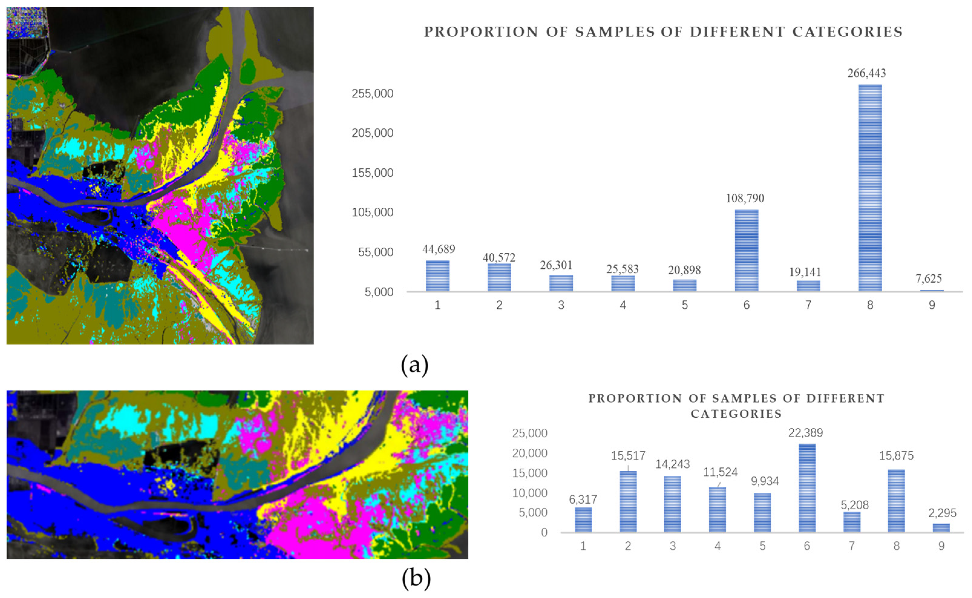
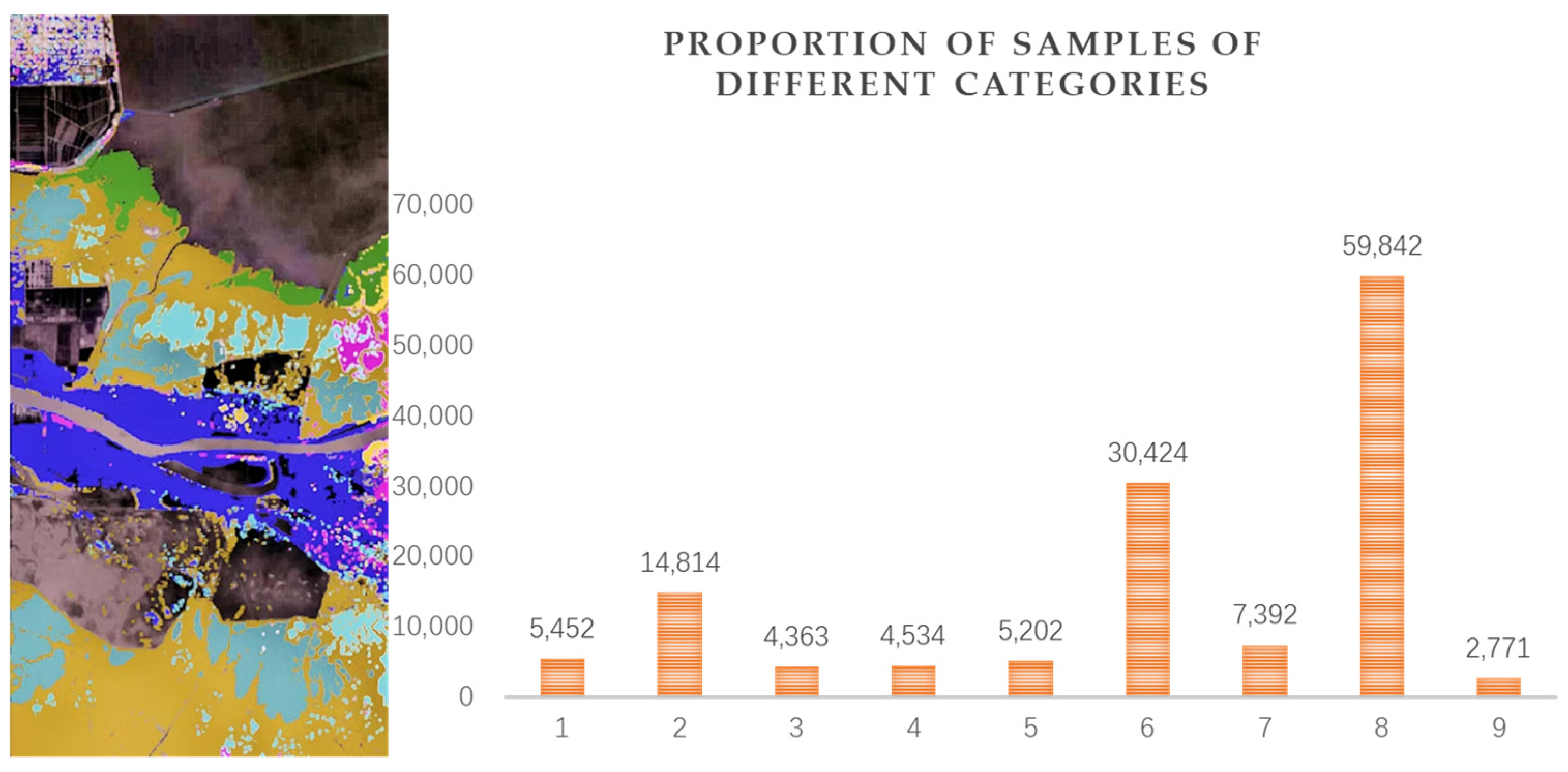
2.2.2. Hyperspectral Satellite Data of Yellow River Estuary Wetland

The experiment was conducted using a self-made dataset, with the GF-5 hyperspectral image serving as the source domain and the XG-003 hyperspectral image serving as the target domain, for the classification of ground objects and typical vegetation. Detailed technical indicators are provided in Table 3 below.
In this experiment, some typical vegetation distribution areas in the Yellow River Delta Nature Reserve were selected. In the nature reserve, Suaeda salsa is mixed with Tamarix chinensis Lour, Phragmites australis, Spartina alterniflora, and other plants, and most of them are short and sparsely distributed [36]. Spartina alterniflora, as an alien species, lacks natural enemies, has strong reproductive capacity, and invades a large number of ecological niches, which has seriously threatened the survival of local species in the Yellow River Delta [37]. Therefore, Suaeda salsa, Spartina alterniflora, Phragmites communis, and Tamarix chinensis Lour were identified in the hyperspectral image classification task.
Since the two satellites have different bands of hyperspectral images, we first compared the band ranges of the two satellites, aligned the bands of the two satellite sensors, and screened 98 wavebands for alignment between 430 and 880 nm. The corresponding labels of the training data include Spartina alterniflora, Phragmites australis, Tamarix chinensis Lour, Suaeda salsa, Tidal Beach, Water Body, and nine other categories (see Table 4). The GF-5 truth map was downsampled according to the image resolution, and the resolution was reduced from 30 m to 40 m. A total of 763 × 734 pixels were obtained as training data, considering that model learning tends to dominate classes, and its ability to recognize minority classes is weakened, which is manifested by decision boundary deviation, insufficient feature learning, traditional evaluation indicators such as accuracy distortion, and potential overfitting of most classes. In subsequent experiments, the training image GF-5 will be trimmed to balance the distribution of categories, 196 × 527 pixels were obtained as training data. The distribution of category samples is shown in Figure 2 to ensure that the model has good comprehensive classification performance and generalization ability.
XG-003, the image size is 557 × 242, as shown in Figure 3. The image contains nine types of typical vegetation across the Yellow River Estuary and representative surface features of the Yellow River Estuary Wetland.

2.3. Other

This experiment is based on the Windows 10 operating system, trained and validated on the NVIDIA GeForce RTX 4090 (GPU), and optimized using the Adam optimizer. The size of each batch of samples is 32. The Epoch_avr is 1.1454.

3. Experimental Results and Analysis

Firstly, we conducted unsupervised classification experiments on the Yellow River Estuary wetland image, utilizing GF-5 hyperspectral images for training and XG-003 hyperspectral images for testing, using OA (Overall Accuracy) and AA (Average Accuracy) as quantitative evaluation metrics. However, due to the significant time gap between the acquisition of the two images, significant changes in the ground feature scene, and the impact of tidal variations and ground feature obstructions during image acquisition, the experimental results were not ideal. Therefore, we conducted a supervised classification experiment, training 70% of GF-5, testing 30% of GF-5, training 70% of XG-003, and testing 30% of XG-003. The structure of the feature extractor was learned during this experiment. Then, the idea of semi-supervised cross-domain classification is proposed, trained using the entire training image dataset and 70% of the test image dataset, and tested using the remaining 30% of the test image dataset. The experiment was conducted on two public datasets, and the model was also applied to a self-created Yellow River Estuary wetland dataset. Compared to the supervised classification experiment, this experiment enhanced the training and learning process for the test images, resulting in an improvement in the average classification accuracy.

3.1. Unsupervised Cross-Domain Hyperspectral Object Classification Experiment

Based on previous cross-domain hyperspectral image classification methods, we utilize GF-5 images as the source domain and XG-003 images as the target domain for cross-domain classification tasks. SDE net [38] can effectively capture the spatial distribution characteristics of wetlands, but it requires an excessive amount of labeled data for training. LLU net [39] can effectively capture the details of wetland features, particularly for vegetation and water boundaries, making it suitable for small samples. The test was conducted on a self-created coastal wetland dataset, which was influenced by water bodies and other environmental factors, coupled with the complex intermingling of vegetation. Consequently, relying solely on the source domain images for training resulted in a model with limited generalization capabilities. The classification results are presented in Table 5 and Table 6 and Figure 4. The results indicate limited applicability in field conditions without labeled data.

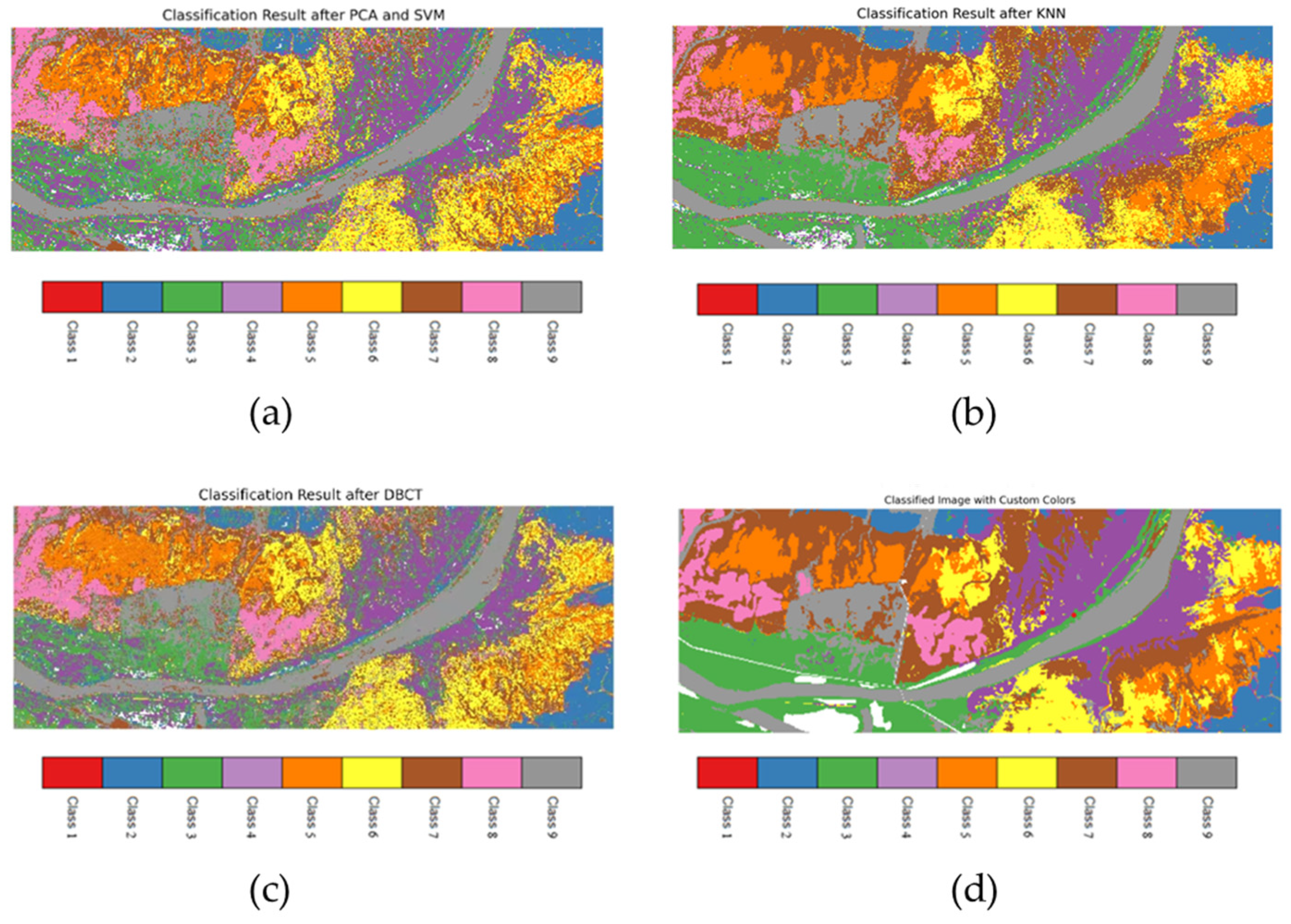
3.2. Supervised Cross-Domain Hyperspectral Object Classification Experiment

After the initial model learning, the structure of the feature extractor is determined. Simultaneously, the support vector machine (SVM) [40] as a representative of classic algorithms was chosen for comparative experiments; since the data contains a small amount of labeled data and a large amount of unlabeled data, the k-nearest neighbor algorithm (K-NN) [41] can better predict the labels of unlabeled data points.
Due to the poor generalization performance of models trained solely on source domain images, this experiment initially employed SVM, K-NN, and DBCT to train and test a classification framework on GF-5 and XG-003 images. The results, as shown in Figure 5 and Table 7, indicate that for GF-5 images, the DBCT exhibits the best classification performance, followed by the K-NN. All three methods achieve the highest classification accuracy for Class 1, Spartina alterniflora, and the lowest for Class 5, Phragmites australis, on the Tidal Flats. This is primarily because the spectral characteristics of Class 1 Spartina alterniflora samples are highly distinguishable from other classes in the training data, making it easier for the model to learn these features. However, the spectral characteristics of Class 5 Phragmites australis on the Tidal Flats samples are similar or overlap with those of Class 2 Phragmites australis, and the spatial differences are more pronounced, making it difficult for the model to accurately distinguish between them, leading to poor classification performance. Secondly, the classification performance is poor for Class 9, Other, due to the small number of samples in this class. During training, the model tends to favor the majority class, resulting in poor classification performance for the minority class.
The XG-003 image classification is also affected by the uneven distribution of samples. As shown in Table 8 and Figure 6, the number of samples of the Class 1, Class 3, Class 4, and Class 5 categories is far less than that of other categories, so the classification accuracy of these four categories is low. This problem is more obvious in the SVM, as when there is a significant disparity in the number of samples between different categories, SVM tends to maximize the overall classification margin. This approach may result in less precise classification boundaries for minority samples, as they contribute less to maximizing the margin. Consequently, the boundaries of minority classes may be dominated by those of the majority classes, thereby diminishing the model’s predictive ability for minority classes. The K-NN has better classification accuracy for each category because it is a learning method based on instances. It does not do any explicit classification model construction. Instead, the category of the test sample is determined directly according to its nearest neighbor. This means that as long as there are samples belonging to a minority class in the neighborhood of the test sample, the K-NN can better identify the class, even if the number of such samples is small. The DBCT can learn and integrate global and local spatial-spectral features, and its comprehensive classification performance is the best.

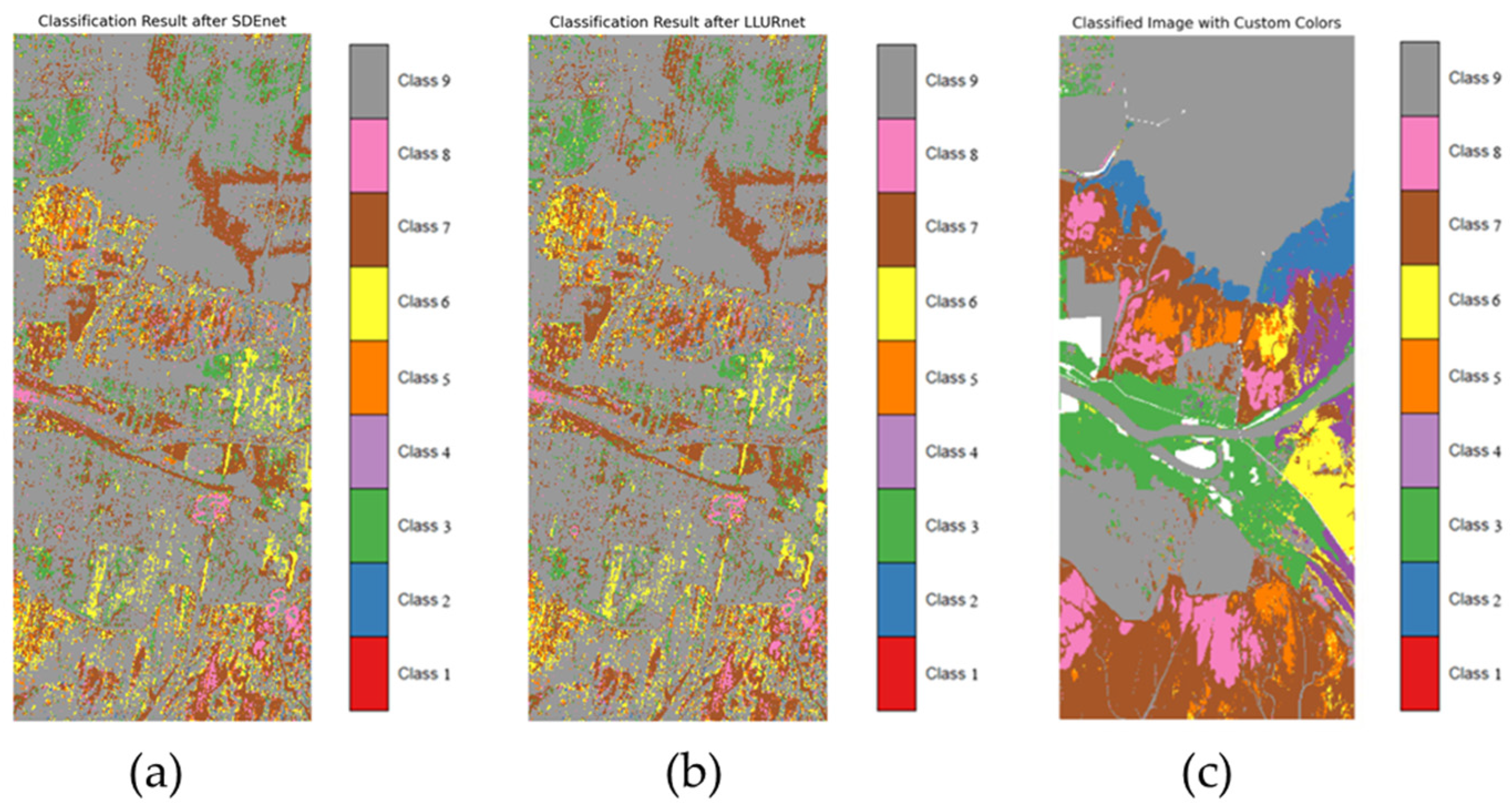
3.3. Semi Supervised Classification Test

Due to the poor generalization ability of unsupervised classification methods that solely rely on source domain images as training data in Section 3.1, semi-supervised classification is considered in the wetland cross-domain classification task, where a portion of the test data is reserved for training and the others are used for testing. Additionally, the adaptive spatial-spectral multiscale network (ASSMN) [42] is added as a representative of advanced deep learning algorithms for comparison.
In these two public datasets, there are a large number of training samples, which result in less dependence on the model and high classification accuracy, as shown in Table 9 and Table 10. However, for complex wetland landform distributions, the performance of various methods fluctuates greatly. As shown in Table 11 and Figure 7.
Utilize the entire GF-5 image data and 70% of the XG-003 image test data for training, while testing on the remaining 30% of the XG-003 image test data. Due to the data conflict between the training image and the test image, SVM and K-NN perform poorly on this task. Considering that the difference in spectral offset of water bodies with different satellite data may be small, while the difference in spectral offset of other vegetation is large, the classification accuracy is high only in the category with a large number of samples. The accuracy of the eighth type of water body in SVM and KNN methods is 0.5. The classification accuracy of other categories is extremely low, while the accuracy of the Class 2, Class 4, and Class 6 is slightly higher in ASSMN than in ours. This is attributed to ASSMN’s adoption of a band-grouping strategy and a multi-scale architecture for extracting multi-scale features, which excels in capturing long-sequence dependencies. However, there may be insufficient integration between different-scale information. By introducing double branches to improve the Transformer encoder, we use a convolutional multi-head self-attention unit, which can more effectively capture local and global spatial and spectral features, so that the model can not only focus on the important features of local areas but also understand the global pattern of the entire image. The dual-branch method, designed with two branches, enables more flexible integration of spatial and local-global spectral features. This design not only enhances the understanding of information across different scales but also facilitates more effective feature fusion, thereby improving classification accuracy. The classification accuracy of the other six categories and the overall accuracy are better than those of ASSMN, showing significant advantages in the classification of Spartina alterniflora, Tamarix chinensis Lour, and Phragmites australis. As seen in Figure 7, Class 3 Tamarix chinensis Lour predominantly coexists with Suaeda salsa or Phragmites australis, while Class 5, Phragmites australis on the Tidal Flats, exhibits a spectrum that is a mixture of Phragmites australis and tidal mud. In wetland application scenarios, our method simulates more spectral details of mixed images in the target domain within the 30% of additional target domain images learned. In the discriminator, the multi-scale spectral feature extraction module captures spectral features across various scales in the target domain. These processes collectively contribute to enhancing the accuracy of mixed vegetation classification tasks.
It is noteworthy that the spectra of Class 2 (Phragmites communis), Class 4 (Suaeda glauca Bunge), and Class 6 (Naked Tide Beach) are all influenced by water bodies. We need to further enhance our ability to eliminate the spectral impact of water bodies.

3.4. Ablation Test

To verify the effectiveness and robustness of the framework introduced in this paper for typical wetland feature classification, ablation experiments were conducted on the public datasets and the Yellow River Estuary Wetland dataset. Table 12, Table 13 and Table 14 show the test accuracy and overall accuracy on the single-branch CNN and the single-branch Transformer. The classification accuracy and overall accuracy of ours are generally higher than those of the single-branch models, which indicates that the original setting is more effective in wetland vegetation classification.
The Transformer model exhibits a certain degree of dependency on the quality and diversity of the training data. Meanwhile, CNN excels in its core capability of extracting local features. The dual-branch structure facilitates the extraction of features across different scales for vegetation, demonstrating robust performance globally and enhancing the model’s expressive power. The ablation experiment demonstrates that the dual-branch structure enhances the accuracy of wetland classification.

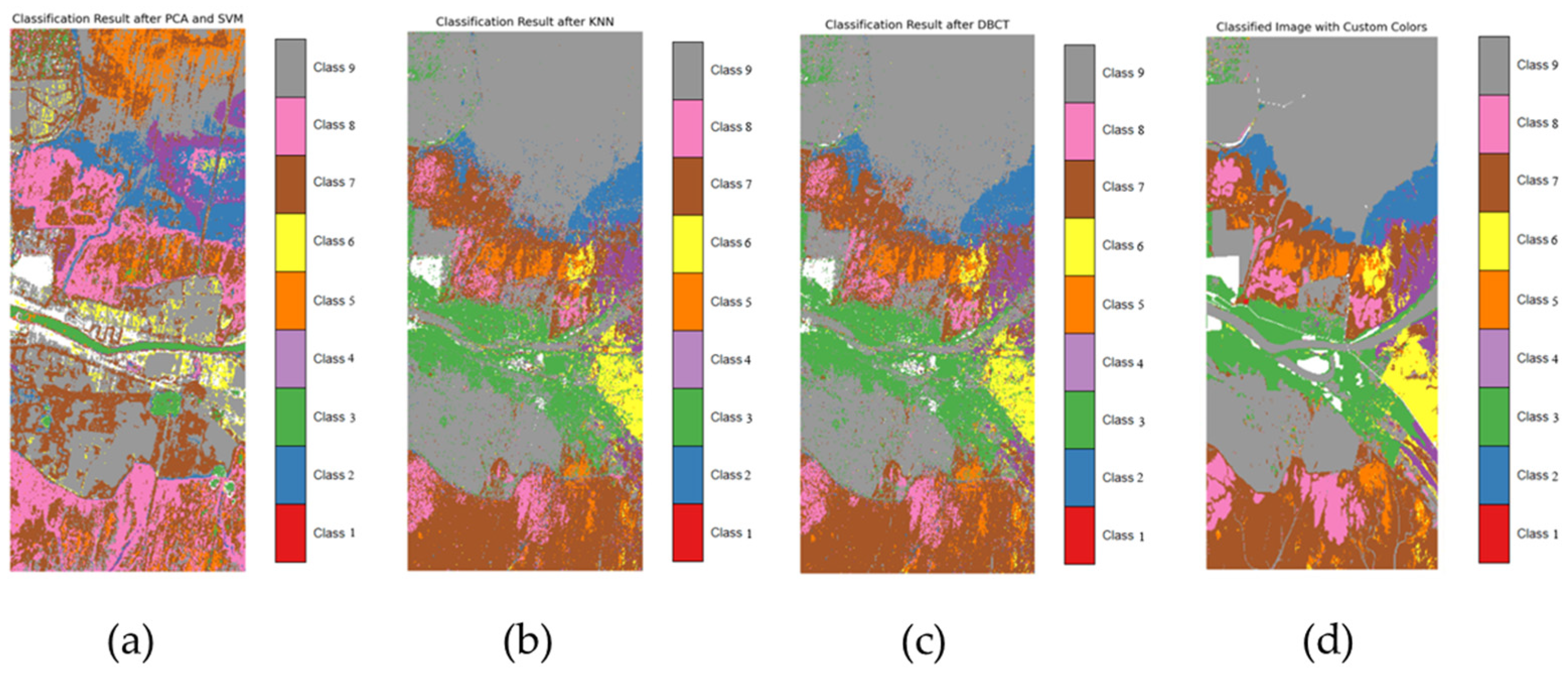
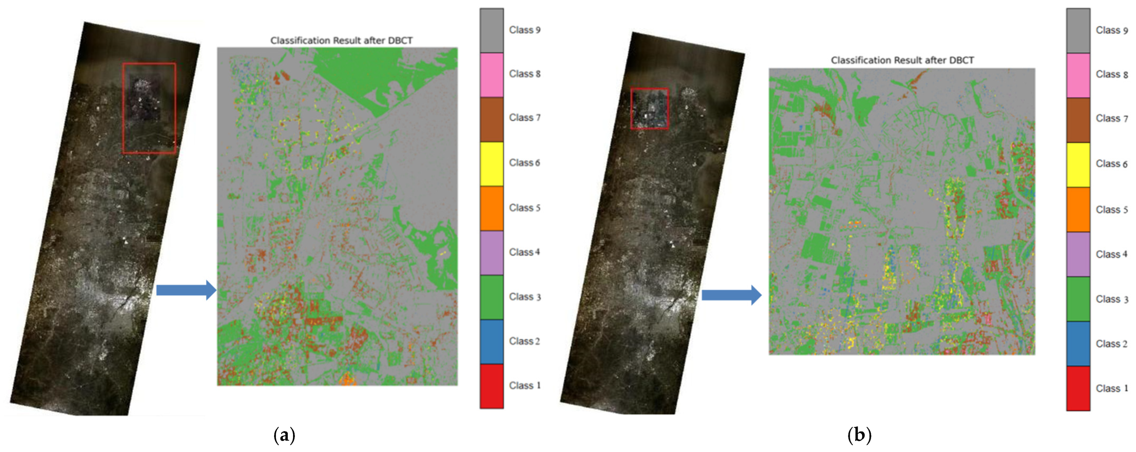
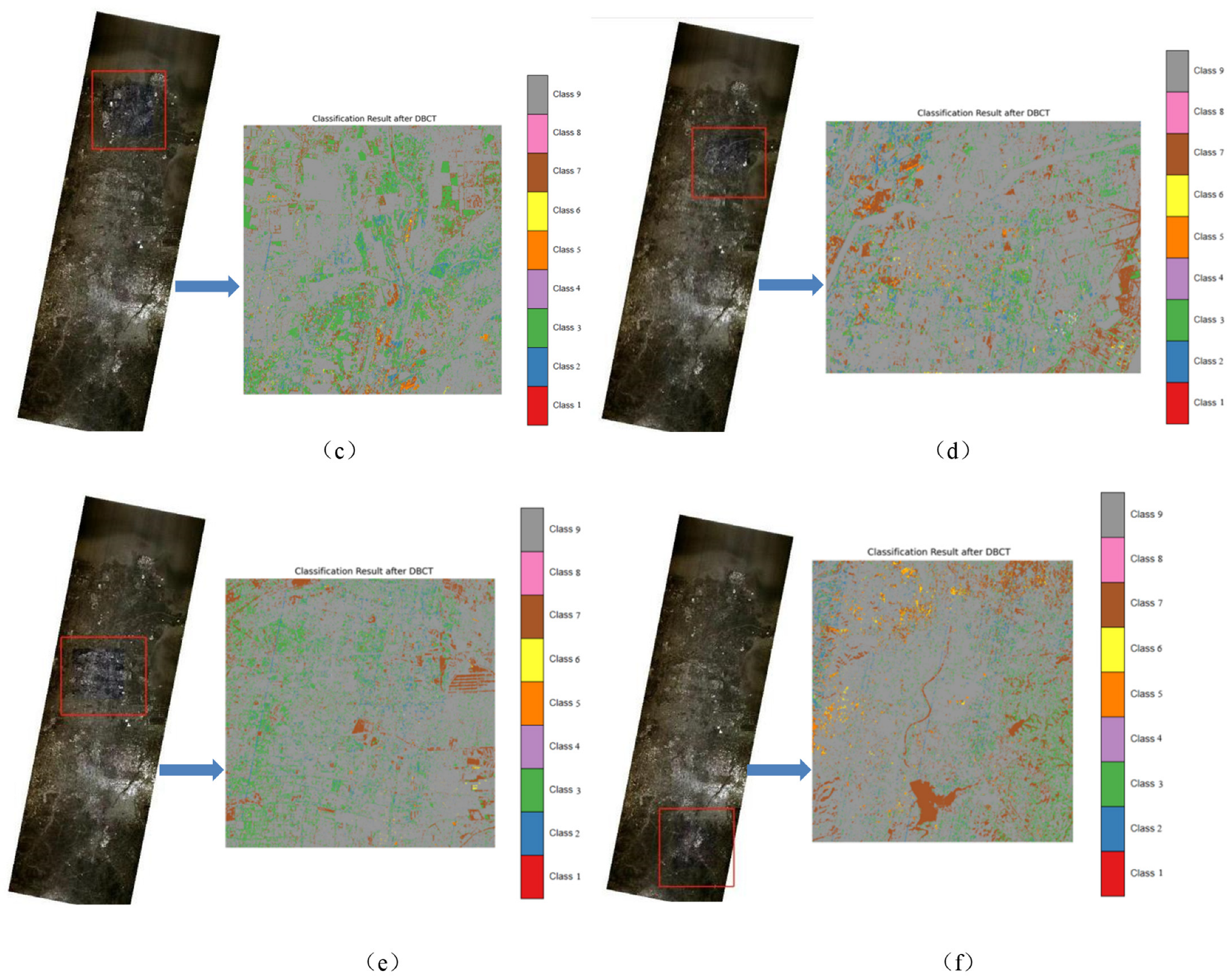
3.5. Vegetation Distribution in Yellow River Estuary Reserve

In the randomly cropped section of the XG-003 image, wetland land features are classified using the model in this paper. The visualization results are displayed in Figure 8. These images are taken in the Yellow River Estuary Nature Reserve, a region predominantly covered by water bodies. The tidal flat vegetation is sparse, with spartina alterniflora scattered sporadically on the seaward side. As shown in Figure 8a–c, the coverage rate of Tamarix chinensis Lour in the north of the region is high. In Figure 8e, the red box area is on both sides of the estuary, Suaeda salsa, Phragmites communis, and Tamarix chinensis Lour exhibit mixed growth. It illustrates the distribution of reeds and wetland beach patches in Figure 8f. In Figure 8a–f, the distribution of wetland species is generally consistent with the local elevation and the gradient of salinity [43]. As mentioned above, the semi-supervised model provides data support for wetland ecological monitoring.

4. Summary and Prospects

In response to the spectral deviations caused by atmospheric conditions and oceanic acoustic wave variations during the imaging process of different satellite hyperspectral sensors, as well as the varying spectral resolutions among sensors, a new task for cross-satellite classification of wetland vegetation hyperspectral images based on a linear unbiased random network is proposed. Considering that coastal wetland vegetation is mixed and influenced by water body spectra, to improve the generalization performance of the wetland vegetation cross-main classification model in unknown areas, we can better simulate the spectral drift of wetland vegetation data acquired by different satellites in the generator. Additionally, a multi-scale spectral feature extraction module is added to the discriminator, which facilitates the extraction of fine-scale information of small-patch wetland vegetation. In the self-made dataset, compared with classical methods and cutting-edge deep learning methods, the experimental results demonstrate better generalization capabilities. However, our research is still insufficient. We need to increase the number of experiments and improve experimental comparison methods. This is to verify the reliability of the model and its adaptability in wetland scenarios, such as TransUnet [44] and Swin HIS [45].
The method requires improvement in the future. Compared with other methods, the model presented in this manuscript is more complex and incurs higher computational costs. We can further optimize the generator and the loss function in subsequent work by generating manually mixed samples and incorporating on-site sampling annotations. We can also unmix the mixed spectrum of water and vegetation [46] or supplement the spectral data with light detection and ranging (LiDAR) data to eliminate the influence of the water spectrum of surrounding vegetation [47]. This will enhance the model’s performance for cross-scene classification and, consequently, improve the overall accuracy of vegetation classification.

Author Contributions

Conceptualization, Y.G.; Methodology, M.Y. and Y.G.; Software, M.Y.; Validation, Y.G.; Investigation, X.W. and Y.G.; Resources, J.Q.; Data curation, J.Q., X.W. and Y.G.; Writing—original draft, M.Y., J.Q. and X.W.; Writing—review & editing, M.Y.; Supervision, Y.G. All authors have read and agreed to the published version of the manuscript.

Funding

This research was funded by National Natural Science Foundation of China, grant number [62471160].

Data Availability Statement

The original contributions presented in this study are included in the article. Further inquiries can be directed to the corresponding author.

Conflicts of Interest

Author Jing Qin was employed by the company Xi’an Zhongke Xiguang Aerospace Science and Technology Co., Ltd. The remaining authors declare that the research was conducted in the absence of any commercial or financial relationships that could be construed as a potential conflict of interest.

References

  1. Sun, W.W.; Liu, W.W.; Wang, Y.M.; Zhao, R.; Huang, M.Z.; Wang, Y.; Yang, G.; Meng, X.C. Research progress and prospects of hyperspectral remote sensing for global wetland from 2010 to 2022. Natl. Remote Sens. Bull. 2023, 27, 1281–1299. [Google Scholar]
  2. Chen, P.S.; Tong, Q.X.; Guo, H.D. Research on Remote Sensing Information Mechanism; Science Press: Beijing, China, 1998; pp. 1–2. [Google Scholar]
  3. Zhao, Y.Q.; Yang, J.X. Hyperspectral image denoising via sparse representation and low-rank constraint. IEEE Trans. Geosci. Remote Sens. 2014, 53, 296–308. [Google Scholar] [CrossRef]
  4. Tuia, D.; Persello, C.; Bruzzone, L. Domain adaptation for the classification of remote sensing data: An overview of recent advances. IEEE Geosci. Remote Sens. Mag. 2016, 4, 41–57. [Google Scholar] [CrossRef]
  5. Torralba, A.; Efros, A.A. Unbiased look at dataset bias. In Proceedings of the IEEE Conference on Computer Vision and Pattern Recognition, Colorado Springs, CO, USA, 20–25 June 2011; pp. 1521–1528. [Google Scholar]
  6. Mateo-Garcia, G.; Laparra, V.; Lopez-Puigdollers, D.; Gomez-Chova, L. Cross-sensor adversarial domain adaptation of Landsat-8 and Proba-V images for cloud detection. IEEE J. Sel. Top. Appl. Earth Obs. Remote Sens. 2021, 14, 747–761. [Google Scholar] [CrossRef]
  7. Tuia, D.; Pasolli, E.; Emery, W.J. Using active learning to adapt remote sensing image classifiers. Remote Sens. Environ. 2011, 115, 2232–2242. [Google Scholar] [CrossRef]
  8. Chen, Y.S.; Lin, Z.H.; Zhao, X.; Wang, G.; Gu, Y.F. Deep learning-based classification of hyperspectral data. IEEE J. Sel. Top. Appl. Earth Obs. Remote Sens. 2014, 7, 2094–2107. [Google Scholar] [CrossRef]
  9. Li, Z.W.; Guo, F.M.; Ren, G.B.; Ma, Y.; Xin, Z.L.; Huang, W.H.; Sui, H.; Meng, Q. Hyperspectral remote sensing in the Yellow River Delta wetland. Mar. Sci. 2023, 47, 161–175. [Google Scholar]
  10. Goodfellow, I.J.; Pouget-Abadie, J.; Mirza, M.; Xu, B.; Warde-Farley, D.; Ozair, S.; Courville, A.; Bengio, Y. Generative adversarial nets. In Proceedings of the Advances in Neural Information Processing Systems (NIPS), Montreal, QC, Canada, 8–13 December 2014; pp. 2672–2680. [Google Scholar]
  11. Goodfellow, I.; Pouget-Abadie, J.; Mirza, M.; Xu, B.; Warde-Farley, D.; Ozair, S.; Courville, A.C.; Bengio, Y.Q. Generative adversarial networks. Commun. ACM 2020, 63, 139–144. [Google Scholar] [CrossRef]
  12. Zhong, Z.L.; Li, J.; Luo, Z.M.; Chapman, M. Spectral-spatial residual network for hyperspectral image classification: A 3-D deep learning framework. IEEE Trans. Geosci. Remote Sens. 2018, 56, 847–858. [Google Scholar] [CrossRef]
  13. Ganin, Y.; Ustinova, E.; Ajakan, H.; Germain, P.; Larochelle, H.; Laviolette, F.; Marchand, M.; Lempitsky, V. Domain-adversarial training of neural networks. J. Mach. Learn. Res. 2016, 17, 2096–3030. [Google Scholar]
  14. Long, M.S.; Cao, Z.J.; Wang, J.M.; Joedan, M.I. Conditional adversarial domain adaptation. In Proceedings of the 32nd International Conference on Neural Information Processing Systems, Montréal, QC, Canada, 3–8 December 2018. [Google Scholar]
  15. Tzeng, E.; Hoffman, J.; Saenko, K.; Darrell, T. Adversarial discriminative domain adaptation. In Proceedings of the IEEE Conference on Computer Vision and Pattern Recognition, Honolulu, HI, USA, 21–26 July 2017; pp. 7167–7176. [Google Scholar]
  16. Zhu, J.Y.; Park, T.; Isola, P.; Efros, A.A. Unpaired image-to-image translation using cycle-consistent adversarial networks. In Proceedings of the 2017 IEEE International Conference on Computer Vision, Venice, Italy, 22–29 October 2017; pp. 2223–2232. [Google Scholar]
  17. Zhang, Y.H.; Wu, J.Q.; Zhang, Q.; Hu, X.G. Multi-view feature learning for the over-penalty in adversarial domain adaptation. Data Intell. 2024, 1, 183–198. [Google Scholar] [CrossRef]
  18. Yi, Z.L.; Zhang, H.; Tan, P.; Gong, M.L. Dual GAN: Unsupervised dual learning for image-to-image translation. In Proceedings of the IEEE International Conference on Computer Vision (ICCV), Venice, Italy, 22–29 October 2017. [Google Scholar]
  19. Li, X.; Ma, J.; Wu, J.D.; Li, Z.R.; Tan, Z.Z. Transformer-based conditional generative transfer learning network for cross domain fault diagnosis under limited data. Sci. Rep. 2025, 15, 6836. [Google Scholar] [CrossRef]
  20. Li, W.C.; He, P.S.; Li, H.L.; Wang, H.X.; Zhang, R.M. Detection of GAN-Generated Images by Estimating Artifact Similarity Source. IEEE Signal Process. Lett. 2022, 29, 862–866. [Google Scholar] [CrossRef]
  21. Ma, X.P.; Zhang, X.K.; Wang, Z.G.; Pun, M.O. Unsupervised Domain Adaptation Augmented by Mutually Boosted Attention for Semantic. IEEE Trans. Geosci. Remote Sens. 2023, 61, 5400515. [Google Scholar]
  22. Xu, Y.H.; He, F.X.; Du, B.; Tao, D.C.; Zhang, L.P. Self-Ensembling GAN for Cross-Domain Semantic Segmentation. IEEE Trans. Multimed. 2023, 25, 7837–7850. [Google Scholar] [CrossRef]
  23. Zheng, X.T.; Xiao, X.L.; Chen, X.M.; Lu, W.X.; Liu, X.Y.; Lu, X.Q. Advancements in cross-domain remote sensing scene interpretation. J. Image Graph. 2024, 29, 1730–1746. [Google Scholar] [CrossRef]
  24. Yu, C.Y.; Liu, C.Y.; Song, M.P.; Chang, C.I. Unsupervised domain adaptation with content-wise alignment for hyperspectral imagery classification. IEEE Trans. Geosci. Remote Sens. 2021, 19, 5511705. [Google Scholar] [CrossRef]
  25. Ma, X.R.; Mou, X.R.; Wang, J.; Liu, X.K.; Geng, J.; Wang, H.Y. Cross-dataset hyperspectral image classification based on adversarial domain adaptation. IEEE Trans. Geosci. Remote Sens. 2020, 59, 4179–4190. [Google Scholar] [CrossRef]
  26. Wang, X.Z.; Liu, J.H.; Ni, Y.; Chi, W.J.; Fu, Y.Y. Two-stage domain alignment single-source domain generalization network for cross-scene hyperspectral images classification. IEEE Trans. Geosci. Remote Sens. 2024, 62, 5527314. [Google Scholar] [CrossRef]
  27. Bejiga, M.B.; Melgani, F. An adversarial approach to cross-sensor hyperspectral data classification. In Proceedings of the IGARSS 2018 IEEE International Geoscience and Remote Sensing Symposium, Valencia, Spain, 22–27 July 2018; pp. 3575–3578. [Google Scholar]
  28. Kalita, I.; Kumar, R.N.S.; Roy, M. Deep learning-based cross-sensor domain adaptation under active learning for land cover classification. IEEE Trans. Geosci. Remote Sens. 2021, 19, 6005005. [Google Scholar] [CrossRef]
  29. Mahmoudi, A.; Ahmadyfard, A. A GAN-based method for cross-scene classification of hyperspectral scenes captured by different sensors. Multimed. Tools Appl. 2024. [Google Scholar] [CrossRef]
  30. Wang, J.Y.; Wang, Y.M.; Li, C.L. Noise model of hyperspectral imaging system and influence on radiation sensitivity. J. Remote Sens. 2010, 14, 607–620. [Google Scholar]
  31. Sun, H.Z. Research on Hyperspectral Remote Sensing Image Denoising Method and Its Application in Target Detection. Ph.D. Thesis, Harbin Institute of Technology, Harbin, Chian, 2022. [Google Scholar]
  32. Zhou, Q.Z.; Guo, Q.; Wang, H.R.; Li, A. Two discriminators deep residual GAN hyperspectral image pan-sharpening. J. Image Graph. 2024, 29, 2046–2062. [Google Scholar] [CrossRef]
  33. Hu, Y.B.; Ren, G.B.; Ma, Y.; Yang, J.F.; Wang, J.B.; An, J.B.; Liang, J.; Ma, Y.Q.; Song, X.K. Coastal wetland hyperspectral classification under the collaborative of subspace partition and infinite probabilistic latent graph ranking. Sci. China (Technol. Sci.) 2022, 65, 759–777. [Google Scholar] [CrossRef]
  34. Cover description. Hyperspectral pseudo color image of lakes on the Gongzhucuo Plateau in Tibet obtained by Xiamen Science and Technology No.1 satellite. Natl. Remote Sens. Bull. 2024, 28, 321. [Google Scholar]
  35. Xu, R.; Dong, X.M.; Li, W.; Peng, J.T.; Sun, W.W.; Xu, Y. DBCT Net: Double branch convolution-transformer network for hyperspectral image classification. IEEE Trans. Geosci. Remote Sens. 2024, 62, 5509915. [Google Scholar]
  36. Chen, Y.L.; Teng, W.T.; Li, Z.; Zhu, Q.Q.; Guan, Q.F. Cross-domain scene classification based on a spatial generalized neural architecture search for high spatial resolution remote sensing images. Remote Sens. 2021, 13, 3460. [Google Scholar] [CrossRef]
  37. Zhu, S.; Pan, X.; Li, X. Effect of Spartina spp. invasion on saltmarsh community of the Yellow River Delta. Shandong Agric. Sci. 2012, 44, 73–75, 83. [Google Scholar]
  38. Zhang, Y.X.; Li, W.; Sun, W.D.; Tao, R. Single-source domain expansion network for cross-scene hyperspectral image classification. IEEE Trans. Image Process. 2023, 32, 1498–1512. [Google Scholar] [CrossRef]
  39. Zhao, H.Q.; Zhang, J.W.; Lin, L.L.; Wang, J.K.; Gao, S.; Zhang, Z.W. Locally linear unbiased randomization network for cross-scene hyperspectral image classification. IEEE Trans. Geosci. Remote Sens. 2023, 61, 5526512. [Google Scholar] [CrossRef]
  40. Cortes, C.; Vapnik, V. Support-vector networks. Mach. Learn. 1995, 20, 273–297. [Google Scholar] [CrossRef]
  41. Cunningham, P.; Delany, S.J. k-Nearest neighbour classifiers—A tutorial. ACM Comput. Surv. (CSUR) 2021, 54, 128. [Google Scholar] [CrossRef]
  42. Wang, D.; Du, B.; Zhang, L.; Xu, Y. Adaptive spectral–spatial multiscale contextual feature extraction for hyperspectral image classification. IEEE Trans. Geosci. Remote Sens. 2021, 59, 2461–2477. [Google Scholar] [CrossRef]
  43. An, L.S.; Zhou, B.H.; Zhao, Q.S.; Wang, L. Spatial distribution of vegetation and environmental interpretation in the Yellow River Delta. Acta Ecol. Sin. 2017, 37, 6809–6817. [Google Scholar]
  44. Chen, J.N.; Lu, Y.Y.; Yu, Q.H.; Luo, X.D.; Adeli, E.; Wang, Y.; Lu, L.; Alan, L.Y.; Zhou, Y.Y. TransUNet: Transformers Make Strong Encoders for Medical Image Segmentation. arXiv 2021, arXiv:2102.04306. [Google Scholar] [CrossRef]
  45. Cao, H.; Wang, Y.Y.; Chen, J.; Jiang, D.S.; Zhang, X.P.; Tian, Q.; Wang, M.N. Swin-Unet: Unet-like Pure Transformer for Medical Image Segmentation. In Proceedings of the Computer Vision—ECCV 2022 Workshops, Tel Aviv, Israel, 23–27 October 2022; pp. 205–218. [Google Scholar]
  46. Kamal, M.; Phinn, S. Hyperspectral Data for Mangrove Species Mapping: A Comparison of Pixel-Based and Object-Based Approach. Remote Sens. 2011, 3, 2222–2242. [Google Scholar] [CrossRef]
  47. Guo, F.M.; Li, Z.W.; Ren, J.B.; Wang, L.Q.; Zhang, J.; Wang, J.B.; Hu, Y.B.; Yang, M. Instance-Wise Domain Generalization for Cross-Scene Wetland Classiffcation with Hyperspectral and LiDAR Data. IEEE Trans. Geosci. Remote Sens. 2024, 63, 5501212. [Google Scholar]
Figure 1. Structure diagram of cross-satellite hyperspectral image classification method based on the linear randomized network. There are two modules, i.e., Generator (G) and Discriminator (D). G generates simulated images by reconstructing data from the learned domain-discriminative representation. D consists of three basic steps: Step 1: a 1 × 1 × 7 3D convolution layer is employed for dimensionality reduction. Step 2: Multi-scale spectral feature extraction module. This module extracts the features of the original training image, the simulated image output by the generator, and the mixed image obtained by the linear combination of the two. Step 3: 3D CNN and Transformer encoder module, this module carries out joint extraction of spatial and spectral features.
Jmse 13 00801 g001
Figure 2. Self-made dataset of GF-5 hyperspectral images of the Yellow River Estuary Wetland (Pseudo-color generation from random three bands). (a) Original truth map and sample count; (b) Trimmed image and sample count.
Jmse 13 00801 g002
Figure 3. Self-made dataset of XG-003 hyperspectral images of the Yellow River Estuary Wetland (Pseudo-color generation from three random bands).
Jmse 13 00801 g003
Figure 4. Classification results of different methods on cross-domain hyperspectral images. (a) Classification results of SDE net. (b) Classification results of LLU net. (c) True value.
Jmse 13 00801 g004
Figure 5. Visual classification results of different methods on GF-5 images. (a) Classification results of SVM. (b) Classification results of K-NN. (c) Classification results of ours. (d) True value.
Jmse 13 00801 g005
Figure 6. Visual classification results of different methods on XG-003 images. (a) Classification results of SVM. (b) Classification results of K-NN. (c) Classification results of ours. (d) True value.
Jmse 13 00801 g006
Figure 7. Visualization results of XG-003 on semi-supervised hyperspectral image classification using different methods. (a) Classification results of SVM. (b) Classification results of K-NN. (c) Classification results of ours. (d) Classification results of ASSMN. (e)True value.
Jmse 13 00801 g007
Figure 8. Visualization results of the classification of the XG-003 image by a semi-supervised method. (af) Visualization of the distribution of random wetland features. On the left is the original XG-003 hyperspectral image, with the red box indicating a randomly cropped area. On the right is the visualization of wetland surface feature classification results obtained using a semi-supervised method.
Jmse 13 00801 g008aJmse 13 00801 g008b
Table 1. Number of source and target samples for the Pavia dataset.
ClassNumber of Samples
No.NamePavia U
(Source)
Pavia C
(Target)
1Tree30647598
2Asphalt66319248
3Bricks36822685
4Bitumen13307287
5Shadows9472863
6Meadows18,6493090
7Bare soil50296584
Total39,33239,355
Table 2. Number of source and target samples for the Shanghai-Hangzhou dataset.
ClassNumber of Samples
No.NameShanghai
(Source)
Hangzhou
(Target)
1Water18,043123,123
2Land/Building77,450161,689
3Plant40,20783,188
Total135,700368,000
Table 3. Comparison of technical parameters between GF-5 and XG-003 hyperspectral imaging.
SatelliteTrack Height (km)Width (km)Spatial Resolution (m)Number of Spectral Channels (Number)Spectral Range
(nm)
Spectral Resolution
(nm)
Time
GF-57056030330400–2500VNIR: 5 nm
SWIR: 10 nm
1 November 2018
XG-0035308040150430–8503 nm28 September 2024
Table 4. Number of source and target samples for the GF-5 and XG-003 dataset.
ClassNumber of Samples
No.NameGF-5
(Source)
XG-003
(Target)
1Spartina alterniflora63175452
2Phragmites australis15,51714,814
3Tamarix chinensis Lour14,2434363
4Suaeda glauca Bunge11,5244534
5Phragmites australis on the Tidal Flats99345202
6Naked Tide Beach22,38930,424
7Salt Marsh52087392
8Water Body15,87559,842
9Others22952271
Total103,302134,294
Table 5. Legend representation of coastal wetland features.
Ground ObjectsSpartina alternifloraPhragmites australisTamarix chinensis LourSuaeda glauca BungePhragmites australis on the Tidal FlatsNaked Tide BeachSalt MarshWater BodyOthers
Categoryclass1class 2class 3class 4class 5class 6class 7class 8class 9
Legend
Table 6. Accuracy of various cross-domain algorithms on test images.
MethodOA (%)AA (%)
SDE net [38]0.430.11
LLU net [39]0.450.16
Table 7. Classification accuracy of different algorithms on training data and test images (GF-5).
Method123456789OA (%)AA (%)
SVM [40]0.710.540.530.510.40.540.640.660.460.560.56
K-NN [41]0.870.740.760.740.660.760.840.930.810.780.79
Ours0.910.820.850.750.710.780.880.840.720.810.81
Table 8. Classification accuracy of different algorithms on training data and test images (XG-003).
Method123456789OA (%)AA (%)
SVM [40]0.210.380.030.090.140.480.280.610.370.430.29
K-NN [41]0.760.790.620.540.660.830.650.890.450.810.76
Ours0.940.880.830.760.820.810.880.910.840.870.85
Table 9. Comparative experiment on the Pavia dataset.
Method1234567OA (%)AA (%)
SVM [40]0.920.800.840.850.900.780.790.940.84
K-NN [41]0.800.780.780.900.810.820.830.960.84
ASSMN [42]0.991.000.990.991.000.991.000.990.99
Ours0.991.000.990.991.000.991.000.990.99
Table 10. Comparative experiment on the Shanghai-Hangzhou dataset.
Method123OA (%)AA (%)
SVM [40]0.991.001.001.000.99
K-NN [41]0.990.990.980.990.99
ASSMN [42]1.001.001.001.001.00
Ours1.001.001.001.001.00
Table 11. Comparative experiment on the GF-5-XG-003 dataset.
Method123456789OA (%)AA (%)
SVM [42]0.020.050.040.010.010.070.060.50.040.180.09
K-NN [43]0.030.110.040.10.050.260.040.50.000.380.13
ASSMN [44]0.890.840.840.860.630.890.850.810.680.810.81
Ours0.910.820.850.750.710.780.880.840.720.870.86
Table 12. Ablation experiment on the Pavia dataset.
Experimental SetupOA (%)AA (%)
Original settings 0.990.99
Single-branch CNN 0.970.98
Single-branch Transformer 0.990.98
Table 13. Ablation experiment on the Shanghai-Hangzhou dataset.
Experimental SetupOA (%)AA (%)
Original settings 1.001.00
Single-branch CNN 1.000.99
Single-branch Transformer 0.990.99
Table 14. Ablation experiment on the GF-5-XG-003 dataset.
Experimental SetupOA (%)AA (%)
Original settings 0.870.86
Single-branch CNN 0.780.70
Single-branch Transformer 0.790.69
Disclaimer/Publisher’s Note: The statements, opinions and data contained in all publications are solely those of the individual author(s) and contributor(s) and not of MDPI and/or the editor(s). MDPI and/or the editor(s) disclaim responsibility for any injury to people or property resulting from any ideas, methods, instructions or products referred to in the content.

