Improved Snake Optimization and Particle Swarm Fusion Algorithm Based on AUV Global Path Planning

Abstract

An improved snake optimization algorithm (ISO) is proposed to obtain an effective and reliable three-dimensional path for an autonomous underwater vehicle (AUV) to navigate seabed barrier environments and ocean currents. First, a three-dimensional seafloor environment model, seafloor obstacles, and a model of a Lamb vortex current are constructed. Second, the designed mathematical framework for three-dimensional path planning comprehensively considers a variety of constraints such as sailing distance, path threat, sailing altitude, and optimized ocean current energy consumption. Finally, ISO diversifies the snake population’s distribution space by implementing a good point set initialization approach, a Cauchy variation strategy to enhance the convergence accuracy, and a fusion particle swarm algorithm strategy to improve the convergence speed. To evaluate ISO’s optimization performance, by minimizing the fitness value, the optimization outcomes are contrasted with those of five different algorithms. The experimental results show that the ISO algorithm can generate safe, low-energy, and path-optimal AUV navigation planning, which presents a novel effective approach for AUV path planning.

1. Introduction

The usage and development of maritime resources cannot be separated from the support of AUVs, which are crucial to the execution of marine science missions’ autonomous adaptive sampling [1], seafloor surveys, and reconnaissance [2]. In order to adapt to the needs of future ocean development, there are higher requirements for the autonomy of AUVs. The key technologies for accomplishing AUV sailing [3], path planning, and obstacle avoidance will dictate the future of AUV applications.

Most of the existing underwater path-planning studies focus on two-dimensional paths [4], without considering issues such as sailing altitude and energy saving by using ocean currents. Therefore, it has become a current research hotspot to design a reasonable fitness function so that the AUV can plan a path using ocean currents for energy saving, obstacle avoidance, and path optimization via three-dimensional path planning.

Currently, many experts have proposed different methods to be applied in AUV path planning, like graph search, potential field approach, bionic algorithm, and reinforcement learning. Graph-search-based path planning, such as that proposed by Jiu et al. [5], is designed to obtain the source location based on a partially observable Markov decision and use the A* search algorithm to find the shortest path to the chemical source, but there is a search space that is too high. Path planning based on potential field methods such as a closed-loop rapid exploration random tree (CL-RRT) algorithm was presented by Taheri et al. [6] to solve the motion constraints caused by obstacles and the characteristics of AUVs but failed to take into account the use of ocean currents to conserve energy. Based on bionic algorithms, Yan et al. [7] suggested an improved genetic algorithm that solves the premature problem of traditional genetic algorithms, but improper parameter settings in these algorithms can result in slower planning. Mahmoud et al. [8] optimized the control points generated by B-splines with a differential evolutionary algorithm and succeeded in enabling an AUV to avoid obstacles. Lim et al. [9] proposed an algorithm that combines a selective differential evolutionary algorithm and a particle swarm optimization algorithm, which were fused to successfully complete offline path planning for AUVs. Che et al. [10] proposed an ant colony algorithm combined with particle swarm optimization to make the algorithm search for optimal paths faster. Machine-learning-based path planning, such as that proposed by Cao et al. [11], is a hierarchical reinforcement learning method based on potential fields to improve the collaboration efficiency of AUVs. Deep reinforcement learning: 2D sonar images were one of the state inputs utilized by Havenstrøm et al. [12] in their study, and the system’s output was passed through a low-pass filter before being used by the control fins to accomplish obstacle avoidance and course-tracking functions. Although the reinforcement learning planned a better path for the AUV, there are still problems such as low sample efficiency. Liang et al. [13] proposed AUV path planning to find a solution to reach a specified destination in the shortest possible time from a known initial position.

In order for the algorithm to achieve security, energy saving, and a global optimal solution, this paper first constructs a three-dimensional underwater environment model and an adaptive function model by comprehensively considering the effectiveness of the path, security, and the utilization of the ocean current rate. At the same time, for the original snake algorithm population initialization solution, the initial spatial distribution is uneven, making it easy to fall into the local optimum, and finding the optimal precision is not high. In this paper, a multi-strategy improvement of the snake algorithm (ISO) is proposed: the good point set mapping strategy is introduced for the initialization of the population to ensure an even distribution; the PSO algorithm is incorporated to improve the convergence speed; and the Cauchy variation strategy improves the algorithm’s precision of convergence and its capacity to leap out of the local optimum. To verify the superiority of ISO, simulation experiments are conducted to compare it with SO, JSO, PSO, ICFPSO, and WOA, and the results show that ISO can find the global optimal solution with higher accuracy in fewer iterations.

The structure of the paper is as follows. The 3D seafloor and ocean current environment models are presented in Section 2. The objective function for AUV path planning is presented in Section 3. Section 4 describes how the SO algorithm can be improved. Section 5 describes the simulations and analyses. And lastly, the study’s work is summarized in Section 6.

2. Problem Formulation

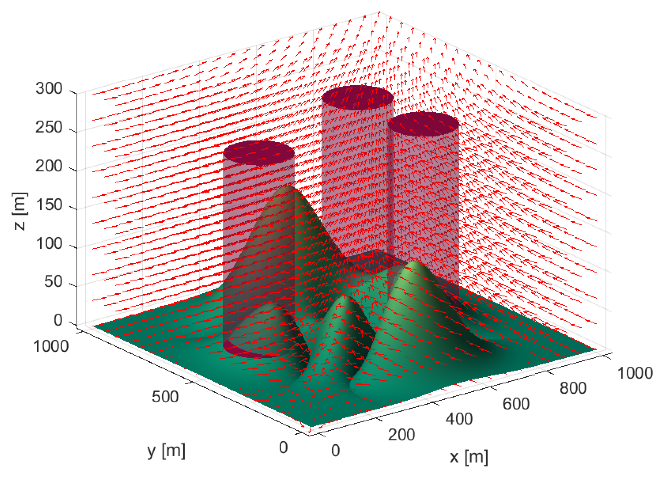
2.1. Modeling of the Underwater Environment in Three Dimensions

The topography of the seabed exhibits notably unstructured features, with its geomorphology defined by ridges, seamounts, and various other geological formations. When an AUV navigates in close proximity to the ocean floor, it must adapt its route according to the diverse seabed terrain it encounters. Consequently, the importance of establishing a precise environmental model cannot be overstated for planning an optimal path. In this paper, we use the literature [14], (Equation (1)), to generate a 1000 × 1000 × 300 model of the underwater environment; the height is adjusted to 20 times the absolute value, and the modeling function is detailed below:

$$Z=3{\left(1-x\right)}^2{e}^{-x^2-{\left(y+1\right)}^2}-10\left({\displaystyle \frac{x}{5}}-x^3-y^5\right)e^{-x^2-y^2}-{\displaystyle \frac{1}{3}}{e}^{-{\left(x+1\right)}^2-y^2}$$

(1)

where $x,y$ values range from −3 to 3.

2.2. Ocean Current Model

Acquiring data on ocean currents is of importance for AUV path planning, given that these flows can greatly influence the vehicles’ trajectories and energy expenditure. Commonly used methods to obtain current information include satellite observation, numerical prediction, and radar measurement. Each of these approaches has unique benefits and drawbacks: satellite observation has a wide coverage but poor real-time performance; high-frequency ground-wave radar measurements have high accuracy but are limited by equipment. In this study, an ocean current model with several eddies overlaid is established using the numerical method suggested in the literature [15], which can better simulate the characteristics of ocean currents in a complex marine environment and provide a reliable current information basis for AUV path planning. The specific formulas are as follows:

$$\left\{\begin{array}{c}{V}_x\left(\overrightarrow{r}\right)=-\Gamma {\displaystyle \frac{y-y_0}{2\pi ‖\overrightarrow{r}-\overrightarrow{r_0}‖}}\left(1-e^{-\left({\displaystyle \frac{{‖\left(\overrightarrow{r}-\overrightarrow{r_0}\right)‖}^2}{{\sigma }^2}}\right)}\right)\\ V_y\left(\overrightarrow{r}\right)=\Gamma {\displaystyle \frac{x-x_0}{2\pi ‖\overrightarrow{r}-\overrightarrow{r_0}‖\left(\overrightarrow{r}-\overrightarrow{r_0}\right)}}\left(1-e^{-\left({\displaystyle \frac{{‖\left(\overrightarrow{r}-\overrightarrow{r_0}\right)‖}^2}{{\sigma }^2}}\right)}\right)\\ {\omega }_z\left(\overrightarrow{r}\right)={\displaystyle \frac{\Gamma }{\pi \sigma }}{e}^{-\left({\displaystyle \frac{{‖\overrightarrow{r}-\overrightarrow{r_0}‖}^2}{{\sigma }^2}}\right)}\end{array}\right.$$

(2)

where $V_x\left(\stackrel{⃑}{r}\right)$, $V_y\left(\stackrel{⃑}{r}\right)$, $\mathrm{a}\mathrm{n}\mathrm{d} {\omega }_z\left(\stackrel{⃑}{r}\right)$ are the vortex current velocity components in the horizontal, longitudinal, and vertical directions. $\Gamma , \sigma ,$ and ${\stackrel{⃑}{r}}_0$ are the coordinates of the vortex current intensity, vortex current radius, and eddy current center position.

In Figure 1, the ocean current’s direction is indicated by the red arrow. The sailing speed of the AUV is a vector synthesis of the hydrostatic and ocean current speeds, and its speed is affected by the ocean currents, with the heading determined from $x_i$ to ${ x}_{i+1}$. and it converts the energy consumption approach to the key optimization parameters in the cost function $j_4$ When the heading is in the same direction as the current, the cost of sailing time $j_4$ decreases, while when the opposite is obstructed, the cost of sailing time $j_4$ increases. The red cylinders and green seamounts in the model represent obstacles.

3. Objective Function

By defining an objective function, this work converts the path-planning problem into a multi-objective optimization problem, which takes into account the four factors of the AUV’s sailing distance, path threat, sailing altitude, and the cost of current constraints to establish a fitness function to determine whether the generated path is the optimal solution or not. The design of the fitness function is as follows:

$$minJ=J_1+J_2+J_3+J_4$$

(3)

where, $J_1$ represents the cost of navigational distance, ${ J}_2$ represents the cost of path threat, $J_3$ represents the cost of navigational altitude, and $J_4$ represents the cost of current constraint.

3.1. Distance Cost

The sailing distance function is used to compute the sailing distance of the AUV from the initial coordinates to the terminal coordinates with the following function:

$$J_1=\sum _{i=1}^{n-1}\sqrt{{\left(x_{i+1}-x_i\right)}^2+{\left(y_{i+1}-y_i\right)}^2+{\left(z_{i+1}-z_i\right)}^2}$$

(4)

where total distance travelled consists of $n$ waypoints. $\left(x_i,y_i,z_i\right)$ and $\left(x_{i+1},y_{i+1},z_{i+1}\right)$ denote the 3D coordinates of the $i$ navigational point and the $i+1$ navigational point.

3.2. Path Threat Constraint Cost

As the AUV navigates a path closer to the obstacle, the risk to the AUV increases. In the literature [16], the percentage of AUVs entering the hazardous area is used to determine whether the cost value increases or not, and this constraint lacks mathematical quantification, making it difficult for the optimization algorithm to accurately avoid obstacles. In contrast, in this paper, a segmentation function is used to strictly quantify the threat cost so that the AUV can effectively avoid undersea obstacles. The path threat object constraint can be expressed as follows:

$$J_2=\sum _{i=1}^{threa{t}_{num}}\sum _{j=1}^{n-1}{threa{t}_{cost}}_{i,j}$$

(5)

where ${threat\_cost}_{i,j}$ represents the threat cost between the $i$ segment of the path and the $j$ obstacle, given as

$$\begin{array}{c}threa{t}_{cost}=\\ \left\{\begin{array}{c}{J}_{\mathrm{\infty }}\\ \left(r_t+r_s+r_d\right)-d_{i,j}\\ 0\end{array}\right. \begin{array}{c}{d}_{i,j}<\left(r_t+r_s\right)\\ \left(r_t+r_d\right)<d_{i,j}\le \left(r_t+r_s+r_d\right)\\ d_{i,j}>\left(r_t+r_s+r_d\right)\end{array}\end{array}$$

(6)

where $d_{i,j}$ represents the distance of the path from the threat, $r_{t }$ represents the radius of the threat, $r_s$ represents AUV size, and $r_d$ represents hazard distance.

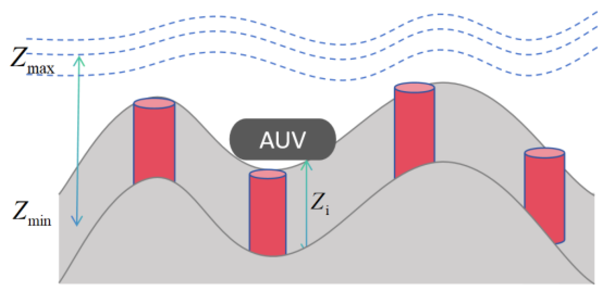
3.3. Altitude Constraint Cost

In the path planning of an AUV, existing studies, such as [17], focus only on obstacle avoidance and path optimization in the two-dimensional plane, and their models do not take into account the problem of altitude (z-direction) on navigation safety and energy consumption. To address this problem, this paper adopts a trip altitude function to ensure that the trip altitude of the AUV is kept within a reasonable range to avoid a too high or too low trip altitude. Too high a navigational altitude may expose the AUV to hazardous currents, while too low a navigational altitude may increase the risk of collision with the seabed or an obstacle. The constraint formula for the height of travel is shown below:

$$J_3=\sum _{i=1}^n{j}_{3_i}$$

(7)

where $j_{3_i}$ represents the height cost of the $i$ node, which is used to measure the degree of deviation between the height of the AUV at each path node and the reference height. The $j_{3_i}$ function is as follows:

$$j_{3_i}=\left\{\begin{array}{c}{j}_{\infty }\\ \left|z_i-\left.{\displaystyle \frac{z_{\mathrm{m}\mathrm{a}\mathrm{x}}+z_{\mathrm{m}\mathrm{i}\mathrm{n}}}{2}}\right|\right.\end{array}\right.\begin{array}{c}{z}_i\le 0\\ z_i>0\end{array}$$

(8)

Figure 2 simulates the case of the navigational altitude of the AUV, which is considered to be invalid when the altitude of a node $z_i\le 0$ in the three-dimensional space. This is because it is impossible for an AUV to navigate with zero or negative underwater altitude. At this point, the node cost $j_{3_i}$ is defined as an infinite $j_{\infty }$. For the effective altitude ($z_i>0$), $j_{3_i}$ represents the absolute difference between the node altitude and the reference altitude $\left|z_i-\left.{\displaystyle \frac{z_{\mathrm{m}\mathrm{a}\mathrm{x}}+z_{\mathrm{m}\mathrm{i}\mathrm{n}}}{2}}\right|\right.$. This reference altitude is the intermediate value between the maximum permissible altitude $z_{\mathrm{m}\mathrm{a}\mathrm{x}}$ and the minimum permissible navigational altitude $z_{\mathrm{m}\mathrm{i}\mathrm{n}}$ and indicates a relatively safe and appropriate altitude for AUV navigation.

3.4. Current Constraint Cost

Established studies (e.g., literature [18]) mostly adopt a two-dimensional ocean current modeling paradigm, which reduces the ocean flow to the horizontal velocity component and ignores the vertical velocity component problem. The three-dimensional ocean current model adopted in this paper can solve this problem.

It is assumed that the hydrostatic speed is constant during AUV navigation; this assumption simplifies the dynamic control model of the propulsion system and allows the path-planning algorithm to focus on optimizing the synergy between the currents and heading, The current velocity $V_o$, and the direction of navigation is set to $\left(x_i,y_i,z_i\right)$ to $\left(x_{i+1},y_{i+1},z_{i+1}\right)$. The navigation velocity of the AUV $V_{ai}$ is the vector of the hydrostatic velocity $V$ and the current velocity $V_{oi}$ at the point ${ x}_i$.

$$\left\{\begin{array}{c}{V}_{ai}sin{\theta }_{ai}=V_{s}sin{\theta }_{si}+V_{oi}sin{\theta }_{oi}\\ V_{ai}cos{\theta }_{ai}=V_{s}cos{\theta }_{si}+V_{oi}cos{\theta }_{oi}\end{array}\right.$$

(9)

According to the triangular relationship, we can obtain

$${V_{ai}=V_{oi}\mathit{cos}\left({\theta }_{ai}-{\theta }_{oi}\right)+V_s\left[1-{\left({\displaystyle \frac{V_{oi}}{V_s}}\right)}^{2}sin\left({\theta }_{ai}-{\theta }_{oi}\right)\right]}^{{\displaystyle \frac{1}{2}}}$$

(10)

where ${\theta }_{ai}$, ${\theta }_{si}$, and ${\theta }_{oi}$ denote the angle between the total velocity, hydrostatic velocity, and current velocity, and for horizontal cutting direction $i$, counterclockwise is positive.

In the literature [19], it is suggested that the current constraints on AUVs can be converted into a navigation time cost. Consequently, each path segment’s navigation time is

$$t_{i,i+1}={\displaystyle \frac{l_{i,i+1}}{\left|V_{ai}\right|}}$$

(11)

where $l_{i,i+1}=\sqrt{{\left(x_{i+1}-x_i\right)}^2+{\left(y_{i+1}-y_i\right)}^2+{\left(z_{i+1}-z_i\right)}^2}$.

Then, the current constraint function is as follows:

$$j_4=\sum _{i=1}^{n-1}{t}_{i,i+1}$$

(12)

4. AUV Path Planning Based on ISO Algorithm

4.1. Snake Optimizer

Snake optimizer (SO) is an algorithm based on the optimal simulation of snakes proposed by Fatma A. Hashim and Abdelazim G. Hussie [20] in 2022. The snake population is split up by the algorithm into 50% males and 50% females, which then simulates temperature, amount of food, snakes searching for food, moving toward food, fighting, mating, and egg-laying sociosexual behavior. SO divides the iteration into “global exploration” and “local exploitation”, which effectively balances the range of the path. The mathematical expressions for the different models are given below.

The algorithm sets the temperature threshold to 0.25 and the food quantity threshold to 0.6.

$$\left\{\begin{array}{c}Temp=\exp \left(-{\displaystyle \frac{t}{T}}\right)\\ Q=c_1\left(-{\displaystyle \frac{t}{T}}\right)\end{array}\right.$$

(13)

where $t$ denotes the current iteration number, $T$ denotes the maximum iteration number, $c_1=0.5$, $Temp$ denotes the temperature, and $Q$ denotes the food quantity.

When $Q<0.25$, the snake algorithm enters the food-seeking mode.

$$\left\{\begin{array}{c}{A}_m=\mathit{exp}\left({\displaystyle \frac{-f_{rand,m}}{f_{i,m}}}\right)\\ X_{i,m}\left(t+1\right)=\\ X_{rand,m}\left(t\right)\pm c_2\times A_m\times \left(\left(X_{max}-X_{min}\right)\times rand+X_{min}\right)\end{array}\right.$$

(14)

$$\left\{\begin{array}{c}{A}_f=\mathit{exp}\left({\displaystyle \frac{-f_{rand,f}}{f_{i,f}}}\right)\\ X_{i,f}\left(t+1\right)=\\ X_{rand,f}\left(t\right)\pm c_2\times A_m\times \left(\left(X_{max}-X_{min}\right)\times rand+X_{min}\right)\end{array}\right.$$

(15)

where $A_m,A_f$ denote the ability of male and female snakes to find food; $X_{i,m},X_{i,f}$ denote the positions of the $i$ th male and female snakes; $X_{rand,m},X_{rand,f}$ denote the randomly generated positions of male and female snakes, respectively; and $rand$ denotes a random value from 0 to 1. $c_2=0.05$, and $X_{max},X_{min}$ denote the upper and lower bounds.

When $Q\ge 0.25$ and $Temp>0.6$, the snake algorithm moves toward the food stage.

$$\left\{\begin{array}{c}{X}_{i,m}\left(t+1\right)=\\ X_{food}\pm c_3\times Temp\times rand\times \left(X_{food}-X_{i,m}\left(t\right)\right)\\ X_{i,f}\left(t+1\right)=\\ X_{food}\pm c_3\times Temp\times rand\times \left(X_{food}-X_{i,f}\left(t\right)\right)\end{array}\right.$$

(16)

where $X_{food}$ is the position of the optimal individual, $c_3$ = 2, and a random number from 0 to 1 is generated by $rand$. Comparison with a probability threshold of 0.6 enables the selection of the fighting or mating mode.

When $rand<0.6$, the snake algorithm enters combat mode

$$\left\{\begin{array}{c}{F}_m=exp\left(-{\displaystyle \frac{f_{best,m}}{f_i}}\right)\\ X_{i,m}\left(t+1\right)=\\ X_{i,m}\left(t\right)\pm c_3\times F_m\times rand\times \left(Q\times X_{best,f}-X_{i,m}\left(t\right)\right)\end{array}\right.$$

(17)

$$\left\{\begin{array}{c}{F}_f=exp\left(-{\displaystyle \frac{f_{best,f}}{f_i}}\right)\\ X_{i,f}\left(t+1\right)=\\ X_{i,f}\left(t\right)\pm c_3\times F_m\times rand\times \left(Q\times X_{best,m}-X_{i,f}\left(t\right)\right)\end{array}\right.$$

(18)

where $F_m,F_f$ denote the fighting ability of male and female snakes; $f_{best,m},f_{best,f}$ denote the fitness value of the optimal individual among male and female snakes; and $f_i$ is the fitness value of individual $i$.

When $rand\ge 0.6$, the snake algorithm enters mating mode

$$\left\{\begin{array}{c}{M}_m=exp\left(-{\displaystyle \frac{f_{i,f}}{f_{i,m}}}\right)\\ X_{i,m}\left(t+1\right)=\\ X_{i,m}\left(t\right)\pm c_3\times M_m\times rand\times \left(Q\times X_{i,f}-X_{i,m}\left(t\right)\right)\end{array}\right.$$

(19)

$$\left\{\begin{array}{c}{M}_f=exp\left(-{\displaystyle \frac{f_{i,m}}{f_{i,f}}}\right)\\ X_{i,f}\left(t+1\right)=\\ X_{i,f}\left(t\right)\pm c_3\times M_f\times rand\times \left(Q\times X_{i,m}-X_{i,f}\left(t\right)\right)\end{array}\right.$$

(20)

where $M_m,M_f$ denote the mating ability of male and female snakes, and $f_{i,f},f_{i,m}$ denote the fitness value of male and female snakes.

When the snake algorithm goes into spawning mode

$$\left\{\begin{array}{c}{X}_{worst,m}=X_{min}+rand\times \left(X_{max}-X_{min}\right)\\ X_{worst,m}=X_{min}+rand\times \left(X_{max}-X_{min}\right)\end{array}\right.$$

(21)

where $X_{worst,m},X_{worst,f}$ denote the worst individuals in the group of male and female snakes.

4.2. Improved Snake Algorithm

Considering that the snake algorithm has the problems of the uneven initialization of population distribution, difficulty in jumping out of the local optimum, and low optimization accuracy in a three-dimensional undersea environment, this paper designs an ISO algorithm (see Algorithm 1) to address these problems. By introducing the initialization approach of the good point set mapping, ISO enhances the population’s initialization, speeds up convergence by incorporating the PSO algorithm, and enhances the ability of jumping out of the local optimum and improving the optimization accuracy by adopting the Cauchy variation strategy, thus better adapting to the needs of path planning in a three-dimensional underwater circumstance.

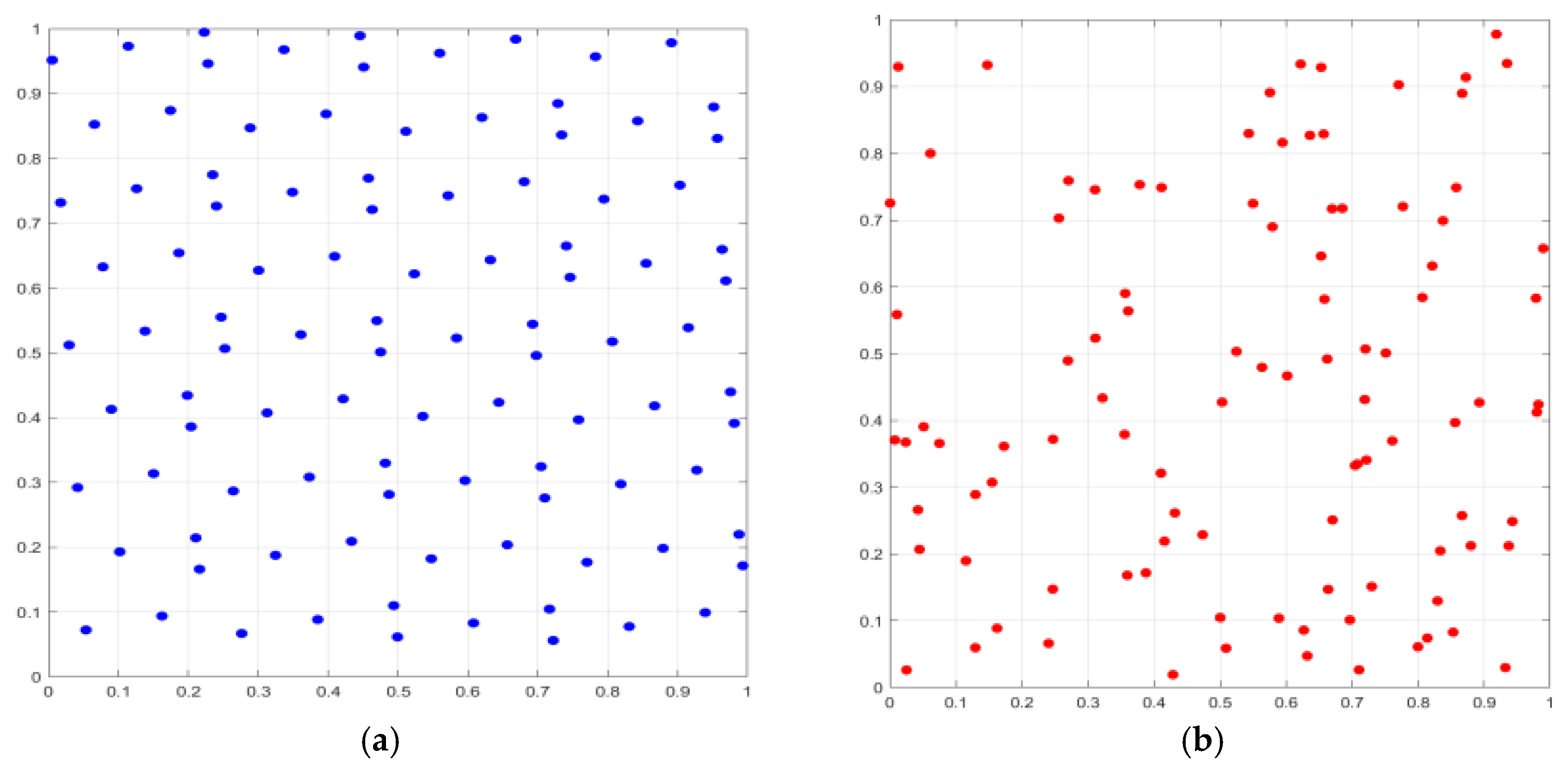
4.2.1. The Good Point Set Population Initialization

The SO uses the random initialization of the snake population, so the population distribution is random, resulting in the distribution of the entire solution space being difficult to be uniform, in some areas being very aggregated and in some areas being very dispersed, resulting in the algorithm’s utilization of the whole search space not being high and the diversity of the population not being strong. In this article, we adopt the strategy of the good point set to initialize the position of the snake population, and the distribution of the good point set can ensure a more balanced distribution in a multidimensional space, which solves the issue of the population’s unequal distribution. The optimal point set population initialization function is

$$\left\{\begin{array}{c}{P}_n\left(k\right)=\left(\left\{r_1^{\left(n\right)}\times k\right\},\left\{r_2^{\left(n\right)}\times k\right\},\cdots ,\left\{r_N^{\left(n\right)}\times k\right\}\right),1\le k\le n \\ \phi \left(n\right)=C\left(r,\epsilon \right)n^{-1+\epsilon } \\ r=2\mathit{cos}\left({\displaystyle \frac{2k\pi }{p}}\right),1\le k\le N \end{array}\right.$$

(22)

where $P_n\left(k\right)$ denotes the set of the good points, $\phi \left(n\right)$ denotes the deviation, $C\left(r,\epsilon \right)$ is a constant that only depends on$r,\epsilon$ and $\epsilon$ > 0, and $n$ is the number of points. $r$ denotes the good point, and $p$ denotes the minimum prime number that satisfies (23):

$${\displaystyle \frac{\left(p-3\right)}{2}}\ge N$$

(23)

Mapping it to the initialized search space is as follows:

$$X_i\left(t\right)=X_{min}+\left\{P_n\left(t\right)\right\}\times \left(X_{max}-X_{min}\right)$$

(24)

Compared to random initialization, the excellent point set initialization method is more efficient and equally distributed. In order to verify this point of view, in Figure 3, the comparison graph of the distribution of the population of the good point set and random initialization is set up in a two-dimensional space, and the number of populations is 100. It can be seen that compared with the good point set initialization in Figure 3a and the random initialization in Figure 3b, the population generated by the good point set initialization has a uniform distribution, which prevents it from falling into the local optimum, whereas the distribution of the population of random initialization is difficult to be uniform, which makes the algorithm prone to falling into the local optimum.

4.2.2. Fusion Particle Swarm Algorithm

Particle swarm optimization (PSO) is a population evolution-based optimization algorithm to simulate bird aggregation for foraging through particles [21]. Particles have two properties: velocity $V_i=\left[v_{i1},v_{i1}\cdots v_{id}\right]$ and position $X_i=[x_{i1},x_{i1}\cdots x_{id}]$. The positions of the particles in the search space represent potential solutions to the optimization problem in the particle swarm algorithm. In each iteration, the particle tracks two extremes to update its position and speed. The first one is the optimal solution $p_{best}$ found by the particle itself. The second is the current optimal solution $g_{best}$, for the entire particle swarm. After numerous iterations, the solution converges to the optimal solution. The velocity $v_{ij}$ and position $x_{ij}$ of particle $i$ in the $j$-dimension are updated using the following equation:

$$\left\{\begin{array}{c}{v}_{ij}\left(t+1\right)=\\ \omega v_{ij}\left(t\right)+c_1{r}_1\left(p_{besti}\left(t\right)-x_{ij}\left(t\right)\right)+c_2{r}_2\left(g_{best}\left(t\right)-x_{ij}\left(t\right)\right)\\ x_{ij}\left(t+1\right)=x_{ij}\left(t\right)+v_{ij}\left(t+1\right)\end{array}\right.$$

(25)

Since the convergence speed of the PSO is excellent, this study introduces it into the algorithm model to optimize the SO, with the aim of ensuring the search accuracy of the algorithm while improving its convergence speed. In the process of combining the snake algorithm and the particle swarm algorithm, the speed and position iteration formulas are updated as follows:

$$\left\{\begin{array}{c}{v}_{m,ij}\left(t+1\right)=\\ \omega v_{ij}\left(t\right)+c_1{r}_1\left(X_{best,m}-X_{i,m}\left(t\right)\right)+c_2{r}_2\left(X_{food}-X_{i,m}\left(t\right)\right)\\ X_{i,m}\left(t+1\right)=X_{i,m}\left(t\right)+v_{m,ij}\left(t+1\right)\end{array}\right.$$

(26)

$$\left\{\begin{array}{c}{v}_{f,ij}\left(t+1\right)=\\ \omega v_{ij}\left(t\right)+c_1{r}_1\left(X_{best,f}-X_{i,f}\left(t\right)\right)+c_2{r}_2\left(X_{food}-X_{i,f}\left(t\right)\right)\\ X_{i,f}\left(t+1\right)=X_{i,f}\left(t\right)+v_{f,ij}\left(t+1\right)\end{array}\right.$$

(27)

where $\omega ={\omega }_{max}-t\left({{\omega }_{max}-\omega }_{min}\right)/T$, ${\omega }_{max}=0.9,\mathrm{a}\mathrm{n}\mathrm{d}$ ${\omega }_{min}=0.6$.

4.2.3. Cauchy Variation Strategy

As female and male snakes search for food in the model, their range of movement in three-dimensional space decreases as the number of iterations increases, making it difficult for the snakes to jump out of the locally optimal solution, and thus making it difficult to reach the global optimum. To address this issue, this study proposes the use of the Cauchy variation strategy. Cauchy variation can jump out of the local optimal solution; the Cauchy distribution has a longer tail, which means it is easier to generate random values away from the mean so that the snake group can jump out of the local optimal solution, thus improving the performance of the algorithm. The Cauchy variation is a continuous probability distribution with a probability density function as follows:

$$f\left(x,x_0,r\right)={\displaystyle \frac{1}{\pi \gamma \left(1+{\left(\frac{x-x_0}{r}\right)}^2\right)}}$$

(28)

where $x$ is the variable, $x_0$ is the position parameter,$\mathrm{a}\mathrm{n}\mathrm{d} \gamma$ is the size parameter that determines the width of the distribution.

Setting γ to 1 leverages the symmetric heavy-tailed distribution characteristic of the probability density function, which effectively balances global exploration (escaping local optima) during convergence. As a result, in battle mode, each snake group individual’s position is updated as follows:

$$\left\{\begin{array}{c}{X}_{i,f}\left(i,j\right)=X_{i,f}\left(t\right)+Cauchy\left(\mathrm{0,1}\right)\ast X_{i,f}\left(t\right)\\ X_{i,m}\left(i,j\right)=X_{i,m}\left(t\right)+Cauchy\left(\mathrm{0,1}\right)\ast X_{i,m}\left(t\right)\end{array}\right.$$

(29)

where $Cauchy\left(\mathrm{0,1}\right)$ generates 1 Cauchy random number.

4.3. Improved Snake Algorithm Implementation Flow

To solve the premature convergence problem of the traditional snake algorithm in underwater path planning, this paper proposes to improve the snake algorithm ISO (see Algorithm 1 for details):

Algorithm 1: Improved snake algorithm pseudo-code (ISO).

STEP1. Modeling of obstacles, currents, and seabed.

STEP2. Using Equation (24), the population is initialized using the set of good points to generate N snakes (this strategy ensures that the initial solutions are uniformly distributed in the search space (Figure 3 compares the experiments), avoids the local aggregation problem caused by traditional random initialization, and lays the foundation for global convergence), 50% male and 50% female, to calculate the individual fitness as well as the best fitness of the male and female populations.

STEP3. While (t < T) do

STEP4. Evaluate each group ${ N}_m$ and ${ N}_f$

STEP5. The best female and male individuals $f_{best,f}, f_{best,m}$

STEP6. Use Equation (13) to define $Temp$, $Q$

STEP7. If (Q < 0.25)

Perform food search mode using Equations (26) and (27)

Else if (Q > 0.6)

Use Equation (16) to perform the movement to food mode

Else

If ($\mathrm{r}\mathrm{a}\mathrm{n}\mathrm{d}>0.6$)

Use Equation (29) to enter battle mode (the Cauchy variation strategy provides non-zero probability of jumping out of the local optimum through a heavy-tailed distribution)

Else

Use Equations (19) and (20) to enter mating mode

Using Equation (21) to change the position of the worst male and female snakes

End if

End if

End while

STEP8. Output optimal path

5. Simulation Experiment and Discussion

5.1. Hardware and Software Configuration

To verify the adequacy of the established model and the effectiveness of ISO, simulation experiments were performed under two types of underwater environment models, simple and complex. The three-dimensional routing effect of the ISO algorithm is then compared with JSO, ICFPSO, PSO, and SO. The computer simulation platform is MATLAB 2021b (parallel computing disabled to ensure fairness), the processor is an AMD Ryzen 7 4800H (8 cores, 16 threads, base frequency 2.9 GHz) is designed by Advanced Micro Devices (AMD) and headquartered in Santa Clara, California, United States, the running memory is 16.0 GB (3200 MHz), and the operating system is Windows 11-64b.

This study is based on the fact that the speed of the AUV is a constant value that is only affected by obstacles on the seabed and ocean currents, where the current flow rate is randomly generated by Equation (2).

5.2. Simulation Parameter Set

In the experiments of the simulation, the planning space was set as $1000 \mathrm{m}\times 1000 \mathrm{m}\times 300 \mathrm{m}$. The coordinates of the starting point were set as $\left[30;30;0\right],$ and the coordinates of the ending point were set as [900; 900; 150]. The effect of ocean currents on the AUV is not taken into account; the speed of the AUV is generally 0–10 $\mathrm{k}\mathrm{n}$ [22]. In this paper, the AUV is assumed to have a constant velocity of 3$\mathrm{m}/\mathrm{s}$ throughout the navigation process. The vortex parameters are $\Gamma$ = 10, $r_0$ = 1, $x_0=100$, and $y_0$ = 100, and the constant flow velocity is 0.5 $\mathrm{m}/\mathrm{s}$ [23].

Table 1. The algorithm parameters.

Algorithm	Parameter
ISO	$c_1=0.5,c_2=0.05,{\mathrm{c}}_3=2$ [20] ${\mathrm{V}}_{\mathrm{m}\mathrm{a}\mathrm{x}}=6,{\mathsf{\omega }}_{\mathrm{m}\mathrm{a}\mathrm{x}}=0.6,{\mathsf{\omega }}_{\mathrm{m}\mathrm{i}\mathrm{n}}=0.6$; [21]
JSO	$c_1=0.5,c_2=0.05,{\mathrm{c}}_3=2$; [20]
SO	$c_1=0.5,c_2=0.05,{\mathrm{c}}_3=2$; [20]
PSO	$c_1=2,c_2=2,{\mathsf{\omega }}_{\mathrm{m}\mathrm{a}\mathrm{x}}=0.9,$ [21] ${\mathsf{\omega }}_{\mathrm{m}\mathrm{i}\mathrm{n}}=0.6{,\mathrm{V}}_{\mathrm{m}\mathrm{a}\mathrm{x}}=6;$
ICFPSO	${\mathsf{\omega }}_{\mathrm{m}\mathrm{a}\mathrm{x}}=0.9,{\mathsf{\omega }}_{\mathrm{m}\mathrm{i}\mathrm{n}}=0.6,\mathsf{\sigma }=0.3$ $c_1=2.05,c_2=2.05;$ [19]
WOA	$\partial =1,\mathrm{p}=0.5;$ [24]

expresses the main parameters of the six algorithms. The initial population size $N$ is 50, the maximum number of iterations $T$ is 150, and the ISO, JSO, SO, PSO [21], ICFPSO [19], and WOA [24] are run 30 times each.

5.3. Analysis of Simulation Results

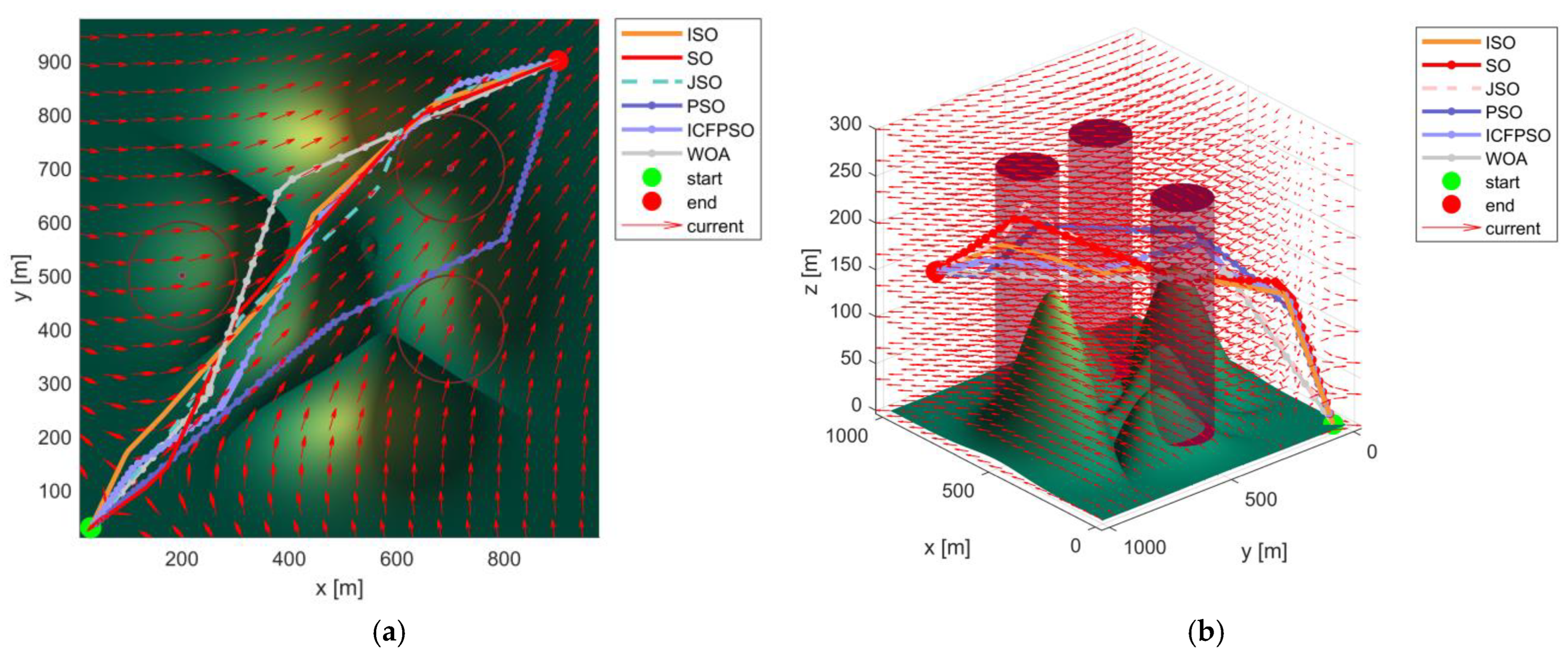
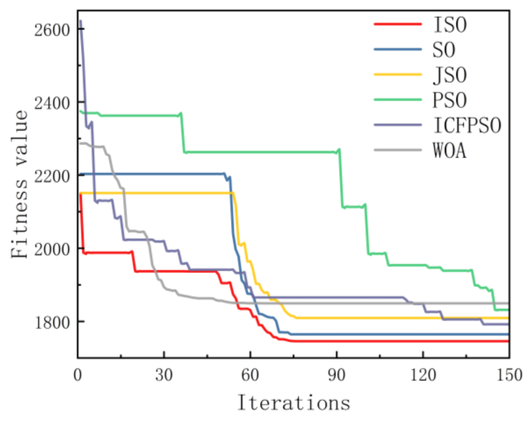
5.3.1. Simulation and Analysis in a Simple Underwater Environment

In this experiment, the maximum node of the path is set to five (excluding the two nodes of the start and end points).

Table 2. Obstacle coordinate position.

Obstacle	X-Axis	Y-Axis	Z-Axis	R-Radius
1	200	500	250	100
2	700	700	250	100
3	700	400	250	100

lists the locations of the three obstacle models. The path-planning outcomes of the ISO, SO, JSO, PSO, ICFPSO, and WOA algorithms are shown in Figure 4, and Figure 5 presents the graph of the fitness function.

In Figure 4, it can be seen that ISO generates the smoothest path with fewer transitions in simple environments, which matches the safe, energy-efficient, and effective path required by the AUV. On the adaptation curve comparison graph, it can be seen that ISO outperforms the other algorithms in terms of optimality finding, and there is an easy local optimum for PSO in the same experimental environment. The ICFPSO proposed in the literature no longer falls into a local optimum, but the finding accuracy is lower than PSO. WOA has a lower finding accuracy. Although SO can find the optimal value of the path, it easily falls into a long time of local optimality in the early stage. JSO, which is improved by the good point set, has a lower value than the SO algorithm at the beginning of the iteration, but like SO, it also falls into the local optimum in the early stage. ISO, which incorporates the PSO algorithm to improve the convergence speed and the Cauchy perturbation variant to improve the convergence accuracy, achieves better optimization accuracy and speed than the other algorithms. The following intricate underwater environment simulation experiments are carried out to further confirm the efficacy of the suggested improvement technique.

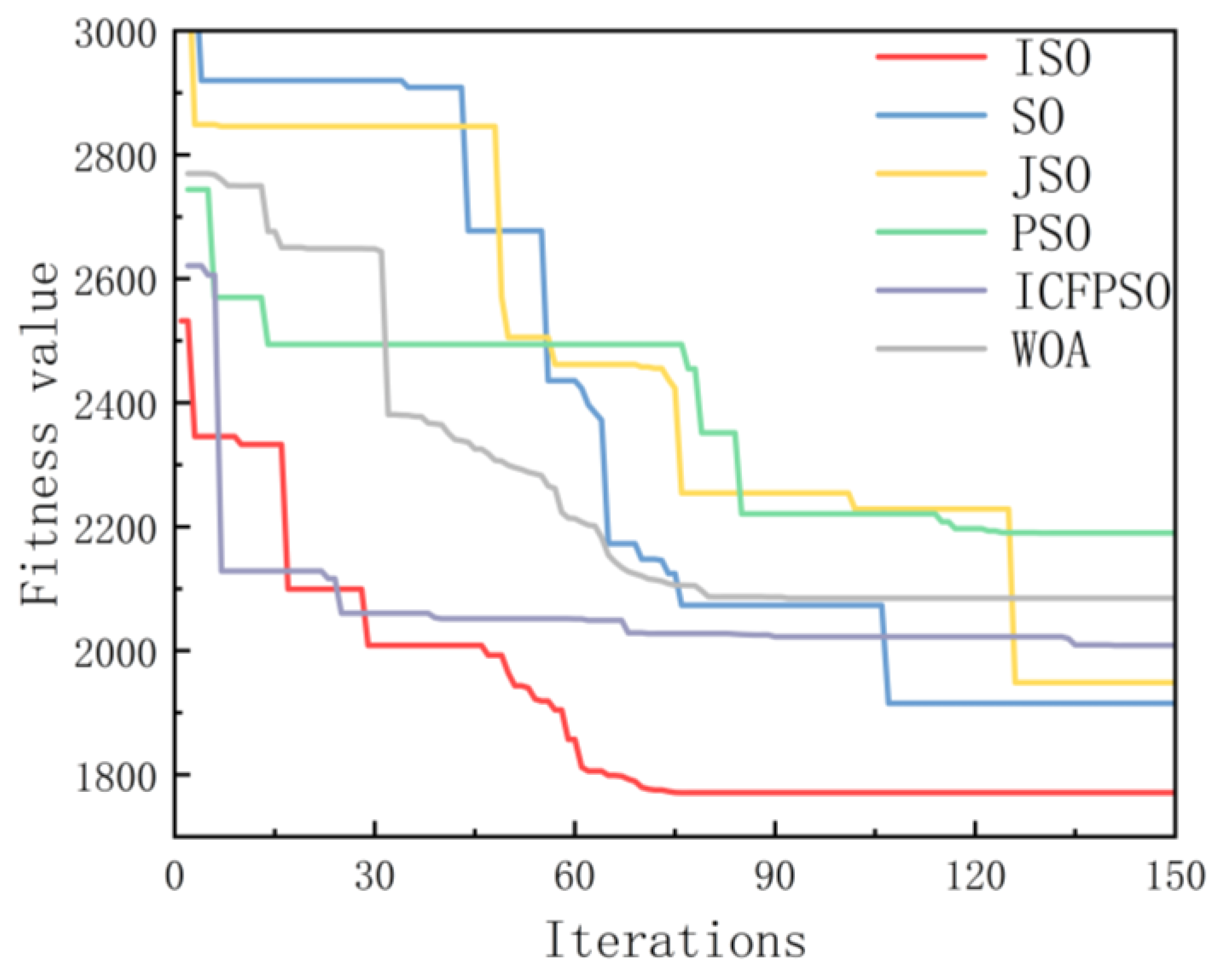
5.3.2. Simulation Analysis in Complex Environments

In this experiment, the maximum node of the path is set to ten (excluding the start and end points).

Table 3. Obstacle coordinate position.

Obstacle	X-Axis	Y-Axis	Z-Axis	R-Radius
1	200	450	250	80
2	300	700	250	80
3	350	200	250	80
4	500	350	250	80
5	600	200	250	80
6	650	750	250	80
7	700	550	250	80

lists the position of each obstacle model, Figure 6 displays the path-planning outcomes of the ISO, SO, JSO, PSO, ICFPSO, and WOA algorithms, and Figure 7 shows the graph of the fitness function

From Figure 6, it can be seen that the paths planned by SO and PSO have many twists and turns and are highly dangerous, and such paths are difficult to satisfy a reasonable AUV path. Except ISO, all other algorithms can find the end of the path, but the path redundancy is high; in comparison, the ISO algorithm is better than the other five algorithms, and the path planned by ISO is smoother, with fewer twists and turns and higher safety, which can satisfy the demand of an AUV path.

According to the adaptability graph of the complex underwater environment, PSO has the worst convergence accuracy; from the two-dimensional graph, it can be seen that it is due to too many turning points, and the path is not smooth enough. Overall, the ICFPSO proposed in the literature has the best convergence speed compared to PSO, SO, JSO, and WOA, but the convergence accuracy is slightly worse. ISO boasts the highest convergence accuracy in addition to the fastest convergence speed, which once again verifies the validity of the current improvement strategy.

5.4. Comparison of Path Performance Indicators

The decrease in the fitness value function reflects the actual effect of each algorithm in finding the optimal path, the decrease in the number of iterations directly reflects the convergence speed of the algorithms, and the standard deviation intuitively demonstrates the robustness of each algorithm.

From

Table 4. Simple underwater environmental performance index.

Algorithm	Iteration	Optimal Fitness Value	Bad Fitness Value	Average Fitness Value	Standard Deviation
ISO	74	1746.0071	1851.4202	1782.7790	25.0002
SO	74	1764.6845	2026.2010	1912.3748	88.8609
JSO	76	1809.4664	1951.4591	1860.2239	38.3603
PSO	145	1831.6363	2290.7304	1999.8093	119.2672
ICFPSO	141	1792.0699	2286.7562	1961.4648	123.5316
WOA	84	1849.3287	2291.2009	2014.4558	103.2262

, it can be seen that in simple underwater environments, the average fitness values of the ISO algorithm are improved by 7.2% and 4.3% over the SO and JSO algorithms, respectively, while compared to PSO, ICFPSO, and WOA, they are improved by 12%, 10%, and 12%, respectively. In terms of the number of iterations, both the ISO and SO algorithms converged within 74 iterations, but ISO achieved better fitness values than the other algorithms in each optimization, indicating that ISO can effectively reduce the navigation cost and achieve path optimization in path planning. In the third evaluation metric (standard deviation), ISO has the smallest standard deviation, which is reduced by 63.86 and 13.36 compared to SO and JSO, respectively, and 94.27, 98.53, and 78.226 compared to PSO, ICFPSO, and WOA, respectively, which indicates that ISO is more stable and robust in path planning.

In complex underwater environments, the path-planning advantage of the ISO algorithm is more obvious, as can be seen in

Table 5. Complex underwater environment performance index.

Algorithm	Iteration	Optimal Fitness Value	Bad Fitness Value	Average Fitness Value	Standard Deviation
ISO	74	1771.1727	2140.1336	1987.4769	83.4097
SO	107	1915.0162	2494.3869	2186.5361	121.6212
JSO	126	1948.7345	2474.9318	2165.5661	145.8995
PSO	144	2189.8619	3067.4882	2557.2128	257.9741
ICFPSO	141	2008.7076	3031.5748	2371.4958	240.4899
WOA	115	2084.6708	3091.9430	2438.1219	242.4011

. The average fitness values of ISO are improved by 10% and 8.9% compared to SO and JSO, respectively, and by 28.67%, 19.32%, and 22.67% compared to PSO, ICFPSO, and WOA, respectively. ISO still maintains its convergence within 74 iterations, and its optimal fitness value is significantly lower than the other algorithms. In terms of standard deviation, ISO is reduced by 38.21 and 62.49 compared to SO and JSO, and by 174.56, 157.08, and 158.99 compared to PSO, ICFPSO, and WOA, respectively.

In summary, ISO satisfies the path-planning requirements of AUVs in terms of path smoothness, path quality, and path-planning efficiency and shows strong exploration and development capabilities, achieving faster convergence speed and higher optimization accuracy, as well as good robustness. These advantages make ISO an effective solution for complex underwater path-planning problems.

6. Conclusions

This study investigates the problem of AUV path planning in a complex underwater environment model that takes into account the effects of distance, currents, obstacles, and navigational altitude. The underwater environment model is established by simulating the underwater conditions, and the objective function of optimal fitness is established and transformed into a multi-objective constraint function optimization problem.

The proposed ISO algorithm solves the problem that SO easily falls into the local optimum, accelerates convergence speed and optimality finding accuracy, and improves robustness. In the simulation experiments, two mission scenarios of simple and complex underwater environments are considered, and the proposed algorithm can successfully cope with different underwater environments for the conditions used. By comparison with other algorithms, the effectiveness and practicality of ISO are verified for the environments considered. The results of the simulation demonstrate that ISO can generate safe, low-energy, and path-optimal AUV navigation planning, which is better than other comparative algorithms, verifying its effectiveness and practicality.

The successful validation of the static model lays the foundation for the subsequent introduction of dynamic data. In the future, a time-varying ocean current module can be embedded in the ISO framework, or the adaptation function can be updated with real-time data.

References

1. Hwang, J.; Bose, N.; Fan, S. AUV Adaptive Sampling Methods: A Review. Appl. Sci. 2019, 9, 3145. [Google Scholar] [CrossRef]
2. Wang, C.; Mei, D.; Wang, Y.; Yu, X.; Sun, W.; Wang, D.; Chen, J. Task Allocation for Multi-AUV System: A Review. Ocean Eng. 2022, 266, 112911. [Google Scholar] [CrossRef]
3. Cheng, C.; Sha, Q.; He, B.; Li, G. Path Planning and Obstacle Avoidance for AUV: A Review. Ocean Eng. 2021, 235, 109355. [Google Scholar] [CrossRef]
4. Kulkarni, C.S. Three-Dimensional Time-Optimal Path Planning in Dynamic and Realistic Environments; Massachusetts Institute of Technology: Cambridge, MA, USA, 2017. [Google Scholar]
5. Hai-Feng, J.; Yu, C.; Wei, D.; Shuo, P. Underwater Chemical Plume Tracing Based on Partially Observable Markov Decision Process. Int. J. Adv. Robot. Syst. 2019, 16, 1729881419831874. [Google Scholar] [CrossRef]
6. Taheri, E.; Ferdowsi, M.H.; Danesh, M. Closed-Loop Randomized Kinodynamic Path Planning for an Autonomous Underwater Vehicle. Appl. Ocean Res. 2019, 83, 48–64. [Google Scholar] [CrossRef]
7. Yan, S.; Pan, F. Research on Route Planning of AUV Based on Genetic Algorithms; IEEE: Piscataway, NJ, USA, 2019; pp. 184–187. [Google Scholar]
8. MahmoudZadeh, S.; Powers, D.M.; Yazdani, A.M.; Sammut, K.; Atyabi, A. Efficient AUV Path Planning in Time-Variant Underwater Environment Using Differential Evolution Algorithm. J. Mar. Sci. Appl. 2018, 17, 585–591. [Google Scholar] [CrossRef]
9. Lim, H.S.; Fan, S.; Chin, C.; Chai, S.; Bose, N. Particle Swarm Optimization Algorithms with Selective Differential Evolution for AUV Path Planning. Int. J. Robot. Autom. 2020, 9, 94–112. [Google Scholar] [CrossRef]
10. Che, G.; Liu, L.; Yu, Z. An Improved Ant Colony Optimization Algorithm Based on Particle Swarm Optimization Algorithm for Path Planning of Autonomous Underwater Vehicle. J. Ambient Intell. Humaniz. Comput. 2020, 11, 3349–3354. [Google Scholar] [CrossRef]
11. Cao, X.; Sun, H.; Guo, L. Potential Field Hierarchical Reinforcement Learning Approach for Target Search by Multi-AUV in 3-D Underwater Environments. Int. J. Control 2020, 93, 1677–1683. [Google Scholar] [CrossRef]
12. Havenstrøm, S.T.; Rasheed, A.; San, O. Deep Reinforcement Learning Controller for 3D Path Following and Collision Avoidance by Autonomous Underwater Vehicles. Front. Robot. AI 2021, 7, 566037. [Google Scholar] [CrossRef] [PubMed]
13. Liang, Z.; Qu, X.; Zhang, Z.; Chen, C. Three-Dimensional Path-Following Control of an Autonomous Underwater Vehicle Based on Deep Reinforcement Learning. Pol. Marit. Res. 2022, 29, 36–44. [Google Scholar] [CrossRef]
14. MathWorks, MATLAB; Version R2021b; The MathWorks, Inc.: Natick, MA, USA, 2021.
15. Garau, B.; Alvarez, A.; Oliver, G. AUV Navigation Through Turbulent Ocean Environments Supported by Onboard H-ADCP; IEEE: Piscataway, NJ, USA, 2006; pp. 3556–3561. [Google Scholar]
16. Zhang, S.; Nie, Y.; Wang, S.; Zhang, X.; Wu, Q.; Wang, T. 3-D Path Planning for AUVs Based on Improved Exponential Distribution Optimizer. IEEE Internet Things J. 2024, 11, 28667–28679. [Google Scholar] [CrossRef]
17. Sun, Y.; Luo, X.; Ran, X.; Zhang, G. A 2D Optimal Path Planning Algorithm for Autonomous Underwater Vehicle Driving in Unknown Underwater Canyons. J. Mar. Sci. Eng. 2021, 9, 252. [Google Scholar] [CrossRef]
18. Mu, X.; Gao, W. Coverage Path Planning for Multi-AUV Considering Ocean Currents and Sonar Performance. Front. Mar. Sci. 2025, 11, 1483122. [Google Scholar] [CrossRef]
19. Li, X.; Yu, S. Three-Dimensional Path Planning for AUVs in Ocean Currents Environment Based on an Improved Compression Factor Particle Swarm Optimization Algorithm. Ocean Eng. 2023, 280, 114610. [Google Scholar] [CrossRef]
20. Hashim, F.A.; Hussien, A.G. Snake Optimizer: A Novel Meta-Heuristic Optimization Algorithm. Knowl.-Based Syst. 2022, 242, 108320. [Google Scholar] [CrossRef]
21. Marini, F.; Walczak, B. Particle Swarm Optimization (PSO). A Tutorial. Chemom. Intell. Lab. Syst. 2015, 149, 153–165. [Google Scholar] [CrossRef]
22. Yanan, L.; Haibin, H.; Liangming, C.; Yufei, Z.; Xiaoli, W. Energy-Optimal Three-Dimensional Path Planning for AUV under Changing Ocean Current Environment. Syst. Eng. Electron. 2021, 43, 3667. [Google Scholar]
23. Zhou, H.; Wang, H. Research on Path Planning of Unmanned Underwater Vehicle for Long-Duration Missions Based on Energy Consumption Optimization in Complex Ocean Environments; Harbin Engineering University: Harbin, China, 2017. [Google Scholar]
24. Mirjalili, S.; Lewis, A. The Whale Optimization Algorithm. Adv. Eng. Softw. 2016, 95, 51–67. [Google Scholar] [CrossRef]
Figure 1. Three-dimensional complex seafloor model.
Jmse 13 00796 g001
Figure 2. AUV sailing altitude diagram.
Jmse 13 00796 g002
Figure 3. Comparison of the distribution of the optimal point set and the randomly initialized population. (a) The good point set population initialization distribution simulation diagram. (b) The random initialization set population initialization distribution simulation diagram.
Jmse 13 00796 g003
Figure 4. The algorithms are compared in a simple underwater environment. (a) Simple underwater environmental path-planning two-dimensional simulation diagram. (b) Simple underwater environment path-planning three-dimensional simulation diagram.
Jmse 13 00796 g004
Figure 5. Comparison of fitness curves of different algorithms in a simple underwater environment.
Jmse 13 00796 g005
Figure 6. The path comparison of each algorithm in a complex underwater environment. (a) Complex underwater environment path-planning two-dimensional simulation diagram. (b) Complex underwater environment path-planning three-dimensional simulation diagram.
Jmse 13 00796 g006
Figure 7. Comparison diagram of the fitness curves of various algorithms in a complex underwater environment.
Jmse 13 00796 g007