Risk–Failure Interactive Propagation and Recovery of Sea–Rail Intermodal Transportation Network Considering Recovery Propagation

Abstract

Existing research concentrates on analyzing the propagation and recovery of complex network risk or failure under a single model, which makes it difficult to effectively deal with the chain reaction. Concerning the recovery delay caused by the risk–failure interactions, this paper proposes a model for the propagation and recovery of risk–failure interactions. This model not only considers the network risk–failure interactive propagation mechanism but also introduces the load-balancing strategy and repair mechanism. The study quantifies the impact of the station on network resilience after different attack modes. In addition, the resilience metrics based on the station failure are established to accurately represent the resilience evolution of the network during propagation and recovery. Finally, focusing on the Belt and Road transportation network, we explore the evolution of network resilience under the variation of failure station repair time, station risk state recovery rate, and hub station allocation parameters. The simulation results showed that the model reduced the resilience loss through resilience recovery and accelerated the network back to normal in the face of attacks, shortening the station repair time and increasing the station risk recovery rate significantly improved the overall resilience level of the network, and increasing the proportion of hub station balancing based on the residual capacity effectively improved the minimum resilience of the sea–rail intermodal transportation network.

1. Introduction

With the continuous growth of international trade and logistics demands, the scale of the sea–rail intermodal transportation network has been expanding significantly. As core hubs within the international logistics system, seaports and railway networks have evolved into critical infrastructure, underpinning global supply chains and facilitating coordinated regional economic development [1,2]. In recent years, intensive transportation network construction has enhanced the linkage efficiency between seaports and inland railway hub stations, with cargo transfer efficiency between these two transportation modes demonstrating significant improvement. Through container standardization and technological innovations in intermodal transportation, seaports and railway networks have established a deeply integrated three-dimensional transportation system [3,4].

However, the sea–rail intermodal transportation system faces multiple operational risks, including extreme weather disasters, geopolitical conflicts, and cybersecurity threats [5,6]. When a hub station experiences operational suspension due to typhoons or equipment failure, cargo transfer demand shifts to neighboring stations, resulting in container yards exceeding their designed capacity. Given the capacity constraints of railway branch lines, the associated inland transportation networks may trigger cascade effects, potentially inducing systemic risks, including cargo backlog and scheduled freight train delays [7]. Such dynamically propagating transportation disruptions may undermine the stability of regional industrial chains, thereby affecting international trade patterns.

Following major disruption events, the sea–rail intermodal transportation system requires the implementation of intelligent recovery strategies [8]. For damaged stations’ restoration and reactivation, it necessitates not only the recovery of local loading/unloading capacity but also the reconfiguration of scheduled freight train resources through dynamic scheduling algorithms. During this process, certain stations may experience processing delays due to temporary task surges, which can be further mitigated through real-time route optimization. By establishing resilience recovery mechanisms, transportation networks can achieve step-wise transport capacity rebalance, ultimately restoring network resilience [9,10]. Leveraging the synergistic characteristics of intermodal networks, complex network theory has been extensively applied to deconstruct the hierarchical topological structure of sea–rail intermodal transportation systems, establishing a quantitative analytical framework for evaluating network resilience under disruptive events [11]. The sea–rail intermodal transportation system can be modeled as a dual-layer network composed of coastal station clusters, inland railway freight stations, maritime shipping routes, and railway trunk lines.

Numerous scholars have conducted extensive research on risk propagation and cascade failure in complex networks. Regarding risk propagation, studies have employed frameworks, such as the epidemic model Susceptible-Exposed-Infectious-Recovered (SEIR) and its modified derivatives [12,13,14]. In cascade failure modeling, representative approaches, such as the ORNL-PSerc-Alaska (OPA) model and load-capacity models, have been developed to characterize failure propagation within networks [15,16]. These research findings have been widely applied to single-mode transportation networks, such as maritime shipping networks and railway networks. However, in practical scenarios, risk propagation and failure propagation coexist simultaneously and cannot be described using single risk or failure propagation models. Previous works treated risk and failure as distinct phenomena. The interactive propagation of risk–failure is ignored, i.e., risk will lead to failure, and further failure will lead to new risk. At the same time, most of the previous studies have only considered the recovery propagation in the transportation network from the perspective of a single-layer network.

In view of the above issues, considering the spread of risk–failure and recovery processes, this study aims to address the gaps in existing risk–failure propagation models by achieving the following objectives:

(1)

In view of the problem that the network risk–failure interactive propagation problem has not been considered in previous studies, a risk regression and failure propagation mechanism with an interactive propagation mechanism is proposed.

(2)

The proposed resilience recovery model refines the station risk–failure dynamics by introducing a risk recovery mechanism, a load-balancing strategy, and a repair mechanism. In addition, it establishes resiliency metrics based on the severity of station failure.

(3)

To study the effectiveness of the model, an empirical study is conducted on the multimodal transport network of the Belt and Road Initiative. Through multi-scenario simulation experiments, the resilience changes of the sea–rail multimodal transport network under the hybrid attack mode are systematically analyzed.

2. Related Works

The impacts of disasters and accidents on networks typically manifest in two forms: risk and failure. Risk refers to the potential negative consequences arising from uncertainties within specific environmental and temporal contexts. In complex networks, risk propagation denotes the dynamic process through which risk (e.g., financial risk, diseases, and rumors) diffuses via nodes and connections within the network [17,18]. To investigate the evolutionary mechanisms of risk propagation in complex networks, scholars have implemented this framework in practical network systems, such as supply chain networks, multimodal transportation networks, and industrial systems. Liang et al. integrated complex networks with epidemic models to examine the structural impacts of risk propagation on global supply networks [19]. He et al. introduced cascade failure theory into risk propagation analysis of multimodal transportation networks, elucidating intrinsic patterns of risk diffusion [20]. Lyu et al. analyzed the interactions among flow dynamics, risk, and ripple effects within binary supply–demand relationships at transport nodes [21]. Shi et al. developed a quantitative risk analysis method combining complex networks with the Decision-Making Trial and Evaluation Laboratory (DEMATEL) to investigate risk evolution following ship collision accidents [22]. Feng et al. applied epidemiological models to study risk propagation in complex industrial systems, revealing accident risk propagation mechanisms [23]. Li et al. employed effective transfer entropy to construct container ship delay propagation risk networks, exploring latent propagation mechanisms of delay risk [24].

Failure occurs when disasters strike a network, causing compromised operational performance of nodes [25,26]. Node failure propagation directly induces performance degradation across the entire network, potentially culminating in systemic paralysis [27]. To quantify the impacts of failure propagation on complex networks, scholars have conducted targeted investigations through specialized modeling approaches. Zhang et al. investigated the robustness of urban rail transit networks against cascade failure induced by passenger flow fluctuations under various failure modes [28]. Xu et al. proposed a novel global liner shipping network cascade failure model, incorporating real-world factors of port rotation adjustments during port disruptions [29]. Lu et al. developed an enhanced coupled map lattice model to simulate the evolution process of chain failure in rail transit networks, quantifying critical influencing factors of cascade failure [30]. Huang et al. analyzed the vulnerability of hazardous material transportation networks under intentional-attack-induced cascade failure. Duan et al. established a two-stage cascade failure model to observe traffic congestion evolution patterns based on route selection behaviors [31].

In addressing the mitigation of node failure impacts in networks, scholars have developed strategies focusing on node self-recovery mechanisms and network edge augmentation to reduce failure severity. Jing et al. constructed a cascade failure model with time-delay characteristics by incorporating temporal lags in failure propagation, proposing node recovery probabilities during cascade processes to enhance the robustness of coupled networks [32]. Li et al. introduced weak connections and diverse disruption scenarios into cascade failure propagation to analyze network resilience [33]. Li et al. accounted for node load heterogeneity in cascade failure and proposed a resilience reinforcement strategy based on node capacity redundancy, examining network resilience evolution through coupled failure–recovery processes [34]. Lu et al. employed a modified disaster spreading theory model to simulate dynamic origin–destination demand shifts under disruptions, time-delayed cascade effects, and their interactions with spatiotemporal passenger flow heterogeneity, effectively reducing cascade failure scales through directional flow heterogeneity utilization [35]. Guo et al. pioneered the integration of recovery propagation concepts into metro-bus bilayer network cascade failure modeling, establishing novel theoretical perspectives for urban transportation network resilience analysis and recovery strategies [36].

While the aforementioned studies have achieved notable advancements in modeling node dynamic propagation and recovery mechanisms, traditional static protection mechanisms increasingly reveal limitations in addressing the growing openness and dynamicity of complex transportation networks. These conventional approaches exhibit inherent lags in system maintenance responses, with sole reliance on local node repair or topological optimization proving inadequate to counter systemic risk triggered by sudden disturbances. Within this context, resilience theory provides a more inclusive analytical framework by integrating system response characteristics across early, middle, and late phases, enabling the revelation of dynamic propagation thresholds for network failure, recovery path selection mechanisms, and their coupling relationships with system structural functionalities [37]. The tri-phase synergistic mechanism of “resistance–adaptation–recovery” embedded in resilience theory represents a methodological breakthrough for quantifying evolutionary patterns of transportation systems throughout disturbance cycles [38]. Fan et al. proposed a degree deviation-based enhanced connectivity link addition method to maintain multiplex network resilience [39]. Liu et al. developed graph-theoretic topological metric-based resilience measurements to assess European port network resilience under three potential attack strategies [40]. Cao et al. created a pioneering resilience analysis framework for cascade failure through examining port betweenness, weight, and connectivity impacts on load determination and target selection, systematically investigating port disruption effects on maritime network resilience [41]. Dong et al. implemented connection quality thresholds to quantify network resilience metrics, with varying link quality threshold sensitivities reflecting urban transportation network resilience characteristics [42]. Yin et al. developed an integrated model to evaluate critical infrastructure service levels of urban transportation under diverse disruptions for quantifying network resilience [43]. Bai et al. proposed a cascade reaction simulation model with locally weighted flow redistribution rules to assess dynamic resilience in global liner shipping networks [44]. Xu et al. introduced a dynamic cascade failure model incorporating port rotation adjustments and liner service routing behaviors during port failure to mitigate congestion [29]. Chen et al. investigated topological and service characteristic measurements of intercity public transportation subnetworks and multimodal networks under heterogeneous disruptions [45]. Zhou et al. established a cost-based generalized evaluation system considering heterogeneous freight demands to quantify the resilience of China–Europe integrated freight networks across multiple disruption scenarios [46].

Current research has achieved substantial progress in risk propagation, failure propagation, and resilience. However, based on the aforementioned literature analysis, existing studies still present the following issues: (1) Most current studies focus on isolated risk or failure propagation, neglecting the impact of risk–failure interactive propagation on network performance. (2) Existing research lacks network resilience analysis under risk–failure interactive propagation and recovery mechanisms. (3) Few studies investigate post-disruption recovery propagation in transportation networks from a dual-layer network perspective.

In view of the above problems, the main contributions of this paper are as follows:

(1)

To address the incomplete assessment of network risk–failure interaction causing recovery delays, this research breaks through the limitations of traditional single risk or failure propagation models. We propose a risk backward and failure forward propagation mechanism with interactive propagation mechanisms to quantify risk–failure interaction propagation and recovery dynamics in networks.

(2)

The proposed resilience recovery model focuses on refining the extent of station risk–failure, introducing a risk recovery mechanism, load-balancing strategy, and repair mechanism. Additionally, a resilience metric based on station failure severity is established to accurately represent the evolutionary process of network resilience during propagation and recovery.

(3)

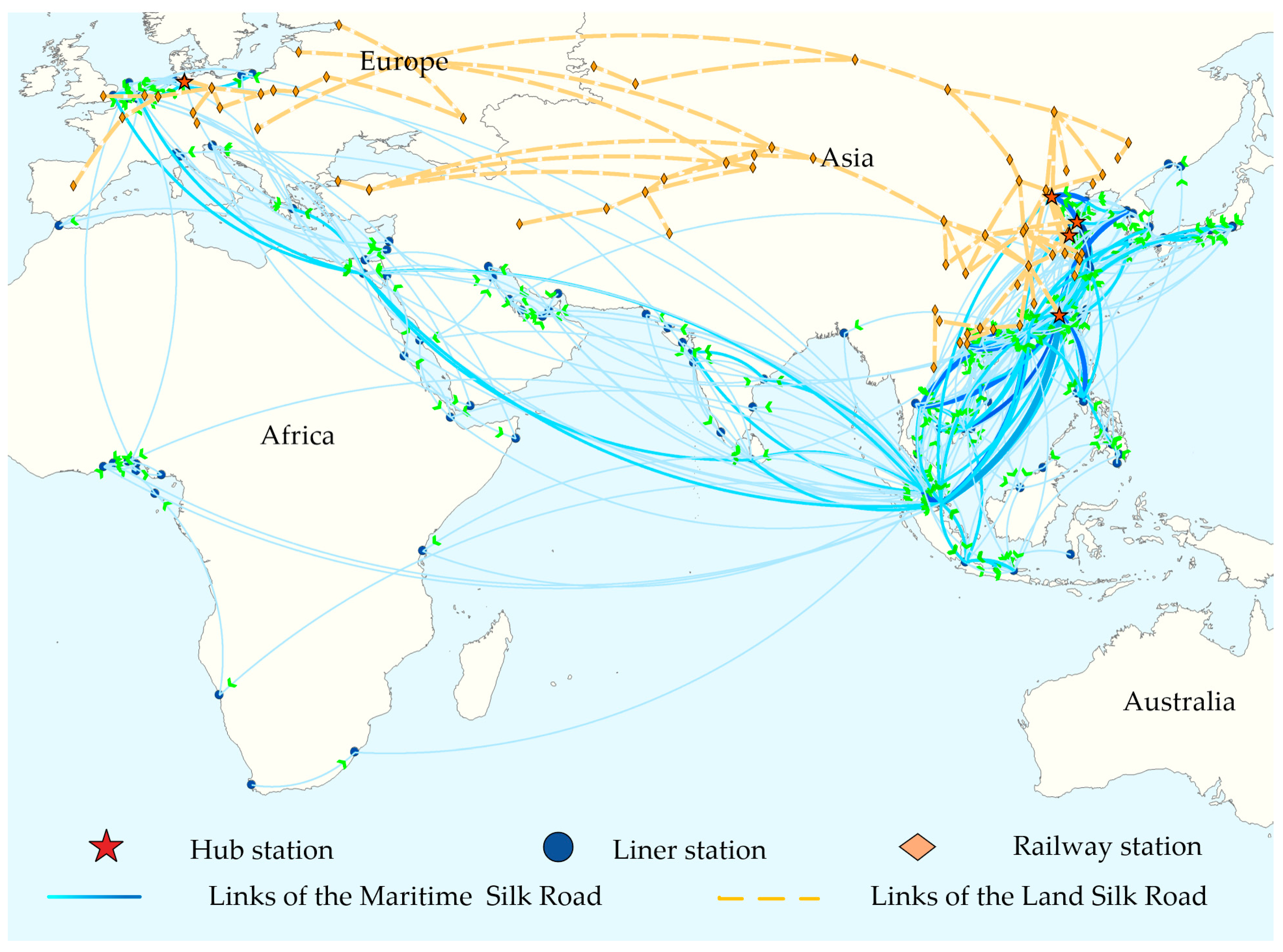
This paper conducts empirical research on the Belt and Road multimodal transportation network. Characterized by cross-regional and multimodal features, this network provides an ideal scenario for validating risk–failure interactive propagation and recovery mechanisms. Through multi-scenario simulation experiments, we systematically analyze resilience variation in the sea–rail intermodal transportation network under hybrid attack modes, focusing on three dimensions: repair capacity adjustment, risk management, and hub station allocation equalization. Simulation results offer scientific evidence for enhancing transportation network safety.

3. Method

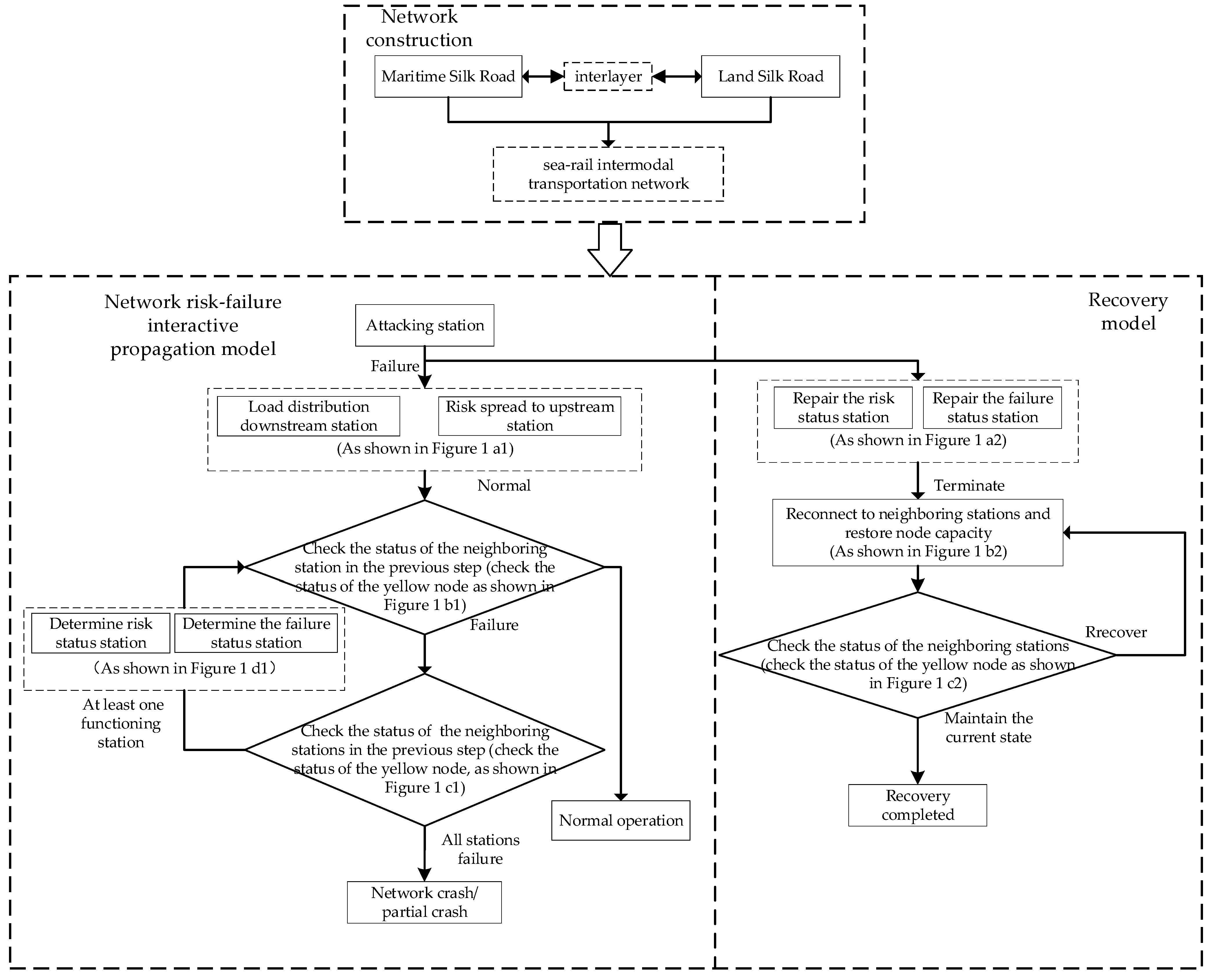
3.1. Risk–Failure Interactive Propagation and Recovery

When a network station is attacked, part of the infrastructure may be destroyed to become a failure station. This leads to the risk of backlogs at upstream stations because they cannot continue to transport loads to the failure station. At the same time, the load from the failure station needs to be redistributed to the downstream station, which further increases the transportation pressure and significantly reduces the transportation efficiency, thus triggering the interactive propagation of network risk–failure. In the process, the failure station also needs to take measures to restore network resilience. The above process is called the risk–failure interactive propagation and recovery mechanism of the transportation network.

The transportation network studied in this paper consists of two kinds of transportation routes, liner and railway, forming a sea–rail intermodal transportation network. In this paper, the stations are divided into hub stations and non-hub stations according to whether they can support the two modes of transportation. Among them, the hub station can be used as both a liner and railway station, while the non-hub station can only be used as a liner or railway station. In order to illustrate the risk–failure interactive propagation and recovery mechanism in the transportation network, this section takes the attacking hub station as an example, and the specific flow of risk–failure interactive propagation and recovery in the sea–rail intermodal transportation network is shown in Figure 1.

The process of risk–failure interactive propagation and recovery in the transportation network can be divided into the following stages.

First, as shown in Figure 1(a1), when hub station E was attacked, the station failed and was marked as red, and its load was redistributed to downstream liner station H and railway station F, while the risk spread upstream to liner station D and railway station G. The rule for this redistribution is summarized in Section 3.3.2.

Subsequently, the neighboring liner stations, D and H, and railway stations, G and F, of the failure station were checked, and their status was marked in yellow, as shown in Figure 1(b1). If some of the neighboring liner stations, D and H, and railway station, F, failed, as shown in Figure 1(c1), the station was marked in orange and the load was redistributed to the downstream liner stations, I and J, and railway station, L, while the risk continued to propagate upstream to liner stations A and B. The risk was then redistributed to the downstream liner stations, I and J, and railway station, L. At this stage, liner stations A, B, I, and J and railway station L were marked yellow to check their status, as shown in Figure 1(d1).

In the process of risk–failure spreading, once the hub station E was back to normal, it was marked green, as shown in Figure 1(a2). Meanwhile, the yellow marker was used to check the status of the neighboring liner stations D and H and railway stations G and F. If the neighboring liner stations, D and H, and railway station, F, were also back to normal, as shown in Figure 1(b2), the transportation routes with the neighboring stations were repaired.

Finally, as shown in Figure 1(c2), stations D, H, and F, which were restored to normal status, checked the status of their neighboring liner stations A, B, I, and J and liner station L and marked their status using yellow color.

In this process, the transportation route was restored after the transportation function of the station was also restored. As propagation and recovery evolved, the station recovered from or avoided a failure, which in turn facilitated dynamic risk–failure propagation and recovery across the network.

3.2. Model Assumptions

Assumption 1: 

The transportation network stations have a safety threshold. Stations can handle the impacts of internal and external environments within this threshold. If the impact exceeds this threshold, the station will face failure.

Assumption 2: 

Stations have the ability to repair risk. When affected by risk, stations can mitigate the negative impacts of risk through the recovery mechanism.

Assumption 3: 

According to the different extents of station failure, they can be divided into normal stations, complete failure stations, and partial failure stations.

3.3. Risk–Failure Interactive Propagation and Recovery Model

Based on the risk–failure interactive propagation and recovery mechanism, this paper constructed a network risk–failure interactive propagation and recovery model. The model was constructed with three main parts: network construction, network risk–failure interactive propagation model, and recovery model. The model framework is shown in Figure 2. The commonly used mathematical symbols in the text are shown in

Table 1. Mathematical symbols in frequent notation.

Symbol	Type	Description	Symbol	Type	Description
$S$	State	Node $i$ is in a susceptible state	${\vartheta }_i$	Parameter	The station $i$ additional load capacity
$D$	State	Node $i$ is in a dangerous state	$C$	Parameter	Hybrid attack
$I$	State	Node $i$ is in an infectious state	${\tau }_{FFC}$	Parameter	The failure propagation rate
$R$	State	Node $i$ is in a recovered state	$\zeta$	Parameter	The propagation interaction coefficient
$C_1$	Parameter	Degree attack	$d_i^{in}$	Parameter	The in-degree value of a station $i$ in the network
$C_2$	Parameter	Betweenness attack	${\mu }_Y\left(t\right)$	Parameter	Network failure intensity rate based on the node failure state $Y$
$C_3$	Parameter	Closeness attack	${\Psi }_Y\left(t\right)$	Parameter	Network maximum connectivity rate based on the node failure state $Y$
$\lambda$	Parameter	Node state conversion rate	$E(t)$	Parameter	Network efficiency
${\sigma }_{st}$	Parameter	The total number of shortest paths from the station $s$ to the station $t$	${\phi }_i\left(t\right)$	Parameter	Load of partial failure node $i$ at time $t$
$d\left(i,j\right)$	Parameter	The length of the shortest path from the station $i$ to the station $j$	${\mho }_i$	Parameter	The out-degree scale factor
$\Delta W_{FFC}^{i\to M_q}\left(t\right)$	Intermediate variables	The load increment distributed from the hub station $i$ to its neighboring stations $M_q$ at the time $t$	${\mathrm{{\rm Z}}}_i$	Function	The functional relationship between the station failure state function $Y_i$
$M_q$	Function	The functional station set of the neighboring stations $q$ of the hub station $i$	$M_1$	Set	Set of normal nodes
$\Delta W_{FFC}^{i\to j}\left(t\right)$	Intermediate Variables	The load increment distributed from the non-hub station $i$ to its neighboring stations $j$ at time $t$	$M_2$	Set	Set of partial failure nodes
${\tau }_{BRP}$	Parameter	Backward risk propagation rate	$M_3$	Set	Set of complete failure nodes
$T$	Decision variables	The station repair time	$M$	Set	Set of nodes
${\lambda }_3$	Decision variables	The station risk state recovery rate	$\theta$	Decision variables	The load redistribution parameter based on residual capacity
${\Gamma }_p\left(t\right)$	Set	The set of neighboring stations for the risk recovered status station $p$	$\vartheta$	Decision variables	A load redistribution parameter based on the intermediary strength

.

3.3.1. Attack Mode

To ensure the normal operation of liner, railway, and hub stations in the sea–rail intermodal double-layer network, at the initial moment $t_0$ in the network model, the station $i$ capacity $A_i\left(t_0\right)$ is linearly related to the initial load $W_i\left(t_0\right)$ of the network station, which are defined as follows:

$$A_i\left(t_0\right)=\left(1+{\vartheta }_i\right)W_i\left(t_0\right),$$

(1)

where ${\vartheta }_i$ represents the station $i$ additional load capacity, ${\vartheta }_i$> 0, which is a parameter that can be adjusted to meet the station’s varying load requirements across different scenarios.

In this attack mode, the network model combines different attack methods to launch a hybrid attack on the stations, in order to more effectively disrupt the structure and function of the transportation network. As the number of attacks increases, different attack modes will act randomly, gradually weakening the overall resilience level of the network. The hybrid attack mode $C$ designed in this paper includes three single-attack modes, denoted as $C_1$,$C_2$,and $C_3$, which are defined as follows:

$$F\left(i,C\right)=\left\{\begin{array}{c}{k}_i,C=C_1\\ {\displaystyle \sum _{s\ne i\ne t}\frac{{\sigma }_{st}\left(i\right)}{{\sigma }_{st}},C=C_2}\\ {\displaystyle \sum _{j\in M}\frac{1}{d\left(i,j\right)},C=C_3}\end{array}\right.,$$

(2)

where, when $C=C_1$, the attack mode adopts degree attack, and $k_i$ denotes the station $i$ degree; when $C=C_2$, the attack mode adopts betweenness attack, ${\sigma }_{st}$ is the total number of shortest paths from the station $s$ to the station $t$, and ${\sigma }_{st}\left(i\right)$ is the number of shortest paths through the station $i$; when $C=C_3$, the attack mode adopts closeness attack, where $d\left(i,j\right)$ is the length of the shortest path from the station $i$ to the station $j$.

The choice of the three attack modes is determined by probability, and the sum of their occurrence probabilities is 1, specifically defined as:

$${\displaystyle \sum _{r\in 1,2,3}P\left(C=C_r\right)}=1,$$

(3)

where ${\displaystyle \sum _{r\in 1,2,3}P\left(C=C_r\right)}$ denotes the selection probability of the attack pattern $C=C_r$. In this way, different attack modes can be randomly alternated, thus increasing the effectiveness of the overall damage to the network.

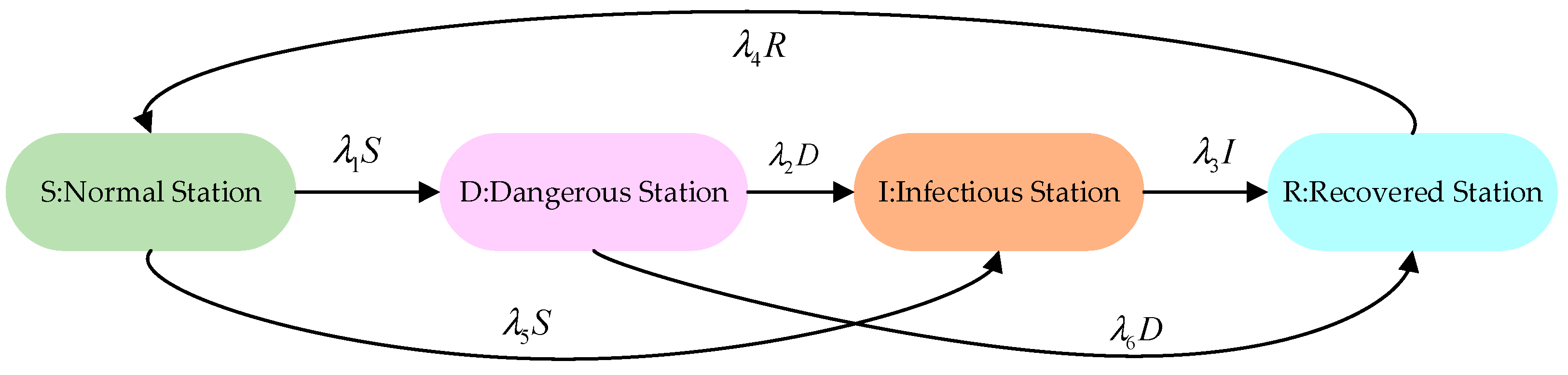
3.3.2. Propagation Mechanism

(1)

Risk backward propagation

The process of risk backward propagation at a station is the process by which station risk leads to a decline in resilience at upstream stations due to increased logistical pressure. The station’s transition from being impacted to recovery can be carefully delineated by the different risk states of the station, which can be expressed as in Figure 3.

(2)

Failure forward propagation

In the sea–rail intermodal transportation network, the process of failure forward propagation at a station is the process of cargo hoarding or transportation disruption at the downstream station due to a failure at the station. The core role of the balancing strategy is to enhance the resilience of the network by dynamically adjusting the distribution of loads, especially when the station fails, which can prevent the interruption and accumulation of cargo flow and reduce the pressure on the whole transportation network. Therefore, the hub station balancing strategy can be expressed as:

$$\Delta W_{FFC}^{i\to M_q}\left(t\right)=W_i\left(t\right)\left[\theta {\displaystyle \frac{A_{q_1}\left(t_0\right)-W_{q_1}\left(t\right)}{{\displaystyle {\sum }_{q_1\in M_q}\left(A_{q_1}\left(t_0\right)-W_{q_1}\left(t\right)\right)}}}+\vartheta {\displaystyle \frac{A_{q_2}\left(t_0\right)}{{\displaystyle {\sum }_{q_2\in M_q}{A}_{q_2}\left(t_0\right)}}}\right],\theta +\vartheta =1,$$

(4)

where $\Delta W_{FFC}^{i\to M_q}\left(t\right)$ denotes the load increment distributed from the hub station $i$ to its neighboring stations $M_q$ at the time $t$. $M_q$ denotes the functional station set of the neighboring stations $q$ of the hub station $i$, $M_q=\{q_1,q_2\}$. $\theta$ is a load redistribution parameter based on residual capacity, which indicates the extent to which the load is shifted to a station with a larger residual capacity, and $\vartheta$ is a load redistribution parameter based on the intermediary strength, which indicates the extent to which the load is shifted to a station with a stronger intermediary. Then, ${\displaystyle \frac{A_{q_1}\left(t_0\right)-W_{q_1}\left(t\right)}{{\displaystyle {\sum }_{q_1\in M_q}\left(A_{q_1}\left(t_0\right)-W_{q_1}\left(t\right)\right)}}}$ denotes the proportion of the remaining capacity of the station $q_1$ among all neighboring stations $q$ of the hub station $i$ at time $t$, and ${\displaystyle \frac{A_{q_2}\left(t_0\right)}{{\displaystyle {\sum }_{q_2\in M_q}{A}_{q_2}\left(t_0\right)}}}$ denotes the proportion of the intermediary strength of the station $q_2$ among all neighboring stations $q$ of the hub station $i$ at time $t$.

When non-hub stations have different extents of failure or risk status, the non-hub station balancing strategy redistributes its load to neighboring stations efficiently through a flexible load distribution mechanism, avoiding the collapse of the whole transportation network or the serious decline of transportation efficiency due to the failure of a single station. Therefore, the non-hub station balancing strategy is formulated based on the different failure states and risk states of non-hub stations, which can be expressed as follows:

$$\Delta W_{FFC}^{i\to j}\left(t\right)=\left\{\begin{array}{c}\left[W_i\left(t\right)-W_i\left(t_0\right)\right]{\displaystyle \frac{A_j\left(t_0\right)}{{\displaystyle {\sum }_{{j\in S}_j}{A}_j\left(t_0\right)}}},i\in M_2\cap i\in D\\ \left[W_i\left(t\right)-A_i\left(t_0\right)\right]{\displaystyle \frac{A_j\left(t_0\right)}{{\displaystyle {\sum }_{{j\in S}_j}{A}_j\left(t_0\right)}}},i\in M_2\cap \left(i\in S\cup i\in R\right)\\ W_i\left(t\right){\displaystyle \frac{A_j\left(t_0\right)}{{\displaystyle {\sum }_{{j\in S}_j}{A}_j\left(t_0\right)}}},\left(i\in M_2\cup i\in M_3\right)\cap i\in I\end{array}\right.$$

(5)

$$W_i\left(t+\Delta t\right)=\Delta W_{FFC}^{i\to j}\left(t\right)+W_i\left(t\right),$$

(6)

where $M_2$ represents the set of partial failure stations, $M_3$ represents the set of complete failure stations, and $\Delta W_{FFC}^{i\to j}\left(t\right)$ denotes the load increment distributed from the non-hub station $i$ to its neighboring stations $j$ at time $t$.

When a non-hub station $i$ is in the partial failure state $M_2$ and the risk dangerous state $D$, the load in excess of the initial load $W_i\left(t\right)-W_i\left(t_0\right)$ of the non-hub station $i$ at time $t$ is allocated to its neighboring stations $j$. This rule is designed to prevent some failure stations from failing completely due to overload, while also alleviating network pressure through load transfer. When a non-hub station $i$ is in the partial failure state $M_2$ and the risk-susceptible and recovered state $S\cup R$, the load in excess of the initial capacity $W_i\left(t\right)-A_i\left(t_0\right)$ of the non-hub station $i$ at time $t$ is allocated to its neighboring stations $j$. This rule ensures that the station can handle part of the load even when the risk is low, while avoiding over-reliance on nearby stations. When a non-hub station $i$ is in a failure $M_2\cup M_3$ and risk-infectious state $I$, the load $W_i\left(t\right)$ of the non-hub station $i$ for the moment is distributed to its neighboring stations $j$. This rule is used to handle stations that have completely failed or are at high risk, preventing cascading failures by quickly transferring the load.

(3)

Interactive propagation

For interactive propagation, the two propagation mechanisms of risk and failure work together in the network, and the propagation and evolution of risk in the network will affect the distribution of load traffic and the state of station failure. At the same time, failure also triggers new risk propagation. At time $t_0$, a station $i$ failure triggers the propagation of risk from a station in the network. At the $t_0+\Delta t$ moment, the risk propagates backward to the $n_{BRP}$ layer. At the same time, the failure propagates forward to the $m_{FFC}$ layer. The process can be expressed as Equations (7) and (8):

$${\tau }_{BRP}={\displaystyle \frac{n_{BRP}}{\left(t_0+\Delta t\right)-t_0}},$$

(7)

$${\tau }_{FFC}={\displaystyle \frac{m_{FFC}}{\left(t_0+\Delta t\right)-t_0}},$$

(8)

where ${\tau }_{BRP}$ represents the risk propagation rate and ${\tau }_{FFC}$ represents the failure propagation rate.

Introducing the propagation interaction coefficient $\zeta$, the extent of the risk–failure interactive propagation can be expressed as:

$$\zeta ={\displaystyle \frac{{\tau }_{BRP}}{{\tau }_{FFC}}}={\displaystyle \raisebox{1ex}{$\frac{n_{BRP}}{\left(t_0+\Delta t\right)-t_0}$}\!\left/ \!\raisebox{-1ex}{$\frac{m_{FFC}}{\left(t_0+\Delta t\right)-t_0}$}\right.}={\displaystyle \frac{n_{BRP}}{m_{FFC}}},$$

(9)

where, when $\zeta >1$ and $\zeta$ is larger, it means that the risk propagates faster in the network compared to the failure propagation per elapsed time $\Delta t$.

The complexity of the risk state of the stations in the network leads to a certain extent of randomness in the risk triggered by the failure state stations. In this paper, the quantile distribution of the cumulative distribution function of the standard normal distribution was used as a probabilistic model of the risk occurrence process of the partial failure station to reflect the stochastic process of the failure-induced risk. Its basic form is:

$${\rm P}\left(E_i=D\left|Y_i\in \left(0,1\right)\right.\right)=\mathrm{\Phi }\left({\mathrm{{\rm Z}}}_i\right),{\mho }_i\in \left(0,1\right),$$

(10)

$${\mho }_i={\displaystyle \frac{d_i^{out}}{d_i^{in}+d_i^{out}}},$$

(11)

$$\mathrm{\Phi }\left({\mathrm{{\rm Z}}}_i\right)={\displaystyle \frac{{\displaystyle {\int }_{-\infty }^{{\mathrm{{\rm Z}}}_i\left(t\right)}}\exp \left(-\frac{1}{2}{t}^2\right)dt}{{\displaystyle {\int }_{-\infty }^1}\exp \left(-\frac{1}{2}{t}^2\right)dt}},{\mathrm{{\rm Z}}}_i={\xi }_1{\mho }_i{Y}_i+{\xi }_2{\mho }_i\zeta +{\xi }_3{\mho }_i,$$

(12)

where ${\rm P}\left(E_i=D\left|Y_i\in \left(0,1\right)\right.\right)$ is the probability of a partial failure station $i$ triggering a risk at time $t$, $d_i^{in}$ represents the in-degree value of a station $i$ in the network, and ${\mho }_i$ represents the out-degree value of a station in the network and is the out-degree scale factor. The larger the ${\mho }_i$ value, the larger the proportion of the downstream stations of the representative station to all neighboring stations. ${\xi }_1$, ${\xi }_2$, and ${\xi }_3$ are the determined parameters, and ${\mathrm{{\rm Z}}}_i$ represents the functional relationship between the station failure state function $Y_i$, the out-degree scale factor ${\mho }_i$, and the propagation interaction coefficient $\zeta$.

3.3.3. Repair Mechanism

The repair mechanism primarily consists of transportation route fine-tuning during restoration and restoration termination. These two components are described as follows:

(i)

Transportation route fine-tuning during restoration

When station interruptions occur, affected stations require a certain period for restoration. During this period, as the transportation network encompasses railway and liner transportation modes, the route adjustment patterns and characteristics differ. Considering the distinctions between railway and liner transportation in route adjustments, the model selects target stations for skip–stop operations along the affected service routes. This approach effectively adjusts transportation routes to ensure the continuity and efficiency of freight transportation while minimizing the impact of station failure to the greatest extent possible.

When selecting target alternative stations for skip–stop operations, it is essential to comprehensively consider factors such as the cargo’s destination country and voyage time. Priority is typically given to neighboring stations within the same region as the disrupted station. Based on these considerations, we define a set of alternative stations $s^{\prime }$ for each station $s$ along every transportation route, which must satisfy the following requirements:

(a) The target station $s^{\prime }$ must be a downstream station $s_j$ of the disrupted station $s$, i.e., $s^{\prime }\in \left\{s_j\right\}$, where $j$ denotes the index of stations located downstream of $s$ along the transportation route. Specifically, if the disrupted station is at position $i$, the set of downstream stations $\left\{s_j\right\}$ includes all stations satisfying $j\ne i$ within the same route and region.

(b) For liner station transportation routes, the distance between the target liner station $s^{\prime }$ and the disrupted station should be maintained within a reasonable proximity to avoid long-distance detours during transportation. Specifically, the distance between the target station $s^{\prime }$ and the disrupted station’s upstream station $s_k$ must not exceed the average segment length of the original shipping route. This constraint can be expressed as:

$$d\left(s_k,s^{\prime }\right)\le {\displaystyle \frac{1}{n}}{\displaystyle \sum _{n=1}^{n}d(s,s_j)},$$

(13)

where $d(s_k,s^{\prime })$ denotes the distance between the target station $s^{\prime }$ and the upstream station $s_k$ of the disrupted station, $d(s,s_j)$ represents the distance between the disrupted station $s^{\prime }$ and its downstream station $s_j$, $S_0,S_1,\dots ,S_n\in \left\{s_j\right\}$; $S_0,S_1,\dots ,S_n$ constitute the sequence of downstream stations of the disrupted station in the original transportation route, and $n$ is the total number of distance segments.

For railway station transportation routes, the transportation routes operate round-trip along predefined station sequences. Therefore, when a station failure occurs, the system bypasses the disrupted railway station. The distance between the upstream station $s_k$ of the disrupted station and the target station $s^{\prime }$ equals the sum of the distance from the upstream station $s_k$ to the disrupted station $s$ and the distance from the disrupted station $s$ to its downstream station $s_j$. This can be expressed as:

$$d\left(s_k,s^{\prime }\right)=d\left(s_k,s\right)+\dots +d\left(s,s^{\prime }\right),$$

(14)

where $d(s,s^{\prime })$ denotes the distance between the disrupted station $s$ and its downstream station $s_j$.

For hub transportation routes, the repair mechanism is divided into three scenarios:

If both the upstream station and downstream station are liner stations, apply Equation (13).

If both the upstream station and downstream station are railway stations, apply Equation (14).

If the upstream and downstream stations are of different operational types (e.g., one liner and one railway station), the route will remain interrupted during restoration without selecting alternative stations.

(c) Target stations must maintain functionality. In practical operations, the transportation route will randomly select a target station from the predefined set of alternative stations. If the selected target station subsequently becomes disrupted, the route can select another station from the alternative set again; if no functional target stations are available, the route will be interrupted and undergo restoration.

Based on the above rules, the given transportation route is treated as input data. The transportation network is modeled as a bipartite network $G=(R,V,E)$, where $R$ and $V$ represent the sets of transportation routes and stations, respectively. $E$ denotes the edge set between $R$ and $V$, such that an edge exists in $E$ between a transportation route and a station if the station is included in that route. The station network $G^{\prime }=(V,E^{\prime })$ is derived from the single-mode projection of $G$. Here, $E^{\prime }$ represents the set of inter-station edges, where a directed edge exists between two stations if they are co-located in at least one transportation route. The process of adjusting transportation routes for a specific disrupted station during restoration is illustrated in Figure 4.

(ii)

Restoration termination

A failure station is temporarily shut down for a time step $T$, while the propagation of risk–failure caused by it continues. The station recovery time depends on the station functionality and speed of recovery, and can be expressed as the following equation:

$$T={\displaystyle \frac{A_i\left(t_0\right)}{\gamma }},$$

(15)

where $C_i\left(t_0\right)$ represents the capacity of the station $i$, which is used as a measure of the state of the station when it is functioning normally, and $\gamma$ denotes the speed of restoration.

In the repair mechanism, when two neighboring stations are both in a risk recovered state, the network restores the transportation routes of its upstream or downstream stations so that the stations are able to regain new loads. The repair process ends when the risk status of all stations in the network no longer changes. In this case, there is a certain probability of repairing the failure transportation routes between stations with risk recovered status, and the probability formula is expressed as:

$$SIM\left(p,k\right)={\displaystyle \frac{\left|{\Gamma }_p\left(t\right)\cup {\Gamma }_k\left(t\right)\right|}{\max \left\{\left|{\Gamma }_p\left(t_0\right)\right|,\left|{\Gamma }_k\left(t_0\right)\right|\right\}}},p,k\in R_i,$$

(16)

where $SIM\left(p,k\right)$ represents the likelihood of transportation route restoration between two stations via a third-party station, ${\Gamma }_p\left(t\right)$ and ${\Gamma }_k\left(t\right)$ are, respectively, the set of neighboring stations for the risk recovered status station $p$ and station $k$, $\left|{\Gamma }_p\left(t\right)\cup {\Gamma }_k\left(t\right)\right|$ represents the set of neighboring stations for the station $p$ and the station $k$ at time $t$, and $\max \left\{\left|{\Gamma }_p\left(t_0\right)\right|,\left|{\Gamma }_k\left(t_0\right)\right|\right\}$ represents the set of neighboring stations for the station $j$ and the station $k$ at time $t_0$.

3.4. Resilience Metric

In order to better quantify the improvement of the resilience of the Belt and Road transportation network by the recovery strategy, this paper adopted the network failure rate $\mu \left(t\right)$, the network maximum connectivity rate $\Psi \left(t\right)$, and the network efficiency $E(t)$ based on the station failure extent to evaluate the network resilience. They can be expressed as follows:

$$\mu \left(t\right)={\displaystyle \frac{1}{M}}\left\{{\displaystyle \sum _{i\in M_3}{x}_i}+{\displaystyle \sum _{i\in M_2}\left[1-\frac{W_i\left(t_0\right)-A_i\left(t_0\right)}{{\theta }_i\left(t\right)A_i\left(t_0\right)-A_i\left(t_0\right)}\right]}{\epsilon }_i\left(t\right)\right\},$$

(17)

$$\Psi \left(t\right)={\displaystyle \frac{{\displaystyle \sum _{i\in M_1}{d}_i^1\left(t\right)}+{\displaystyle \sum _{i\in M_2}{d}_i^2\left(t\right)}+{\displaystyle \sum _{i\in M_3}{d}_i^3\left(t\right)}}{{\displaystyle \sum _{i\in M}{d}_i\left(t_0\right)}}},$$

(18)

$$E(t)={\displaystyle \frac{1}{N(N-1)}}{\displaystyle \sum _{i\ne j\in M}\frac{1}{d_{ij}(t)}},$$

(19)

where ${\displaystyle \sum _{i\in M_1}{d}_i^1\left(t\right)}$ represents the set of normal state station degree at the time $t$, ${\displaystyle \sum _{i\in M_2}{d}_i^2\left(t\right)}$ represents the set of partial failure station degree at the time $t$, ${\displaystyle \sum _{i\in M_3}{d}_i^3\left(t\right)}$ represents the set of complete failure station degree at the time $t$, and ${\displaystyle \sum _{i\in M}{d}_i\left(t_0\right)}$ is the set of station metrics at the initial moment $t_0$. $M_1$ represents the set of normal state stations in the network, $M$ represents the set of all stations in the network, i.e., $M_1\cup M_2\cup M_3=M$, $N$ represents the number of stations in the network, $d_{ij}(t)$ represents the shortest path distance between station pairs $\left(i,j\right)$, and ${\displaystyle \frac{1}{d_{ij}(t)}}$ represents the efficiency of station pairs $\left(i,j\right)$.

4. Simulation Validation

To verify the effectiveness of the proposed model, extensive simulation experiments were implemented on an Intel Core i5-12500H 2.5 GHz PC with 16 G memory and performed in MATLAB R2022a.

4.1. Transportation Network Design

The sea–rail intermodal transportation involves two modes of transport, namely, liner transport and railway transport. The transportation network followed a core-periphery hierarchical structure, forming a coexistence structure of hub and single-mode transportation stations. The sea–rail intermodal transportation network model in this paper was based on the transportation route data released by the Belt and Road Initiative. The Belt and Road transportation network consists of 197 stations and 1999 transportation routes [47,48]. The specific topology of the network plotted using ArcGIS 10.8 is shown as follows.

As shown in Figure 5, the stations connected by yellow transportation routes represent the Land Silk Road transportation network, while the stations connected by blue transportation routes represent the Maritime Silk Road transportation network. The two transportation networks are connected through hub stations located along the coasts and identified by red five-pointed stars. The key stations of the Land Silk Road and the Maritime Silk Road are not only limited to these hub stations. The transportation routes also converge at the liner and railway stations, realizing a closer interconnection of transportation networks.

4.2. Validation of Model Effectiveness

To examine the validation of the network risk–failure interactive propagation and recovery model effectiveness, this paper analyzed the network resilience under hybrid- and single-attack modes and compared resilience recovery. The hybrid attack model proposed in this paper includes three single-mode attacks: (1) degree attack is the node with the highest degree of priority attack, (2) betweenness attack is the priority attack on the node with the strongest intermediation in the network, and (3) closeness attack is the priority attack on the node with the highest proximity to centrality in the network. The simulation parameters were set as follows: ${\beta }_i=0.4$, ${\theta }_i\left(t\right)=2$, ${\lambda }_1=0.2$, ${\lambda }_2=0.5$, ${\lambda }_4=0.5$, and ${\lambda }_5=0.8$.

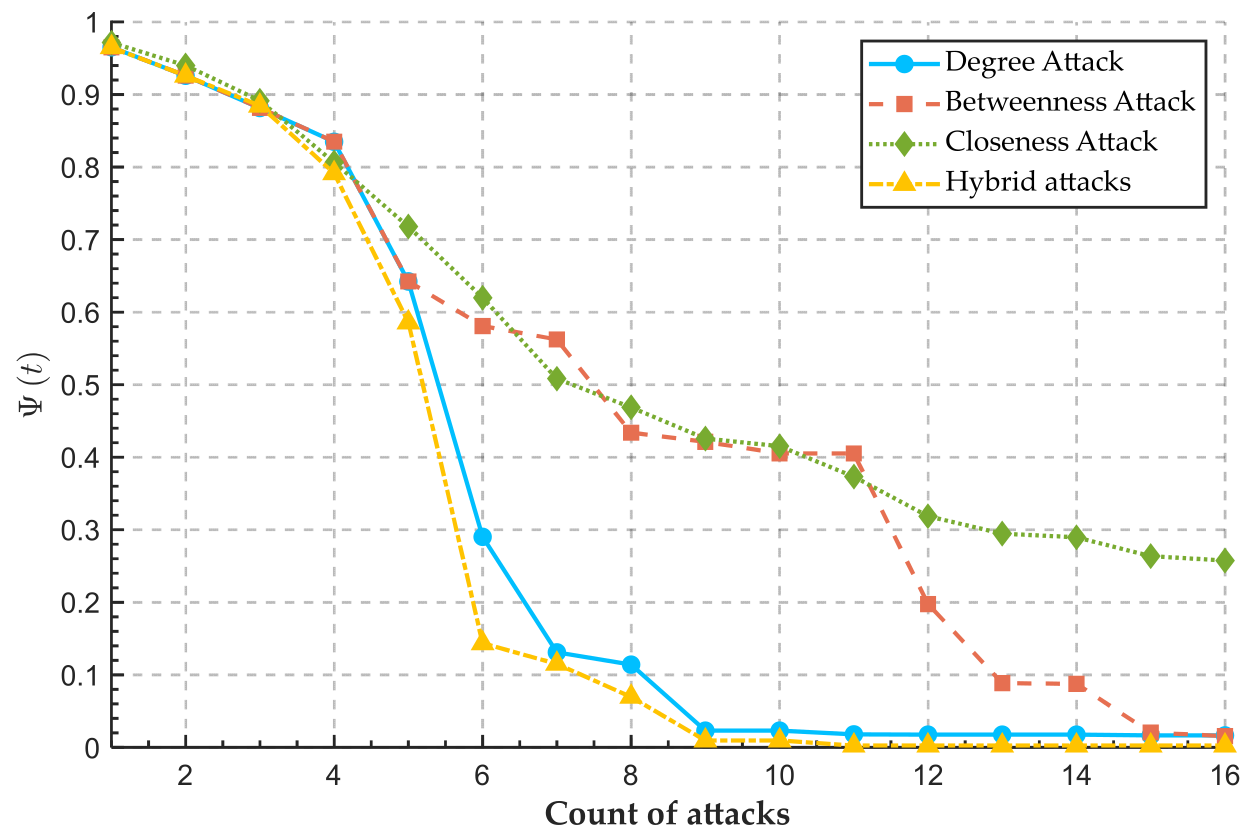
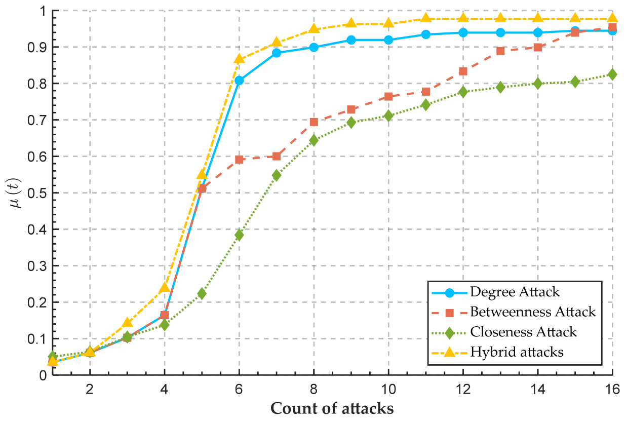
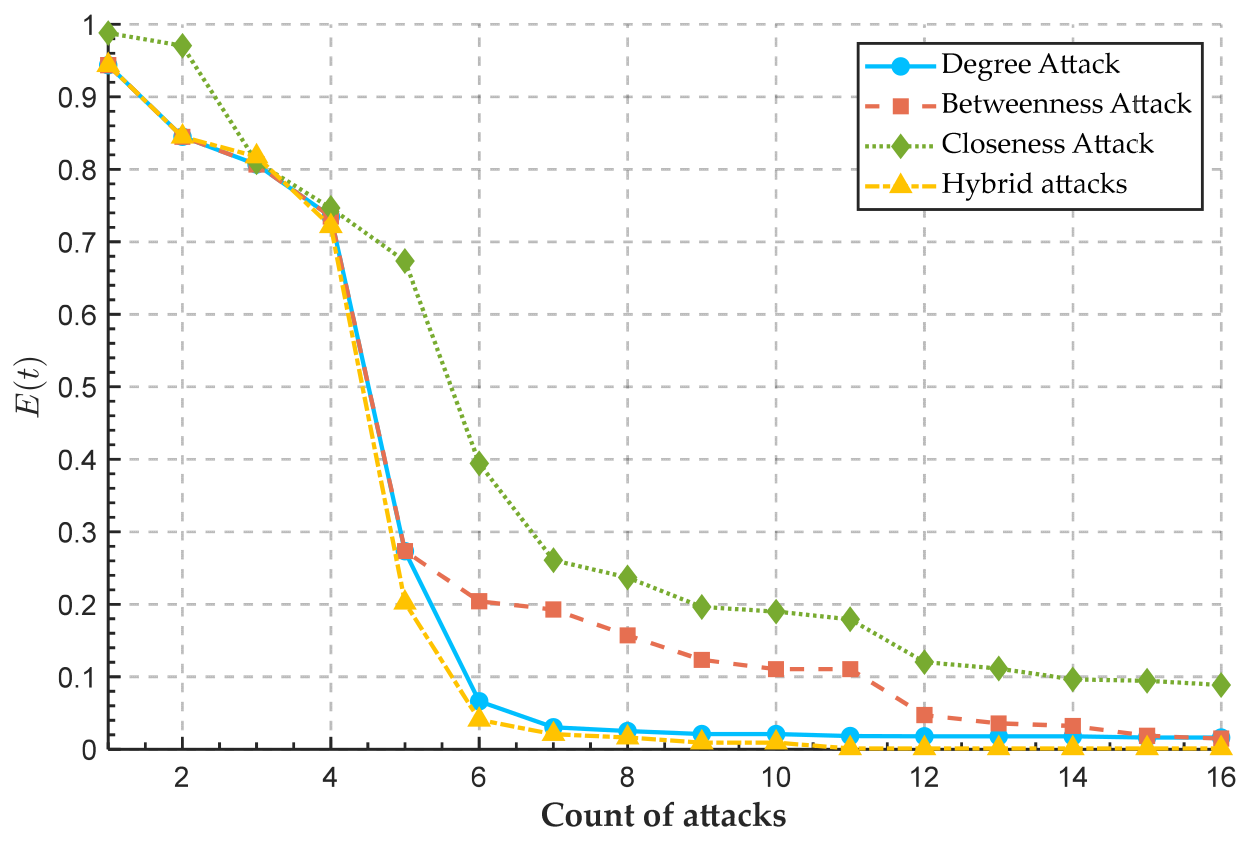
4.2.1. Different Attack Modes

We explored the impact of the sea–rail intermodal transportation network among the degree, betweenness, closeness, and the proposed hybrid attack mode. The simulation results are shown in Figure 6, Figure 7 and Figure 8.

As depicted in Figure 6, when the 4th station attack occurred, the hybrid attack caused a cliff-like decline of $\Psi \left(t\right)$. The extent of decline was more severe than any single-attack mode. By the 6th attack, $\Psi \left(t\right)$ dropped below 20% under the hybrid attack mode, while the performance of the remaining attack modes remained above 25%. However, compared with Figure 7 and Figure 8, under the ending closeness attack, the decline of $\mu \left(t\right)$ and $E(t)$ was the slowest among the other three attacks. Moreover, in the first six attacks, the extent of decline of the hybrid and degree attacks was similar, both significantly reducing in the middle period of attacks, that is, during the 4th to 6th attacks. Based on the simulation results in Figure 6, Figure 7 and Figure 8, there were significant differences between hybrid attack and single-attack modes in terms of network destruction mechanisms and performance response.

Hybrid attacks exhibit unparalleled destructiveness in the sea–rail intermodal transportation network due to their multifaceted targeting attack strategy, which synergistically exploits degree, betweenness, and closeness centrality. Unlike single-metric attacks, hybrid modes induce nonlinear performance collapse by eliminating stations that bridge connectivity, routing, and dynamic coordination. This mechanistic superiority underscores the necessity of incorporating hybrid attack scenarios into network vulnerability assessments, particularly for critical infrastructure with multifunctional stations.

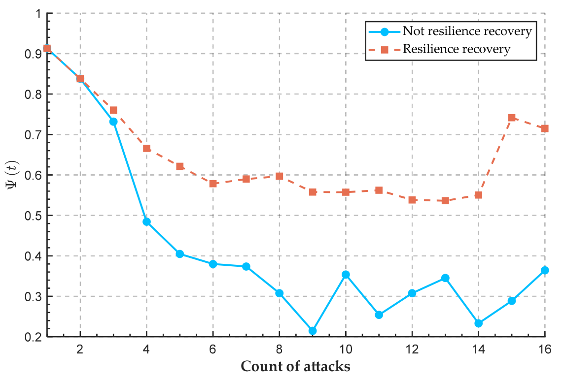
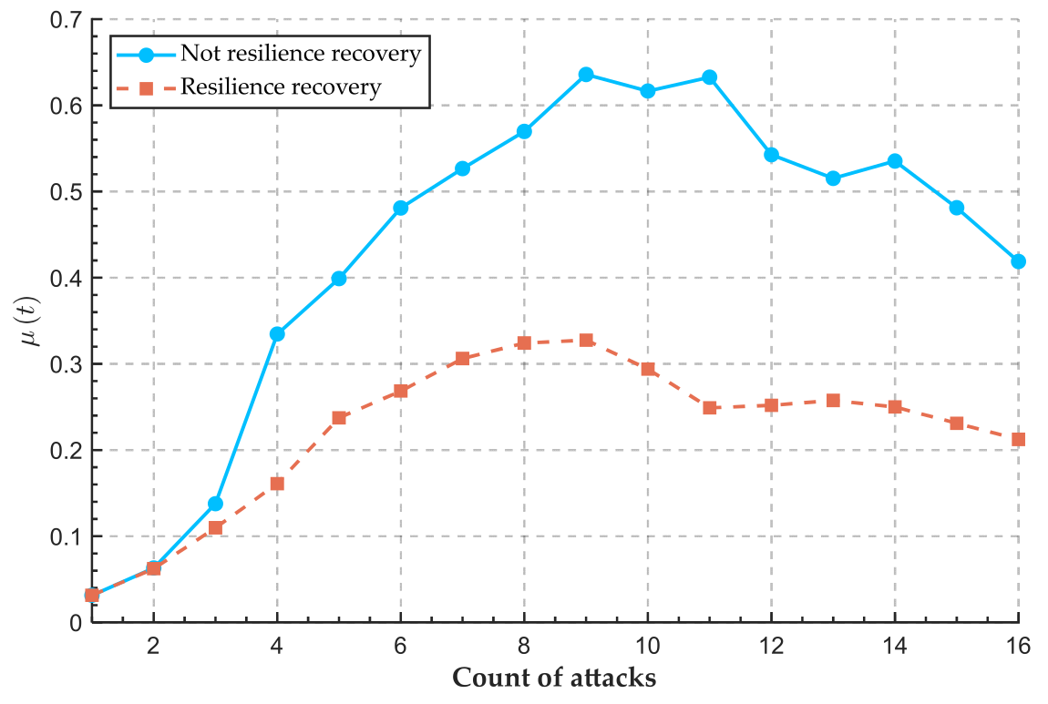
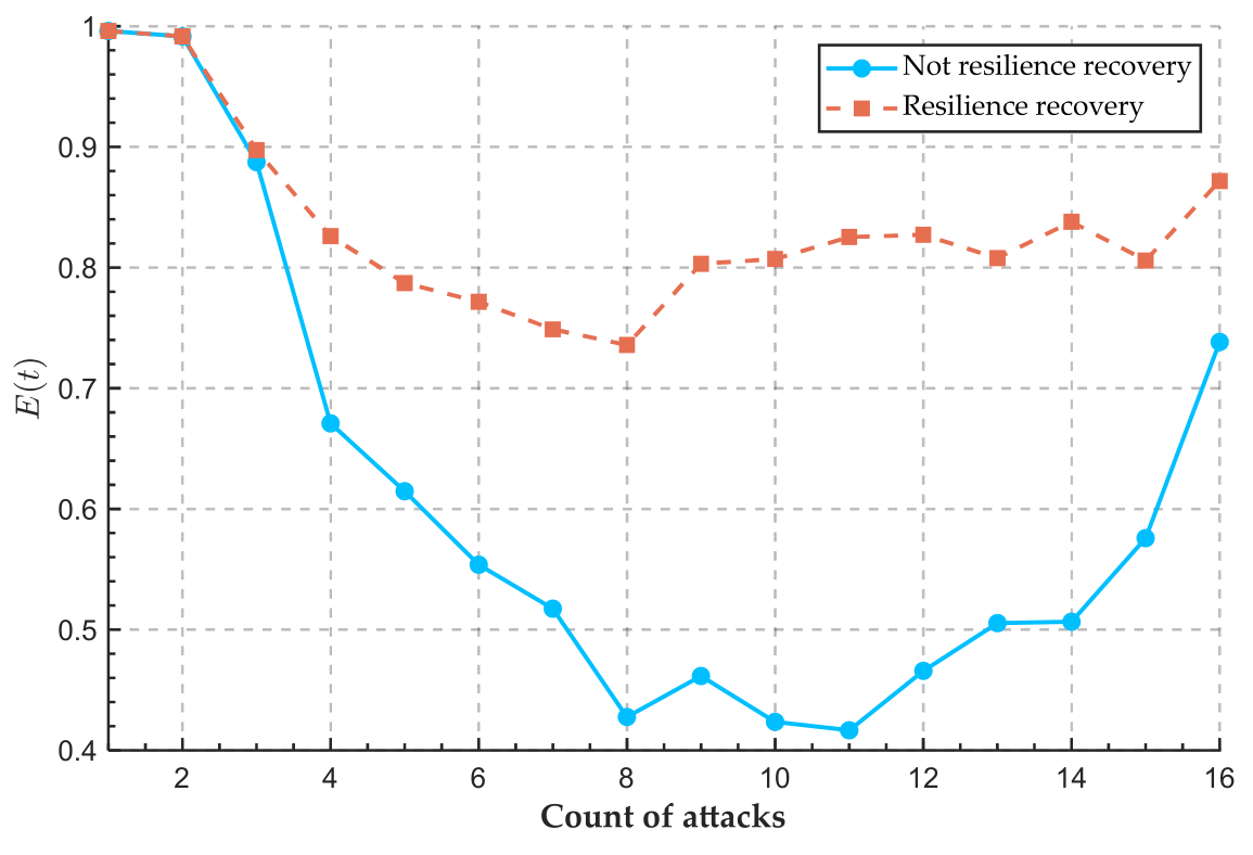
4.2.2. Resilience Recovery

We explored the impact of whether or not the sea–rail intermodal transportation network carried out a resilience recovery mechanism on the network resilience under the hybrid attack mode. The simulation results are shown in Figure 9, Figure 10 and Figure 11.

As shown in Figure 9, Figure 10 and Figure 11, it can be seen that the sea–rail intermodal transportation network with resilience recovery was more moderate in terms of resilience degradation compared to the network without resilience recovery in the same period of time. The resilience recovery mechanism ensured that throughout the entire attack period, the network $\Psi \left(t\right)$ remained no lower than 0.5 and $\mu \left(t\right)$ remained no higher than 0.4, and the network $E(t)$ remained no lower than 0.7. In contrast, $\Psi \left(t\right)$ of the non-resilience recovery mechanism started to perform lower than 0.4, $\mu \left(t\right)$ performed higher than 0.4, and $E(t)$ performed lower than 0.6 from the 5th attack. Moreover, the ordinary recovery mechanism caused significant fluctuations in network performance, especially with the difference between its minimum and maximum values beyond twice that of the resilience recovery mechanism. In scenarios lacking resilience recovery mechanisms, the hybrid attack induced a rapid collapse of network functionality.

Multidimensional metrics showed that the implementation of the resilience recovery mechanism not only mitigated the decline in network resilience but also shortened the time required for the network to fully recover from disruption, which significantly enhanced the resilience of the sea–rail intermodal transportation network in actual operation. The absence of resilience recovery mechanisms exacerbated the impacts of hybrid attack, leading to irreversible network fragmentation. Proactive recovery strategies, particularly those prioritizing the restoration of critical stations and adaptive routing, are crucial for maintaining operational continuity in multimodal transportation systems under adversarial conditions.

5. Case Study

Concerning how to make the resilience recovery of networks efficient in practice, the following three aspects will be investigated: Section 5.1 focuses on repair capacity adjustment, Section 5.2 discusses the risk management, and Section 5.3 explores the hub station allocation equalization.

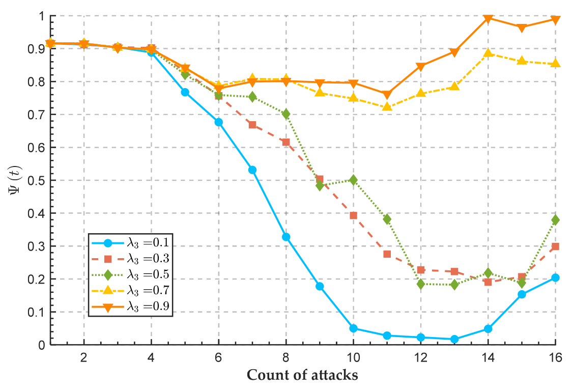
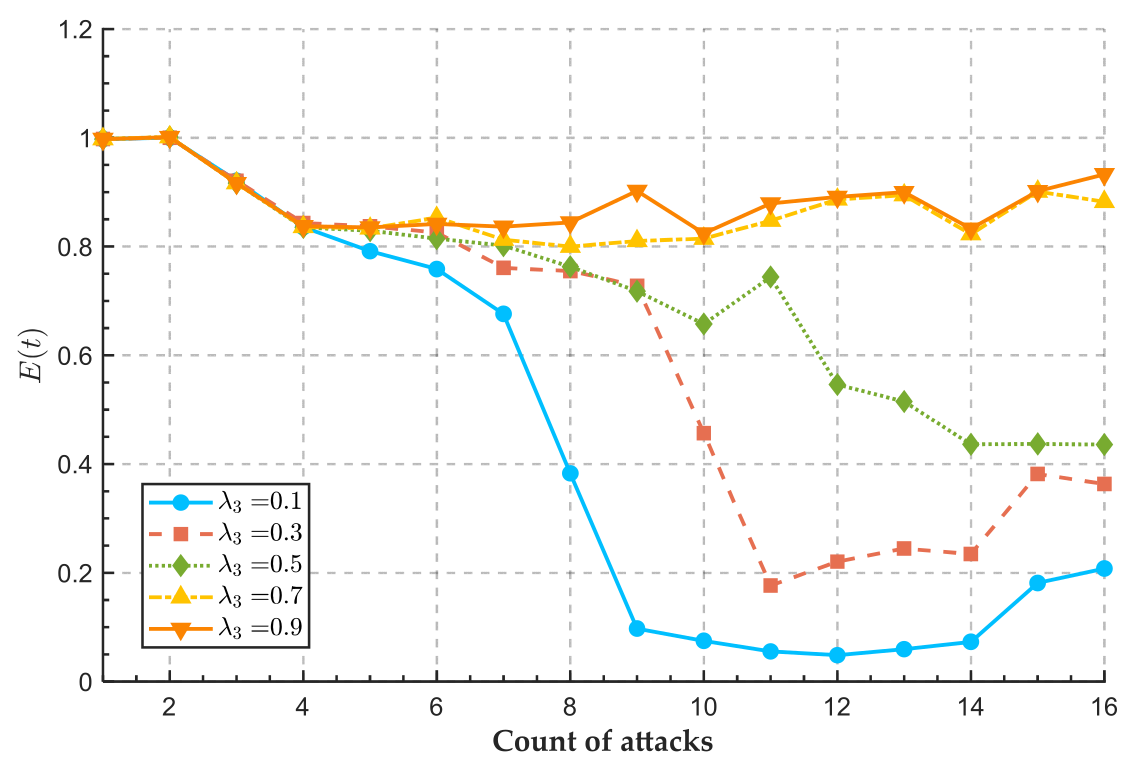
5.1. Repair Capacity Adjustment

The Red Sea crisis in January 2024 led to partial closures and route cancellations at ports, including Eilat Port and King Abdullah Port. Due to prolonged restoration periods at affected ports, a significant number of vessels were forced to reroute around the Cape of Good Hope, making South Africa’s Durban Port one of the most severely congested hubs, with cascading impacts on global transportation networks. This chain reaction highlighted port restoration capability as a critical factor in transportation network resilience, where repair timelines directly determine the recovery efficiency of entire logistics systems.

As a key factor in controlling network recovery, adjusting the repair capacity directly affects the length of the repair time. Here, we explored the sea–rail intermodal transportation network resilience changes under the station repair time $T\in \left(5, 10\right]$, in which the station repair time is mainly used to control the time required to repair the failure station to the normal state. The simulation results are shown in Figure 12, Figure 13 and Figure 14.

The simulation results in Figure 12, Figure 13 and Figure 14 systematically evaluate the relationship between station repair time and the resilience recovery dynamics of sea–rail intermodal transportation networks under the hybrid attack scenario. As shown in Figure 12 and Figure 13, the shortening of the station repair time weakened the interdependence between stations, and the minimum of $\Psi \left(t\right)$ and $\mu \left(t\right)$ gradually increased. As shown in Figure 14, when $T=6~8$, the evolution trend of $E(t)$ was similar. It can be seen that when the repair time was shortened, the increase in the station repair time made the minimum of $E(t)$ show a more obvious decreasing trend, and the corresponding network failure rate peaked into a rising trend.

Considering the above three metrics, the prolongation of the failure station repair time in the network led to the expansion of the failure area and the increase of the complexity of the network resilience recovery process. If a station failed to be restored within a short period of time, its route may trigger new failure, which would lead to a decrease in the efficiency of the failure station, a decrease in the network connectivity, and an increase in the failure rate of the corresponding station. Therefore, reducing the station repair time enhances network resilience by decoupling station interdependencies and curbing failure propagation. However, this requires strategic resource allocation to mitigate transient efficiency losses. The optimal repair time, $T=6~7$, balances rapid recovery with system-wide stability, providing actionable insights for designing adaptive repair protocols in multimodal transportation networks.

5.2. Risk Management

The risk recovery rate ${\lambda }_3$ serves as a key indicator for measuring port resilience, reflecting a port’s capability to restore normal operations from risk-exposed conditions. This metric demonstrates a positive correlation with a port’s risk management capacity. The stronger the management capability, the higher the risk recovery rate. Taking Phase 1 of Singapore’s Tuas Port as an example, the implementation of an AI-driven intelligent monitoring system has enabled real-time dynamic management of terminal safety and traffic coordination, significantly enhancing risk response efficiency. This AI-powered risk management advancement not only ensures operational stability at Tuas Port but also substantially strengthens the systemic resilience of the entire transportation network. Simulation analysis examining the impact of varying risk recovery rates, ${\lambda }_3\in \left[0.1, 1.0\right)$, on network resilience is presented in Figure 15, Figure 16 and Figure 17.

As ${\lambda }_3$ increased from 0.1 to 0.9 and recovering stations reintegrated into the network, $\Psi \left(t\right)$ improved by 73% in Figure 15 and restored critical linkages between maritime and railway. As can be seen in Figure 16, the global network failure rate $\mu \left(t\right)$ reduced by 81%. This decline was attributed to accelerated recovery of compromised stations, which limited failure propagation through rapid resource reallocation. In addition, $E(t)$ increased by 88% in Figure 17, driven by reduced path redundancy and optimized cargo flow redistribution. Therefore, high ${\lambda }_3$ enabled faster clearance of cargo backlogs at critical stations, lowering network-wide congestion, and ${\lambda }_3=0.9$ was the optimal risk recovery rate.

Higher station risk state recovery rates ${\lambda }_3$ mean that the network is able to return to normal from a risk-infectious state more quickly, which reduces the overall duration of network risk and reduces the likelihood of failure propagation through the network. The faster a station recovers, the more quickly it can handle backlogs, reduce network load, and restore connectivity to other stations, which in turn improves overall connectivity and efficiency. Increased network connectivity allows goods and information to flow more smoothly and reduces the global impact of individual station failure, thereby increasing the overall resilience and recovery of the network.

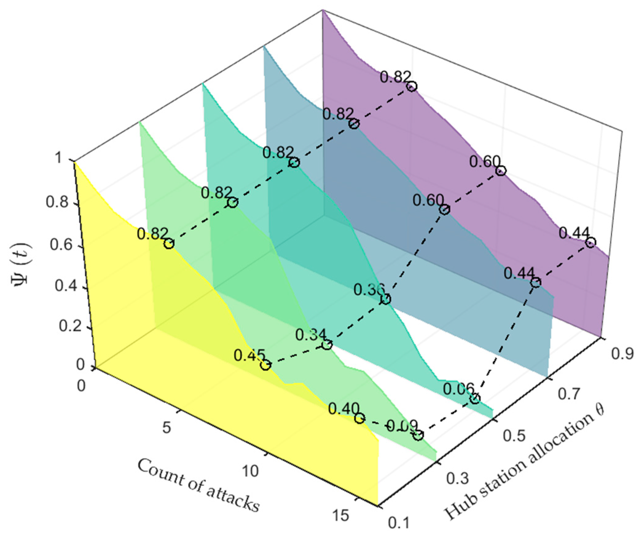
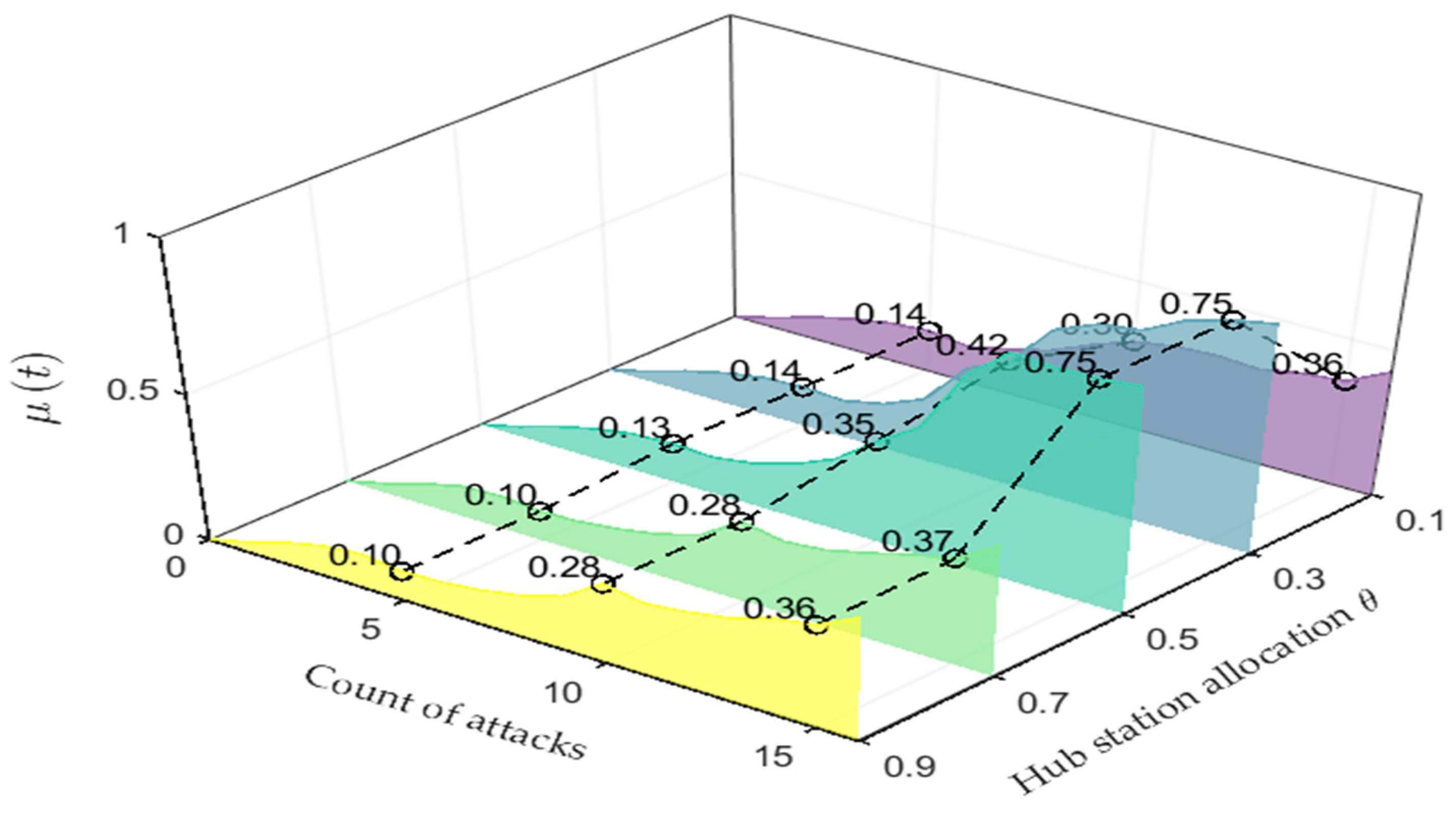
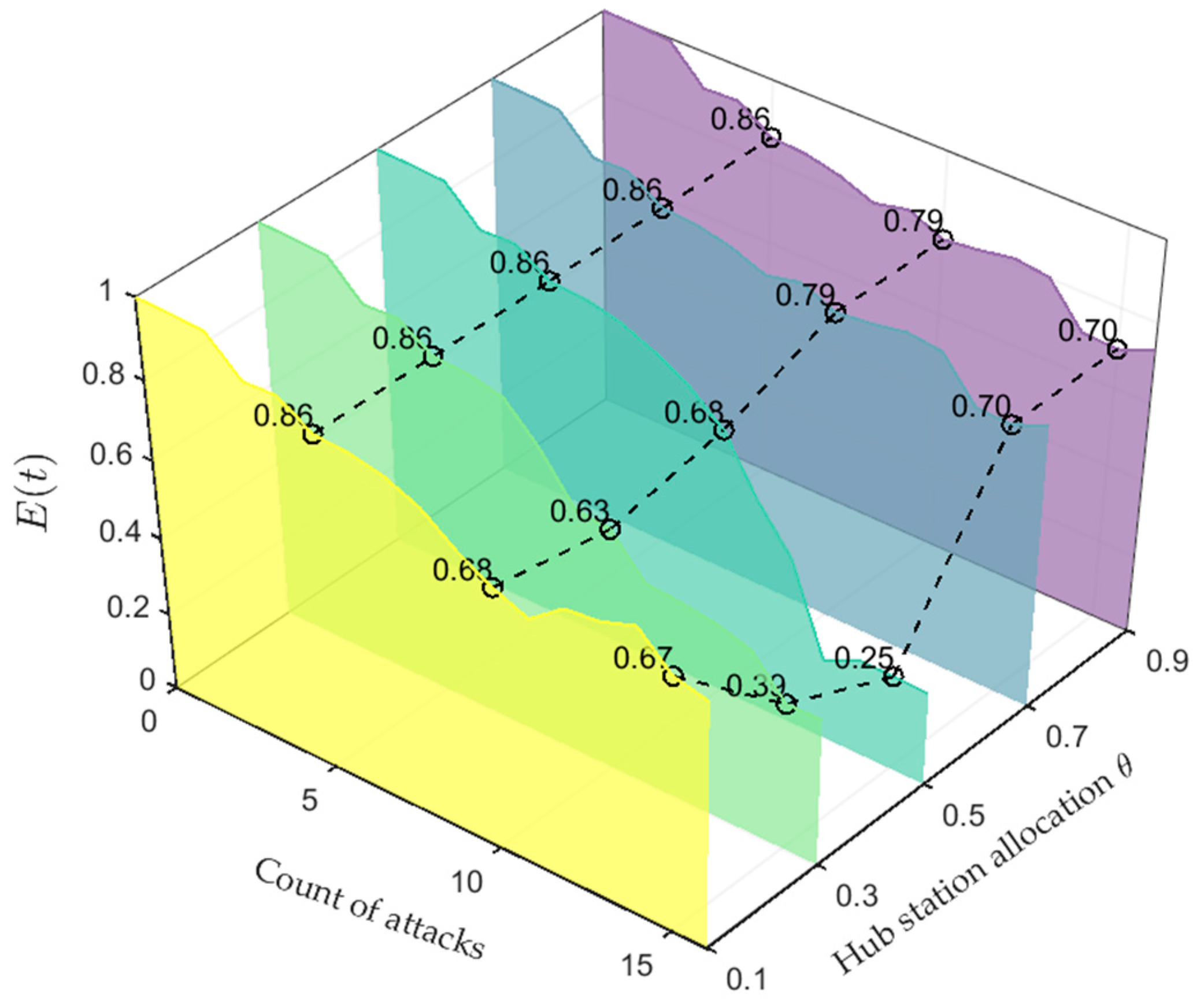
5.3. Hub Station Allocation Equalization

The Red Sea crisis in January 2024 led to the closure of affected ports, forcing shipping companies to dynamically reroute cargo to alternative ports or adjust shipping lanes (e.g., many opted to reroute around the Cape of Good Hope in Africa instead of the Red Sea). This resulted in severe congestion at other ports, such as the Port of Durban, due to sudden route adjustments, causing a decline in global shipping network efficiency and a surge in freight costs. Implementing efficient dynamic cargo allocation, strengthening regional collaboration, and enhancing policy guidance can help build a more resilient and cost-controllable global shipping network. The effectiveness of distributional balancing at hub stations highly relies on the capacity ratio threshold settings. Examining how sea–rail intermodal transportation network resilience is affected by the proportion of residual or total capacity in the load-balancing strategy at the hub station determines the different load allocation rules denoted by the parameters $\theta$. To investigate the network resilience of the balancing strategy adjustment, the simulation results are shown in Figure 18, Figure 19 and Figure 20, where the range of $\theta$ is from 0.1 to 0.9, with an incremental step of 0.2.

Combining Figure 18, Figure 19 and Figure 20, the simulation results indicated that under the balanced configuration strategy $\theta =0.5$, network connectivity $\Psi \left(t\right)$ and efficiency $E(t)$ decreased by 38% and 45%, respectively, while the failure rate $\mu \left(t\right)$ increased to 34%. Compared to a balancing strategy that prioritizes total capacity, when the load distribution strategy shifted toward residual capacity $\theta =0.9$, the network connectivity $\Psi \left(t\right)$ and efficiency $E(t)$ improved by 15% and 11%, respectively, at an attack count of 10, but the failure rate $\mu \left(t\right)$ also increased by 2%. This phenomenon indicated that although the balanced configuration attempted to achieve global optimization by balancing the weights of residual capacity and total capacity, it failed to adequately differentiate the distinct resource endowments of high-capacity stations. As a result, the potential processing capacity of critical stations was not effectively released, while low-capacity stations experienced resource waste due to redundant load distribution, leading to a collapse in efficiency.

Further analysis revealed that the homogeneous load distribution of the balanced strategy exacerbated the average load pressure on stations, significantly advancing the trigger threshold for cascading failure. Moreover, due to the lack of a dynamic response mechanism for real-time load fluctuations, this strategy cannot quickly migrate traffic from overloaded stations to low-load stations, further amplifying the cumulative failure effect. It is worth noting that although the strategy prioritizing residual capacity temporarily improved efficiency by concentrating on high-capacity stations, its over-reliance on a few critical stations weakened path diversity. Once these stations fail, the insufficient backup paths will trigger a more severe global efficiency collapse. Therefore, the optimization of balanced configuration must seek a balance between short-term efficiency improvement and long-term stability, avoiding the risk of overloading critical stations through dynamic weight adjustment, and enhancing the path redundancy design to suppress failure propagation. This finding provides a theoretical basis and practical implications for the load distribution strategy optimization of the sea–rail intermodal transportation network.

6. Conclusions

In the context of global supply chains that are highly interdependent on intermodal transportation networks, the frequent occurrence of station congestion, extreme weather events, and geopolitical conflicts in recent years has shown that the failure of a single transportation station may trigger a chain reaction through the network. Traditional research focuses on the propagation analysis of a single risk or failure, which makes it difficult to effectively deal with the chain reaction and recovery delay triggered by the risk–failure interaction. This paper addressed this challenge and constructed a network risk–failure interactive propagation and recovery model, taking the sea–rail intermodal transportation network as the research object, which systematically revealed the resilience evolution regulation of the complex transportation system.

This paper broke through the limitations of the traditional single-path propagation model and realized the quantitative characterization of the dynamic coupling process of risk and failure by establishing a bidirectional interaction mechanism of failure forward and risk backward propagation between stations. Secondly, we proposed a load-balancing strategy and a restoration mechanism based on the segmentation of the extent of station failure, which, combined with multidimensional resilience assessment indexes, significantly improved the timeliness and precision of the network restoration strategy. Finally, the empirical study of the Belt and Road transportation network verified the applicability of the model in real, complex scenarios.

This study has made significant progress in the theoretical construction and empirical application of the interaction and propagation mechanism of network risk and failure but still has limitations. Firstly, the existing models were based on the topological characteristics of the sea–rail combined transport network for modeling, and although the effectiveness of the basic framework has been verified through empirical analysis of the Belt and Road transportation network, the adaptability of the model in multimodal transport networks, such as sea–land–air, has not been systematically verified. Secondly, the adjustment of current model parameters still depends on historical data, lacking a fusion mechanism for real-time dynamic data. Based on the above limitations, future research can further explore the following directions: First, expanding the interaction propagation model to a wider range of transportation network types, such as sea–air–land intermodal transportation and cross-border logistics. Second, optimizing the adaptive adjustment ability of the model parameters by combining with real-time dynamic data (e.g., meteorological disaster warnings and station congestion monitoring). Third, exploring the collaborative risk–failure prediction and restoration decision-making framework driven by artificial intelligence, so that the intelligence level of the resilience management of the complex network can be further improved.

References

1. Liu, T.; Wang, H. Evaluating the Service Capacity of Port-Centric Intermodal Transshipment Hub. J. Mar. Sci. Eng. 2023, 11, 1403. [Google Scholar] [CrossRef]
2. Macedo, F.C.; Alminhana, F.; Miguel, L.F.F.; Beck, A.T. Performance-Based Reliability Assessment of Transmission Lines under Tornado Actions. Reliab. Eng. Syst. Saf. 2024, 252, 110475. [Google Scholar] [CrossRef]
3. Li, S.; Wu, J.; Jiang, Y.; Yang, X. Impacts of the Sea-Rail Intermodal Transport Policy on Carbon Emission Reduction: The China Case Study. Transp. Policy 2024, 158, 211–223. [Google Scholar] [CrossRef]
4. Derpich, I.; Duran, C.; Carrasco, R.; Moreno, F.; Fernandez-Campusano, C.; Espinosa-Leal, L. Pursuing Optimization Using Multimodal Transportation System: A Strategic Approach to Minimizing Costs and CO2 Emissions. J. Mar. Sci. Eng. 2024, 12, 976. [Google Scholar] [CrossRef]
5. Li, H.; Zhou, K.; Zhang, C.; Bashir, M.; Yang, Z. Dynamic Evolution of Maritime Accidents: Comparative Analysis through Data-Driven Bayesian Networks. Ocean Eng. 2024, 303, 117736. [Google Scholar] [CrossRef]
6. Ma, L.; Ma, X.; Wang, T.; Chen, L.; Lan, H. On the Development and Measurement of Human Factors Complex Network for Maritime Accidents: A Case of Ship Groundings. Ocean Coast. Manag. 2024, 248, 106954. [Google Scholar] [CrossRef]
7. Zhang, Z.; Lin, C.-Y. Risk Analysis of Weather-Related Railroad Accidents in the United States. Reliab. Eng. Syst. Saf. 2025, 255, 110647. [Google Scholar] [CrossRef]
8. Abu-Aisha, T.; Audy, J.-F.; Ouhimmou, M. Toward an Efficient Sea-Rail Intermodal Transportation System: A Systematic Literature Review. J. Shipp. Trade 2024, 9, 23. [Google Scholar] [CrossRef]
9. Wan, C.; Tao, J.; Yang, Z.; Zhang, D. Evaluating Recovery Strategies for the Disruptions in Liner Shipping Networks: A Resilience Approach. Int. J. Logist. Manag. 2022, 33, 389–409. [Google Scholar] [CrossRef]
10. Dui, H.; Zheng, X.; Wu, S. Resilience Analysis of Maritime Transportation Systems Based on Importance Measures. Reliab. Eng. Syst. Saf. 2021, 209, 107461. [Google Scholar] [CrossRef]
11. Chen, Z.; Zhang, Z.; Bian, Z.; Dai, L.; Hu, H. Subsidy Policy Optimization of Multimodal Transport on Emission Reduction Considering Carrier Pricing Game and Shipping Resilience: A Case Study of Shanghai Port. Ocean Coast. Manag. 2023, 243, 106760. [Google Scholar] [CrossRef]
12. Piccirillo, V. Nonlinear Control of Infection Spread Based on a Deterministic SEIR Model. Chaos Solitons Fractals 2021, 149, 111051. [Google Scholar] [CrossRef] [PubMed]
13. Li, Q.; Du, Y.; Li, Z.; Hu, J.; Hu, R.; Lv, B.; Jia, P. HK–SEIR Model of Public Opinion Evolution Based on Communication Factors. Eng. Appl. Artif. Intell. 2021, 100, 104192. [Google Scholar] [CrossRef]
14. Qiu, Z.; Sun, Y.; He, X.; Wei, J.; Zhou, R.; Bai, J.; Du, S. Application of Genetic Algorithm Combined with Improved SEIR Model in Predicting the Epidemic Trend of COVID-19, China. Sci. Rep. 2022, 12, 8910. [Google Scholar] [CrossRef]
15. Dobson, I.; Carreras, B.A.; Lynch, V.E.; Newman, D.E. An Initial Model for Complex Dynamics in Electric Power System Blackouts. In Proceedings of the 34th Annual Hawaii International Conference on System Sciences, Maui, HI, USA, 6 January 2001. [Google Scholar]
16. Motter, A.E.; Lai, Y.-C. Cascade-Based Attacks on Complex Networks. Phys. Rev. E 2002, 66, 065102. [Google Scholar] [CrossRef]
17. Covello, V.T.; Slovic, P.; Von Winterfeldt, D. Risk Communication: A Review of the Literature. Risk Absract 1986, 3, 171–182. [Google Scholar]
18. Hampel, J. Different Concepts of Risk—A Challenge for Risk Communication. Int. J. Med. Microbiol. 2006, 296, 5–10. [Google Scholar] [CrossRef]
19. Liang, D.; Bhamra, R.; Liu, Z.; Pan, Y. Risk Propagation and Supply Chain Health Control Based on the SIR Epidemic Model. Mathematics 2022, 10, 3008. [Google Scholar] [CrossRef]
20. He, Z.; Guo, J.-N.; Xu, J.-X. Cascade Failure Model in Multimodal Transport Network Risk Propagation. Math. Probl. Eng. 2019, 2019, 3615903. [Google Scholar] [CrossRef]
21. Lyu, M.; Shuai, B.; Zhang, Q.; Li, L. Ripple Effect in China–Europe Railway Transport Network: Ripple Failure Risk Propagation and Influence. Phys. A Stat. Mech. Its Appl. 2023, 620, 128739. [Google Scholar] [CrossRef]
22. Shi, J.; Liu, Z.; Feng, Y.; Wang, X.; Zhu, H.; Yang, Z.; Wang, J.; Wang, H. Evolutionary Model and Risk Analysis of Ship Collision Accidents Based on Complex Networks and DEMATEL. Ocean Eng. 2024, 305, 117965. [Google Scholar] [CrossRef]
23. Feng, J.R.; Zhao, M.; Lu, S. Accident Spread and Risk Propagation Mechanism in Complex Industrial System Network. Reliab. Eng. Syst. Saf. 2024, 244, 109940. [Google Scholar] [CrossRef]
24. Li, J.; Zhang, S.; Xu, B. Containership Delay Propagation Risk Analysis Based on Effective Multivariate Transfer Entropy. Ocean Eng. 2024, 298, 117077. [Google Scholar] [CrossRef]
25. Diakakis, M.; Lekkas, E.; Stamos, I.; Mitsakis, E. Vulnerability of Transport Infrastructure to Extreme Weather Events in Small Rural Catchments. Eur. J. Transp. Infrastruct. Res. 2016, 16, 114–127. [Google Scholar] [CrossRef]
26. Başpınar, B.; Gopalakrishnan, K.; Koyuncu, E.; Balakrishnan, H. An Empirical Study of the Resilience of the US and European Air Transportation Networks. J. Air Transp. Manag. 2023, 106, 102303. [Google Scholar] [CrossRef]
27. Nie, Y.; Li, J.; Liu, G.; Zhou, P. Cascading Failure-Based Reliability Assessment for Post-Seismic Performance of Highway Bridge Network. Reliab. Eng. Syst. Saf. 2023, 238, 109457. [Google Scholar] [CrossRef]
28. Zhang, Y.; Ng, S.T. Robustness of Urban Railway Networks against the Cascading Failures Induced by the Fluctuation of Passenger Flow. Reliab. Eng. Syst. Saf. 2022, 219, 108227. [Google Scholar] [CrossRef]
29. Xu, X.; Zhu, Y.; Xu, M.; Deng, W.; Zuo, Y. Vulnerability Analysis of the Global Liner Shipping Network: From Static Structure to Cascading Failure Dynamics. Ocean Coast. Manag. 2022, 229, 106325. [Google Scholar] [CrossRef]
30. Lu, Q.C.; Zhang, L.; Xu, P.C.; Cui, X.; Li, J. Modeling Network Vulnerability of Urban Rail Transit under Cascading Failures: A Coupled Map Lattices Approach. Reliab. Eng. Syst. Saf. 2022, 221, 108320. [Google Scholar] [CrossRef]
31. Duan, J.; Li, D.; Huang, H.-J. Reliability of the Traffic Network against Cascading Failures with Individuals Acting Independently or Collectively. Transp. Res. Part C Emerg. Technol. 2023, 147, 104017. [Google Scholar] [CrossRef]
32. Jing, K.; Du, X.; Shen, L.; Tang, L. Robustness of Complex Networks: Cascading Failure Mechanism by Considering the Characteristics of Time Delay and Recovery Strategy. Phys. A Stat. Mech. Its Appl. 2019, 534, 122061. [Google Scholar] [CrossRef]
33. Li, Z.; Zhao, P.; Han, X. Agri-Food Supply Chain Network Disruption Propagation and Recovery Based on Cascading Failure. Phys. A Stat. Mech. Its Appl. 2022, 589, 126611. [Google Scholar] [CrossRef]
34. Li, J.; Wang, Y.; Zhong, J.; Sun, Y.; Guo, Z.; Chen, Z.; Fu, C. Network Resilience Assessment and Reinforcement Strategy against Cascading Failure. Chaos Solitons Fractals 2022, 160, 112271. [Google Scholar] [CrossRef]
35. Lu, Q.-C.; Li, J.; Xu, P.-C.; Zhang, L.; Cui, X. Modeling Cascading Failures of Urban Rail Transit Network Based on Passenger Spatiotemporal Heterogeneity. Reliab. Eng. Syst. Saf. 2024, 242, 109726. [Google Scholar] [CrossRef]
36. Guo, X.; Du, Q.; Li, Y.; Zhou, Y.; Wang, Y.; Huang, Y.; Martinez-Pastor, B. Cascading Failure and Recovery of Metro–Bus Double-Layer Network Considering Recovery Propagation. Transp. Res. Part D Transp. Environ. 2023, 122, 103861. [Google Scholar] [CrossRef]
37. Kong, L.; Mu, X.; Hu, G.; Zhang, Z. The Application of Resilience Theory in Urban Development: A Literature Review. Environmental Science and Pollution Research 2022, 29, 49651–49671. [Google Scholar] [CrossRef]
38. Holling, C.S. Resilience and Stability of Ecological Systems; Cambridge University Press: Cambridge, UK, 1973. [Google Scholar]
39. Fan, D.; Sun, B.; Dui, H.; Zhong, J.; Wang, Z.; Ren, Y.; Wang, Z. A Modified Connectivity Link Addition Strategy to Improve the Resilience of Multiplex Networks against Attacks. Reliab. Eng. Syst. Saf. 2022, 221, 108294. [Google Scholar] [CrossRef]
40. Liu, Q.; Yang, Y.; Ng, A.K.Y.; Jiang, C. An Analysis on the Resilience of the European Port Network. Transp. Res. Part A Policy Pract. 2023, 175, 103778. [Google Scholar] [CrossRef]
41. Cao, Y.; Xin, X.; Jarumaneeroj, P.; Li, H.; Feng, Y.; Wang, J.; Wang, X.; Pyne, R.; Yang, Z. Data-Driven Resilience Analysis of the Global Container Shipping Network against Two Cascading Failures. Transp. Res. Part E Logist. Transp. Rev. 2025, 193, 103857. [Google Scholar] [CrossRef]
42. Dong, S.; Gao, X.; Mostafavi, A.; Gao, J.; Gangwal, U. Characterizing Resilience of Flood-Disrupted Dynamic Transportation Network through the Lens of Link Reliability and Stability. Reliab. Eng. Syst. Saf. 2023, 232, 109071. [Google Scholar] [CrossRef]
43. Yin, K.; Wu, J.; Wang, W.; Lee, D.-H.; Wei, Y. An Integrated Resilience Assessment Model of Urban Transportation Network: A Case Study of 40 Cities in China. Transp. Res. Part A: Policy Pract. 2023, 173, 103687. [Google Scholar] [CrossRef]
44. Bai, X.; Ma, Z.; Zhou, Y. Data-Driven Static and Dynamic Resilience Assessment of the Global Liner Shipping Network. Transp. Res. Part E Logist. Transp. Rev. 2023, 170, 103016. [Google Scholar] [CrossRef]
45. Chen, X.; Ma, S.; Chen, L.; Yang, L. Resilience Measurement and Analysis of Intercity Public Transportation Network. Transp. Res. Part D Transp. Environ. 2024, 131, 104202. [Google Scholar] [CrossRef]
46. Zhou, X.; Sun, J.; Fu, H.; Ge, F.; Wu, J.; Lev, B. Resilience Analysis of the Integrated China-Europe Freight Transportation Network under Heterogeneous Demands. Transp. Res. Part A Policy Pract. 2024, 186, 104130. [Google Scholar] [CrossRef]
47. China Economic Information Service China-Europe Railway Express: Summary of Routes. Available online: https://www.imsilkroad.com/news/silubanlie (accessed on 19 February 2025).
48. Fujian Silk Road Maritime Shipping Operation Co., Ltd. Silk Road Maritime. Available online: https://www.cnsrma.com/silk-road/index (accessed on 19 February 2025).
Figure 1. Basic process of risk–failure interactive propagation and recovery in the sea–rail intermodal transportation network. The Maritime Silk Road is the upper transportation network, and the Land Silk Road is the lower transportation network.
Jmse 13 00781 g001
Figure 2. Network risk–failure interactive propagation and recovery modeling framework.
Jmse 13 00781 g002
Figure 3. Risk backward propagation model, where S , D , I , and R represent the four states of susceptible, dangerous, infectious, and recovered, respectively, in the risk propagation of the station. λ 1 represents the rate of transformation of susceptible station S into dangerous station D , λ 2 represents the rate of transformation of dangerous station D into infectious station I , λ 3 represents the rate of recovery of infectious station I , λ 4 represents the rate of transformation of recovered station R into susceptible station S , λ 5 represents the conversion rate of susceptible stations S to infectious station I , and λ 6 represents the conversion rate of dangerous station D to recovered station R .
Jmse 13 00781 g003
Figure 4. Transportation route adjustment process during the repair period.
Jmse 13 00781 g004
Figure 5. The Belt and Road transportation network.
Jmse 13 00781 g005
Figure 6. Comparison of Ψ t under the different attack modes.
Jmse 13 00781 g006
Figure 7. Comparison of μ t under the different attack modes.
Jmse 13 00781 g007
Figure 8. Comparison of E ( t ) under the different attack modes.
Jmse 13 00781 g008
Figure 9. Comparison of Ψ t , with a resilience recovery mechanism or not.
Jmse 13 00781 g009
Figure 10. Comparison of μ t , with a resilience recovery mechanism or not.
Jmse 13 00781 g010
Figure 11. Comparison of E ( t ) , with a resilience recovery mechanism or not.
Jmse 13 00781 g011
Figure 12. Network maximum connectivity rate Ψ t with variation of repair time T .
Jmse 13 00781 g012
Figure 13. Network failure rate μ t with variation of repair time T .
Jmse 13 00781 g013
Figure 14. Network efficiency E ( t ) with variation of repair time T .
Jmse 13 00781 g014
Figure 15. Network maximum connectivity rate Ψ t with variation of the station risk state recovery rate λ 3 .
Jmse 13 00781 g015
Figure 16. Network failure rate μ t with variation of the station risk state recovery rate λ 3 .
Jmse 13 00781 g016
Figure 17. Network efficiency E ( t ) with variation of the station risk state recovery rate λ 3 .
Jmse 13 00781 g017
Figure 18. Network maximum connectivity rate Ψ t under the θ parameters variation of hub station allocation strategy.
Jmse 13 00781 g018
Figure 19. Network failure rate μ t under the θ parameters variation of hub station allocation strategy.
Jmse 13 00781 g019
Figure 20. Network efficiency E ( t ) under the θ parameters variation of hub station allocation strategy.
Jmse 13 00781 g020