Abstract
Spherical buoys serve as water surface markers, and their location information can help unmanned surface vessels (USVs) identify navigation channel boundaries, avoid dangerous areas, and improve navigation accuracy. However, due to the presence of disturbances such as reflections, water obstruction, and changes in illumination for spherical buoys on the water surface, using binocular vision for positioning encounters difficulties in matching. To address this, this paper proposes a monocular vision-based localization method for spherical buoys using elliptical fitting. First, the edges of the spherical buoy are extracted through image preprocessing. Then, to address the issue of pseudo-edge points introduced by reflections that reduce the accuracy of elliptical fitting, a multi-step method for eliminating pseudo-edge points is proposed. This effectively filters out pseudo-edge points and obtains accurate elliptical parameters. Finally, based on these elliptical parameters, a monocular vision ranging model is established to solve the relative position between the USV and the buoy. The USV’s position from satellite observation is then fused with the relative position calculated using the method proposed in this paper to estimate the coordinates of the buoy in the geodetic coordinate system. Simulation experiments analyzed the impact of pixel noise, camera height, focal length, and rotation angle on localization accuracy. The results show that within a range of 40 m in width and 80 m in length, the coordinates calculated by this method have an average absolute error of less than 1.2 m; field experiments on actual ships show that the average absolute error remains stable within 2.57 m. This method addresses the positioning issues caused by disturbances such as reflections, water obstruction, and changes in illumination, achieving a positioning accuracy comparable to that of general satellite positioning.
1. Introduction
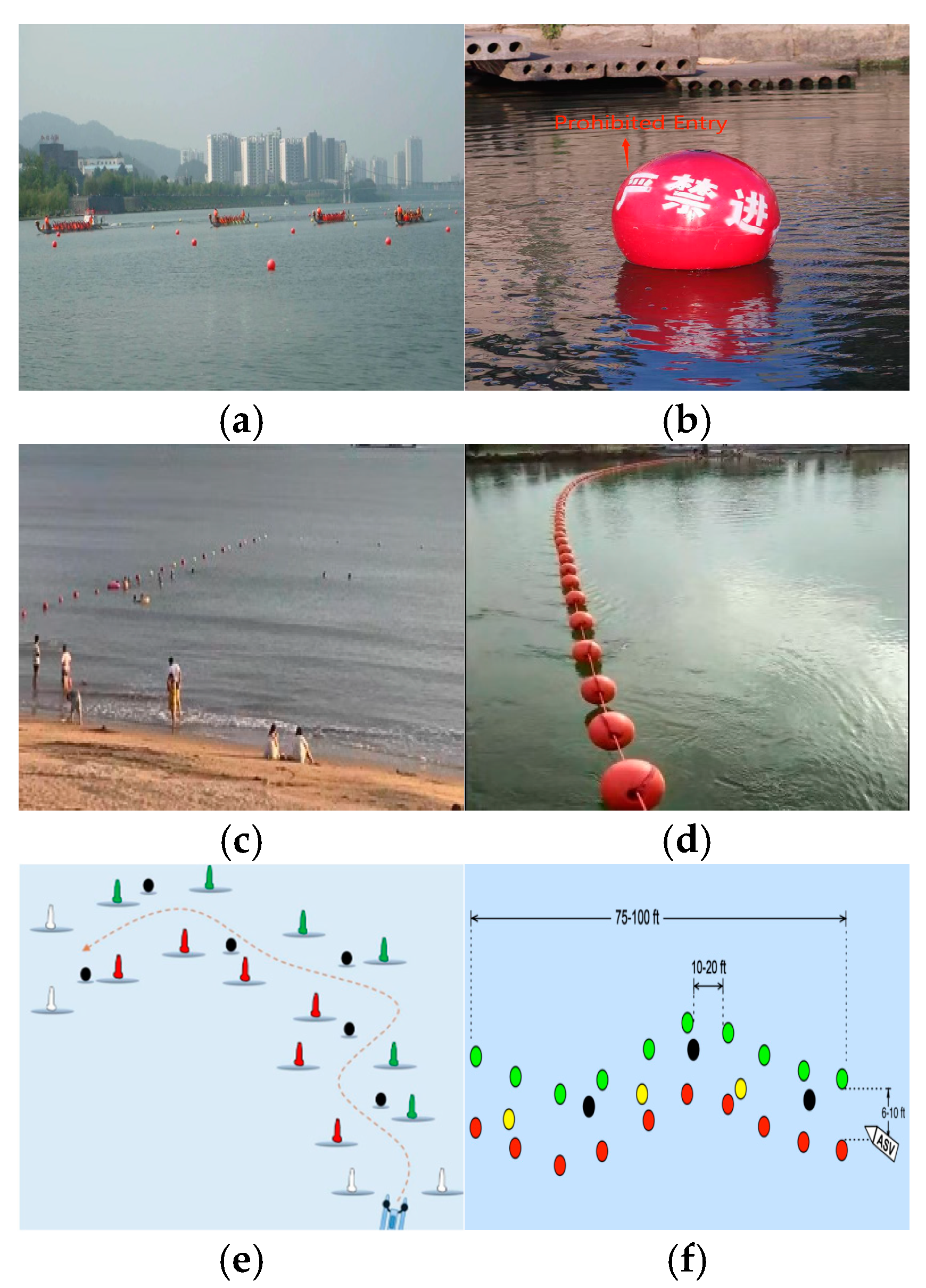
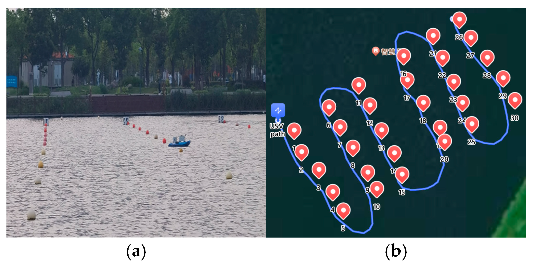
Spherical buoys, serving as water surface markers, are widely used in scenarios such as dragon boat racing course markers, hazard warnings for water bodies, swimming area demarcations, and aquaculture region delineations (Figure 1a–d). Accurate positional information of these buoys can assist USV in precisely identifying navigation channels and hazardous areas, thereby optimizing their navigation routes. Additionally, using spherical buoys as reference points can help them correct their own positions and improve navigation accuracy. Furthermore, spherical buoys can be used to measure water flow velocity [1] and assess the impact of ocean currents on wave buoy measurements [2], with the premise being the accurate determination of the spherical buoys’ positions. In recent years, the “RobotX” international maritime challenge has required USVs to navigate within designated paths while avoiding collisions with gateways formed by paired buoys and black spherical buoys randomly placed, as shown in Figure 1e [3,4]. Similarly, in the “Roboboat” international autonomous boat competition, USVs face similar tasks, as shown in Figure 1f, where they must autonomously traverse courses marked by spherical buoys and navigate through obstacles consisting of spherical buoys with a variety of colors [5,6].
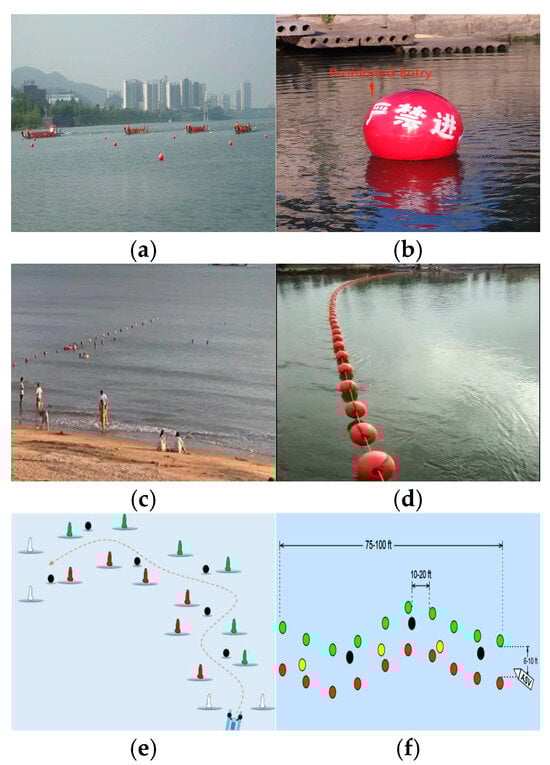
Figure 1.
Application scenarios of spherical buoys. (a) Dragon boat racing course markers. (b) Hazard warnings for water bodies. (c) Swimming area demarcation. (d) Aquaculture region delineations. (e) “RobotX” competition task 3. (f) “Roboboat” competition task 2.
Currently, spherical target localization methods are primarily divided into two categories: fusion of vision and LiDAR and pure vision. Woo et al. [7] used LiDAR to obtain the position information of spherical buoys and combined it with images from a monocular camera. They detected spherical buoys using the Adaboost algorithm and determined their colors based on the Euclidean distance between the HSV values of the detected buoys and reference values. Stanislas et al. [8] built maps using LiDAR data, extracted obstacle lists from these maps, and classified features using a random forest algorithm. They also used HSV color space to determine the color of spherical buoys from images captured by a monocular camera. Although these methods can utilize the high localization accuracy of LiDAR and cameras to obtain position and feature information of spherical buoys, they require precise calibration between LiDAR and cameras. Moreover, feature point matching is challenging in dynamic water environments, which imposes higher demands on system performance. Pure vision-based spherical buoy localization methods are mainly divided into monocular and binocular vision localization. Binocular vision can directly obtain depth information and achieve high localization accuracy [9,10]. However, due to the reflection and water obstruction of spherical buoys on the water surface and the influence of wind and waves causing image tilt during navigation, binocular vision localization faces difficulties in matching and has a large computational load. In contrast, monocular vision localization can effectively avoid these issues. This method requires only one camera and can obtain depth information of targets in images to some extent, featuring a simple structure and fast computation speed [11,12,13].
Regarding the monocular vision-based localization of spherical targets, Penne et al. [14] proposed an analytical method that calculates the center of the sphere using the unique positive real solution of a cubic equation. This method is applicable when the spherical projection forms a complete ellipse. Van et al. [15] utilized monocular camera calibration information and the known actual diameter of the sphere to predict the pixel diameter of the sphere in the image using a small convolutional neural network. They then converted this into three-dimensional coordinates to achieve localization of the sphere. This method can be used to determine the accurate position of a basketball during shooting. Hajder et al. [16] precisely estimated the center position of a sphere in three-dimensional space by detecting ellipses from calibrated camera images and using the known radius of the sphere. This method is suitable for target localization in robotic vision. Zhao et al. [17] improved localization accuracy by combining elliptical projection transformation and experimental site correction techniques. They used data from two identical monocular cameras capturing the trajectory of a sphere (such as a ping-pong ball) and jointly corrected it with experimental site data. This method was designed for automatic hitting robots to quickly identify and locate ping-pong balls during high-speed continuous motion. Budiharto et al. [18] placed the sphere on the camera’s optical axis and estimated the distance between the camera and the sphere using the camera’s tilt angle. This system is primarily applied to soccer robots for ball localization during matches. Guan et al. [19] calculated the three-dimensional coordinates of the sphere’s center in the camera coordinate system based on the projected area and centroid of the sphere extracted from images, combined with the known radius of the sphere and camera internal parameters. They used geometric relationships and similar triangles to achieve this. This method is suitable for three-dimensional localization of spheres in indoor environments.
The above monocular vision localization methods can achieve three-dimensional positioning when the spherical projection contour is complete. However, the positioning of spherical buoys in a water environment faces multiple challenges:
- (1)
- Water obstruction can cause partial loss of the target’s edge, compromising the integrity of the spherical contour;
- (2)
- Water surface reflections can lead to false detection, introducing pseudo-edge points into the target contour;
- (3)
- Changes in illumination affect the grayscale distribution of the image, further weakening the visual distinction between reflections and the actual buoy. Additionally, intense illumination may cause overexposure on the surface of the spherical buoy, weakening local edge features and affecting contour extraction.
Given these challenges, to achieve accurate positioning of spherical buoys using monocular vision in a water environment, two key prerequisites must be met: first, accurately detecting the spherical buoy, and second, reconstructing the contour of the buoy based on the detection.
Current visual-based water surface buoy detection methods are mainly divided into two directions: deep learning-based methods and traditional image processing methods. For water surface buoy detection based on deep learning, Liu et al. [20] proposed an improved YOLOv4 model by integrating reverse depth separable convolution to optimize the network structure. Zhao et al. [21] presented a method combining image enhancement with YOLOv7 for buoy detection. Kang et al. [22] built a detection model based on the YOLOv5 algorithm, using Mosaic data augmentation and feature fusion network technology. Zhang et al. [23] proposed a method based on improved Faster R-CNN for detecting floating objects on the water surface. Zhang et al. [24] presented a method based on improved RefineDet for water surface target detection. However, these methods only generate bounding boxes for detected targets and do not extract their contours. Moreover, they often require the integration of multi-sensor data (such as LiDAR) or the use of stereo cameras to obtain the three-dimensional position information of the buoys. This paper aims to use a more economical monocular vision approach to detect the position of spherical buoys, making the aforementioned deep learning-based detection methods unsuitable for our research scenario.
In deep learning methods, research focused on extracting target contours is mainly concentrated in the field of edge detection. Relevant studies include the following: Cao et al. [25] proposed a new deep refinement network in 2021, combining multiple refinement aspects to obtain substantial edge detection features; Huan et al. [26] proposed a context-aware tracking strategy (CATS) for edge detection; Lin et al. [27] proposed a lateral refinement network algorithm for extracting target edges; Liu et al. [28] designed a fully convolutional neural network based on structural features of each layer for contour extraction; Khan et al. [29] automatically learned to extract image color, geometric features, and edge information to remove pseudo-edge points from contours; and Zheng et al. [30] utilized a convolutional residual neural network, inputted the global image, and combined semantic information for model training, enabling the trained model to detect and locate pseudo-edge points in contours. Although these methods effectively extract target contours and remove pseudo-edge points, they have limitations in our research scenario: they struggle to effectively restore contours lost due to water obstruction and have limited effectiveness in handling local edge feature weakening caused by strong illumination.
Furthermore, whether it is object detection or edge detection based on deep learning, these methods require a large amount of manually annotated training data and depend on multiple rounds of network training. They often require high-performance computing hardware, making it difficult to deploy them effectively on resource-constrained onboard computing platforms.
In contrast, traditional image processing methods are more practical in resource-constrained scenarios due to their simplicity. Aqthobilrobbany et al. [31] proposes a self-navigating system for robotic boats based on HSV color space, achieving visual tracking of spherical buoys through color threshold segmentation. Tran et al. [32] developed a buoy detection system using circular Hough transformation, integrating shape and color features to reduce the interference of illumination changes while maintaining real-time processing capabilities, suitable for automated maritime navigation tasks. However, these traditional methods do not involve contour extraction.
In traditional methods involving contour extraction, relevant research include the following: Shafiabadi et al. [33] used Canny and Sobel filters to detect crack contours in images for analyzing wall cracks; Isar et al. [34] used a denoising system based on the hyperanalytic wavelet transform before edge detection to enhance robustness; Dwivedi et al. [35] used continuous wavelet transformation to detect edge-forming streamlines; Li et al. [36] proposed a method for fitting edge points based on grayscale centroids and moving least squares; and Chen et al. [37] combined wavelet transformation with cubic B-spline interpolation to achieve higher precision in edge detection. However, these traditional contour extraction methods have limitations in our scenario: they cannot effectively remove pseudo-edge points from contours, and they struggle to restore missing contour parts caused by water obstruction. Additionally, they have limited effectiveness in handling local edge feature weakening caused by strong illumination.
To address the above issues, this paper proposes a spherical buoy localization method based on ellipse fitting using monocular vision. The method first preprocesses images of spherical buoys captured by a camera to extract edge points. Then, based on the extracted edge points, it uses grayscale feature analysis for preliminary screening to remove some pseudo-edge points, reducing the number of pseudo-edge points in the input data for Random Sample Consensus (RANSAC). It then uses RANSAC to perform a second screening on the remaining edge points to further eliminate pseudo-edge points. After that, it uses the least squares method to fit an ellipse to the screened edge points, obtaining high-precision ellipse parameters. Finally, based on the ellipse parameters, this paper establishes a monocular vision-based spherical buoy localization model. The model converts the position of the spherical buoy in the world coordinate system into pixel coordinates using a pinhole camera model and calculates the Euclidean distance from the endpoints of the projected ellipse’s major axes to the camera’s optical axes center. It normalizes these distances with the camera’s focal length and applies the arctangent function to calculate the corresponding viewing angles. By determining the angle difference, it uses the known radius of the spherical buoy and geometric relationships to solve the relative distance between the spherical buoy and the camera. Based on relative distances and the USV’s position from satellite observation in the scene, we estimated the precise location of the spherical buoy in space, achieving global positioning of the spherical buoy.
The main contributions of this paper are summarized as follows:
- A monocular vision-based localization method using elliptical fitting is proposed to address the issues of partial edge loss caused by water obstruction and the weakening of local edge features due to strong light, thereby improving the positioning accuracy of spherical buoys in environments with water obstruction and high illumination.
- A multi-step pseudo-edge elimination method for elliptical fitting is proposed to solve the problem of reflection interference. By performing multi-step edge point filtering on images, this method effectively reduces the impact of reflections and other interferences on elliptical fitting.
- Experimental verification was conducted. Through experiments, the effectiveness and accuracy of this method in real-world environments were validated, demonstrating its practical value in the localization of spherical buoys on the water surface.
The remainder of this paper is organized as follows: Section 2 describes the image preprocessing process; Section 3 presents the monocular vision localization method based on ellipse fitting; Section 4 provides simulation verification; Section 5 presents shipboard verification; and Section 6 concludes the paper.
2. Image Preprocessing
Figure 2 illustrates the image preprocessing process for spherical buoys. In real-world environments, images captured by a USV can result in the objects on the water surface and their reflections appearing tilted relative to the pixel coordinate system’s vertical axes due to the roll angle. To correct this tilt, this paper uses an inertial measurement unit (IMU) to measure the roll angle of the USV and applies an image rotation algorithm to correct the image.
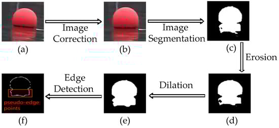
Figure 2.
Image preprocessing process. (a) Original image. (b) Corrected image. (c) Binary image. (d) Eroded image. (e) Dilated image. (f) Edge detection result.
Assuming the rotation center is the origin of the pixel coordinate system, the pixel coordinates before correction are denoted as , the roll angle is denoted as , and the corrected pixel coordinates are given by:
Using the inverse mapping method, the rotated pixel points are determined according to the mapping relationship to correct the original pixel points. The corrected image is shown in Figure 2b.
Let the corrected RGB image be denoted as follows:
Based on the environmental and color information of the spherical buoys, the image is segmented to obtain the binary image of the spherical buoys. The segmentation strategy is expressed as follows:
where, , , and represent the coefficients of the three channels used to adjust the intensity of different color channels. Their values are positive or negative depending on the color of the spherical buoys. For example, for red spherical buoys, is positive, while and are negative.
After target segmentation processing, a binary image is obtained, as shown in Figure 2c. However, the image contains noise and holes, which affect subsequent detection and reduce the detection rate of the spherical buoys. To solve this problem, this paper uses morphological opening processing. A circular structural element with a radius of 4 is selected to first erode and remove noise and then dilate to fill gaps, as follows:
The binary Figure 2e obtained from the above processing contains spherical buoys and their reflections. Since there are often multiple spherical buoys in the image, based on 8-connectivity, connected region labeling is performed on the regions of the spherical buoys and their reflections to distinguish between different buoys. Then, the Canny edge operator is used to extract the edges of each spherical buoy, with the extraction results shown in Figure 2f.
3. Monocular Vision-Based Localization Method Using Elliptical Fitting
Based on the edge points generated from the image preprocessing in the previous section, this section further explores the localization method for spherical buoys. The structure of the monocular vision localization system is shown in Figure 3. Due to the obstruction caused by water, which results in incomplete contours of the spherical buoys, a localization method based on ellipse fitting is proposed. This method leverages the characteristic that the projection of a sphere in a camera appears as a circle or an ellipse [14].
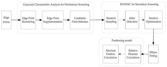
Figure 3.
Monocular vision localization system structure.
3.1. Obtaining Ellipse Parameters
In water environments, the presence of water surface reflections often results in a large number of pseudo-edge points among the obtained edge points. These pseudo-edge points significantly affect the accuracy of ellipse fitting using the least squares method, leading to biases in the estimation of ellipse parameters such as the center and radius, which in turn impact the localization accuracy of spherical buoys. Therefore, accurately estimating ellipse parameters is crucial.
RANSAC is a robust algorithm used to estimate mathematical model parameters from data containing outliers [38]. Its core idea is to find the model that best represents the data through random sampling and inlier detection. However, when the proportion of pseudo-edge points is high, RANSAC’s performance significantly deteriorates because random sampling is more likely to select pseudo-edge points, resulting in inaccurate ellipse model estimation.
In addition to considering the ellipse model, this paper also starts from the actual scenario of water surface spherical buoys. It uses the different grayscale values between the spherical buoy area and the reflection area to perform grayscale characteristic analysis on the reflection boundary line area, thereby determining the position of the reflection boundary line. However, in practical applications, changes in lighting conditions significantly affect the grayscale distribution of images, leading to a reduction in the grayscale value differences in the reflection boundary line area, which in turn affects the accurate positioning of the reflection boundary line.
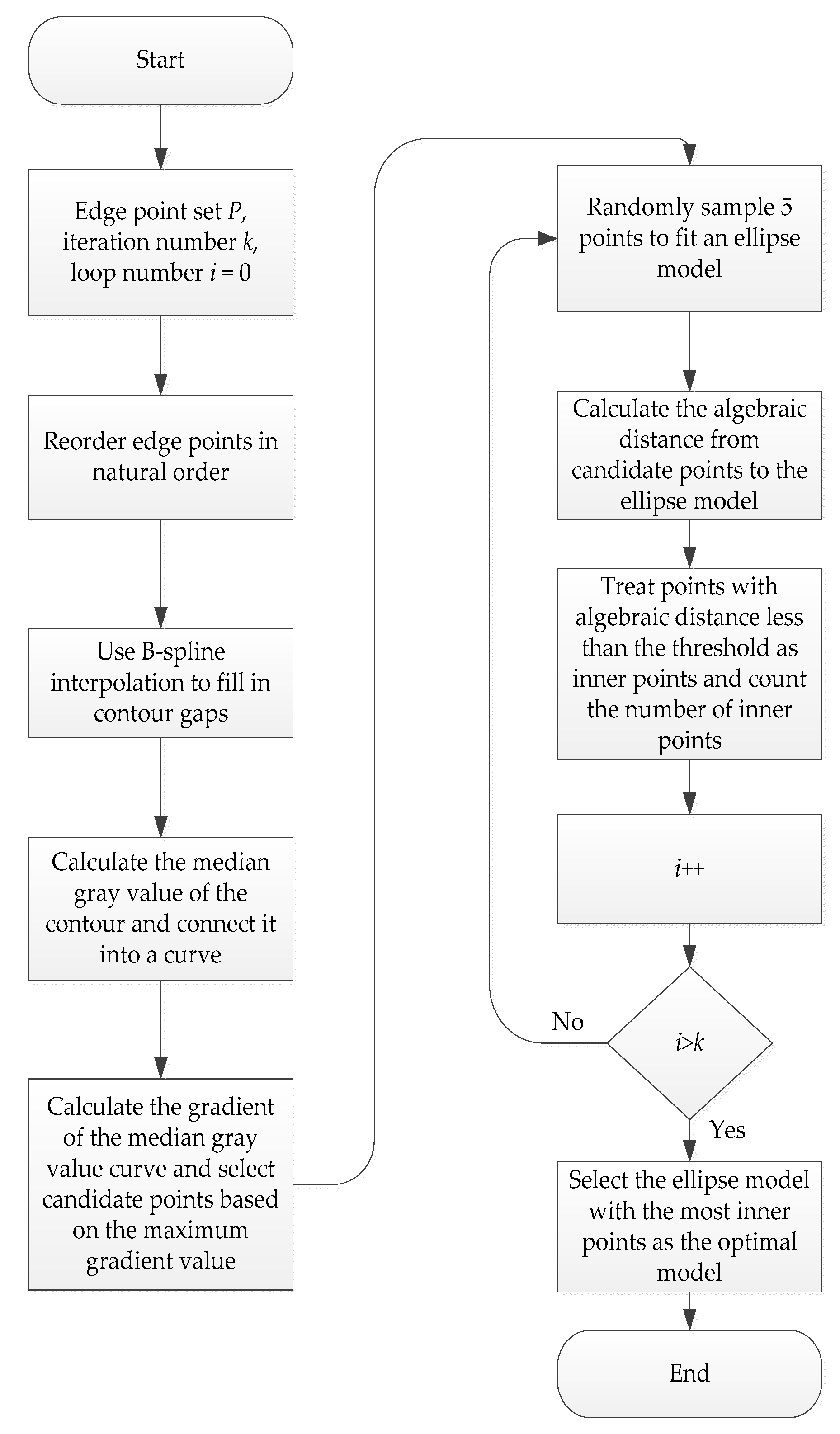
Since using grayscale analysis or RANSAC alone has limitations, this paper proposes a multi-step pseudo-edge removal ellipse fitting method. This method first uses grayscale analysis to preliminarily screen edge points and remove some pseudo-edge points, thereby reducing the number of pseudo-edge points input into RANSAC. Then, it uses RANSAC to perform a second screening on the remaining edge points to further eliminate pseudo-edge points. Finally, it uses the least squares method to fit an ellipse to the screened edge points, obtaining high-precision ellipse parameters. Figure 4 illustrates the process, and the specific steps are as follows:
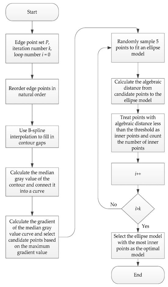
Figure 4.
Algorithm flowchart.
- (1)
- Edge Point Reordering
Let the set of detected edge points be , where represents the coordinates of the th edge point. These points are reordered according to the natural order of the ellipse (clockwise or counterclockwise) to obtain a new ordered set .
- (2)
- Edge Point Supplementation
Due to the possibility that image preprocessing may not fully extract the target edge contour, resulting in gaps in the contour, a set of points is defined for the missing regions. Through B-spline interpolation, a set of supplementary points is generated. The mathematical expression for the B-spline is as follows:
where is the B-spline curve; represents the control points selected from the ordered set ; is the th B-spline basis function; is the order of the B-spline; and is the parameterization variable. By using B-spline interpolation to generate the supplementary point set and by merging it with the original point set , the following closed contour is constructed:
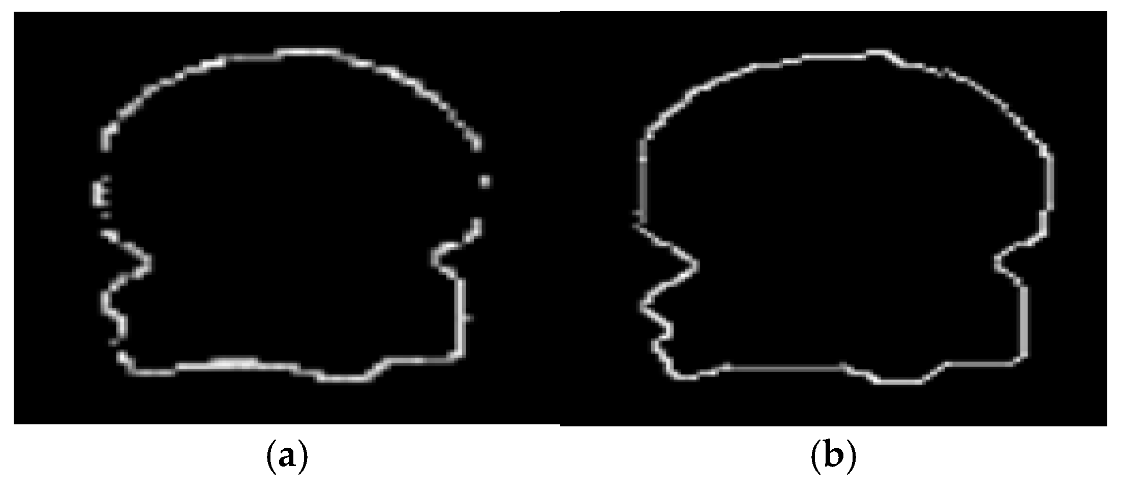
The constructed closed contour is shown in Figure 5:
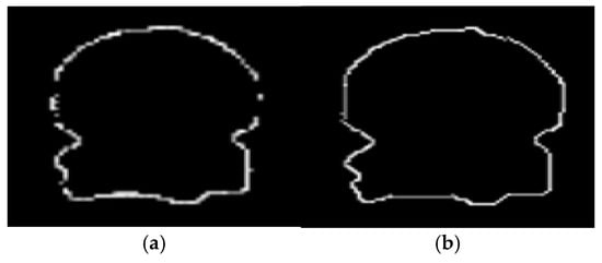
Figure 5.
Constructing a closed contour. (a) Contour gap diagram. (b) Closed contour diagram.
- (3)
- Candidate Point Selection
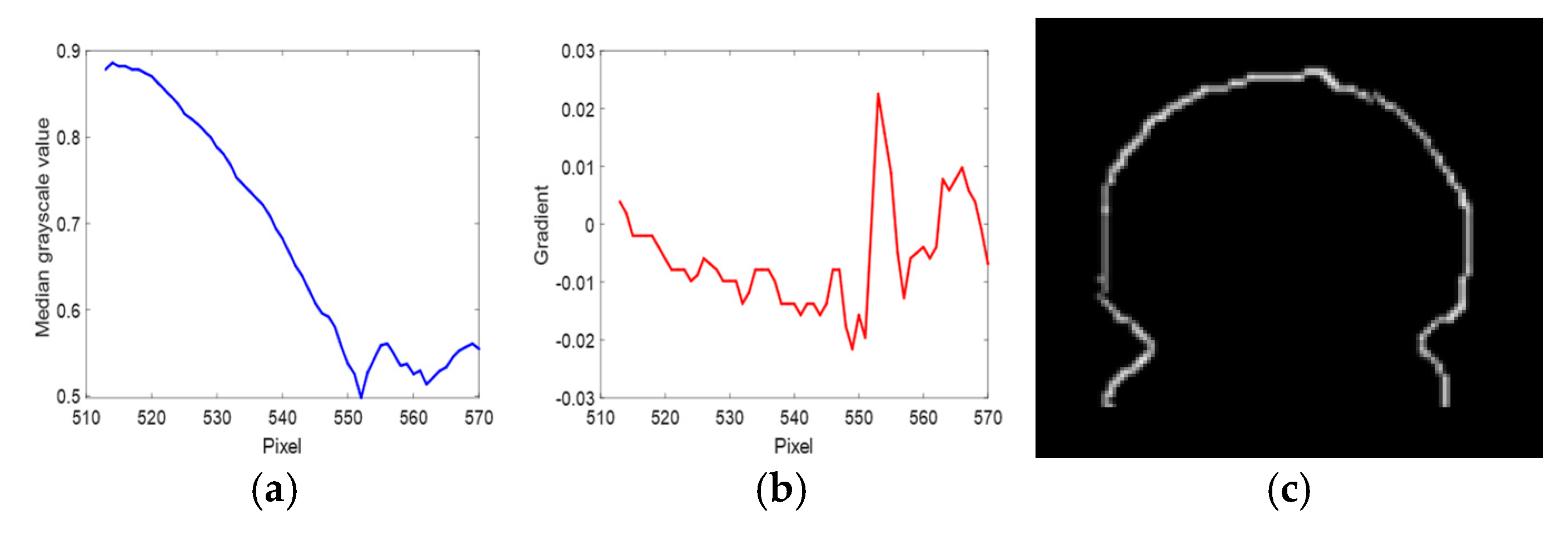
Let the grayscale value of each row in the image be , where is the row number and is the image width. For the closed contour , extract the pixel grayscale value of each row within the contour via the following expression:
Calculate the median grayscale value for each row:
Connect the median grayscale values of all rows to form a median grayscale curve , and calculate the gradient of the median grayscale curve :
Find the row number corresponding to the maximum gradient value:
The edge points above the split line are identified as candidate points for the true contour:
The median grayscale curve, gradient curve, and candidate points are shown in Figure 6a–c:
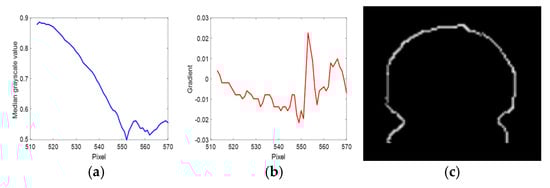
Figure 6.
Related curve diagrams of candidate points. (a) Median grayscale curve. (b) Gradient curve. (c) Candidate points.
- (4)
- Random Sampling
Randomly select five points from the candidate point set , and use the least squares method to fit the ellipse model through the following minimized objective function:
Solve for the ellipse parameters , , , , , and .
- (5)
- Inlier Detection
For each point , calculate its algebraic distance to the ellipse model:
if (preset threshold), it is judged as an inlier; otherwise, it is judged as an outlier. Count the number of inliers of the current ellipse model. If the number of inliers of the current ellipse model is greater than the historical optimal value, update the optimal ellipse model and inlier set.
- (6)
- Iterative Optimization
Repeat the above two steps (random sampling and inlier detection) times. Each iteration generates a candidate ellipse model, and its quality is evaluated by inlier detection. Finally, the ellipse model with the largest number of inliers is selected as the optimal model.
- (7)
- Ellipse Fitting
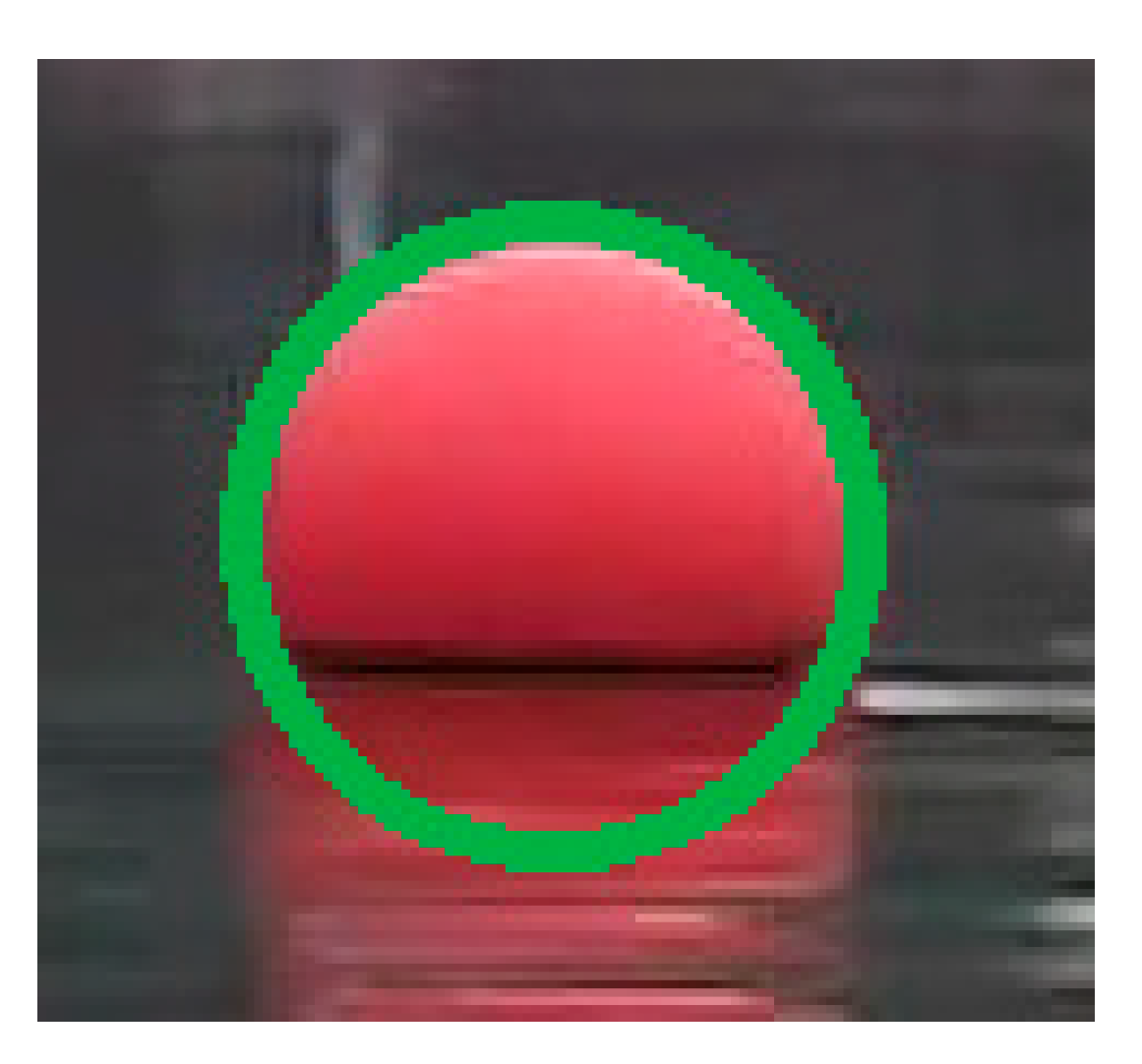
Use the optimal inlier set, and use the least squares method to fit the final ellipse model, as shown in Figure 7:

Figure 7.
Final fitted ellipse (red markers indicate spherical buoy, while green contours represent fitted ellipse).
3.2. Positioning Calculation
Currently, monocular vision ranging methods are mainly divided into three categories [11,12,13]: The first category is to calculate the distance between the camera and the target based on the geometric relationship established by the imaging model; the second category is to calculate the actual distance by establishing the proportional relationship between the actual length of the target and its physical length in the image and then using the principle of triangle similarity; the third category is to measure distance by establishing a mathematical regression model. This paper is based on the first method, establishing a ranging model based on the parameters of the projected ellipse. Building on this, we utilize the known satellite observation data from the USV in the scene to obtain the coordinates of each spherical buoy in the geodetic coordinate system.
3.2.1. Relative Distance Calculation
When the center of the sphere is located on the camera’s optical axis, its projection on the image plane is circular; in other cases, its projection is elliptical. These projected ellipses have the following characteristics [17]:
- The image plane center lies on the line containing the major axes of the ellipse.
- The image point of the center of the sphere is located on the line segment of the major axes of the ellipse.
The pinhole imaging model of the spherical buoy is shown in Figure 8a:
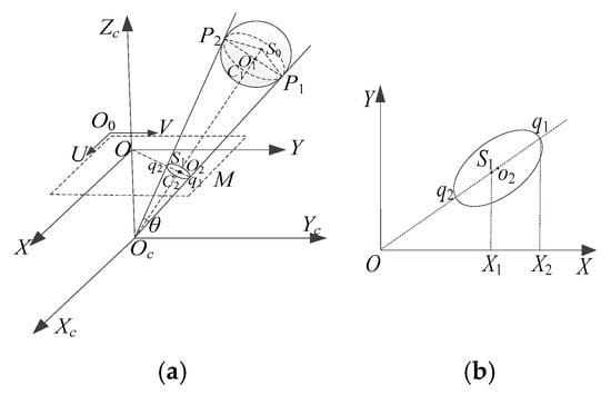
Figure 8.
Spherical buoy imaging model. (a) Pinhole imaging model. (b) Projected ellipse.
Where is the camera coordinate system, is the image coordinate system, and is the pixel coordinate system. and are the endpoints of the major axes of the ellipse formed by the projection of the spherical buoy on the image plane. and are the tangent points where extensions of and intersect the sphere. is the center of the spherical buoy; is the projection of the sphere’s center on the image plane; is the center of the projected ellipse; and is the angle formed by , , and the origin of the camera coordinate system.
Using the pinhole camera model to transform world coordinates to pixel coordinates , the transformation expression is as follows:
where is the camera focal length; and are the physical dimensions of a single pixel in the and axes directions, respectively; are the pixel coordinates of the image plane center; and represent the rotation matrix and translation vector from the world coordinate system to the camera coordinate system, respectively; and is the depth coordinate value of the spherical buoy in the camera coordinate system. Let the camera intrinsic parameter matrix be:
where , represent the effective pixel focal lengths in the -axis and -axis directions of the image, respectively. Let the extrinsic parameter matrix be , so we can obtain the following:
Ignoring camera distortion and other factors, the projection of the spherical buoy is always perpendicular to the line connecting the sphere’s center to the camera’s optical center. The points where rays emitted from are tangent to the sphere form a circle . These rays and form a right circular cone with as its vertex. According to the above geometric relationships, we can obtain:
where are the pixel coordinates of , and are the pixel coordinates of . Since is a tangent point on the sphere, according to the properties of tangents to a circle, is perpendicular to , and is the angle bisector of . Let the radius of the spherical buoy be , then the distance from the sphere’s center to the origin of the camera coordinate system is as follows:
3.2.2. Estimate the Spherical Buoy’s Coordinates in the Geodetic Coordinate System
Since the projection point of the sphere center on the image plane coincides with the center of the ellipse only when the sphere center is on the optical axes of the camera, and and do not coincide in other cases, cannot be directly regarded as the projection point of the sphere center. Based on the property that is the angular bisector of , Equations (17) and (18) can be combined to obtain:
Since points , , and are collinear, and are projected onto the axes of the image coordinate system, forming two similar triangles. As shown in Figure 8b, and are the projections of and onto the axes, respectively. By the theorem of similar triangles, the pixel coordinates of can be obtained:
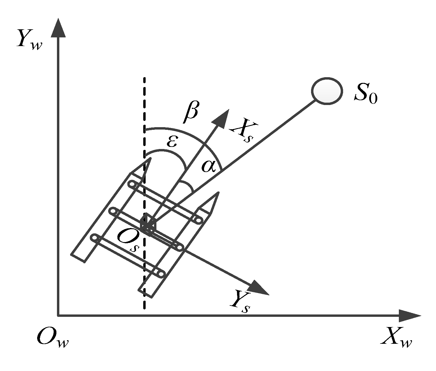
Estimate the spherical buoy’s coordinates in the geodetic coordinate system using the relative distance between the camera coordinate system’s origin and the sphere’s center, the USV’s position from satellite observation, and the heading information. As shown in Figure 9, the positional relationship between the spherical buoy and the USV is established. represents the world coordinate system; represents the body coordinate system of the vehicle, where the origin is the center of gravity of the USV; is the angle between the line connecting the center of the sphere and the center of gravity of the USV and the axes of the world coordinate system; is the angle between the axes of the body coordinate system and the axes of the world coordinate system, which is the heading angle of the USV; and is the angle between the line connecting the center of the sphere and the center of gravity of the USV and the axes of the body coordinate system:

Figure 9.
Positional relationship.
Assuming the body frame coincides with the camera frame and the USV’s position from satellite observation is , the estimated coordinates of the spherical buoy in the geodetic coordinate system are obtained as:
where is the vertical distance from the camera’s optical center to the horizontal plane containing the center of the sphere.
4. Simulation Verification
4.1. Scene Simulation
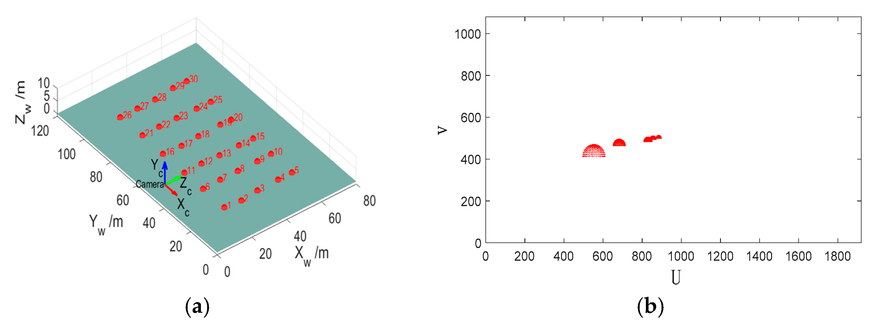
To verify the accuracy of the proposed localization method in this paper, simulation experiments were conducted under different conditions and compared with the method in reference [19]. The simulation scenario is shown in Figure 10, where Figure 10a is a three-dimensional scene in which 30 spherical buoys are arranged in five rows and six columns; the red, blue, and green arrows represent the , , and axes of the camera coordinate system, respectively. The projection of the spherical buoys obtained by the camera located in the position shown in Figure 10a is shown in Figure 10b.

Figure 10.
Simulation scenario. (a) 3D scene. (b) Projection diagram.
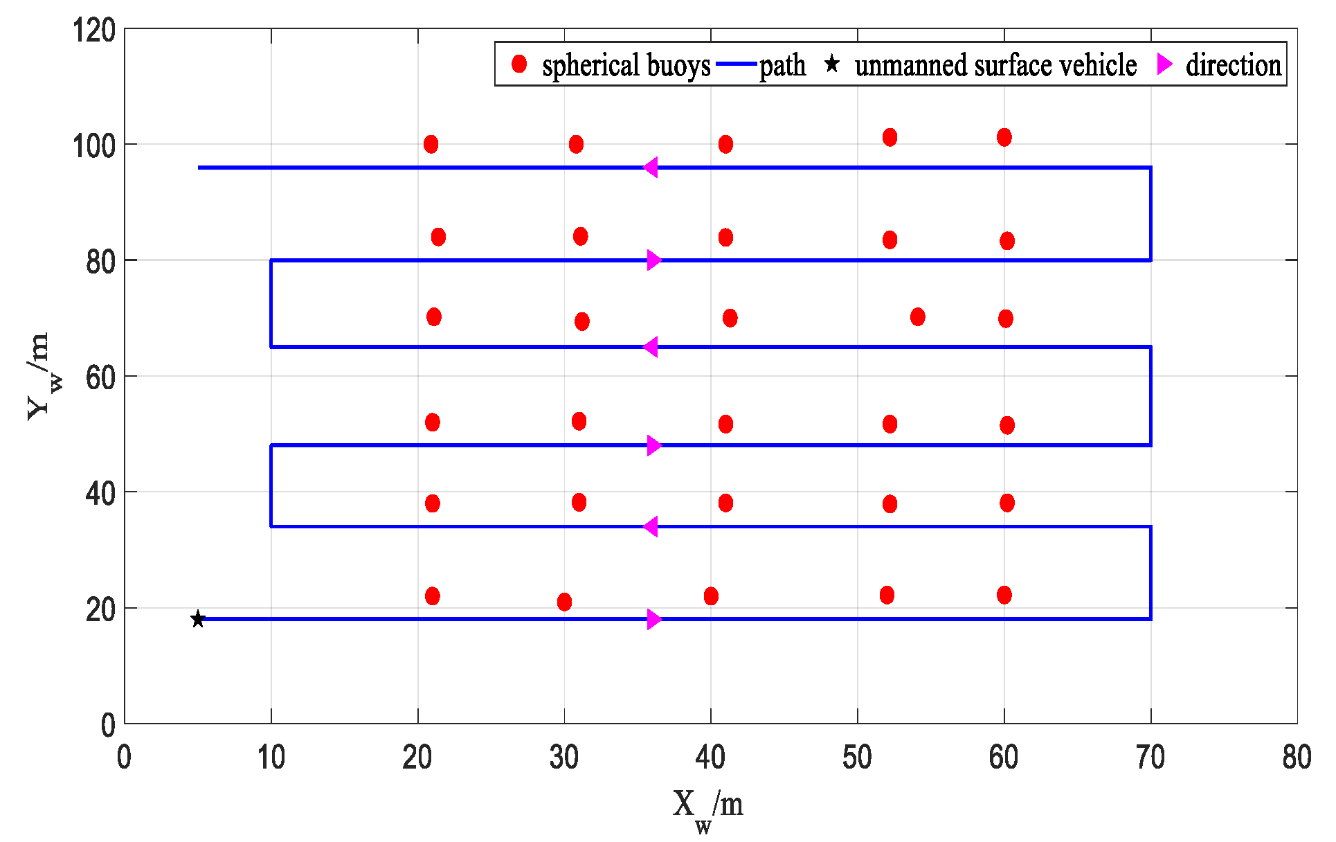
To ensure that the camera mounted on the USV can effectively capture the spherical buoys along its path during the defined route, the simulation experiment path is set as shown in Figure 11. In the experiment, the initial coordinates of the USV are set to (5, 18), and the initial heading angle is set to 0 degrees. As the USV travels along the defined path, every 1 m, a coordinate calculation is performed for each spherical buoy appearing in the projection image, and the total number of times each spherical buoy appears in the projection image is recorded as , as well as the result of each coordinate calculation , where represents the spherical buoy number, , . Then, based on the frequency of appearance of each spherical buoy and the results of each coordinate calculation, the mean of its coordinates is computed and used as the estimated coordinate value of the spherical buoy in the geodetic coordinate system:
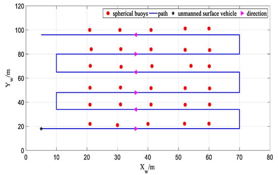
Figure 11.
Simulation path.
To evaluate the accuracy of the localization method, the mean absolute error is used as an intuitive metric:
where represents the true coordinates of the spherical buoy in the geodetic coordinate system.
4.2. Impact of Noise Interference
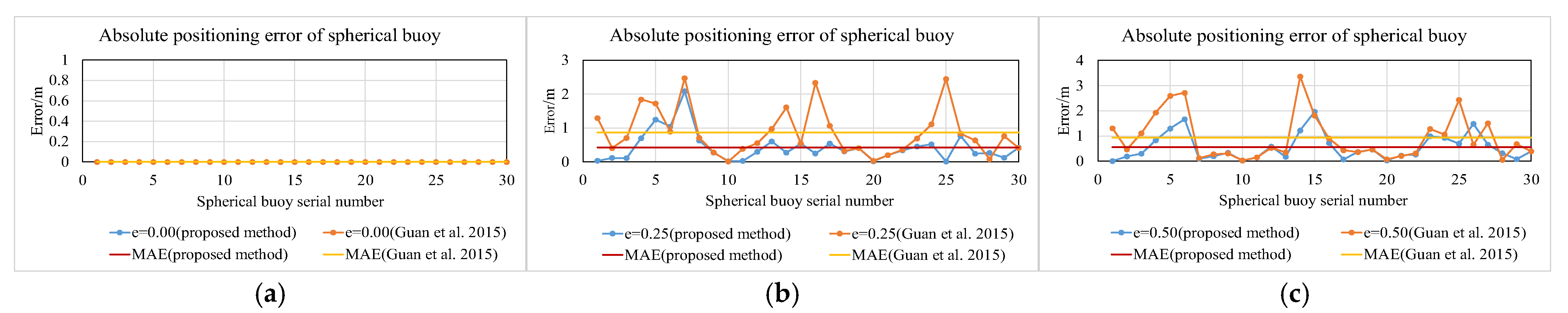
The projection of the spherical buoy is subject to interference from environmental and image processing parameters, and the combined effect of these factors may lead to errors in extracting the feature parameters of the spherical buoy. To simulate the effects of these disturbances, the camera focal length was set to 12mm and the camera height was set to 30cm in the simulation experiment, and comparative experiments were conducted with different pixel noise intensities. A noise level of 0.00 was selected to simulate the case of no pixel noise to verify the correctness of the method in this paper. In addition, noise levels of 0.25 and 0.50 were selected to simulate the interference of small and moderate pixel noise, respectively, to test the anti-interference ability of the method in this paper. The results of the simulation experiments are shown in Figure 12a–c.
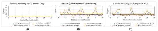
Figure 12.
Impact of noise interference (proposed method vs. Guan et al. [19]). (a) Absolute error with noise at 0.00. (b) Absolute error with noise at 0.25. (c) Absolute error with noise at 0.50.
Figure 12a–c show the simulation experiment results using the method from reference [19] and the method presented in this paper under different noise intensities. As can be seen from the figures, under the condition of 0.00 noise, the mean absolute error calculated by both methods is 0, indicating that both methods can correctly calculate the absolute coordinates without noise interference, which verifies the correctness of the method in this paper. However, as the noise increases, the mean absolute error calculated by both methods increases. This is because as the pixel noise increases, the proportion of pixel noise in the projection area of the spherical buoy increases. Therefore, the influence of pixel noise on the absolute coordinate solution gradually increases, and the mean absolute error obtained by solving the absolute coordinates also gradually increases. Under the conditions of 0.25 and 0.50 noise, the mean absolute errors obtained by the method in reference [19] are 0.86 m and 0.93 m, respectively, while the mean absolute errors obtained by the method in this paper are 0.42 m and 0.56 m, respectively. The mean absolute error is reduced by 51.1% and 39.7%, respectively, which verifies the anti-interference effect of the method in this paper.
4.3. Impact of Camera Height
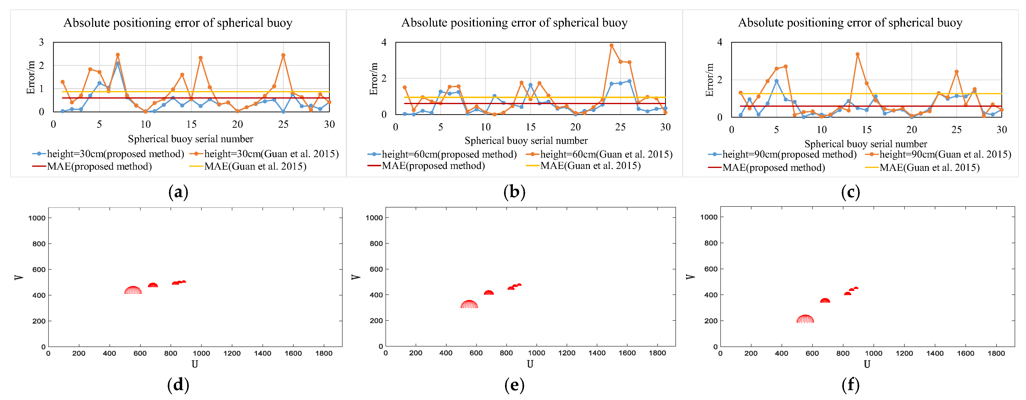
To verify the influence of camera height on the algorithm in this paper, the camera focal length was set to 12 mm and the noise was set to 0.25 in the simulation. Comparative experiments were conducted with camera heights of 30 cm, 60 cm, and 90 cm. The results of the simulation experiments are shown in Figure 13a–f.
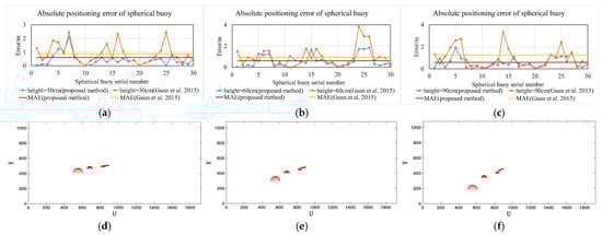
Figure 13.
Impact of camera height (proposed method vs. Guan et al. [19]). (a) Absolute error at 30 cm height. (b) Absolute error at 60 cm height. (c) Absolute error at 90 cm height. (d) Projection at 30 cm height. (e) Projection at 60 cm height. (f) Projection at 90 cm height.
Figure 13a–c show the simulation experiment results obtained using the two methods at different camera heights. As can be seen from the figures, as the camera height increases, the mean absolute error obtained using the method in this paper stabilizes within 0.62 m, while the mean absolute error obtained using the method in reference [19] increases. Furthermore, at the same height, the mean absolute error obtained using the method in this paper is reduced by more than 30.6% compared to the method in reference [19]. It can be seen that the method in this paper is more stable and accurate in locating spherical buoys at different camera heights.
Figure 13d–f represent the projection situations when the camera height is 30 cm, 60 cm, and 90 cm, respectively. As can be seen from the figures, as the camera height increases, the projection area of the spherical buoy in the camera gradually decreases; at the same time, the occlusion between the spherical buoys in the image decreases, which improves the visibility of the spherical buoys in the image so that a more complete projection shape of the spherical buoys can be obtained. The mean absolute error when using the method in this paper at a camera height of 30 cm is relatively the smallest, which indicates that although increasing the camera height can improve visibility, the reduction in the projection area has a more significant impact on the method in this paper. This also provides a basis for the selection of camera height in real-world experiments.
4.4. Impact of Camera Focal Length
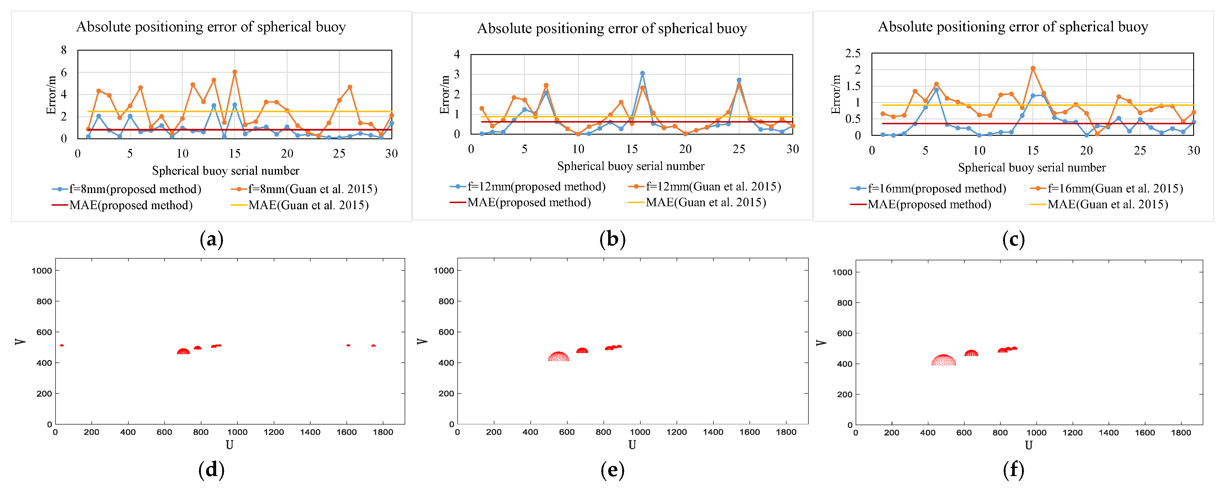
To evaluate the effect of changes in camera focal length on the algorithm in this paper, under the simulation conditions of noise at 0.25 and camera height at 30 cm, the camera focal length was set to 8 mm, 12 mm, and 16 mm, respectively, and the absolute error under different focal lengths was calculated. The simulation results are shown in Figure 14a–f.
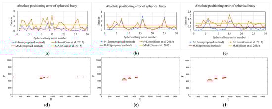
Figure 14.
Impact of focal length (proposed method vs. Guan et al. [19]). (a) Absolute error at 8 mm focal length. (b) Absolute error at 12 mm focal length. (c) Absolute error at 16 mm focal length. (d) Projection at 8 mm focal length. (e) Projection at 12 mm focal length. (f) Projection at 16 mm focal length.
Figure 14a–c show the results of solving the absolute coordinates of the spherical buoys using the two methods at different focal lengths. As can be seen from the figures, when the focal length is 12 mm and 16 mm, the mean absolute error calculated by both methods is less than 1 m. This indicates that both methods can effectively and accurately solve the absolute coordinates when the focal length is 12 mm and 16 mm. However, when the focal length is 8 mm, the mean absolute error obtained by the method from reference [19] is 2.47 m, while the mean absolute error obtained by the method in this paper is 0.81 m. Compared with the method from reference [19], the mean absolute error is reduced by 67.2%, which indicates that the method in this paper has high adaptability under different camera focal length conditions.
Figure 14d–f represent the projection situations when the focal length is 8 mm, 12 mm, and 16 mm, respectively. As can be seen from the figures, as the focal length increases, the proportion of the projected area of the spherical buoy in the image increases. This is because the increase in focal length leads to a decrease in the camera’s field of view, which makes the area of the spherical buoy in the image relatively larger, which will improve the noise resistance of the two methods.
4.5. Impact of Rotation Angle
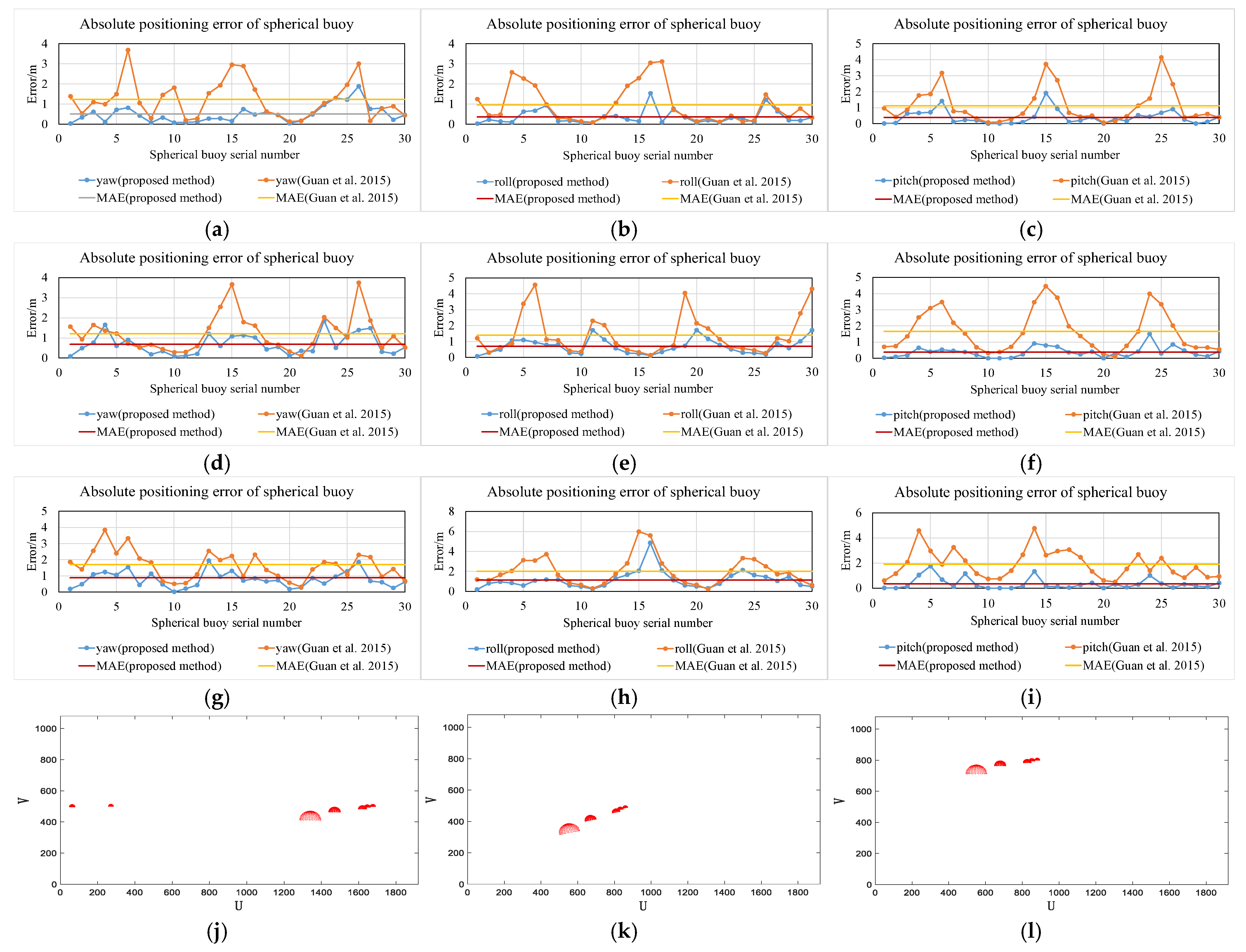
During the operation of the USV, its roll angle, pitch angle, and yaw angle will change. To evaluate the effect of changes in the rotation angle on the algorithm in this paper, the noise was set to 0.25, the focal length was set to 12 mm, and the camera height was set to 30 cm in the simulation. The rotation angles were set to 10°, 20°, and 30°, respectively, and the absolute error under different rotation angle disturbances was calculated. The simulation results are shown in Figure 15a–l.
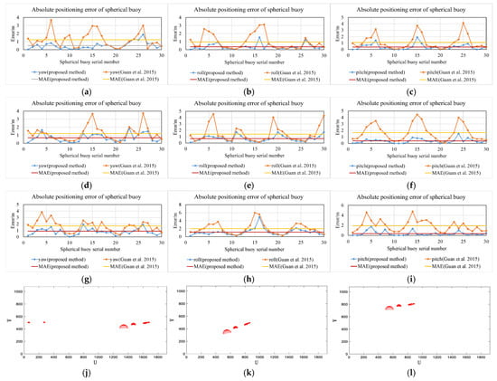
Figure 15.
Impact of rotation angle (proposed method vs. Guan et al. [19]). (a) Absolute error at 10° yaw angle. (b) Absolute error at 10° roll angle. (c) Absolute error at 10° pitch angle. (d) Absolute error at 20° yaw angle. (e) Absolute error at 20° roll angle. (f) Absolute error at 20° pitch angle. (g) Absolute error at 30° yaw angle. (h) Absolute error at 30° roll angle. (i) Absolute error at 30° pitch angle. (j) Projection at 10° yaw angle. (k) Projection at 10° roll angle. (l) Projection at 10° pitch angle.
Figure 15a–i show the results of locating spherical buoys using the two methods when the USV is affected by different magnitudes of yaw, roll, and pitch angles of 10°, 20°, and 30°. As can be seen from the figures, under the influence of rotation angles, the mean absolute error obtained by the method in this paper is smaller, indicating that the absolute coordinates of the spherical buoy obtained based on the method in this paper are closer to the true value. Especially under the influence of the roll angle, when the roll angle reaches 30°, the mean absolute error obtained by the method from reference [19] is 1.99 m, while the mean absolute error obtained by the method in this paper is 1.15 m. Compared with the method from reference [19], the mean absolute error is reduced by 42.2%. Thus, it can be concluded that under the influence of rotational disturbances, the method in this paper has a better absolute coordinate solution effect.
Figure 15j–l represent the projection scenarios when the yaw, roll, and pitch angles are 10 degrees, respectively. As can be seen from the figures, under the influence of the yaw angle, the projected position of the spherical buoy shifts left and right; under the influence of the pitch angle, the projected position of the spherical buoy shifts up and down; under the influence of the roll angle, the spherical buoy appears tilted.
5. Real-World Experiment
5.1. Hardware Configuration
Using the USV as a platform for onboard experiments, a high-resolution industrial camera with a resolution of 1920 × 1080 pixels, a focal length of 12 mm, and a height setting of 30 cm was mounted to capture images of the spherical buoys. Through calibration, the intrinsic parameter matrix and distortion coefficients of the onboard camera were obtained:
5.2. USV Experiment
5.2.1. Ellipse Fitting Comparative Experiment
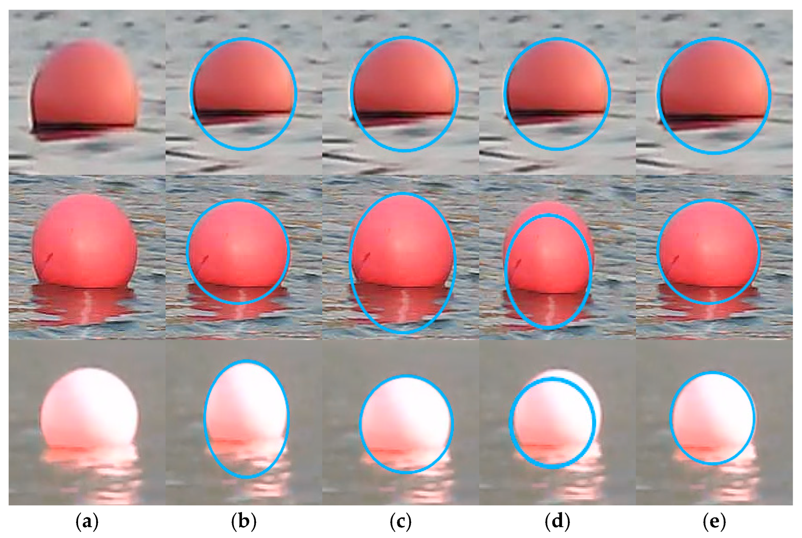
To verify the effectiveness of the ellipse fitting method proposed in this paper, multiple experiments were conducted (with all images captured by the imaging acquisition device carried by USV “Haiyue”). Three representative images were selected for demonstration. Figure 16a shows the original image of the spherical buoy. For these images, we used four different methods to perform ellipse fitting on the edge points of the spherical buoy: the first method filters the edge points based on gray-scale characteristic analysis and uses the least squares method to fit the ellipse, as shown in Figure 16b; the second method uses the RANSAC algorithm to filter the edge points and also uses the least squares method to fit the ellipse, as shown in Figure 16c; the third method applies the constrained randomized Hough transform-based ellipse fitting algorithm proposed in reference [39], as shown in Figure 16d; the fourth method employs the approach proposed in this paper, as shown in Figure 16e.
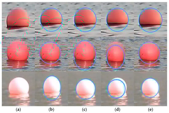
Figure 16.
(a) Original image. (b) Method 1. (c) Method 2. (d) Method 3. (e) Ours.
From the first row of Figure 16, it is evident that all four methods accurately fit the complete spherical buoy contour in the absence of water surface reflections.
In the second row of Figure 16, the larger reflection areas introduce more pseudo-edge points, which compromise the fitting performance of Method 2. This occurs because a higher proportion of pseudo-edge points increases the likelihood of random sampling selecting these erroneous points, leading to inaccurate ellipse model estimates. Method 3 also fails to reconstruct complete contours under reflection interference. In contrast, Method 1 and the method proposed in this paper effectively eliminate reflection interference through grayscale analysis, resulting in more accurate contour fitting.
The third row of Figure 16 shows that under varying illumination conditions, reduced grayscale contrast at reflection boundaries weakens the effectiveness of Method 1. Although Method 3 can filter some curvature anomalies through curvature constraints, it cannot completely remove all pseudo-edge points due to inconsistent curvature distributions introduced by reflections, leading to suboptimal ellipse fitting. Methods 2 and the method proposed in this paper demonstrate improved accuracy when reflection areas are small, as RANSAC effectively filters pseudo-edge points.
In summary, the experimental results validate the effectiveness of the elliptical fitting methods presented in this paper.
5.2.2. Spherical Buoys Localization Experiment
After completing the ellipse fitting comparison experiments, to validate the practicality of the positioning method proposed in this paper, we further conducted a spherical buoy localization experiment on an open lake surface as shown in Figure 17a. The experimental scenario involved 30 spherical buoys with a radius of 12.7 cm, arranged in a 5 × 6 matrix, covering a water surface area of 40 m in width and 80 m in length.
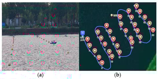
Figure 17.
Spherical buoy localization experiment. (a) Experimental scenario. (b) Trajectory of the USV.
The experiment considered both external and internal interference factors. The external factors primarily refer to varying environmental conditions, while the internal factors pertain to camera distortions. The specific steps of the experiment are as follows: Firstly, a GNSS-equipped USV was manually controlled to visit each spherical buoy in sequence, collecting satellite observation data for each buoy. Subsequently, the USV, equipped with a camera, GNSS, and IMU, traveled along the route set in Figure 17b, synchronously recording image data, the USV’s position from satellite observation, heading information, and roll angle. Finally, the coordinates of each spherical buoy in the geodetic coordinate system were estimated using the method proposed in this paper, as well as the methods presented in references [19,40].
- (1)
- Strong Illumination, Reflections, and Water Obstruction
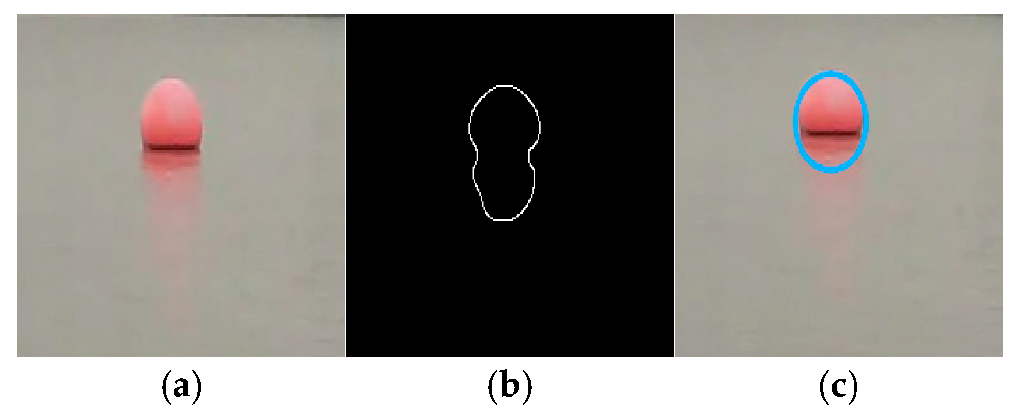
Figure 18a shows an image taken under strong noon illumination, where intense light causes color distortion in parts of the buoy and there are significant reflections and water obstructions. After image preprocessing, the result is shown in Figure 18b, where the contour is affected by false edges and local deformations. Further applying the proposed algorithm for ellipse fitting, the result is shown in Figure 18c. Although there are some contour mismatches, the fitted ellipse aligns well with the actual buoy overall, verifying the algorithm’s robustness against strong illumination.

Figure 18.
Experimental environment: strong illumination, reflections, and water obstruction (red markers indicate spherical buoy, while blue contours represent fitted ellipse). (a) Original image. (b) Preprocessed image. (c) Ellipse fitting result.
In this environment, the comparison of absolute errors among the three methods is shown in Figure 19.
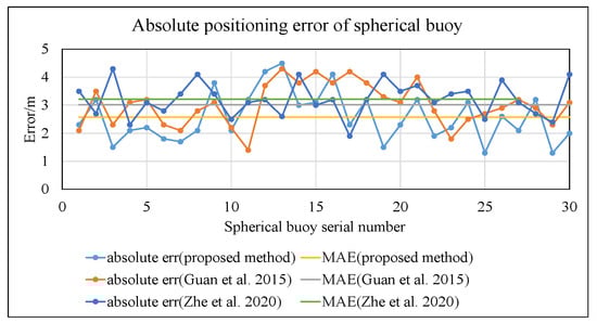
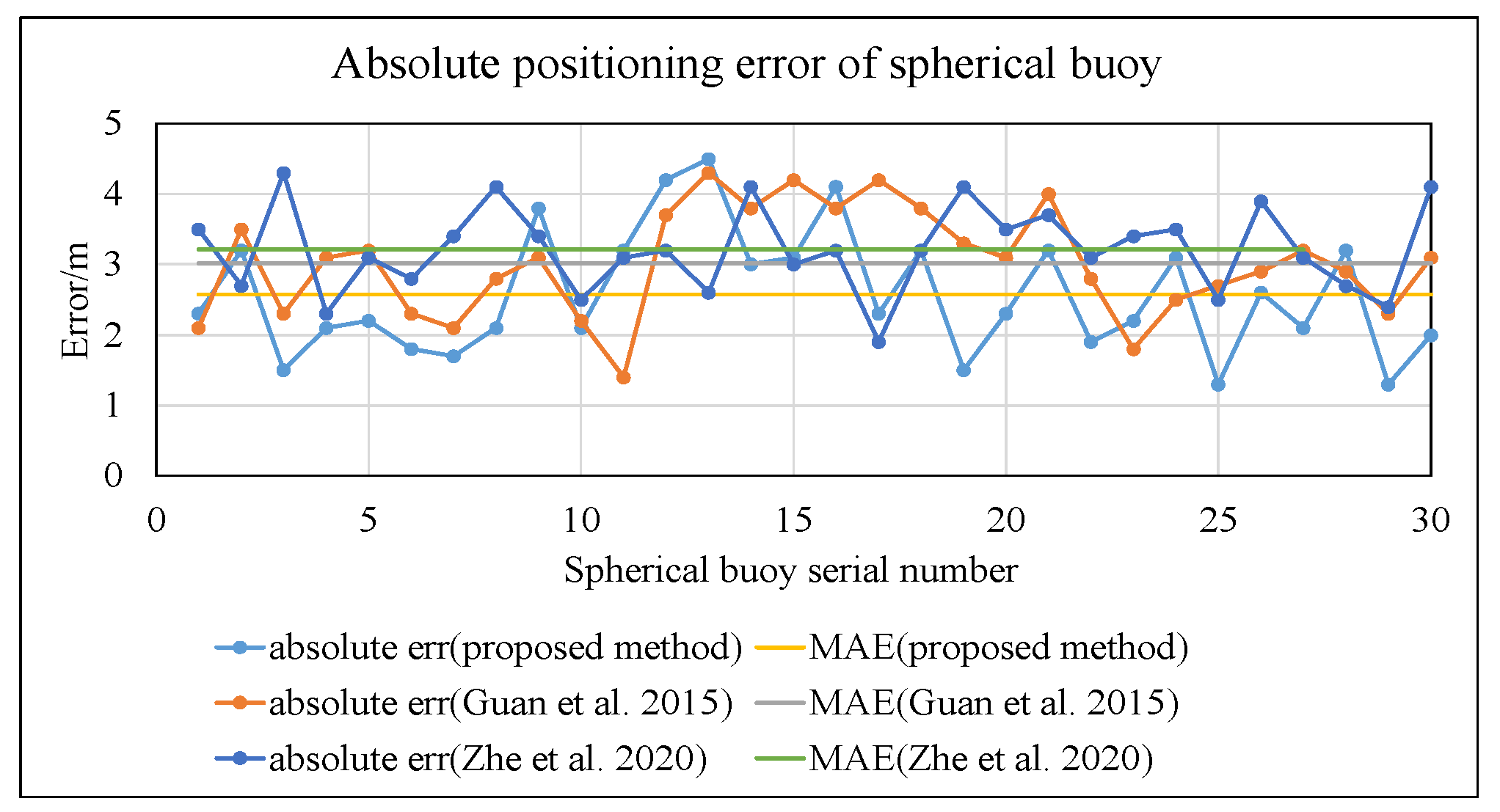
Figure 19.
Comparison chart of positioning results under high illumination, reflection, and water obstruction conditions (proposed method vs. Guan et al. [19] and Zhe et al. [40]).
As shown in Figure 19, the mean absolute error of the spherical buoy positions calculated using the method proposed in this paper is 2.57 m. This represents a reduction of 14.6% compared to the method in reference [19] (3.01 m) and a reduction of 19.9% compared to the method in reference [40] (3.21 m).
- (2)
- Low Illumination, Reflections, and Water Obstruction
Figure 20a shows an image captured in a low-light evening scenario, where illumination intensity is significantly reduced but reflections and obstructions still exist. The preprocessing result is shown in Figure 20b, and the ellipse fitting result is shown in Figure 20c. The detection results indicate that the algorithm can accurately reconstruct the buoy contour even under weak light, reflections, and water obstructions.
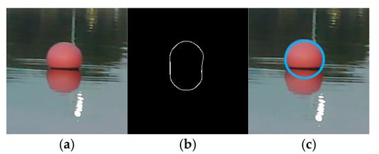
Figure 20.
Experimental environment: low illumination, reflections, and water obstruction (red markers indicate spherical buoy, while blue contours represent fitted ellipse). (a) Original image. (b) Preprocessed image. (c) Ellipse fitting result.
In this environment, the comparison of absolute errors among the three methods is shown in Figure 21.
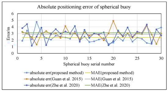
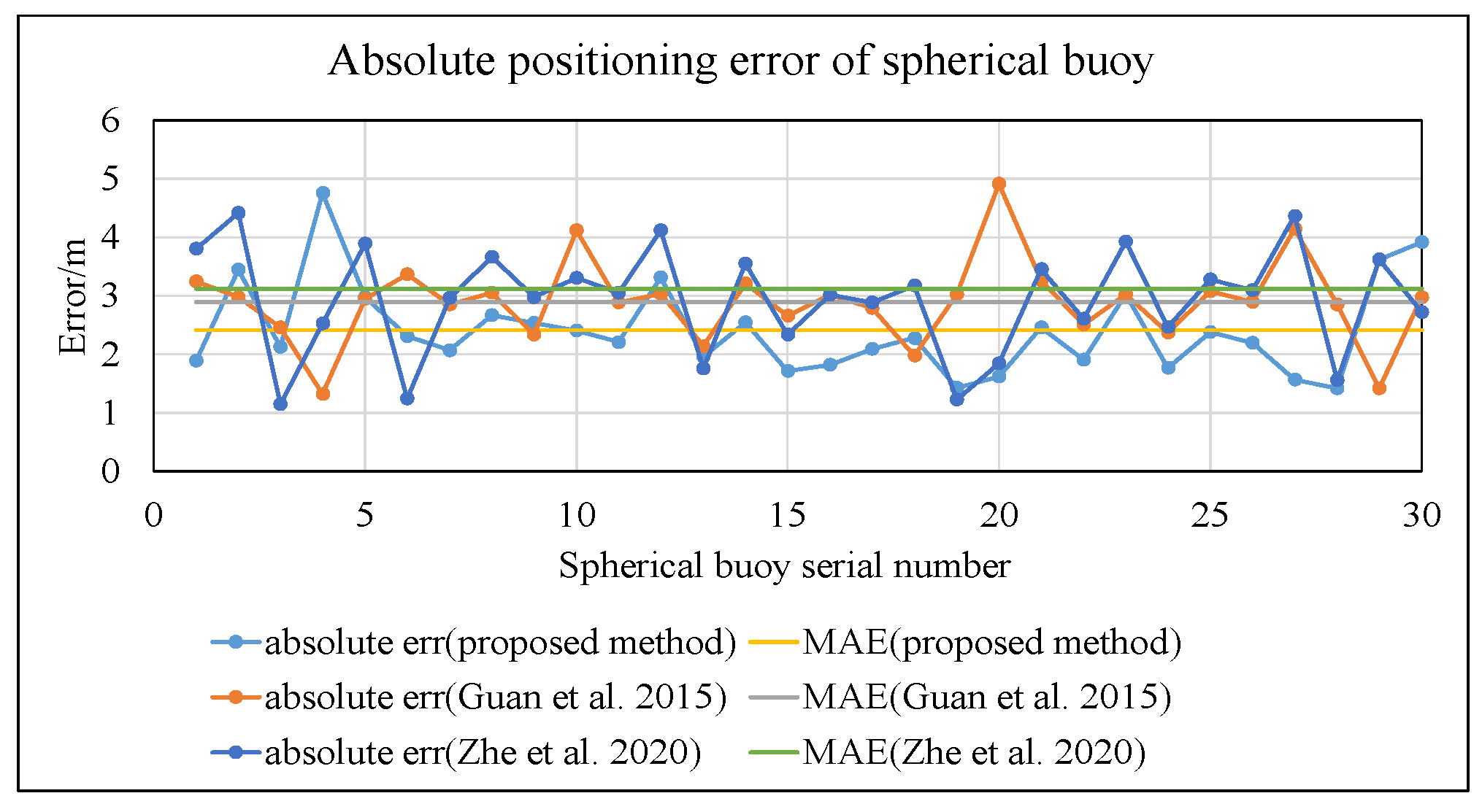
Figure 21.
Comparison chart of positioning results under low illumination, reflection, and water obstruction conditions (proposed method vs. Guan et al. [19] and Zhe et al. [40]).
As shown in Figure 21, the mean absolute error of the spherical buoy positions calculated using the method proposed in this paper is 2.42 m. This represents a reduction of 16.3% compared to the method in reference [19] (2.89 m) and a reduction of 22.4% compared to the method in reference [40] (3.12 m).
- (3)
- Low Water Transparency, Reflections, and Water Obstruction
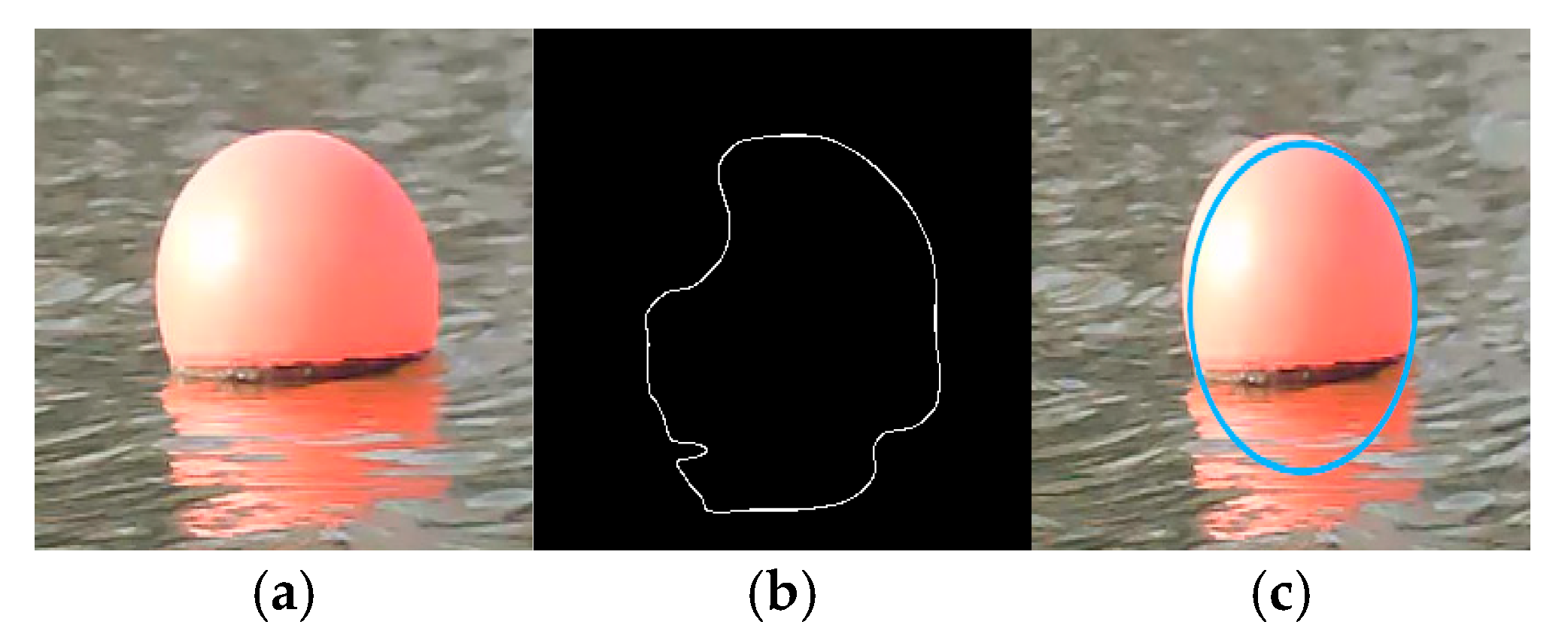
Figure 22a shows an image captured in a scenario with low water transparency, where reflections and obstructions exist. After preprocessing, the result is shown in Figure 22b, and the final contour reconstruction effect after applying the proposed ellipse fitting algorithm is shown in Figure 22c. The detection results demonstrate that the algorithm can effectively fit the complete contour of the spherical buoy in environments with low water transparency, reflections, and water obstructions.
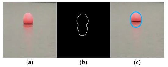
Figure 22.
Experimental environment: low water transparency, reflections, and water obstruction (red markers indicate spherical buoy, while blue contours represent fitted ellipse). (a) Original image. (b) Preprocessed image. (c) Ellipse fitting result.
In this environment, the comparison of absolute errors among the three methods is shown in Figure 23.
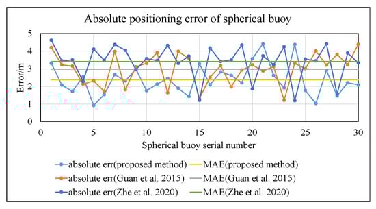
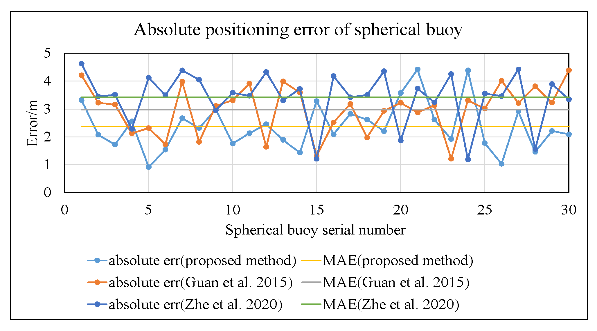
Figure 23.
Comparison chart of positioning results under conditions of low water transparency, reflection, and water obstruction (proposed method vs. Guan et al. [19] and Zhe et al. [40]).
As shown in Figure 23, the mean absolute error of the spherical buoy positions calculated using the method proposed in this study is 2.37 m. This represents a reduction of 20.5% compared to the method in reference [19] (2.98 m) and a reduction of 30.5% compared to the method in reference [40] (3.41 m).
- (4)
- Comparison of Positioning Results Before and After Correction
To quantitatively analyze the impact of lens distortion on the positioning accuracy of the camera used in this study, we performed lens distortion correction on images collected under conditions of strong illumination, reflections, and water occlusions. We then applied the positioning algorithm proposed in this paper to both the original and corrected images for location calculations. The images before and after distortion correction are shown in Figure 24a,b, respectively, while the positioning results before and after distortion correction are presented in Figure 25.
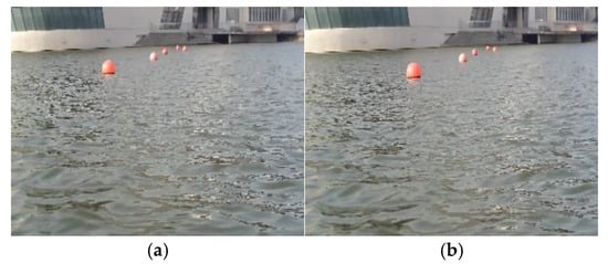
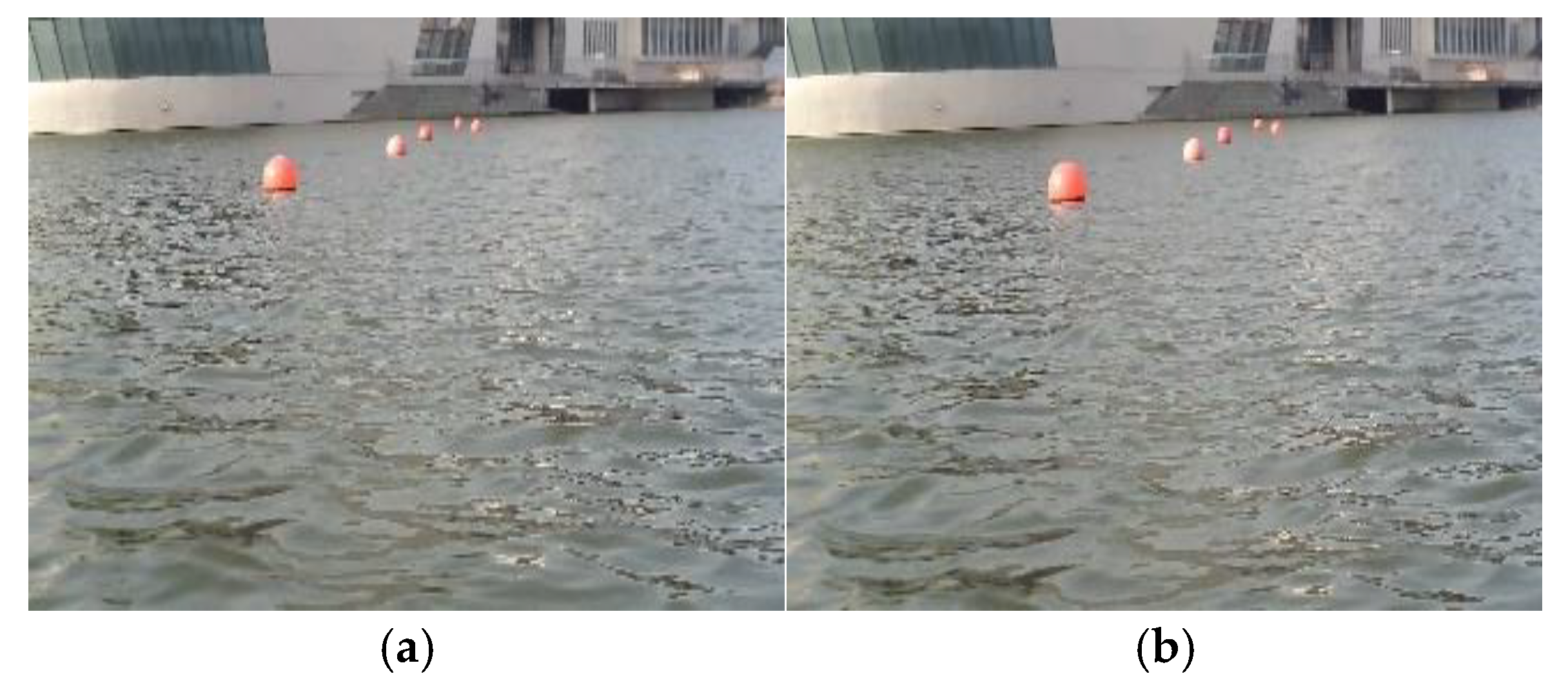
Figure 24.
Image comparison before and after correction. (a) Original image. (b) Corrected image.
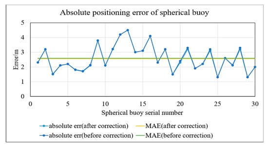
Figure 25.
Comparison of positioning results before and after correction.
From Figure 24a,b, it can be observed that the distortion phenomenon in the uncorrected image is not pronounced, resulting in no significant difference between the images before and after correction. According to the experimental results shown in Figure 25, the mean absolute error for the spherical buoy’s position before correction was 2.58 m, while after correction it was 2.57 m, with a difference of only 0.01 m between the two. This outcome indicates that the impact of the camera’s distortion on positioning accuracy is negligible.
In summary, the method proposed in this paper can stably detect spherical buoys and accurately reconstruct their contours under various complex environments, including high illumination, low illumination, low water transparency, water surface reflections, and partial occlusions. The experiments demonstrate that the impact of lens distortion on the positioning accuracy can be neglected. The coordinates obtained using the positioning algorithm proposed in this paper have an average absolute error of less than 2.57 m. Moreover, the algorithm achieves a processing speed of 109 milliseconds per frame, meeting both the requirements for positioning accuracy and real-time processing, thereby validating the practicality of the proposed method.
6. Conclusions
To address the issues of incomplete contours and weakened edge features of spherical buoys on the water surface due to water obstruction and strong illumination, this paper proposes a monocular vision-based localization method using elliptical fitting. This approach fits an ellipse to the target’s edges, leveraging prior knowledge of the spherical buoy’s radius to establish a monocular vision-based ranging model. It integrates the USV’s position from satellite observation in the scene to estimate the coordinates of each spherical buoy in the geodetic coordinate system. Additionally, to address the problem of pseudo-edge points introduced by water reflections affecting the performance of elliptical fitting, this paper presents a method based on grayscale feature analysis and RANSAC multiple outlier rejection for elliptical fitting, effectively filtering out pseudo-edge points to obtain accurate elliptical parameters. Simulation and onboard experiment results demonstrate that this method can accurately obtain the coordinates of spherical buoys in the geodetic coordinate system under disturbances such as water reflections, varying illumination, and water obstruction, with precision comparable to general satellite positioning. This verifies the effectiveness and practicality of the method, meeting the requirements for real-time applications. One limitation of this paper is the difficulty in effectively detecting the edges of spherical buoys under extremely low-light conditions. Therefore, designing algorithms for detecting spherical buoy edges in extremely low-light conditions will be a key focus of our future research.
Author Contributions
Conceptualization, J.W.; methodology, S.W.; software, S.W.; validation, S.W.; formal analysis, S.W.; investigation, S.W.; resources, J.W., X.Z. (Xianqiang Zeng) and G.W.; data curation, S.W.; writing—original draft preparation, S.W.; writing—review and editing, S.W., J.W. and X.Z. (Xiang Zheng); visualization, S.W.; supervision, J.W. and X.Z. (Xiang Zheng); project administration, J.W.; funding acquisition, G.W. All authors have read and agreed to the published version of the manuscript.
Funding
This study was supported by the National Natural Science Foundation of China, grant number 52271322.
Institutional Review Board Statement
Not applicable.
Informed Consent Statement
Not applicable.
Data Availability Statement
The original contributions presented in this study are included in this article. Further inquiries can be directed to the corresponding author.
Acknowledgments
The authors thank the anonymous reviewers for suggesting valuable improvements for this paper.
Conflicts of Interest
Author Xianqiang Zeng was employed by the company Shanghai Auto Subsea Vehicles Inc. The remaining authors declare that the research was conducted in the absence of any commercial or financial relationships that could be construed as a potential conflict of interest.
References
- Shin, S.S.; Park, S.D. Application of spherical-rod float image velocimetry for evaluating high flow rate in mountain rivers. Flow Meas. Instrum. 2021, 78, 101906. [Google Scholar] [CrossRef]
- Chen, Y.; Zhu, S.; Zhang, W.; Zhu, Z.; Bao, M. The model of tracing drift targets and its application in the South China Sea. Acta Oceanol. Sin. 2022, 41, 109–118. [Google Scholar] [CrossRef]
- Holland, D.; Landaeta, E.; Montagnoli, C.; Ayars, T.; Barnes, J.; Barthelemy, K.; Brown, R.; Delp, G.; Garnier, T.; Halleran, J. Design of the Minion Research Platform for the 2022 Maritime RobotX Challenge. Nav. Eng. J. 2024, 136, 125–137. [Google Scholar]
- Bowes, J.; Colby, I.; Thomas, B.; Hooper, T.; Zhao, S.; Ye, J.; Jenkins, A. Designing the RoboSeals’ RobotX 2022 Challenge. Available online: https://robonation.org/app/uploads/sites/2/2022/10/RX22_TDR_University-of-South-Australia.pdf (accessed on 5 January 2025).
- Aisyiyaturrosyadah, A.P.; Moko, D.; Anjarwati, F.; Putra, G.; Aulia, G.; Haqqani, G.; Rahman, I.; Rohmah, I.S.; Wardhana, M.; Alghifari, M. Roboboat 2024: Technical Design Report. 2024. Available online: https://robonation.org/app/uploads/sites/3/2023/12/TDR_Universitas-Sebelas-Maret_RB2024.pdf (accessed on 6 January 2025).
- Rusiecki, I.; Ujazdowski, T.; Wilk, J.; Sobolewski, P.; Pyskovatskyi, S.; Skierkowski, M.; Lisowski, T.; Sieklicki, W. Software Architecture Design of ASV Rybitwa: Development of an Autonomous Surface Vehicle for Dynamic Navigation and Task Execution. In Proceedings of the Journal of Physics: Conference Series, Trondheim, Norway, 29–30 October 2024; p. 012031. [Google Scholar]
- Woo, J.; Lee, J.; Kim, N. Obstacle avoidance and target search of an autonomous surface vehicle for 2016 maritime robotx challenge. In Proceedings of the 2017 IEEE Underwater Technology (UT), Tokyo, Japan, 21–24 February 2017; pp. 1–5. [Google Scholar]
- Stanislas, L.; Moyle, K.; Corser, E.; Ha, T.; Dyson, R.; Lamont, R.; Dunbabin, M. Bruce: A system-of-systems solution to the 2018 Maritime RobotX Challenge. 2018. Available online: https://robonation.org/app/uploads/sites/2/2019/09/QUT_RX18_Paper.pdf (accessed on 6 January 2025).
- Hou, C.; Zhang, X.; Tang, Y.; Zhuang, J.; Tan, Z.; Huang, H.; Chen, W.; Wei, S.; He, Y.; Luo, S. Detection and localization of citrus fruit based on improved You Only Look Once v5s and binocular vision in the orchard. Front. Plant Sci. 2022, 13, 972445. [Google Scholar]
- Yang, B.; Yang, B.; Liu, J. Research on adjustable baseline binocular vision measurement system. Int. J. Front. Eng. Technol. 2022, 4, 30–34. [Google Scholar]
- Arampatzakis, V.; Pavlidis, G.; Mitianoudis, N.; Papamarkos, N. Monocular depth estimation: A thorough review. IEEE Trans. Pattern Anal. Mach. Intell. 2023, 46, 2396–2414. [Google Scholar]
- Dong, X.; Garratt, M.A.; Anavatti, S.G.; Abbass, H.A. Towards real-time monocular depth estimation for robotics: A survey. IEEE Trans. Intell. Transp. Syst. 2022, 23, 16940–16961. [Google Scholar]
- Vyas, P.; Saxena, C.; Badapanda, A.; Goswami, A. Outdoor monocular depth estimation: A research review. arXiv 2022, arXiv:2205.01399. [Google Scholar]
- Penne, R.; Ribbens, B.; Roios, P. An exact robust method to localize a known sphere by means of one image. Int. J. Comput. Vis. 2019, 127, 1012–1024. [Google Scholar] [CrossRef]
- Van Zandycke, G.; De Vleeschouwer, C. 3D ball localization from a single calibrated image. In Proceedings of the IEEE/CVF Conference on Computer Vision and Pattern Recognition, New Orleans, LA, USA, 18–24 June 2022; pp. 3472–3480. [Google Scholar]
- Hajder, L.; Toth, T.; Pusztai, Z. Automatic estimation of sphere centers from images of calibrated cameras. arXiv 2020, arXiv:2002.10217. [Google Scholar]
- Zhao, Q.; Li, Q.; Li, C.; He, Y.; Zeng, R. A Monocular Ball Localization Method for Automatic Hitting Robots. In Proceedings of the 2023 IEEE International Conference on Unmanned Systems (ICUS), Hefei, China, 13–15 October 2023; pp. 1–6. [Google Scholar]
- Budiharto, W.; Kanigoro, B.; Noviantri, V. Ball distance estimation and tracking system of humanoid soccer robot. In Proceedings of the Information and Communication Technology: Second IFIP TC5/8 International Conference, ICT-EurAsia 2014, Bali, Indonesia, 14–17 April 2014; Proceedings 2. pp. 170–178. [Google Scholar]
- Guan, J.; Deboeverie, F.; Slembrouck, M.; Van Haerenborgh, D.; Van Cauwelaert, D.; Veelaert, P.; Philips, W. Extrinsic calibration of camera networks using a sphere. Sensors 2015, 15, 18985–19005. [Google Scholar] [CrossRef] [PubMed]
- Liu, T.; Pang, B.; Zhang, L.; Yang, W.; Sun, X. Sea surface object detection algorithm based on YOLO v4 fused with reverse depthwise separable convolution (RDSC) for USV. J. Mar. Sci. Eng. 2021, 9, 753. [Google Scholar] [CrossRef]
- Zhao, J.; McMillan, C.; Xue, B.; Vennell, R.; Zhang, M. Buoy detection under extreme low-light illumination for intelligent mussel farming. In Proceedings of the 2023 38th International Conference on Image and Vision Computing New Zealand (IVCNZ), Palmerston North, New Zealand, 29–30 November 2023; pp. 1–6. [Google Scholar]
- Kang, B.-S.; Jung, C.-H. Detecting maritime obstacles using camera images. J. Mar. Sci. Eng. 2022, 10, 1528. [Google Scholar] [CrossRef]
- Zhang, L.; Zhang, Y.; Zhang, Z.; Shen, J.; Wang, H. Real-time water surface object detection based on improved faster R-CNN. Sensors 2019, 19, 3523. [Google Scholar] [CrossRef] [PubMed]
- Zhang, L.; Wei, Y.; Wang, H.; Shao, Y.; Shen, J. Real-time detection of river surface floating object based on improved refinedet. IEEE Access 2021, 9, 81147–81160. [Google Scholar]
- Cao, Y.-J.; Lin, C.; Li, Y.-J. Learning crisp boundaries using deep refinement network and adaptive weighting loss. IEEE Trans. Multimed. 2020, 23, 761–771. [Google Scholar]
- Huan, L.; Xue, N.; Zheng, X.; He, W.; Gong, J.; Xia, G.-S. Unmixing convolutional features for crisp edge detection. IEEE Trans. Pattern Anal. Mach. Intell. 2021, 44, 6602–6609. [Google Scholar] [CrossRef] [PubMed]
- Lin, C.; Cui, L.; Li, F.; Cao, Y. Lateral refinement network for contour detection. Neurocomputing 2020, 409, 361–371. [Google Scholar]
- Liu, Y.; Cheng, M.-M.; Hu, X.; Wang, K.; Bai, X. Richer convolutional features for edge detection. In Proceedings of the IEEE conference on computer vision and pattern recognition, Honolulu, HI, USA, 21–26 July 2017; pp. 3000–3009. [Google Scholar]
- Khan, S.H.; Bennamoun, M.; Sohel, F.; Togneri, R. Automatic feature learning for robust shadow detection. In Proceedings of the 2014 IEEE conference on computer vision and pattern recognition, Columbus, OH, USA, 23–28 June 2014; pp. 1939–1946. [Google Scholar]
- Zheng, W.; Teng, X. Image Shadow Removal Based on Residual Neural Network. In Proceedings of the 2018 International Conference on Security, Pattern Analysis, and Cybernetics (SPAC), Jinan, China, 14–17 December 2018; pp. 429–434. [Google Scholar]
- Aqthobilrobbany, A.; Handayani, A.N.; Lestari, D.; Asmara, R.A.; Fukuda, O. HSV Based Robot Boat Navigation System. In Proceedings of the 2020 International Conference on Computer Engineering, Network, and Intelligent Multimedia (CENIM), Surabaya, Indonesia, 17–18 November 2020; pp. 269–273. [Google Scholar]
- Tran, L.; Selfridge, J.; Hou, G.; Li, J. Marine Buoy Detection Using Circular Hough Transform. In Proceedings of the AUVSI Unmanned Systems North America Conference 2011, Washington, DC, USA, 16–19 August 2011. [Google Scholar]
- Shafiabadi, M.; Kamkar-Rouhani, A.; Riabi, S.R.G.; Kahoo, A.R.; Tokhmechi, B. Identification of reservoir fractures on FMI image logs using Canny and Sobel edge detection algorithms. Oil Gas Sci. Technol. –Rev. D’ifp Energ. Nouv. 2021, 76, 10. [Google Scholar]
- Isar, A.; Nafornita, C.; Magu, G. Hyperanalytic wavelet-based robust edge detection. Remote Sens. 2021, 13, 2888. [Google Scholar] [CrossRef]
- Dwivedi, D.; Chamoli, A. Source edge detection of potential field data using wavelet decomposition. Pure Appl. Geophys. 2021, 178, 919–938. [Google Scholar]
- Li, Y.; Zhou, J.; Huang, F.; Liu, L. Sub-pixel extraction of laser stripe center using an improved gray-gravity method. Sensors 2017, 17, 814. [Google Scholar] [CrossRef] [PubMed]
- Chen, Y.; Li, Y.; Zhao, Y. Sub-pixel detection algorithm based on cubic B-spline curve and multi-scale adaptive wavelet transform. Optik 2016, 127, 11–14. [Google Scholar] [CrossRef]
- İmre, E.; Hilton, A. Order statistics of RANSAC and their practical application. Int. J. Comput. Vis. 2015, 111, 276–297. [Google Scholar]
- Tang, Y.; Srihari, S.N. Ellipse detection using sampling constraints. In Proceedings of the 2011 18th IEEE International Conference on Image Processing, Brussels, Belgium, 11–14 September 2011; pp. 1045–1048. [Google Scholar]
- Zhe, T.; Huang, L.; Wu, Q.; Zhang, J.; Pei, C.; Li, L. Inter-vehicle distance estimation method based on monocular vision using 3D detection. IEEE Trans. Veh. Technol. 2020, 69, 4907–4919. [Google Scholar]


Disclaimer/Publisher’s Note: The statements, opinions and data contained in all publications are solely those of the individual author(s) and contributor(s) and not of MDPI and/or the editor(s). MDPI and/or the editor(s) disclaim responsibility for any injury to people or property resulting from any ideas, methods, instructions or products referred to in the content. |
© 2025 by the authors. Licensee MDPI, Basel, Switzerland. This article is an open access article distributed under the terms and conditions of the Creative Commons Attribution (CC BY) license (https://creativecommons.org/licenses/by/4.0/).