Co-Optimization of the Hardware Configuration and Energy Management Parameters of Ship Hybrid Power Systems Based on the Hybrid Ivy-SA Algorithm

Abstract

A ship’s diesel–electric hybrid power system is complex, with hardware configuration and energy management parameters being crucial to its economic performance. However, existing optimization methods typically involve designing and optimizing the hardware configuration on the basis of typical operating conditions, followed by the design and optimization of the energy management parameters, which makes it difficult to achieve optimal system performance. Moreover, when co-optimizing hardware configurations and energy management parameters, the parameter relationships and complex constraints often lead conventional optimization algorithms to converge slowly and become trapped in local optima. To address this issue, a hybrid Ivy-SA algorithm is developed for the co-optimization of both the hardware configuration and energy management parameters. First, the main engine and hybrid ship models are established on the basis of the hardware configuration, and the accuracy of the models is validated. An energy management strategy based on the equivalent fuel consumption minimization strategy (ECMS) is then formulated, and energy management parameters are designed. A sensitivity analysis is conducted on the basis of both the hardware configuration and energy management parameters to evaluate their impacts under various conditions, enabling the selection of key optimization parameters, such as diesel engine parameters, battery configuration, and charge/discharge factors. The Ivy-SA algorithm, which integrates the advantages of both the Ivy algorithm (IVYA) and the simulated annealing algorithm (SA), is developed for the co-optimization. The algorithm is tested with the CEC2017 benchmark functions and outperforms 11 other algorithms. Furthermore, when the top five performing algorithms are applied for the co-optimization, the results show that the Ivy-SA algorithm outperforms the other four algorithms with a 14.49% increase in economic efficiency and successfully escapes local optima.

1. Introduction

Although diesel engines exhibit advantages such as high power density, few intermediate components, and high reliability, they often fail to operate within an efficient range when ships are under light loads. This results in decreased fuel efficiency and increased emissions. With the rapid advancements in energy storage, charging, and power electronics technologies, the use of novel hybrid power systems in ship designs has become a practical option to improve energy utilization [1]. An increasing number of ships are adopting multiple forms of energy, including various fuels (such as bio-LNG, bio-methanol, and ammonia), power batteries, and fuel cells. A single fuel cannot dominate the future [2,3]. Diesel–electric hybrid ships can switch between multiple operating modes on the basis of complex and variable working conditions, maintaining high fuel economy while reducing mechanical vibrations. They offer significant advantages in increasing energy efficiency, reducing emissions, and increasing operational stability [4]. Therefore, diesel–electric hybrid ships have become a key research focus in this field [5].

1.1. Hardware Configuration of Ship Hybrid Power Systems

Improving the performance of ship hybrid propulsion systems involves optimizing both the hardware configuration of the power system and the energy management strategies. The key elements of the diesel–electric hybrid system are the diesel engine and the power battery, with their performance and configuration being crucial to the system’s overall efficiency. Tadros et al. [6] minimized engine fuel consumption by optimizing adjustable parameters such as the turbocharger speed, injection timing, intake valve timing, and fuel injection amount. Liu et al. [7] improved the thermal efficiency and reduced NOx emissions by optimizing the injection timing, duration, and quantity. Furthermore, Chen et al. [8] selected parameters such as the injection timing, intake cam phase, intake valve, intake temperature, and pressure to optimize brake-specific fuel consumption, combustion noise, and NOx emissions under different load conditions. In addition, Li et al. [9] designed a capacity optimization method that involves joint optimization of the allocated power and capacity, reducing the total lifecycle cost of the hybrid power system. Barrera-Cardenas et al. [10] investigated free design parameters and analyzed the tradeoffs among different performance metrics, determining the optimal size of a ship’s battery energy storage system (BESS). Balci et al. [11] employed Interpretive Structural Modeling (ISM) and Cross-Impact Matrix Multiplication Applied to Classification (MICMAC) to reveal the relationship between success factors of the industry-wide adoption of green ammonia. This method also facilitates the analysis and application of ship hybrid power systems.

1.2. Energy Management Strategies for Hybrid Ships

The formulation of the energy management strategy determines the coordination among various components of the power system and directly influences the performance of hybrid power systems. Visser et al. [12] proposed an energy management strategy based on model predictive control (MPC), which, when applied to naval vessels, reduced fuel consumption by 3.5%. In addition, Liu et al. [13] introduced an energy efficiency optimization strategy for hybrid ships based on predicting the operational conditions. By forecasting factors such as the wind speed and current velocity using time series analysis, the challenges associated with future operational conditions can be addressed with this strategy. Moreover, Wang et al. [14] employed an improved K-means++ algorithm to divide ship routes and developed an energy management strategy for diesel–electric hybrid ships based on the deep deterministic policy gradient (DDPG) algorithm, optimizing the operating range of the diesel engine. Gao et al. [15] proposed an energy optimization strategy based on predicted load power, considering the economic performance, emissions, and endurance of hybrid ships, leading to improvements in fuel economy and endurance.

1.3. Optimization Algorithms for Hybrid Ships

Ship hybrid power systems are complex, and to achieve optimal performance, numerous optimization algorithms, such as particle swarm optimization (PSO), genetic algorithms (GAs), gray wolf optimization (GWO), and MOEA/D, have been introduced. In terms of the hardware configuration, the diesel engine parameters directly impact fuel consumption and emissions, whereas the configuration of the lithium batteries significantly affects the cost, lifespan, and energy efficiency of the system. With respect to the energy management strategies, energy management parameters determine the power allocation between the engine and the battery. Tjandra et al. [16] proposed an optimization technique for the battery storage systems of hybrid ships that combines the multi-objective particle swarm optimization (MOPSO) algorithm and the nondominated sorting GA II (NSGA-II). Xiang et al. [17] proposed an improved ant colony optimization (ACO) algorithm to optimize the equivalence factor of the equivalent fuel consumption minimization strategy (ECMS) considering mode switching, reducing the deviation between the final state of charge (SOC) value and the target value. Chen et al. [18] applied a hybrid algorithm that combines a chaotic optimization algorithm with the GWO algorithm to address nonlinear optimization issues in predictive control strategies, further optimizing the performance of the energy management system. Shang et al. [19] used the GWO algorithm to optimize the membership functions of fuzzy control inputs and outputs, improving the performance of the fuzzy control strategy.

1.4. Summary

Previous studies indicate that the optimization of hybrid power systems typically involves the following two main strategies: optimizing the energy management strategies by adjusting the energy management parameters of the system while keeping the hardware configuration fixed, or optimizing the hardware configuration, such as the battery and diesel engine parameters, while applying a predefined control strategy. However, regardless of the energy management strategy, the energy management parameters and hardware configuration of the hybrid power system are interdependent. Thus, optimizing one aspect in isolation cannot guarantee optimal performance for the overall system. Furthermore, the effectiveness of the optimization process is largely determined by the ability of the optimization algorithm to search for the optimal solution and its stability. In existing optimization algorithms, hardware configurations and energy management parameters are optimized separately. However, these methods have significant limitations in optimizing both the hardware configuration and energy management parameters simultaneously. In highly coupled systems, these algorithms often become trapped in local optima. As the model becomes more complex and detailed, the computational complexity increases exponentially, leading to inefficiency and long system response times. Additionally, existing algorithms have limited abilities to handle uncertainties and fuzziness in the system, causing substantial deviations in optimization solutions with small disturbances. Therefore, the development of an optimization algorithm capable of simultaneously optimizing both the hardware configuration and energy management parameters is the central focus of this study.

1.5. The Main Research Content of This Paper

This study focuses on a hybrid diesel–electric propulsion ship and develops the Ivy-SA algorithm. The Ivy-SA algorithm effectively combines the SA algorithm’s ability to escape local optima with the rapid convergence characteristics of the IVYA. By applying the PSO, GWO, IVYA, SA, and Ivy-SA algorithms, the hardware parameters and energy management parameters of the hybrid power system are co-optimized, improving the system’s economic efficiency. The results show that the Ivy-SA algorithm achieves better optimization performance compared to the other four algorithms. The main contributions of the paper are as follows:

• The main engine model and hybrid ship model are established on the basis of the hardware configuration, and the accuracy of the models is validated.
• To meet the real-time response requirements of the system, an ECMS-based energy management strategy is formulated, and energy management parameters are set.
• A sensitivity analysis is conducted based on the hardware configuration and energy management parameters to determine the optimization parameters.
• The Ivy-SA algorithm is developed and tested with the CEC2017 benchmark functions, concurrently optimizing the hardware configuration and the energy management parameters of the hybrid power system.

2. Hybrid Power System Modeling

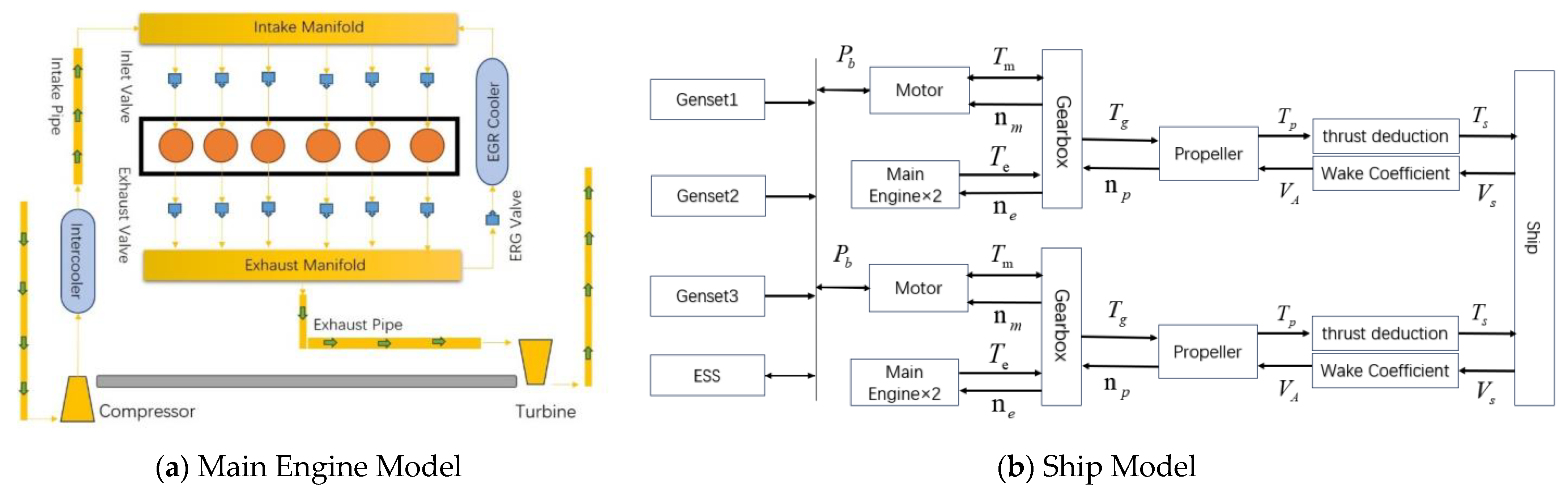
2.1. Diesel Engine Model

The operation of a diesel engine is a comprehensive thermodynamic process that involves multiple disciplines, including fuel combustion, heat and mass transfer, and various physical and chemical phenomena. Depending on the research objectives and application scenarios, different simplifications of the thermodynamic process of the diesel engine are necessary. This approach not only enables the prediction of the engine’s basic performance but also facilitates this study and comparison of various parameter configurations, thereby optimizing both the structural and operating parameters of internal combustion engines. Consequently, it greatly reduces experimental workload, shortens research and development cycles, and saves human resources and development costs. Diesel engine simulations are primarily based on the theories of combustion exothermicity, heat transfer, fluid dynamics, and other related disciplines. These simulations employ advanced numerical methods from higher mathematics and integrate extensive experimental data while fully accounting for factors such as combustion chamber structure, fuel injection, combustion models, intake/exhaust flow boosting methods, and intercooling configurations [20].

(1)

In-Cylinder Thermodynamic Calculation

During the process of establishing the diesel engine cylinder model, under the assumptions of zero-dimensional conditions and quasi-steady flow, neglecting the kinetic energy of the gas inflow and outflow, and applying the first law of thermodynamics, the law of mass conservation, the ideal gas equation of state, and appropriate transformations, a general set of equations for calculating the working process of an internal combustion engine can be derived [21].

The rate of temperature change for the working medium in the cylinder is expressed as follows:

$${\displaystyle \frac{dT}{d\phi }}={\displaystyle \frac{1}{m{c}_v}}\left({\displaystyle \frac{d{Q}_B}{d\phi }}+{\displaystyle \frac{d{Q}_W}{d\phi }}-p{\displaystyle \frac{dV}{d\phi }}+h_s{\displaystyle \frac{d{m}_s}{d\phi }}+h_e{\displaystyle \frac{d{m}_e}{d\phi }}-u{\displaystyle \frac{dm}{d\phi }}-{\displaystyle \frac{\mathit{\partial }u}{\mathit{\partial }\lambda }}{\displaystyle \frac{d\lambda }{d\phi }}\right)$$

(1)

where $u$ represents the specific internal energy, $p$ represents the pressure of the working medium in the cylinder, $V$ represents the working volume of the cylinder, $Q_B$ represents the heat released by fuel combustion in the cylinder, $Q_W$ represents the heat transferred through the cylinder walls, $m_s$ represents the mass of air entering the cylinder, $m_e$ represents the mass of exhaust gases leaving the cylinder, and $h_s,h_e$ represent the specific enthalpies of the working medium at the intake and exhaust valves, respectively.

The instantaneous working volume of the cylinder is determined by the variation in piston displacement, which can be expressed as follows:

$$V\left(\phi \right)={\displaystyle \frac{V_h}{2}}\left({\displaystyle \frac{2}{\epsilon -1}}+1-\cos \phi +{\displaystyle \frac{1}{{\lambda }_s}}\left(1-\sqrt{1-{\lambda }_s^2{\sin }^2\phi }\right)\right)$$

(2)

The rate of change of the instantaneous working volume within the cylinder is given by the following equation:

$${\displaystyle \frac{dV}{d\phi }}={\displaystyle \frac{V_h}{2}}\left(\sin \phi +{\lambda }_s{\displaystyle \frac{\sin \phi \cos \phi }{\sqrt{1-{\lambda }_s^2{\sin }^2\phi }}}\right)$$

(3)

where $\epsilon$ represents the compression ratio; $\phi$ represents the crankshaft angle, measured from the top dead center (TDC), where $\phi =0$; and ${\lambda }_s$ represents the connecting rod to crank radius ratio.

The heat transfer through the cylinder wall of the diesel engine includes the heat losses through the cylinder head, the inner surface of the cylinder liner, and the piston crown. The calculation for the cylinder wall heat transfer is given by the following equation:

$${\displaystyle \frac{d{Q}_W}{d\phi }}=\sum _{i=1}^3{\displaystyle \frac{d{Q}_{Wi}}{d\phi }}={\displaystyle \frac{1}{\omega }}\sum _{i=1}^3{\alpha }_g{A}_i\left(T-T_{wi}\right)$$

(4)

where $\omega$ represents the angular velocity, ${\alpha }_g$ represents the instantaneous average heat transfer coefficient, $A$ represents the heat transfer area, and $T_{wi}$ represents the average temperature of the wall.

The variations in temperature and pressure of the working medium within the cylinder, as functions of the crankshaft angle, are primarily determined by the heat release rate of fuel combustion. These variations significantly influence the diesel engine’s efficiency and emissions. The instantaneous heat release rate during in-cylinder combustion is given by the following equation:

$${\displaystyle \frac{d{Q}_B}{d\phi }}=6.908 \times {\displaystyle \frac{{\eta }_u\times m_{B0}\times H_u}{\Delta \phi }}\left(m+1\right){\left({\displaystyle \frac{\phi -{\phi }_{VB}}{\Delta \phi }}\right)}^{m+1}\times \exp \left[-6.908{\left({\displaystyle \frac{\phi -{\phi }_{VB}}{\Delta \phi }}\right)}^{m+1}\right]$$

(5)

where ${\eta }_u$ represents the combustion efficiency, $m_{B0}$ represents the mass of fuel supplied per cycle, $H_u$ represents the lower heating value of the fuel, ${\phi }_{VB}$ represents the start of combustion, $\Delta \phi$ represents the combustion duration, and $m$ represents the combustion quality index.

(2)

Intake and Exhaust Mass Flow Rate

During the operation of an internal combustion engine, the inflow and outflow of gases through the intake and exhaust valves can be regarded as quasi-steady flow. That is, when the calculated time interval is sufficiently small, the gas flow process within this interval can be considered stable [22].

The intake flow at the intake valve of an internal combustion engine is generally a subcritical sonic flow process, and its mass flow rate variation is given by the following equation:

$${\displaystyle \frac{d{m}_s}{d\phi }}={\displaystyle \frac{1}{6n}}\times F_s\times {\displaystyle \frac{P_s}{\sqrt{R_s\times T_s}}}\times \sqrt{{\displaystyle \frac{2k_s}{k_s-1}}\left[{\left({\displaystyle \frac{P}{P_s}}\right)}^{{\displaystyle \frac{2}{k_s}}}-{\left({\displaystyle \frac{P}{P_s}}\right)}^{{\displaystyle \frac{k_s+1}{k_s}}}\right]}$$

(6)

where $n$ represents the engine speed, $F_s$ represents the instantaneous geometric flow area, $P_s$ represents the working medium pressure upstream, $T_s$ represents the working medium temperature upstream, $R_s$ represents the specific gas constant of the working medium upstream, $k_s$ represents the adiabatic index of the working medium upstream, and $P$ represents the working medium pressure downstream.

At the initial stage of exhaust valve opening, due to the significant pressure difference between the upstream (inside the cylinder) and downstream (exhaust port) of the exhaust valve, a supercritical sonic flow process may occur. Subsequently, as the pressure difference across the exhaust valve decreases, the flow transitions to a general subcritical flow regime.

When ${\displaystyle \frac{P_{\mathrm{ex}}}{P}}\le {\left({\displaystyle \frac{2}{k+1}}\right)}^{{\displaystyle \frac{k}{k-1}}}$, the mass flow rate variation is given by the following equation:

$${\displaystyle \frac{d{m}_e}{d\phi }}={\displaystyle \frac{1}{6n}}\times F_e\times {\displaystyle \frac{P}{\sqrt{R\times T}}}\times {\left({\displaystyle \frac{2}{k+1}}\right)}^{{\displaystyle \frac{k}{k-1}}}\times \sqrt{{\displaystyle \frac{2k}{k+1}}}$$

(7)

When ${\displaystyle \frac{P_{\mathrm{ex}}}{P}}>{\left({\displaystyle \frac{2}{k+1}}\right)}^{{\displaystyle \frac{k}{k-1}}}$, the mass flow rate variation is given by the following equation:

$${\displaystyle \frac{d{m}_e}{d\phi }}={\displaystyle \frac{1}{6n}}\times F_e\times {\displaystyle \frac{P}{\sqrt{R\times T}}}\times \sqrt{{\displaystyle \frac{2k}{k-1}}\left[{\left({\displaystyle \frac{P_{\mathrm{ex}}}{P}}\right)}^{{\displaystyle \frac{2}{k}}}-{\left({\displaystyle \frac{P_{\mathrm{ex}}}{P}}\right)}^{{\displaystyle \frac{k+1}{k}}}\right]}$$

(8)

where $F_e$ represents the instantaneous geometric flow area, $R$ represents the specific gas constant of the working fluid upstream, $k$ represents the adiabatic index of the working fluid upstream, and $P_{\mathrm{ex}}$ represents the working fluid pressure downstream.

(3)

Turbocharger

The internal combustion engine and the turbocharger operate in an interconnected manner by utilizing exhaust gas energy and fresh air supply. The turbocharger primarily consists of a compressor, an intermediate connecting shaft, and a turbine. The turbine harnesses the energy from the exhaust gases expelled by the engine to drive the compressor, which then supplies an adequate amount of fresh air to the engine.

The key parameters of the engine are shown in

Table 1. Main engine parameters.

Certain Type of 4-Stroke Diesel Engine	Parameter
Cylinder number	6
Cylinder arrangement	Inline
Engine type	4-stroke
Piston displacement	96.4 L/cyl
Engine speed	600 rpm
Engine output	7200 kW
Bore	460 mm
Stroke	580 mm
Mean piston speed	11.6 m/s

. On the basis of these parameters, an engine operation model was constructed, as illustrated in Figure 1a.

2.2. Ship Power System Model

This study focuses on a series–parallel hybrid-powered ro-pax vessel, which is a commercially operated ship traveling between Finland and Sweden, providing both passenger and cargo transportation services. The operating company of the vessel actively promotes sustainable development and complies with international environmental regulations. By optimizing and improving the vessel’s power system, the company aims to reduce fuel consumption and carbon emissions, meet energy efficiency and environmental sustainability goals, and simultaneously lower operational costs.

During a ship’s voyage [23], the control equation for the ship is as follows:

$${\displaystyle \frac{dv}{dt}}={\displaystyle \frac{1}{m+m_c}}\times (T+R_{sp}+R_A+F_{ext})$$

(9)

$$R_t=R_F+R_W=C_T \times A_W\times {\displaystyle \frac{1}{2}}\rho \times V_S^2$$

(10)

where ${\displaystyle \frac{dv}{dt}}$ represents the ship’s acceleration; $m$ and $m_c$ represent the masses of the ship and cargo, respectively; $T$ represents the thrust provided by the propeller; $R_{sp}$ represents the self-propelled resistance of the ship hull; $R_A$ represents the aerodynamic resistance; $F_{ext}$ represents the external force provided by any other mechanical connection; $R_F$ represents the friction resistance; $R_W$ represents the wave-making resistance; $C_T$ represents the total resistance coefficient; $A_W$ represents the wetted surface area; $\rho$ represents the water density; and $V_S$ represents the longitudinal velocity of the ship relative to the current.

During its rotation, the propeller absorbs the power transmitted through the shaft, generating thrust to propel the ship forward. The relative velocity of the propeller to the water and the advance ratio are given by the following equations:

$$V_A=V_S\times (1-\omega )$$

(11)

$$J={\displaystyle \frac{V_A}{n\times D}}$$

(12)

where $\omega$ represents the wake fraction and $n$ and $D$ are the propeller’s rotational speed and diameter, respectively.

For a controllable pitch propeller, the thrust coefficient $K_T$ and torque coefficient $K_Q$ are typically specified as functions of the advance ratio $J$ and the propeller pitch position $p$:

$$\left\{\begin{array}{c}{K}_T=f_{K_T}\left(J,p\right)\\ K_Q=f_{K_Q}\left(J,p\right)\end{array}\right.$$

(13)

The propeller thrust and torque are given by the following equation:

$$\left\{\begin{array}{c}T=K_T\times \rho \times n^2\times D^4\\ T=K_Q\times \rho \times n^2\times D^5\end{array}\right.$$

(14)

The motor’s characteristics are described by its rated parameters, and it can function as either a motor or a generator when needed.

The battery is modeled using an equivalent circuit model. The battery’s state of charge (SOC) is calculated by integrating the instantaneous current ($I_{OC}$) over time to determine the capacity change over the simulation duration. The instantaneous capacity is obtained by subtracting this capacity change from the initial capacity as follows [24]:

$$\left\{\begin{array}{c}C\left(t\right)=C_{Init}-{\int }_0^t{I}_{OC}dt\\ C_{Init}={SOC}_{Init}\times C_{Max}\\ SOC={\displaystyle \frac{C\left(t\right)}{C_{Max}}}\end{array}\right.$$

(15)

Based on the system parameters of each subsystem, the corresponding sub-models of the system are established. Then, according to the power and torque allocation requirements, each component is connected to form a complete hybrid power system, as shown in Figure 1b. The key parameters of each component in the hybrid power system are listed in

Table 2. Hybrid power system parameters.

Title	Parameter	Unit	Value
Main engine	Number	-	4
	Rated power	kW	7200
	Rated speed	r/min	600
GenSet	Number	-	3
	Rated power	kW	2610
Motor	Number	-	2
	Rated power	kW	2500
	Rated speed	r/min	675
Propeller	Type	-	CPP
	Diameter	m	5.4
Gearbox	ME reduction gear ratio	-	4.6
	Motor reduction gear ratio	-	2
Battery	Type	-	Ternary lithium battery
	Energy	kWh	4972

.

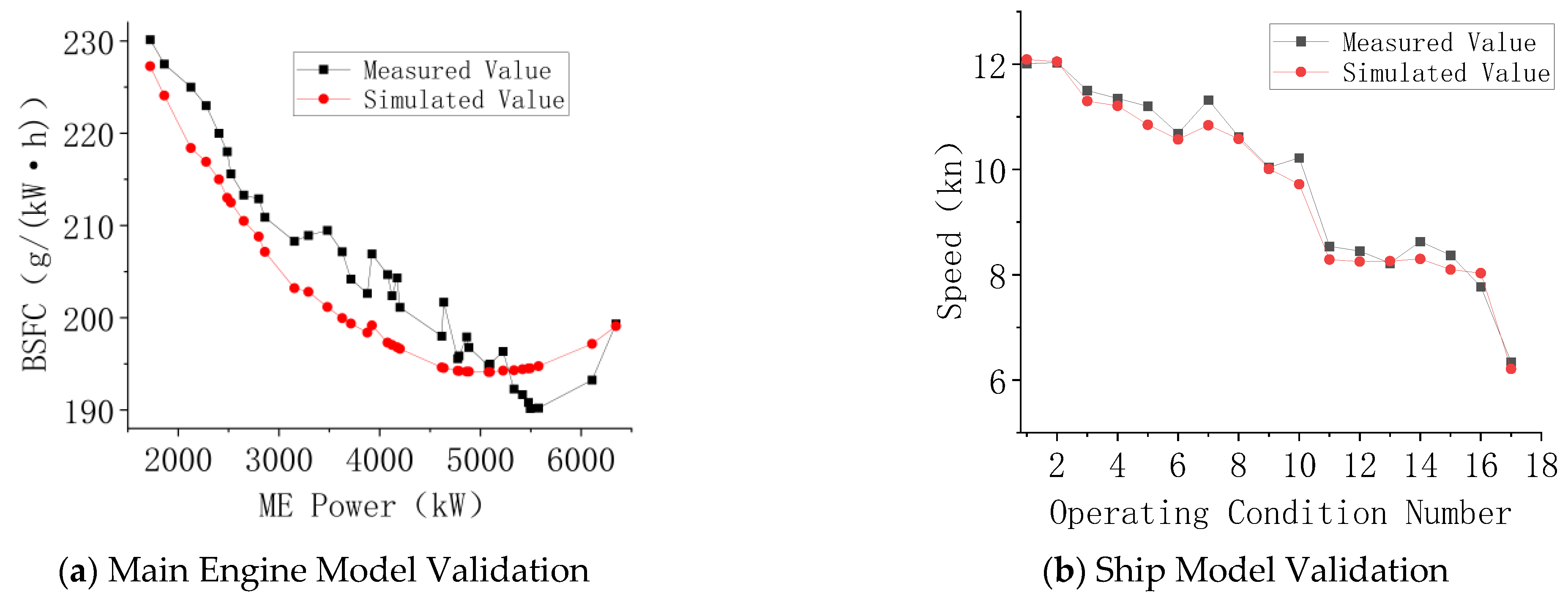
2.3. Model Validation

After the ship’s diesel engine model and power system model were established, the ship’s sea trial report was used for validation. First, the brake-specific fuel consumption (BSFC) of the diesel engine model was compared with that of a real diesel engine under various operating conditions, with a maximum relative error of 3.75%, as shown in Figure 2a. Then, under 17 actual operating conditions, the speed of the simulated ship was compared with the speed of an actual ship, with a maximum relative error of 3.84%, as shown in Figure 2b. The results indicate that the model accurately reflects the operational characteristics of the real system and meets the simulation requirements.

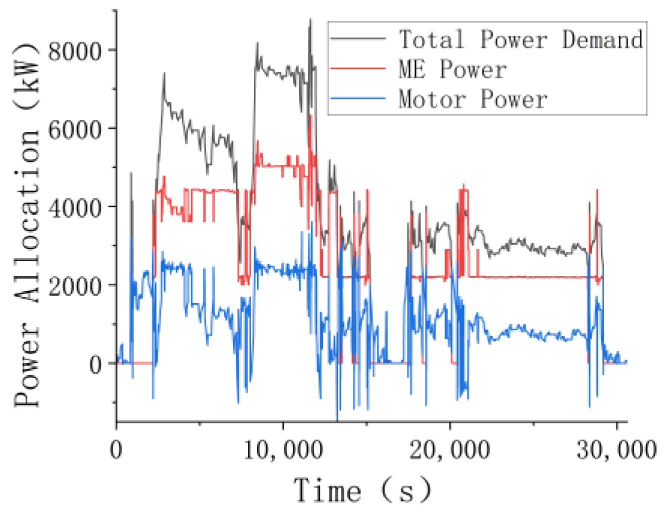
3. Energy Management Strategy

The ECMS is a classic energy management strategy based on instantaneous optimization, which achieves optimal control by obtaining the instantaneous optimal solution. ECMS is derived from Pontryagin’s Minimum Principle (PMP), shifting from seeking a global optimal solution to seeking an instantaneous optimal solution, thereby approximating the global optimum [25].

PMP determines the optimal control path by solving the Hamiltonian function. Its Hamiltonian function does not require continuous differentiability with respect to control variables, making it applicable to both continuous and discrete systems. These characteristics have led to the widespread use of PMP in the field of optimal control. The derivation process is as follows [26]:

The state equation of a dynamic system is as follows:

$$\dot{x}\left(t\right)=f\left(x\left(t\right),u\left(t\right),t\right)$$

(16)

where $\dot{x}\left(t\right)$ represents the state variable, $u\left(t\right)$ represents the control variable, and $\left(x\left(t\right),u\left(t\right),t\right)$ represents the system dynamics equation.

Under the control of the control variable, the state variable reaches the desired target value, and the system consumption is minimized. The objective function to be optimized can be expressed as follows:

$$J\left(x\left(t\right),u\left(t\right),t\right)=\varphi \left(x\left(t_f\right),t_f\right)+{\int }_{t_0}^{t_f}L\left(x\left(t\right),u\left(t\right),t\right)dt$$

(17)

where $\varphi \left(x\left(t_f\right),t_f\right)$ represents the terminal performance function and $L\left(x\left(t\right),u\left(t\right),t\right)$ represents the performance function for the process from $t_0$ to $t_f$.

By introducing the co-state variable $\lambda$ using the method of Lagrange multipliers, the Hamiltonian function is constructed as follows:

$$H\left(x\left(t\right),u\left(t\right),\lambda \left(t\right),t\right)=L\left(x\left(t\right),u\left(t\right),t\right)+\lambda \left(t\right)\times f\left(x\left(t\right),u\left(t\right),t\right)$$

(18)

When the following conditions are satisfied:

$$\left\{\begin{array}{c}\dot{x^{\ast }}\left(t\right)={\left.{\displaystyle \frac{\mathit{\partial }H}{\mathit{\partial }\lambda }}\right|}_{u^{\ast }\left(t\right)}=f\left(x^{\ast }\left(t\right),u^{\ast }\left(t\right),t\right)\\ \dot{{\lambda }^{\ast }}(t)=-{\left.{\displaystyle \frac{\mathit{\partial }H}{\mathit{\partial }x}}\right|}_{u^{\ast }\left(t\right)}=-{\displaystyle \frac{\mathit{\partial }}{\mathit{\partial }x}}L\left(x^{\ast }\left(t\right),u^{\ast }\left(t\right),t\right)-{\lambda }^{\ast }\left(t\right){\displaystyle \frac{\mathit{\partial }}{\mathit{\partial }x}}f\left(x^{\ast }\left(t\right),u^{\ast }\left(t\right),t\right)\end{array}\right.$$

(19)

The optimal control sequence can be obtained, leading to the optimal solution. The optimal control $u^{\ast }\left(t\right)$ is then given by the following equations:

$$u^{\ast }(t)=\arg \underset{u\left(t\right)\in U\left(t\right)}{\min }\left(H\left(u\left(t\right),x\left(t\right),\lambda \left(t\right),t\right)\right)$$

(20)

However, these offline global optimization methods require a deep understanding of the system in advance, substantial data storage capacity, and involve long computational delays between the input of raw data and the output of processed results. This poses significant challenges for real-time applications in systems with high responsiveness requirements. In contrast, ECMS in power systems solves for minimal energy consumption at each moment based solely on parameters related to actual energy flow. This approach simplifies the global problem of minimizing total fuel consumption into the instantaneous problem of minimizing equivalent fuel consumption.

The Hamiltonian function for the energy optimization problem of a hybrid power system can be defined as follows [25]:

$$H\left(x\left(t\right),u\left(t\right),\lambda \left(t\right),t\right)=\dot{m_f}\left(u\left(t\right),t\right)+\lambda \left(t\right)\times f\left(x\left(t\right),u\left(t\right),t\right)$$

(21)

where $\dot{m_f}\left(u\left(t\right),t\right)$ represents the fuel consumption rate of the main engine.

Select the motor torque as the control variable and the battery State of Charge (SOC) as the state variable.

$$\left\{\begin{array}{c}x\left(t\right)=T_m\left(t\right)\\ u\left(t\right)=SOC\left(t\right)\end{array}\right.$$

(22)

According to the battery equivalent internal resistance model:

$$\dot{x}\left(t\right)={\displaystyle \frac{\mathit{\partial }H}{\mathit{\partial }x}}=\dot{SOC}\left(t\right)=-{\displaystyle \frac{I_{bat}}{Q_{bat}}}=-V_{oc}-{\displaystyle \frac{\sqrt{V_{oc}^2-4P_{bat}\times R_{int}}}{2R_{int}\times Q_{bat}}}$$

(23)

Therefore, the system’s co-state equation is as follows:

$$\dot{\lambda }\left(t\right)=-{\displaystyle \frac{\mathit{\partial }H}{\mathit{\partial }x}}=-\lambda \left(t\right){\displaystyle \frac{\mathit{\partial }\dot{SOC}}{\mathit{\partial }SOC}}=\lambda \left(t\right){\displaystyle \frac{\mathit{\partial }}{\mathit{\partial }SOC}}\left(V_{oc}-{\displaystyle \frac{\sqrt{V_{oc}^2-4P_{bat}\times R_{int}}}{2R_{int}\times Q_{bat}}}\right)$$

(24)

The Hamiltonian function is then expressed as follows:

$$H\left(x\left(t\right),u\left(t\right),\lambda \left(t\right),t\right)=\dot{m_f}\left(u\left(t\right),t\right)-{\displaystyle \frac{\lambda \left(t\right)Q_{LHV}}{Q_{\max }{U}_{\mathrm{oc}}}}{\displaystyle \frac{P_{\mathrm{bat}}\left(u\left(t\right),t\right)}{Q_{LHV}}}$$

(25)

where $Q_{LHV}$ represents the lower heating value of diesel.

Let $s(t)=-{\displaystyle \frac{\lambda \left(t\right)Q_{LHV}}{Q_{\max }{U}_{\mathrm{oc}}}}$, representing the equivalent factor of the strategy. Thus, the Hamiltonian function can be expressed as follows:

$$H\left(x\left(t\right),u\left(t\right),\lambda \left(t\right),t\right)=\dot{m_{f,eqv}}\left(t\right)=\dot{m_f}\left(u\left(t\right),t\right)+s\left(t\right)\times {\displaystyle \frac{P_{bat}\left(u\left(t\right),t\right)}{Q_{LHV}}}$$

(26)

where $\dot{m_{f,eqv}}\left(t\right)$ represents the instantaneous equivalent fuel consumption.

It can be further expressed as follows:

$$\dot{m_{f,eqv}}\left(t\right)=\dot{m_f}\left(t\right)+s\left(t\right)\times \dot{m_{bat}}\left(t\right)$$

(27)

The equivalent factor is the core of the ECMS. By estimating an appropriate value for the equivalent factor, the ECMS can achieve results that are close to the global optimum. However, it is related to the co-state variable. Moreover, the essence of the equivalent factor lies in the conversion efficiency between the stored battery energy and fuel. Therefore, it can be estimated by the following expressions [27]:

$$s\left(t\right)=\left\{\begin{array}{c}{s}_{diss}={\displaystyle \frac{{\eta }_m\times {\eta }_{dis}}{{\eta }_e}}{\eta }_{chg}\hspace{1em}\hspace{1em}{P}_{bat}>0\\ s_{chg}={\displaystyle \frac{1}{{\eta }_m\times {\eta }_e\times {\eta }_{chg}\times {\eta }_{dis}}}\hspace{1em}{P}_{bat}<0\end{array}\right.$$

(28)

Thus, the instantaneous optimal control strategy is given by the following equation:

$$u^{\ast }(t)=\arg \underset{u}{\min }\dot{m_{f,eqv}}\left(u,s\left(t\right)\right)$$

(29)

To achieve the transformation from solving for a global optimum to solving for an instantaneous optimum, the following steps must be implemented:

1. Based on the current system state, identify state variables such as the required power, shaft speed, and battery SOC to determine the acceptable control range for the engine torque, as well as the input and output power of the electric motor and battery that satisfy the constraints.

2. Discretize the control variables, namely, the electric motor torque and battery power, as follows [28]:

$$\left\{\begin{array}{c}{T}_{\mathrm{m}}=\left[T_{\mathrm{m}\_\min },T_{\mathrm{m}\_\min }+{\delta }_1,\dots ,T_{\mathrm{m}\_\max }-{\delta }_1,T_{\mathrm{m}\_\max }\right]\\ P_{\mathrm{b}}=\left[P_{\mathrm{b}\_\min },P_{\mathrm{b}\_\min }+{\delta }_2,\dots ,P_{\mathrm{b}\_\max }-{\delta }_2,P_{\mathrm{b}\_\max }\right]\end{array}\right.$$

(30)

where $T_{\mathrm{m}\_\min }$ and $T_{\mathrm{m}\_\max }$ represent the current minimum and maximum output torques of the motor, $P_{\mathrm{b}\_\min }$ and $P_{\mathrm{b}\_\max }$ represent the current minimum and maximum output power of the battery, ${\delta }_1$ and ${\delta }_2$ represent the discretization step sizes for the motor torque and battery power, respectively.

3. Calculate the equivalent fuel consumption corresponding to each candidate set after discretization, and select the motor torque and battery output power that yield the minimum equivalent fuel consumption. This selection constitutes the optimal control for the current state.

During the solution process, the following constraint conditions are satisfied as follows:

$$\left\{\begin{array}{c}{P}_{b\_min}\le P_b\left(t\right)\le P_{b\_max}\\ P_{Dem}\left(t\right)=2\times P_{ME}\left(t\right)+P_b\left(t\right)\\ {SOC}_{down}\le SOC\left(t\right)\le {SOC}_{up}\end{array}\right.$$

(31)

Throughout the navigation cycle, this calculation process is repeated at every moment to approximate global optimization by achieving instantaneous optimization.

After the energy management strategy is formulated, the system is simulated. The ship’s voyage lasts approximately 510 min, navigating between open waters and islands, with complex and variable operating conditions. Under the control of the ECMS energy management strategy, the power allocation is obtained, as shown in Figure 3. During the ship’s entry and exit from the port, the speed is low, and the power demand is low, so pure electric propulsion is used. As the ship’s power demand increases, the diesel engine and the electric motor work together. The diesel engine operates within a relatively low fuel consumption range, avoiding large power fluctuations. Insufficient power is supplied by the motor, and excess power is used to charge the battery.

4. Optimization of the Power System

4.1. Parameter Sensitivity Analysis

Based on the established diesel engine simulation model and hybrid powertrain system model, the impact of parameter changes on system performance was next analyzed. The diesel engine operates under low-power (3480 kW), medium-power (4774 kW), and high-power (6345 kW) output conditions. The impact of parameters such as the intake system, exhaust system, and turbocharging system on fuel consumption was investigated. Additionally, the influence of the shaft generator size on the energy consumption of the hybrid power system was analyzed, and the impact of the battery size on the number of charging cycles required during each voyage was explored. These analyses provided a foundation for the subsequent parameter optimization.

In the exhaust system, if the exhaust manifold diameter is too large, the volume of the exhaust pipe increases, which reduces the exhaust pressure. This lowers the amplitude of the pressure waves in the exhaust system, leading to energy losses and an increased BSFC [29], as shown in Figure 4a. The diameter of the exhaust pipe determines the volume of the exhaust pipe, affecting the efficiency of energy transfer, fluctuations in pressure, the exhaust backpressure, and the intake of the turbocharger [30]. As the diameter of the exhaust pipe increases, the Brake Specific Fuel Consumption (BSFC) decreases. However, the trend of BSFC variation differs under different operating conditions, as shown in Figure 4b.

The intake and exhaust valve lift ratio, i.e., the ratio of the valve lift to the piston stroke, influences the intake and combustion efficiency and, consequently, the engine’s power output and fuel economy [31,32]. A smaller valve lift ratio results in a higher BSFC, as shown in Figure 4c,d.

In the turbocharger, exhaust energy is used to compress the intake air, increasing the intake volume, which increases the engine power and torque. This also increases the intake density and combustion efficiency, leading to better fuel economy [33,34]. The effect of changes in the turbocharger parameters on the BSFC shows a distinct nonlinear relationship, as depicted in Figure 4e,f.

Furthermore, the shape of the cylinder determines the cylinder displacement, combustion process, and functional conversion process. Increases in the cylinder bore and stroke size significantly increase the BSFC, with varying effects under different operating conditions, as shown in Figure 4g,h. Additionally, the coupling between cylinder shape parameters further complicates the situation [35].

In the hybrid power system, the size of the shaft generator determines the system’s ability to absorb and output electrical power. Changes in the motor’s rated power cause variations in power allocation during operation, which in turn affects fuel consumption during each voyage, as shown in Figure 4i.

Moreover, the size of the battery affects the instantaneous power input and output and the number of charge/discharge cycles during the voyage, as shown in Figure 4j, which in turn affects the battery life. However, in larger capacity configurations, the weight and cost are increased, whereas in smaller configurations, more charge/discharge cycles may occur within a given time, thus reducing the battery’s overall lifespan [36].

The lifespan of a battery is largely dependent on the depth of discharge (DoD) [37]. In particular, the lifespan can be modeled as a function of the DoD and can be estimated using the following equation:

$$LC=350711\times e^{-0.039·DoD}/N_{dc}$$

(32)

where $LC$ represents the battery lifespan, which is at least 10 years, and $N_{dc}$ represents the number of charge and discharge cycles of the battery. Here, the DoD value is set at 80%.

In the energy management system, the size of the charge/discharge factor determines the system’s reliance on the electrical system during power allocation, which in turn affects the operating conditions and output of the diesel engine.

The combined effects of various factors on the hybrid power system are complex and variable. In the subsequent optimization process, parameters such as the exhaust manifold diameter, exhaust pipe diameter, intake/exhaust valve lift ratio, turbocharger compression ratio, mass flow rate, motor power, number of batteries in parallel, DOD, and charge/discharge factor are considered. The goal is to improve the overall fuel consumption of the hybrid power system, enabling operation with optimal economic efficiency.

4.2. System Optimization Problem

As a commercially operated hybrid-powered vessel, economic performance is the most critical metric to consider. Therefore, it is essential to develop a cost function for the vessel’s entire lifecycle. In addition to fixed costs such as the diesel engine and diesel generator set and maintenance costs, other costs mainly include battery costs, battery replacement costs, and operational costs, which can be formulated as follows:

$$LCC={Cost}_{bat}+{Cost}_{replace}+{Cost}_{operate}$$

(33)

where ${Cost}_{bat}$ represents the battery acquisition cost, ${Cost}_{replace}$ is the battery replacement cost, and ${Cost}_{operate}$ represents the operational costs of the vessel.

The initial acquisition cost of the battery pack is the product of the battery unit price and the size of the battery pack.

$${Cost}_{bat}=m_{bat}\times n_{bat}\times p_{bat}$$

(34)

where $p_{bat}$ represents the unit price of the battery and $m_{bat}$ and $n_{bat}$ represent the numbers of series and parallel battery connections, respectively. In this study, standardized battery packs are used. Each pack has a capacity of approximately 56 kWh, and the packs are connected in parallel.

The battery replacement cost can be expressed as follows:

$${Cost}_{replace}=({\displaystyle \frac{t}{LC}}-1)\times {Cost}_{bat}$$

(35)

The full lifecycle of the vessel is denoted by $t$, which is assumed to be 30 years.

The operating costs primarily include fuel costs and electricity costs. Additionally, greenhouse gas emissions can be translated into the economic cost of carbon taxes.

$$\left\{\begin{array}{c}{Cost}_{operate}=t\times n\times ({Cost}_{ele}+{Cost}_{fule}+{Cost}_{tax}\\ {Cost}_{ele}=∆E_{bat}\times {price}_{ele}\\ {Cost}_{tax}=E_{{CO}_2}\times {price}_{tax}\\ {Cost}_{fule}=(4\times {fule}_{ME}+{fule}_{Genset1}+{fule}_{Genset2}+{fule}_{Genset3})\times {price}_{fule}\end{array}\right.$$

(36)

where ${Cost}_{operate}$ represents the total operating cost of the vessel and $n$ is the number of annual voyages, which is assumed to be 300. ${Cost}_{ele}$, ${Cost}_{fule}$, and ${Cost}_{tax}$ represent the electricity cost, fuel cost, and carbon tax cost per voyage, respectively. $∆E_{bat}$ represents the change in the battery charge; ${price}_{ele}$ represents the electricity price, which is set at 0.167 $/kWh; $E_{{CO}_2}$ represents the carbon dioxide emissions, ${price}_{tax}$ represents the carbon tax, which is set at 83.7 $/ton; and ${price}_{fule}$ represents the fuel price, which is set at 780 $/ton.

When optimizing the parameter configuration, it is crucial to account for the constraints that limit the parameters. These constraints may include technical, operational, and economic factors, such as the upper and lower bounds for system components, safety limits during operation, and cost-efficiency considerations.

$$\left\{\begin{array}{c}{D}_{Bore\_min}\le D_{Bore}\le D_{Bore\_max}\\ S_{Stroke\_min}\le S_{Stroke}\le S_{Stroke\_max}\\ V_{disp}=\pi /4\times D_{Bore}^2\times S_{Stroke}\\ D_{Exhaustmanifold\_min}\le D_{Exhaustmanifold}\le D_{Exhaustmanifold\_max}\\ D_{Outletpip\_min}\le D_{Outletpip}\le D_{Outletpip\_max}\\ R_{Intliftratio\_min}\le R_{Intliftratio}\le R_{Intliftratio\_max}\\ L_{Exhustlifratio\_min}\le L_{Exhustlifratio}\le L_{Exhustlifratio\_max}\\ {PR}_{min}\le PR\le {PR}_{max}\\ M_{Flow\_min}\le M_{Flow}\le M_{Flow\_max}\\ N_{bat\_min}\le N_{bat}\le N_{bat\_max}\\ P_{M\_min}\le P_M\\ {DoD}_{min}\le DoD\le {DoD}_{max}\\ 0\le s_{diss}\\ 0\le s_{chg}\\ 10\le LC\end{array}\right.$$

(37)

where $D_{Bore}$ and $S_{Stroke}$ represent the cylinder bore and stroke, respectively; $V_{disp}$ represents the cylinder displacement; $D_{Exhaustmanifold}$ and $D_{Outletpip}$ represent the exhaust manifold diameter and exhaust pipe diameter; $R_{Intliftratio}$ and $L_{Exhustlifratio}$ represent the intake and exhaust valve lift ratios; $PR$ and $M_{Flow}$ represent the turbocharger compression ratio and mass flow rate, respectively; $P_M$ represents the motor power; $N_{bat}$ represents the number of battery units connected in parallel; and $s_{chg}$ and $s_{diss}$ are the charging and discharging factors, respectively.

5. Ivy-SA Algorithm for Hybrid Power Systems

The optimization of hybrid power systems involves a range of complex factors, including multiparameter coupling, complex constraints, and dynamic characteristics. To find an optimal solution, it is necessary to consider the interrelationships and impacts of various factors. This places high demands on the optimization algorithm. IVYA has demonstrated excellent performance in theoretical tests, with fast convergence and high optimization accuracy. Compared with 10 other algorithms across 26 classic test functions, it outperforms most other methods in terms of function optimization [38]. Additionally, it exhibits dynamic adaptability, allowing for optimization adjustments under different operating conditions to maintain the system’s efficient performance. SA algorithm is a classical optimization algorithm with strong global search capabilities. It is often combined with other algorithms and is widely applied to various optimization problems [39].

5.1. Ivy Algorithm

IVYA is a population-based optimization method that simulates the growing, rising, and spreading of a swarm of ivy plants. The core of the algorithm is divided into several phases: the formation of the initial population; the search of the population (covering coordinated and ordered population growth, growth associated with sunlight acquisition, and plant spreading and evolution); and survivor selection.

(1) The population is initialized by randomly assigning values to the decision variables within the feasible domain on the basis of the number of individuals in the population.

$$I_i=I_{min}+rand(1,D)\times (I_{max}-I_{min}), i=1,...,N_{pop}$$

(38)

where rand is a uniformly distributed random number in the range [0, 1]. $I_{max}$ and $I_{min}$ are the lower and upper limits of the search space, respectively. $D$ represents the number of decision variables, and $N_{pop}$ is the population size.

(2) Population growth progresses in two phases: ascent and expansion. Ivy, as a creeping plant, grows gradually over time. To model its growth, the following three steps are implemented.

Step 1: The growth rate of the plant is set as follows:

$${\displaystyle \frac{dGv\left(t\right)}{dt}}=\Psi \times Gv(t)\times \phi (Gv(t))$$

(39)

where $Gv$ and $\phi$ are the growth rate and growth velocity, respectively, and $\Psi$ is a correction factor.

On the basis of data-intensive experiments and simulation processes, the following difference equation can be used for modeling:

$$∆{Gv}_i(t+1)={rand}^2\times \left(N\right(1,D)\times ∆{Gv}_i(t\left)\right)$$

(40)

where $∆{Gv}_i(t+1)$ and $∆{Gv}_i\left(t\right)$ represent the growth rates of the discrete-time system at time t and t+1, respectively. ${\mathrm{r}and}^2$ is a random number derived from a random variable with a probability density of $1/\left(2\sqrt{x}\right)$. $N(1,D)$ is a random number drawn from a Gaussian distribution.

Step 2: Growth as a means of obtaining a source of sunlight for Ivy plants.

For the i-th member of the population, $I_i$, its closest, most vital neighbor $I_{ii}$ is selected on the basis of the value of the fitness function as a means of self-improvement. If $I^s=[I_1^s,\dots I_j^s,\dots ,I_{N_{pop}}^s]$ is sorted in ascending order, these components can be denoted as follows:

$$I_{ii}=\left\{\begin{array}{c}{I}_{j-1}^s,{ I}_i=I_{j-1}^s ;\\ I_i,{ I}_i={ I}_{best};\end{array}\right.$$

(41)

The following equation models how member $I_i$ uses member $I_{ii}$ to move and climb toward the light source:

$$I_i^{new}={ I}_i+\left|N\right(+1,D\left)\right|\times (I_{ii}-I_i)+N(1,D)\times ∆{Gv}_i\left(t\right)$$

(42)

$$∆{Gv}_i(t)=\left\{\begin{array}{c}{I}_i/(I_{max}-I_{min}), Iter=1;\\ {\mathrm{r}and}^2\times \left(N\right(1,D)\times ∆Gv(t\left)\right),Iter>1;\end{array}\right.$$

(43)

Step 3: the spreading and evolution of the ivy plants is modeled.

After member $I_i$ has moved throughout the entire search space to reach its closest and most significant neighbor $I_{ii}$, member $I_i$ attempts to directly follow the trend of the best member of the entire population $I_{best}$, thereby seeking a better optimal solution on the basis of member $I_{best}$.

$$I_i^{new}={ I}_{best}\times \left(rand(1,D\right)+N\left(1,D\right)\times ∆{Gv}_i)$$

(44)

$${∆Gv}_i^{new}=I_i^{new}/(I_{max}-I_{min})$$

(45)

(3) A survivor selection process is performed.

When the objective function value $f\left(I_i\right)$ of member $I_i$ is smaller than $\beta \ast f\left(I_{best}\right)$, the ivy plant starts to grow, and the length of its tendrils and the width of its leaves are increased. Otherwise, the ivy switches to an upward growth strategy and climbs. To model the ivy behavior of eliminating weaker branches, after each iteration, the previous population given by the algorithm is merged with the new population generated in the current iteration, forming a vector $I^{marged}=\left\{I,I^{new}\right\}$. This vector is then sorted on the basis of the fitness values in ascending order, resulting in a new vector $[{I=I}_1^{M/S},...I_j^{M/S},..I_{N_{pop}}^{M/S}]$. The top $N_{pop}$ members are subsequently selected as the final members of the population for the current generation, denoted as I $=[I_1^{M/S},...I_j^{M/S},..I_{N_{pop}}^{M/S}]$.

5.2. Simulated Annealing Algorithm

The simulated annealing (SA) algorithm is a heuristic algorithm introduced by N. Metropolis et al. [39] in 1953 to model the physical annealing process of materials. In 1983, S. Kirkpatrick et al. [40] applied the SA algorithm to combinatorial optimization problems. The SA algorithm is inspired by the principles of metallurgy and consists of two nested loops. In the outer loop, the annealing process is simulated, with higher temperatures associated with increased particle movement, making state transitions more likely. As the temperature decreases, the particles stabilize, reducing the chances of state transitions. The inner loop follows the Metropolis criterion, which accepts worse solutions on the basis of probabilities. As the temperature decreases, the likelihood of accepting worse solutions diminishes. The core steps are as follows.

(1) Set the initial temperature, the number of iterations L at each temperature, and the cooling rate coefficient.

(2) Randomly generate the initial solutions and calculate the fitness value $f\left(X_i\right)$.

$$X_i=X_{min}+rand(1,D)·(X_{max}-X_{min}), i=1,...,N_{pop}$$

(46)

(3) Generate new solutions $X_{i+1}$ near $X_i$ and calculate the increase in the fitness value.

$$\left\{\begin{array}{c}y=rand(1,D)\\ X_{i+1}=X_i+y·\times \sqrt{\sum y_i}\times T_i\\ ∆=f\left({ X}_{i+1}\right)-f\left({ X}_i\right)\end{array}\right.$$

(47)

(4) According to the Metropolis criterion, determine whether to accept the new solution. If $∆<0$, accept the new solution. If $∆ \ge 0$, accept the new solution with probability $P$.

$$P=\left\{\begin{array}{c}1, ∆<0;\\ e^{-|∆|/k{T}_i}, ∆\ge 0;\end{array}\right.$$

(48)

(5) Determine whether the loop termination condition is satisfied.

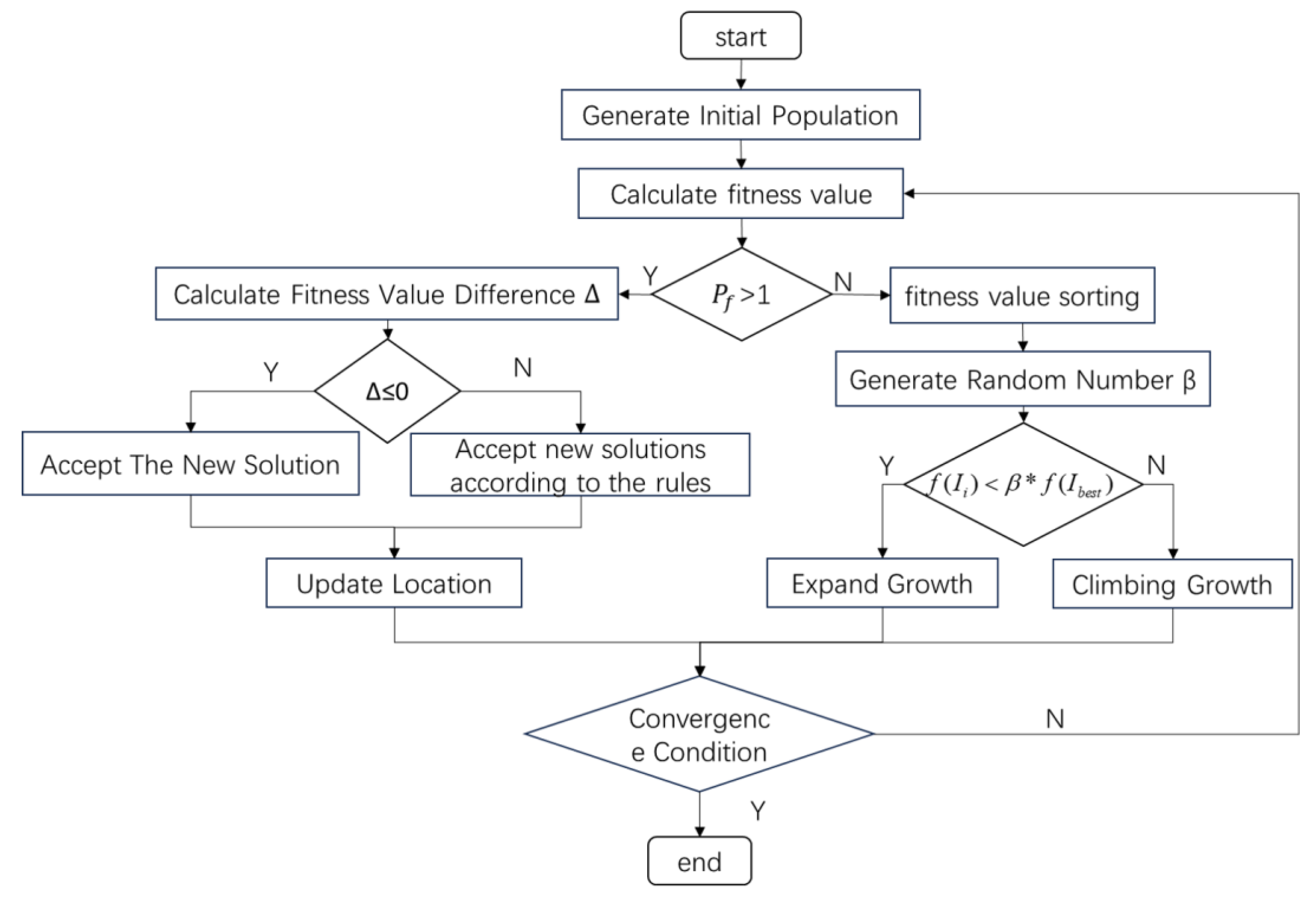
5.3. Ivy-SA Algorithm

The IVYA demonstrates strong convergence and wide applicability across various environments and input data. It features a flexible parameter adjustment mechanism that allows for the tuning of the optimization speed and accuracy according to specific problem requirements, making it suitable for tasks of varying scales and complexities. However, it is sensitive to the initial parameter values, and improper initialization can lead to slow convergence or result in suboptimal local solutions [38].

The SA algorithm is renowned for its powerful global search capability. By introducing randomness and accepting worse solutions with certain probabilities, it effectively escapes local optima and searches for the global optimum. The SA algorithm can be applied to a wide range of optimization problems, including both continuous and discrete problems, and is not sensitive to the initial solution, offering good robustness. However, its convergence speed is relatively slow, especially in high-dimensional spaces and near the optimal solution, where numerous iterations may be needed to obtain a stable solution [39].

The SA algorithm can effectively address the issue of the IVYA becoming stuck in local optima, whereas the IVYA can compensate for the slow convergence of the SA algorithm. This synergy between the two algorithms makes their combination highly beneficial. To harness the advantages of both methods, a balance factor $P_f$ is introduced. When $P_f>1$, the algorithm updates according to the SA algorithm, promoting global exploration. When $P_f\le 1$, the update follows the IVYA for faster convergence. The hybrid algorithm is named the Ivy-SA algorithm. A flowchart of the Ivy-SA algorithm is shown in Figure 5.

$$\left\{\begin{array}{c}{r}_1=B_f·(1-Iter/MaxIt)\\ r_2=rand\times 2\pi \\ P_f=|r_1\times sin(r_2\left)\right|\end{array}\right.$$

(49)

where $B_f$ is the balance constant, $Iter$ is the current iteration number, and $MaxIt$ is the maximum number of iterations.

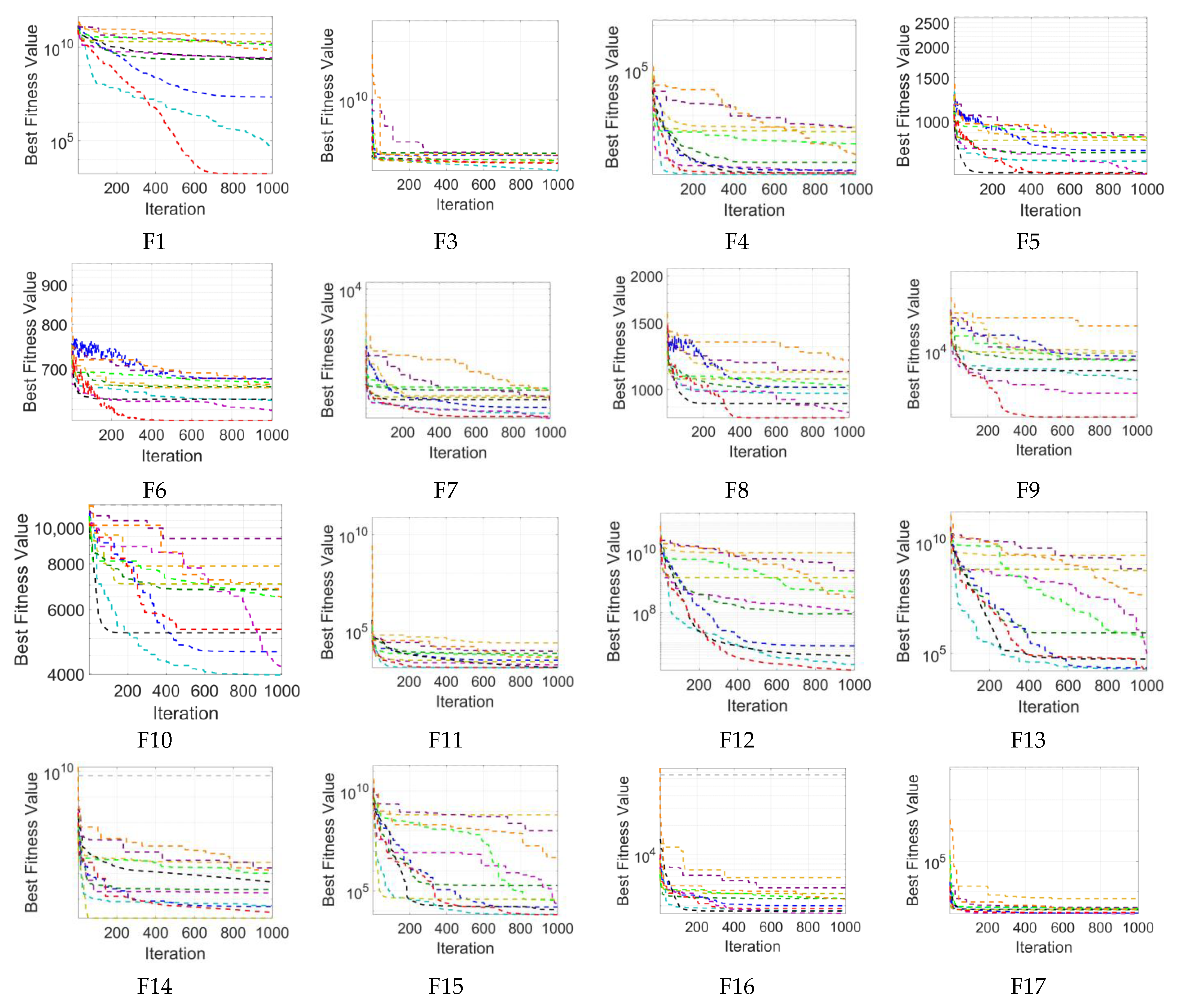
5.4. Ivy-SA Algorithm Testing

The CEC2017 function test suite, excluding F2, consists of 29 test functions that cover the following categories: Unimodal Functions (F1, F3), which assess the convergence performance of algorithms by evaluating their ability to find the globally unique optimal solution; Simple Multimodal Functions (F4–F10), which test the global exploration capability of algorithms by introducing multiple local extrema; Hybrid Functions (F11–F20), which combine multiple benchmark functions using rotation matrices and shifting operations, assigning different weights to sub-functions to create optimization surfaces with complex topologies; and Composition Functions (F21–F30), which further incorporate bias values and dynamic weights to integrate hybrid or benchmark functions into hierarchical problems, simulating the multi-scale challenges faced in practical engineering optimization. The CEC2017 benchmark function set increases the difficulty of finding suitable gradients and optimal solutions, making artificially designed problems closer to real-world scenarios and effectively avoiding unfairness caused by search biases.

To comprehensively evaluate the performance of the Ivy-SA algorithm, it is tested on the CEC2017 benchmark function set and compared with classical algorithms, including PSO (Particle Swarm Optimization), GA (Genetic Algorithm), GWO (Grey Wolf Optimizer), WOA (Whale Optimization Algorithm), CDO (Chernobyl Disaster Optimizer), SA (Simulated Annealing), as well as recently developed algorithms such as IVYA (Ivy Algorithm), CPO (Crested Porcupine Optimizer), HEOA (Human Evolutionary Optimization Algorithm), LEA (Love Evolution Algorithm), and NRBO (Newton-Raphson-Based Optimizer). To reduce the impact of randomness in the optimization process and improve the reliability of the test results, each algorithm is independently tested 30 times, and the mean and standard deviation (Std) of these 30 runs are calculated as comprehensive performance metrics. The mean reflects the solution accuracy of the algorithm and is used to assess its optimization capability; a lower mean indicates higher convergence precision and stronger optimization ability. The standard deviation represents the variability in the optimal values obtained by the algorithm, thereby evaluating its stability; a lower standard deviation indicates higher solution stability.

In the experiments, the population size was set to 30, the problem dimensionality to 30, and the number of iterations to 1000, with all algorithms configured consistently. The internal parameter settings for some of the algorithms are shown in

Table 3. Parameter settings.

Algorithm	Parameters
PSO	Learning factors c1 = 2, c2 = 2; the inertia factor wMax = 0.9; wMin = 0.6;
GA	Crossover probability pc = 0.8; mutation probability pm = 0.05;
WOA	Constant a = 2 − t × ((2)/Max_iter);
SA	Initial temperature T0 = 100; cooling coefficient alpha = 0.95;
CPO	Convergence rate alpha = 0.2; percentage of tradeoff Tf = 0.8;
HEOA	Warning value A = 0.6; leaders LN = 0.4; explorers EN = 0.4; followers FN = 0.1;
NRBO	Deciding factor DF = 0.6;
Ivy-SA	Balance factor Bf = 2

.

The results of various algorithms on the CEC2017 test suite are presented in

Table 4. Results of the different algorithms on the CEC2017 functions.

Function		PSO	GA	GWO	WOA	CDO	SA	IVY	CPO	HEOA	LEA	NRBO	Ivy-SA
F1	Mean	7.81 × 104	3.02 × 1010	2.69 × 109	1.73 × 109	5.24 × 1010	5.58 × 107	1.23 × 109	2.21 × 1010	1.23 × 1010	7.11 × 109	1.64 × 1010	* 1.79 × 104
	STD	1.14 × 105	1.45 × 1010	1.40 × 109	8.30 × 108	2.20 × 108	5.33 × 107	2.56 × 109	3.38 × 109	4.00 × 109	3.74 × 109	4.28 × 109	5.15 × 104
F3	Mean	1.63 × 104	2.90 × 105	4.66 × 104	2.52 × 105	8.69 × 104	1.55 × 105	5.86 × 104	1.48 × 105	6.54 × 104	2.22 × 105	4.88 × 104	3.92 × 104
	STD	6.46E+03	7.02 × 104	1.12 × 104	7.66 × 104	4.43 × 103	2.03 × 104	4.93 × 103	4.23 × 104	8.43 × 103	5.84 × 104	7.21 × 103	4.93 × 103
F4	Mean	4.79 × 102	5.76 × 103	5.99 × 102	8.42 × 102	5.43 × 103	5.86 × 102	6.47 × 102	4.31 × 103	1.59 × 103	1.05 × 103	1.95 × 103	5.03 × 102
	STD	1.64 × 101	3.38 × 103	7.18 × 101	1.42 × 102	1.09 × 102	2.98 × 101	5.20 × 102	1.30 × 103	6.86 × 102	2.90 × 102	9.14 × 102	1.67 × 101
F5	Mean	6.92 × 102	9.79 × 102	6.19 × 102	8.31 × 102	8.51 × 102	7.42 × 102	7.01 × 102	8.48 × 102	8.42 × 102	8.30 × 102	8.33 × 102	5.67 × 102
	STD	3.82 × 101	7.76 × 101	2.42 × 101	6.12 × 101	1.64 × 101	3.68 × 101	4.41 × 101	2.51 × 101	3.58 × 101	5.51 × 101	4.10 × 101	3.61 × 101
F6	Mean	6.47 × 102	7.17 × 102	6.11 × 102	6.77 × 102	6.70 × 102	6.80 × 102	6.21 × 102	6.67 × 102	6.75 × 102	6.79 × 102	6.71 × 102	6.00 × 102
	STD	7.45 × 100	1.50 × 101	4.43 × 100	1.18 × 101	4.89 × 100	5.75 × 100	1.90 × 101	8.41 × 100	6.85 × 100	1.34 × 101	8.62 × 100	1.49 × 10−
F7	Mean	9.27 × 102	1.84 × 103	8.97 × 102	1.30 × 103	1.31 × 103	1.08 × 103	1.15 × 103	1.25 × 103	1.34 × 103	1.41 × 103	1.22 × 103	8.05 × 102
	STD	6.21 × 101	2.20 × 102	5.41 × 101	7.81 × 101	2.16 × 101	4.76 × 101	1.12 × 102	5.51 × 101	6.96 × 101	1.51 × 102	7.79 × 101	4.68 × 101
F8	Mean	9.31 × 102	1.22 × 103	8.97 × 102	1.04 × 103	1.09 × 103	1.02 × 103	9.40 × 102	1.11 × 103	1.08 × 103	1.13 × 103	1.08 × 103	8.58 × 102
	STD	3.13 × 101	6.31 × 101	2.15 × 101	4.97 × 101	1.88 × 101	3.16 × 101	3.07 × 101	1.71 × 101	2.54 × 101	5.21 × 101	3.38 × 101	3.15 × 101
F9	Mean	4.90 × 103	8.57 × 103	2.30 × 103	1.17 × 104	9.56 × 103	7.75 × 103	5.10 × 103	1.00 × 104	8.00 × 103	1.80 × 104	6.82 × 103	9.85 × 102
	STD	1.14 × 103	1.83 × 103	9.14 × 102	4.47 × 103	1.07 × 103	1.68 × 103	4.52 × 102	1.91 × 103	9.51 × 102	4.59 × 103	1.32 × 103	1.03 × 102
F10	Mean	4.84 × 103	7.92 × 103	4.87 × 103	7.40 × 103	9.00 × 103	4.38 × 103	5.27 × 103	9.35 × 103	7.09 × 103	7.71 × 103	7.81 × 103	5.02 × 103
	STD	6.83 × 102	8.64 × 102	1.48 × 103	7.53 × 102	2.93 × 102	3.15 × 102	6.57 × 102	2.97 × 102	5.89 × 102	6.82 × 102	5.94 × 102	6.32 × 102
F11	Mean	1.22 × 103	1.99 × 104	2.89 × 103	6.31 × 103	2.04 × 104	3.13 × 103	1.28 × 103	7.92 × 103	4.04 × 103	7.85 × 103	2.53 × 103	1.20 × 103
	STD	3.82 × 101	1.16 × 104	1.34 × 103	2.90 × 103	6.92 × 103	7.46 × 102	1.93 × 102	2.11 × 103	1.55 × 103	2.52 × 103	6.75 × 102	4.44 × 101
F12	Mean	1.61 × 106	2.85 × 109	1.07 × 108	2.46 × 108	9.77 × 109	6.34 × 106	4.48 × 107	2.70 × 109	4.86 × 108	3.10 × 108	1.20 × 109	1.58 × 106
	STD	1.07 × 106	2.95 × 109	1.05 × 108	1.54 × 108	8.34 × 107	4.33 × 106	2.26 × 108	1.03 × 109	3.89 × 108	1.31 × 108	5.41 × 108	1.19 × 106
F13	Mean	1.53 × 104	1.98 × 109	1.46 × 107	1.92 × 106	2.40 × 109	2.65 × 104	4.23 × 104	7.92 × 108	2.19 × 106	5.15 × 107	2.41 × 108	4.28 × 104
	STD	1.33 × 104	2.39 × 109	3.64 × 107	1.72 × 106	1.20 × 108	9.43 × 103	1.86 × 104	3.83 × 108	2.27 × 106	4.03 × 107	1.71 × 108	2.21 × 104
F14	Mean	2.78 × 104	1.26 × 107	4.83 × 105	1.46 × 106	2.68 × 106	4.03 × 104	8.34 × 105	1.69 × 106	1.34 × 106	1.66 × 106	2.32 × 105	6.80 × 104
	STD	2.55 × 104	1.36 × 107	4.79 × 105	1.65 × 106	1.09 × 105	3.11 × 104	7.10 × 105	1.03 × 106	7.20 × 105	1.50 × 106	4.05 × 105	5.18 × 104
F15	Mean	5.02 × 103	7.26 × 107	1.32 × 106	1.20 × 106	6.52 × 108	1.54 × 104	2.00 × 106	7.24 × 107	1.11 × 106	6.33 × 106	2.39 × 106	1.18 × 104
	STD	3.36 × 103	1.63 × 108	3.15 × 106	2.07 × 106	2.02 × 105	5.95 × 103	1.05 × 107	4.24 × 107	1.28 × 106	9.28 × 106	5.77 × 106	6.22 × 103
F16	Mean	2.72 × 103	4.12 × 103	2.57 × 103	4.16 × 103	7.98 × 103	2.73 × 103	2.94 × 103	4.59 × 103	3.76 × 103	3.61 × 103	3.87 × 103	2.36 × 103
	STD	2.82 × 102	5.50 × 102	2.72 × 102	4.80 × 102	1.73 × 103	2.20 × 102	3.61 × 102	2.21 × 102	4.89 × 102	3.98 × 102	4.60 × 102	2.52 × 102
F17	Mean	2.40 × 103	3.04 × 103	2.10 × 103	2.75 × 103	1.59 × 104	2.09 × 103	2.57 × 103	3.01 × 103	2.55 × 103	2.77 × 103	2.61 × 103	1.92 × 103
	STD	3.23 × 102	3.09 × 102	2.05 × 102	3.17 × 102	1.40 × 104	9.51 × 101	3.19 × 102	1.61 × 102	2.40 × 102	2.86 × 102	2.23 × 102	1.78 × 102
F18	Mean	5.29 × 105	1.49 × 107	2.31 × 106	9.96 × 106	9.02 × 106	5.02 × 105	7.34 × 105	2.32 × 107	6.62 × 106	1.36 × 107	1.89 × 106	4.09 × 105
	STD	4.78 × 105	1.56 × 107	4.13 × 106	1.30 × 107	1.08 × 106	3.13 × 105	6.15 × 105	2.07 × 107	5.46 × 106	1.44 × 107	2.91 × 106	2.58 × 105
F19	Mean	9.47 × 103	3.31 × 107	8.34 × 105	1.11 × 107	1.37 × 108	4.49 × 105	1.35 × 106	9.98 × 107	5.83 × 106	2.55 × 107	1.82 × 107	1.55 × 104
	STD	9.79 × 103	4.97 × 107	8.99 × 105	9.23 × 106	5.45 × 106	6.05 × 105	5.12 × 106	7.66 × 107	3.43 × 106	1.97 × 107	1.77 × 107	1.43 × 104
F20	Mean	2.63 × 103	3.22 × 103	2.49 × 103	2.91 × 103	2.99 × 103	2.54 × 103	2.71 × 103	3.24 × 103	2.71 × 103	2.93 × 103	2.81 × 103	2.40 × 103
	STD	1.87 × 102	2.80 × 102	1.49 × 102	2.48 × 102	1.34 × 102	8.81 × 101	2.51 × 102	1.52 × 102	1.61 × 102	2.38 × 102	1.66 × 102	1.46 × 102
F21	Mean	2.48 × 103	2.84 × 103	2.41 × 103	2.60 × 103	2.63 × 103	2.52 × 103	2.40 × 103	2.63 × 103	2.60 × 103	2.60 × 103	2.59 × 103	2.36 × 103
	STD	2.74 × 101	6.79 × 101	3.48 × 101	4.46 × 101	1.71 × 101	4.10 × 101	3.92 × 101	2.58 × 101	4.70 × 101	3.90 × 101	5.11 × 101	2.83 × 101
F22	Mean	5.15 × 103	9.90 × 103	5.61 × 103	7.74 × 103	1.00 × 104	3.67 × 103	4.29 × 103	6.41 × 103	6.65 × 103	6.21 × 103	6.07 × 103	2.68 × 103
	STD	2.30 × 103	9.88 × 102	1.68 × 103	1.74 × 103	9.78 × 102	1.62 × 103	2.39 × 103	1.75 × 103	1.81 × 103	2.71 × 103	2.25 × 103	1.17 × 103
F23	Mean	3.24 × 103	3.49 × 103	2.76 × 103	3.09 × 103	3.69 × 103	2.94 × 103	2.80 × 103	3.19 × 103	3.12 × 103	2.97 × 103	3.07 × 103	2.70 × 103
	STD	1.33 × 102	1.76 × 102	3.17 × 101	9.63 × 101	7.10 × 101	5.94 × 101	5.53 × 101	6.20 × 101	1.23 × 102	5.45 × 101	5.71 × 101	2.72 × 101
F24	Mean	3.23 × 103	3.74 × 103	2.96 × 103	3.23 × 103	3.82 × 103	3.04 × 103	2.96 × 103	3.37 × 103	3.18 × 103	3.11 × 103	3.19 × 103	2.90 × 103
	STD	9.49 × 101	1.70 × 102	6.18 × 101	1.09 × 102	5.54 × 101	1.16 × 102	6.36 × 101	7.46 × 101	9.84 × 101	6.24 × 101	6.18 × 101	2.38 × 101
F25	Mean	2.88 × 103	5.32 × 103	3.01 × 103	3.11 × 103	3.58 × 103	3.03 × 103	2.93 × 103	3.81 × 103	3.20 × 103	3.54 × 103	3.41 × 103	2.90 × 103
	STD	9.86 × 100	9.69 × 102	4.13 × 101	5.07 × 101	2.38 × 101	2.70 × 101	3.74 × 101	2.02 × 102	1.17 × 102	2.21 × 102	2.62 × 102	1.44 × 101
F26	Mean	6.40 × 103	9.50 × 103	4.68 × 103	8.16 × 103	8.64 × 103	3.86 × 103	7.08 × 103	8.35 × 103	8.26 × 103	7.28 × 103	7.55 × 103	3.46 × 103
	STD	2.05 × 103	9.64 × 102	4.92 × 102	1.22 × 103	2.28 × 102	3.59 × 102	1.22 × 103	7.36 × 102	1.45 × 103	5.28 × 102	1.11 × 103	7.31 × 102
F27	Mean	3.49 × 103	4.23 × 103	3.26 × 103	3.45 × 103	3.63 × 103	3.34 × 103	3.32 × 103	3.85 × 103	3.41 × 103	3.36 × 103	3.42 × 103	3.22 × 103
	STD	2.90 × 102	2.81 × 102	2.95 × 101	1.27 × 102	3.73 × 101	2.37 × 101	9.79 × 101	1.09 × 102	1.10 × 102	6.83 × 101	7.04 × 101	1.01 × 101
F28	Mean	3.23 × 103	6.61 × 103	3.52 × 103	3.57 × 103	5.01 × 103	3.39 × 103	3.27 × 103	5.04 × 103	4.10 × 103	3.95 × 103	4.11 × 103	3.21 × 103
	STD	2.21 × 101	1.46 × 103	1.67 × 102	1.08 × 102	2.15 × 101	4.06 × 101	3.39 × 101	3.64 × 102	3.22 × 102	3.26 × 102	5.43 × 102	1.57 × 101
F29	Mean	4.17 × 103	5.89 × 103	3.88 × 103	5.24 × 103	6.21 × 103	4.22 × 103	4.25 × 103	5.52 × 103	5.33 × 103	5.09 × 103	4.97 × 103	3.67 × 103
	STD	3.02 × 102	9.15 × 102	1.92 × 102	4.24 × 102	3.09 × 102	1.72 × 102	3.06 × 102	2.82 × 102	4.76 × 102	4.86 × 102	4.41 × 102	1.78 × 102
F30	Mean	2.94 × 104	3.82 × 107	1.48 × 107	5.15 × 107	2.86 × 109	2.06 × 106	1.55 × 105	1.30 × 108	5.68 × 107	4.12 × 107	6.51 × 107	1.19 × 105
	STD	1.15 × 104	4.20 × 107	1.40 × 107	2.77 × 107	8.15 × 108	1.67 × 106	1.53 × 105	6.33 × 107	3.75 × 107	3.04 × 107	4.80 × 107	9.17 × 104

* Bold data indicates the best performance among all algorithms.

, with boldface data indicating the best performance among all algorithms. It can be observed from the data that, in unimodal functions, the Ivy-SA algorithm exhibits excellent performance in both mean and standard deviation for F1, with only the mean value for F3 being slightly lower than that of the PSO algorithm. This indicates good convergence and stability in unimodal functions. In simple multimodal functions, the mean and standard deviation of the Ivy-SA algorithm are generally lower than those of the other algorithms. For example, in F6 the mean is 6.00 × 10² and the standard deviation is 1.49 × 10⁻², demonstrating its ability to effectively balance global and local searches and avoid local optima. In hybrid functions, Ivy-SA continues to perform well; for instance, in F11, the mean is 1.2 × 10³ and the standard deviation is 44.4, showing a clear advantage over the other algorithms, which suggests that it can adeptly handle the challenges presented by complex hybrid functions. Finally, in composition functions, the Ivy-SA algorithm still performs outstandingly. For example, in F21, the mean is 2.36 × 10³ and the standard deviation is 28.3, indicating that when dealing with complex problems composed of multiple different functions, it can effectively coordinate and optimize all components to achieve the overall optimal solution.

Through the Friedman test, the performance of each algorithm is ranked, with the results shown in

Table 5. Results of the Friedman test.

Function	PSO	GA	GWO	WOA	CDO	SA	IVY	CPO	HEOA	LEA	NRBO	Ivy-SA
F1	3	12	2	8	9	4	5	7	10	11	6	1
F3	3	12	2	6	9	5	4	10	7	11	8	1
F4	3	8	2	9	10	6	4	11	7	12	5	1
F5	3	10	2	7	11	1	5	12	6	8	9	4
F6	2	11	5	8	12	6	3	9	7	10	4	1
F7	2	10	5	6	12	4	3	11	8	7	9	1
F8	1	11	5	6	12	2	3	10	7	8	9	4
F9	1	12	5	7	11	2	6	10	8	9	4	3
F10	1	10	5	7	12	3	4	11	8	9	6	2
F11	3	9	2	10	12	4	5	11	7	6	8	1
F12	4	10	3	8	12	2	6	11	5	9	7	1
F13	3	10	6	7	11	2	4	12	8	9	5	1
F14	1	10	5	7	12	4	3	11	6	9	8	2
F15	4	11	2	8	10	3	5	12	6	9	7	1
F16	4	12	3	8	11	5	2	10	7	9	6	1
F17	4	11	5	10	12	2	3	8	9	6	7	1
F18	10	11	2	8	12	4	3	9	7	5	6	1
F19	9	11	2	8	12	4	3	10	6	5	7	1
F20	1	12	4	6	10	5	3	11	7	9	8	2
F21	4	12	3	8	11	2	6	10	9	5	7	1
F22	6	12	2	9	10	4	3	11	7	5	8	1
F23	2	12	5	6	10	4	3	11	9	7	8	1
F24	3	11	2	8	12	4	5	10	9	7	6	1
F25	1	6	5	8	12	4	3	11	9	7	10	2
F26	3	12	2	8	9	4	5	7	10	11	6	1
F27	3	12	2	6	9	5	4	10	7	11	8	1
F28	3	8	2	9	10	6	4	11	7	12	5	1
F29	3	10	2	7	11	1	5	12	6	8	9	4
F30	2	11	5	8	12	6	3	9	7	10	4	1
MFr	3.07	10.83	3.52	7.59	10.86	4.03	3.90	10.10	7.52	8.03	7.07	1.48
Final rank	2	11	3	8	12	5	4	10	7	9	6	1

. Among the 29 test functions, the Ivy-SA algorithm demonstrates superior performance, outperforming all other algorithms on 20 functions and ranking first with an average score of 1.48. For functions F3, F4, F15, F19, F25, and F30, the performance of Ivy-SA is only surpassed by the PSO algorithm. In function F13, Ivy-SA ranks behind the PSO, SA, and IVY algorithms, and in function F14, its performance ranks after that of the PSO and SA algorithms. Overall, Ivy-SA exhibits strong optimization capabilities, performing well on the majority of test functions; even on some test functions where Ivy-SA does not rank first, it still outperforms most of the compared algorithms.

To provide a clearer visualization of the convergence behavior of the algorithms, Figure 6 presents the convergence curves of 12 algorithms on the CEC2017 benchmark test suite. From the convergence curves of functions F5, F8, F10, F15, F16, and F21, it is evident that the IVYA algorithm exhibits the highest rate of change in certain regions, indicating its capability for rapid convergence within those areas. The convergence curves for functions F5, F6, F8, F21, and F23 reveal that the SA algorithm initially undergoes oscillations, suggesting its propensity to accept inferior solutions with a certain probability during the global search phase before gradually converging. The development of optimization algorithms aims to balance early global exploration with later rapid convergence. Guided by this principle, the proposed Ivy-SA algorithm introduces a balance factor, inheriting the global search ability of the SA algorithm during the initial iterations and the swift convergence characteristic of the IVYA algorithm in the later stages, as demonstrated by the convergence curves of functions F5, F6, F7, F8, F10, F16, F21, F23, F24, and F26. Furthermore, the convergence curves for functions F8, F9, F13, F15, F18, F23, and F26 show that the IVYA algorithm experiences abrupt curvature changes during convergence and ultimately converges to the optimal solution, indicating its ability to escape local optima. Overall, the Ivy-SA algorithm effectively combines the SA algorithm’s capability to avoid local optima with the IVYA algorithm’s rapid convergence, leading to a significant enhancement in optimization performance.

5.5. Co-Optimization of Hybrid Power Systems

Ship diesel–electric hybrid power systems have attracted considerable attention in recent years. By integrating energy flows from fossil fuels and battery storage, these systems introduce renewed vitality into marine propulsion. This technology effectively reduces fuel consumption and plays a positive role in environmental protection. However, achieving optimal operational states for hybrid power systems remains a persistent challenge. Typically, hardware configuration and energy management parameters are optimized separately. This study attempts to co-optimize them to achieve an overall optimal system state.

The Ivy-SA algorithm is employed to optimize the hybrid power system. To further validate the effectiveness of the Ivy-SA algorithm in addressing hybrid power system optimization problems, comparative analyses are conducted with PSO, GWO, IVYA, and SA algorithms, which ranked 2nd, 3rd, 4th, and 5th, respectively, in the Friedman test.

Under the ECMS, the hardware configuration and energy management parameters were optimized simultaneously under real-world operating conditions. The key parameters, including the exhaust manifold diameter, exhaust pipe diameter, intake/exhaust valve lift ratio, turbocharger compression ratio, mass flow rate, motor power, battery parallel quantity, DOD, and charge/discharge factor, were selected in the optimization process. The optimization process was implemented using the SA algorithm, IVYA, and Ivy-SA algorithm, with a population size of 30 and 500 iterations. Under the ECMS-based control strategy and considering real-world operating conditions, parameters such as exhaust manifold diameter, exhaust pipe diameter, intake and exhaust valve lift ratio, turbocharger compression ratio and mass flow rate, motor power, number of battery parallel connections, depth of discharge, and charge/discharge factors are selected for optimization. The population size is set to 30 with 500 iterations.

Based on the life cycle cost, five algorithms have optimized the system to varying degrees, demonstrating different choices in parameter configuration. The results, as shown in

Table 6. Co-optimization results.

Parameter	Initial Value	PSO	GWO	IVYA	SA	Ivy-SA
Exhaust Manifold	200	180	180	180	180	180
Exhaust Pipe	160	162	168	158	155	165
Intake Valve Lift Ratio	3.055	3.345	3.345	3.345	3.345	3.345
Exhaust Valve Lift Ratio	3.055	3.194	3.194	3.194	3.194	3.194
Compressor Pressure Ratio	6.3	6.1	9.1	5.98	7.4	6.3
Compressor Mass Flow Rate	14.2	11.8	15.2	14.5	13.3	14.2
Bore	460	442	448	448	467	455
Stroke	580	603	595	595	571	586
Motor Rated Power	2550	2983	1925	2078	2031	2813
Number of Parallel Batteries	88	121	62	78	72	113
Depth of Discharge	80	88	74	84	78	84
Charge Efficiency Factor	1.7	1.63	1.78	1.62	1.82	1.66
Discharge Efficiency Factor	2.3	1.95	2.06	1.93	2.18	1.97
CO₂ Emissions (ton)	41.86	35.80	40.53	37.52	40.53	34.50
Battery Energy Consumption (kWh)	2875.46	2983.34	1268.08	1682.45	2134.92	2402.33
Fuel Consumption (ton)	12.85	10.98	12.44	11.51	12.44	11.03
LCC ($)	1.28 × 108	1.11 × 108	1.21 × 108	1.13 × 108	1.22 × 108	1.09 × 108
Cost Savings	-	13.19%	5.30%	11.43%	4.13%	14.49%

, reveal the complexity of the system and the correlations among parameters.

In terms of hardware configuration, due to the approximately linear relationship between the exhaust manifold and BSFC, all five algorithms selected the same value. The impact of exhaust pipe diameter on BSFC varies under different conditions; influenced by comprehensive factors in actual operating conditions, the system exhibits multiple local optimal solutions. The PSO, GWO, and Ivy-SA algorithms increased the diameter to varying degrees, while the IVYA and SA algorithms decreased it to different extents. A higher intake and exhaust valve lift ratio results in a lower BSFC; therefore, all five algorithms chose the same value. Regarding turbocharger configuration, the PSO and IVYA algorithms reduced the compression ratio, whereas the GWO, SA, and Ivy-SA algorithms increased it, with all adjusting the mass flow rate. Although bore and stroke individually have clear patterns of influence on BSFC, when the engine displacement is constant, they exhibit strong coupling. The five algorithms selected different values but all opted to decrease the bore while increasing the stroke. In terms of battery and motor selection, the PSO and IVYA algorithms increased battery capacity and motor rated power, while the GWO, SA, and Ivy-SA algorithms reduced them.

Regarding energy management parameters, the depth of discharge significantly affects battery health. It can be observed that the larger the battery capacity chosen by different algorithms, the more stable the instantaneous discharge current of individual cells when delivering the same power, allowing for a greater depth of discharge. The charge-discharge equivalence factor determines the cost of electrical energy in the energy management strategy; a larger value indicates a higher electricity cost. The GWO and SA algorithms selected a larger charge/discharge factor due to their choice of lower battery capacity, making the entire journey more dependent on the engine. Although this reduces battery procurement costs, it increases fuel consumption, resulting in less optimized total costs. The IVYA algorithm, despite choosing a lower charge/discharge factor, increased battery cycle times due to its lower battery capacity configuration, also increasing diesel generator operation during cycles. The PSO and Ivy-SA algorithms selected larger battery capacities and lower charge-discharge factors, achieving better optimization results. However, from a comprehensive perspective, the Ivy-SA algorithm attains the optimal outcome.

Overall, due to the system’s complexity and the coupling relationships among parameters, the PSO, GWO, IVYA, SA, and Ivy-SA algorithms achieved varying degrees of system optimization, reducing total costs by 13.19%, 5.30%, 11.43%, 4.13%, and 14.49%, respectively, further demonstrating the effectiveness of the Ivy-SA algorithm.

6. Conclusions

On the basis of the complex energy flow relationships within series—parallel hybrid power systems, detailed main engine and hybrid ship models were established, and their accuracy was validated. To ensure instantaneous energy allocation at various levels of the ship, an ECMS-based energy management strategy was formulated, which enables efficient energy management.

The performance of a ship’s hybrid power system depends on multiple factors. It is essential to consider the hardware configuration for optimal compatibility, such as engine performance and battery capacity, as well as the appropriate energy control strategy and corresponding parameters. To address the complex issue of co-optimizing the system hardware configuration and energy management parameters, a hybrid Ivy-SA algorithm was developed. The algorithm was tested with the CEC2017 benchmark suite, and the results demonstrate that the optimal solution of the Ivy-SA algorithm is better than those of the other 11 algorithms. The Ivy-SA algorithm has both the fast convergence speed of the IVYA and the ability of the SA algorithm to escape local optima.

On the basis of the system’s lifecycle cost, the hardware configuration, and the energy management parameters of the hybrid power system were co-optimized with the PSO, GWO, IVYA, SA, and Ivy-SA algorithms. The results indicate that the Ivy-SA algorithm achieves the most economic performance among the four algorithms, effectively reducing the total lifecycle expenditure of the ship.

In this paper, the hardware parameters and control parameters of the hybrid power system were co-optimized through simulation calculations. In the future, the effectiveness of the Ivy-SA algorithm’s optimization results can be further validated through hardware-in-the-loop experiments and experiments involving real ships. Additionally, the applicability of the Ivy-SA algorithm for other problems in the field of ship and marine engineering could be explored.

References

1. Inal, O.B.; Charpentier, J.-F.; Deniz, C. Hybrid power and propulsion systems for ships: Current status and future challenges. Renew. Sustain. Energy Rev. 2022, 156, 111965. [Google Scholar]
2. Wu, P.; Bucknall, R. Hybrid fuel cell and battery propulsion system modelling and multi-objective optimisation for a coastal ferry. Int. J. Hydrog. Energy 2020, 45, 3193–3208. [Google Scholar]
3. Wang, Y.; Iris, Ç. Transition to near-zero emission shipping fleet powered by alternative fuels under uncertainty. Transp. Res. Part D Transp. Environ. 2025, 142, 104689. [Google Scholar]
4. Zhang, C. The research of power allocation in diesel-electric hybrid propulsion system. In Proceedings of the 2019 Chinese Automation Congress (CAC), Hangzhou, China, 22–24 November 2019; pp. 3664–3668. [Google Scholar]
5. Zaccone, R.; Campora, U.; Martelli, M. Optimisation of a diesel-electric ship propulsion and power generation system using a genetic algorithm. J. Mar. Sci. Eng. 2021, 9, 587. [Google Scholar] [CrossRef]
6. Tadros, M.; Ventura, M.; Soares, C.G. Optimization procedure to minimize fuel consumption of a four-stroke marine turbocharged diesel engine. Energy 2019, 168, 897–908. [Google Scholar]
7. Liu, L.; Wang, X.; Liu, D.; Mao, W.; Xiong, F. Research on combustion process optimization of marine diesel engines based on dual-injector system. J. Phys. Conf. Ser. 2024, 2683, 012019. [Google Scholar]
8. Chen, X.; Liu, L.; Du, J.; Liu, D.; Huang, L.; Li, X. Intelligent optimization based on a virtual marine diesel engine using GA-ICSO hybrid algorithm. Machines 2022, 10, 227. [Google Scholar] [CrossRef]
9. Li, X.; Pan, L.; Zhang, J.; Jin, Z.; Jiang, W.; Wang, Y.; Liu, L.; Tang, R.; Lai, J.; Yang, X. A novel capacity allocation method for hybrid energy storage system for electric ship considering life cycle cost. J. Energy Storage 2025, 116, 116070. [Google Scholar]
10. Barrera-Cardenas, R.; Mo, O.; Guidi, G. Optimal sizing of battery energy storage systems for hybrid marine power systems. In Proceedings of the 2019 IEEE Electric Ship Technologies Symposium (ESTS), Washington, DC, USA, 14–16 August 2019; pp. 293–302. [Google Scholar]
11. Balci, G.; Phan, T.T.N.; Surucu-Balci, E.; Iris, Ç. A roadmap to alternative fuels for decarbonising shipping: The case of green ammonia. Res. Transp. Bus. Manag. 2024, 53, 101100. [Google Scholar]
12. Antonopoulos, S.; Visser, K.; Kalikatzarakis, M.; Reppa, V. MPC framework for the energy management of hybrid ships with an energy storage system. J. Mar. Sci. Eng. 2021, 9, 993. [Google Scholar] [CrossRef]
13. Liu, B.; Gao, D.; Yang, P.; Hu, Y. An energy efficiency optimization strategy of hybrid electric ship based on working condition prediction. J. Mar. Sci. Eng. 2022, 10, 1746. [Google Scholar] [CrossRef]
14. Wang, X.; Yuan, Y.; Tong, L.; Yuan, C.; Shen, B.; Long, T. Energy Management Strategy for Diesel–Electric Hybrid Ship Considering Sailing Route Division Based on DDPG. IEEE Trans. Transp. Electrif. 2023, 10, 187–202. [Google Scholar] [CrossRef]
15. Gao, D.; Wang, X.; Wang, T.; Wang, Y.; Xu, X. An energy optimization strategy for hybrid power ships under load uncertainty based on load power prediction and improved NSGA-II algorithm. Energies 2018, 11, 1699. [Google Scholar] [CrossRef]
16. Tjandra, R.; Wen, S.; Zhou, D.; Tang, Y. Optimal sizing of BESS for hybrid electric ship using multi-objective particle swarm optimization. In Proceedings of the 2019 10th International Conference on Power Electronics and ECCE Asia (ICPE 2019-ECCE Asia), Busan, Republic of Korea, 27–30 May 2019; pp. 1460–1466. [Google Scholar]
17. Xiang, Y.; Yang, X. An ECMS for multi-objective energy management strategy of parallel diesel electric hybrid ship based on ant colony optimization algorithm. Energies 2021, 14, 810. [Google Scholar] [CrossRef]
18. Chen, L.; Gao, D.; Xue, Q. Energy Management Strategy of Hybrid Ships Using Nonlinear Model Predictive Control via a Chaotic Grey Wolf Optimization Algorithm. J. Mar. Sci. Eng. 2023, 11, 1834. [Google Scholar] [CrossRef]
19. Shang, Q.; Sun, Y.; Zhou, Y.; Yan, L.; Wei, C.; Hu, W. Exploring the optimization of energy management strategy for hybrid ships based on the Grey Wolf optimization algorithm. In Proceedings of the 2023 7th International Conference on Transportation Information and Safety (ICTIS), Xi’an, China, 4–6 August 2023; pp. 298–305. [Google Scholar]
20. Liu, Z.; Munnannur, A. Design and development of heavy duty diesel engines. In Future Diesel Engines; Springer: Singapore, 2019; pp. 887–914. [Google Scholar]
21. Reitz, R.; Rutland, C. Development and testing of diesel engine CFD models. Prog. Energy Combust. Sci. 1995, 21, 173–196. [Google Scholar] [CrossRef]
22. Kim, K.-H.; Kong, K.-J. One-dimensional gas flow analysis of the intake and exhaust system of a single cylinder diesel engine. J. Mar. Sci. Eng. 2020, 8, 1036. [Google Scholar] [CrossRef]
23. Molland, A.F.; Turnock, S.R.; Hudson, D.A. Ship Resistance and Propulsion; Cambridge University Press: Cambridge, UK, 2017. [Google Scholar]
24. Zahedi, B.; Norum, L.E. Modeling and simulation of all-electric ships with low-voltage DC hybrid power systems. IEEE Trans. Power Electron. 2012, 28, 4525–4537. [Google Scholar] [CrossRef]
25. Paganelli, G.; Delprat, S.; Guerra, T.-M.; Rimaux, J.; Santin, J.-J. Equivalent consumption minimization strategy for parallel hybrid powertrains. In Proceedings of the Vehicular Technology Conference, IEEE 55th Vehicular Technology Conference, VTC Spring 2002 (Cat. No. 02CH37367), Birmingham, AL, USA, 6–9 May 2002; pp. 2076–2081. [Google Scholar]
26. Onori, S.; Serrao, L.; Rizzoni, G.; Onori, S.; Serrao, L.; Rizzoni, G. Pontryagin’s minimum principle. In Hybrid Electric Vehicles: Energy Management Strategies; Springer: London, UK, 2016; pp. 51–63. [Google Scholar]
27. Musardo, C.; Rizzoni, G.; Guezennec, Y.; Staccia, B. A-ECMS: An adaptive algorithm for hybrid electric vehicle energy management. Eur. J. Control 2005, 11, 509–524. [Google Scholar] [CrossRef]
28. Serrao, L.; Onori, S.; Rizzoni, G. ECMS as a realization of Pontryagin’s minimum principle for HEV control. In Proceedings of the 2009 American Control Conference, St. Louis, MO, USA, 10–12 June 2009; pp. 3964–3969. [Google Scholar]
29. Nejatzadegan, F.; Sobhani, V.; Pahlavan, M.; Dehghan, A. Effect of exhaust manifold geometry design on the performance of an internal combustion engine. Int. Commun. Heat Mass Transf. 2025, 162, 108593. [Google Scholar]
30. Sawant, P.; Warstler, M.; Bari, S. Exhaust tuning of an internal combustion engine by the combined effects of variable exhaust pipe diameter and an exhaust valve timing system. Energies 2018, 11, 1545. [Google Scholar] [CrossRef]
31. Balmelli, M.; Zsiga, N.; Merotto, L.; Soltic, P. Effect of the intake valve lift and closing angle on part load efficiency of a spark ignition engine. Energies 2020, 13, 1682. [Google Scholar] [CrossRef]
32. Kim, J.; Kim, H.; Yoon, S.; Sa, S.; Kim, W. Effect of valve timing and lift on flow and mixing characteristics of a CAI engine. Int. J. Automot. Technol. 2007, 8, 687–696. [Google Scholar]
33. Alrwashdeh, S.S.; Almajali, M.R.; Alsaraireh, F.M.; Ala’M, A.-F. Green performance enhancement of marine engines via turbocharger compression ratio optimization. Results Eng. 2024, 24, 102989. [Google Scholar] [CrossRef]
34. Xin, R.; Zhai, J.; Liao, C.; Wang, Z.; Zhang, J.; Bazari, Z.; Ji, Y. Simulation Study on the Performance and Emission Parameters of a Marine Diesel Engine. J. Mar. Sci. Eng. 2022, 10, 985. [Google Scholar] [CrossRef]
35. Zhang, Z.; Feng, H.; Jia, B.; Zuo, Z.; Smallbone, A.; Roskilly, A.P. Effect of the stroke-to-bore ratio on the performance of a dual-piston free piston engine generator. Appl. Therm. Eng. 2021, 185, 116456. [Google Scholar] [CrossRef]
36. Li, Y.; Liu, X.; Zhao, Y.; He, T.; Zeng, H. Optimization design of hybrid energy storage capacity configuration for electric ship. Energy Rep. 2024, 11, 887–894. [Google Scholar] [CrossRef]
37. Schmalstieg, J.; Käbitz, S.; Ecker, M.; Sauer, D.U. A holistic aging model for Li (NiMnCo) O2 based 18650 lithium-ion batteries. J. Power Sources 2014, 257, 325–334. [Google Scholar] [CrossRef]
38. Ghasemi, M.; Zare, M.; Trojovský, P.; Rao, R.V.; Trojovská, E.; Kandasamy, V. Optimization based on the smart behavior of plants with its engineering applications: Ivy algorithm. Knowl.-Based Syst. 2024, 295, 111850. [Google Scholar] [CrossRef]
39. Metropolis, N.; Rosenbluth, A.W.; Rosenbluth, M.N.; Teller, A.H.; Teller, E. Equation of state calculations by fast computing machines. J. Chem. Phys. 1953, 21, 1087–1092. [Google Scholar]
40. Kirkpatrick, S.; Gelatt, C.D., Jr.; Vecchi, M.P. Optimization by simulated annealing. Science 1983, 220, 671–680. [Google Scholar] [PubMed]
Figure 1. Simulation modeling.
Jmse 13 00731 g001
Figure 2. Model validation.
Jmse 13 00731 g002
Figure 3. Power allocation.
Jmse 13 00731 g003
Figure 4. Parameter sensitivity analysis.
Jmse 13 00731 g004
Figure 5. Flowchart of the Ivy-SA algorithm.
Jmse 13 00731 g005
Figure 6. Convergence curves of the three algorithms.
Jmse 13 00731 g006aJmse 13 00731 g006b