1. Introduction
Catch per unit effort (CPUE) is a crucial index for assessing the relative abundance of fishery resources, playing an essential role in monitoring stock fluctuations and informing fisheries management strategies [
1,
2]. CPUE data are collected from both survey-based research and commercial fisheries, with the former generally offering greater reliability. However, due to the challenges of obtaining extensive and continuous survey data, CPUE standardization often relies on commercial catch data, which are influenced by various environmental and anthropogenic factors such as spatiotemporal variability, gear type, fishing efficiency, and behavioral patterns.
Among the various explanatory variables used in CPUE standardization, the year effect plays a central role. It is generally assumed that once other sources of variation—such as spatial distribution, vessel characteristics, and socioeconomic or environmental factors—are accounted for, the estimated year effect serves as a proxy for interannual changes in stock abundance [
1]. This assumption underpins the value of CPUE standardization in monitoring population dynamics, especially in data-limited fisheries where independent biomass estimates are unavailable. Therefore, it is essential to identify and account for confounding influences to reduce uncertainty in CPUE-based indices [
3,
4,
5]. CPUE standardization has been conducted using various statistical approaches, including generalized linear models (GLM), generalized additive models (GAM), and generalized linear mixed models (GLMM) [
4,
6].
Global fishery resources are affected by various factors, including overfishing, climate change, marine pollution, global pandemics (COVID-19), and market fluctuations, which contribute to ongoing changes in fishery production and the broader fisheries economy [
7]. The COVID-19 pandemic has heightened economic uncertainty in the fisheries sector by disrupting global fisheries supply chains, reducing demand, causing logistical disruptions, and leading to a diminished workforce [
8,
9,
10]. These socioeconomic shifts, including the impact of COVID-19, have affected not only the production of specific fisheries and species but also the structure of supply chains and market stability. Furthermore, these disruptions pose a significant risk to food security and livelihoods, potentially triggering a cascading chain of disorder [
11,
12]. Therefore, conventional fisheries assessment and management approaches may be insufficient to effectively respond to the changing environmental and socioeconomic conditions, necessitating more sophisticated analytical frameworks and adaptive strategies [
13,
14].
The red snow crab (
Chionoecetes japonicus) is a crustacean belonging to the genus
Chionoecetes in the family Oregoniidae [
15]. It is mainly distributed in the deep waters of the coastal waters of South Korea and Japan [
16,
17]. In South Korea, red snow crab is a commercially valuable species, particularly in offshore fisheries, where recent socioeconomic changes have led to significant fluctuations in catch volumes and distribution patterns [
18].
The total red snow crab catch in South Korea increased from approximately 30,000 tons in 2010 to 41,000 tons in 2015 but subsequently declined to 15,000 tons by 2020. However, in 2023, it showed signs of recovery, reaching 31,500 tons [
19]. The species is primarily harvested in the Gangwon (GW) and Gyeongbuk (GB) regions, with around 80% processed as fresh seafood for both domestic consumption and export, mainly to Japan, the United States, and Europe. However, the COVID-19 pandemic severely disrupted the export of processed crab products, leading to a decline in factory operations and a sharp drop in fresh crab prices [
19]. These disruptions in the market and distribution networks, along with other external factors, resulted in increased economic losses in the fishery sector and contributed to a decline in catch volume.
South Korea’s red snow crab fishery is predominantly dependent on offshore trap fisheries, which accounted for an average of 80.7% of the total catch over the past five years (2019–2023), followed by coastal gillnet fisheries (9.7%) and coastal trap fisheries (9.1%) [
19]. This structural reliance suggests that socioeconomic changes could significantly influence production and distribution. The restructuring of distribution channels following the COVID-19 pandemic has also led to notable shifts in the market share of live versus fresh crab sales. The proportion of live crabs steadily increased from 2.8% in 2010 to 31.9% in 2019 and remained at 22.2% in 2023. Conversely, the share of fresh crabs declined from 97.2% in 2010 to 68.1% in 2019 but rebounded to 77.8% in 2023 [
19]. These shifts suggest that fluctuations in the red snow crab market are driven not only by variations in catch volume but also by broader socioeconomic dynamics.
Research on red snow crab in South Korea has primarily focused on biological and ecological aspects, such as maturation and spawning [
20], reproductive and distribution characteristics [
21], and variations in fishing grounds [
18]. In terms of resource assessment and fisheries management, previous studies have applied surplus production models for comparative analysis [
22] and bioeconomic models to evaluate the effectiveness of fisheries management strategies [
23]. However, most of these studies have overlooked the direct influence of socioeconomic factors on resource fluctuations. Even when economic indicators were considered, they often failed to capture the fundamental drivers of these changes. While CPUE standardization studies have incorporated environmental factors such as sea temperature, chlorophyll-a concentration, and lunar illumination, as well as regulatory measures like fishing closures and catch composition [
6,
24,
25,
26], there has been a lack of research integrating socioeconomic factors such as export volume fluctuations and the impact of COVID-19.
This study aims to improve the accuracy of CPUE estimation for red snow crab by incorporating socioeconomic factors, which have often been overlooked in previous studies. Using data from 2009 to 2023, this study focuses on the primary offshore trap fishing grounds of Gangwon (GW) and Gyeongbuk (GB). In addition to spatiotemporal factors, key socioeconomic variables—including the proportion of live catch, oil prices, global export prices, and the impact of the COVID-19 pandemic—were included as key explanatory variables. CPUE was standardized using a generalized additive model (GAM), and six different models were developed to determine the optimal predictor variables. Furthermore, through a stepwise approach, this study evaluates the impact of socioeconomic variables on CPUE variability. The findings emphasize the need to integrate socioeconomic considerations into resource assessments and provide valuable insights for sustainable fisheries management and policymaking.
2. Materials and Methods
2.1. Study Area
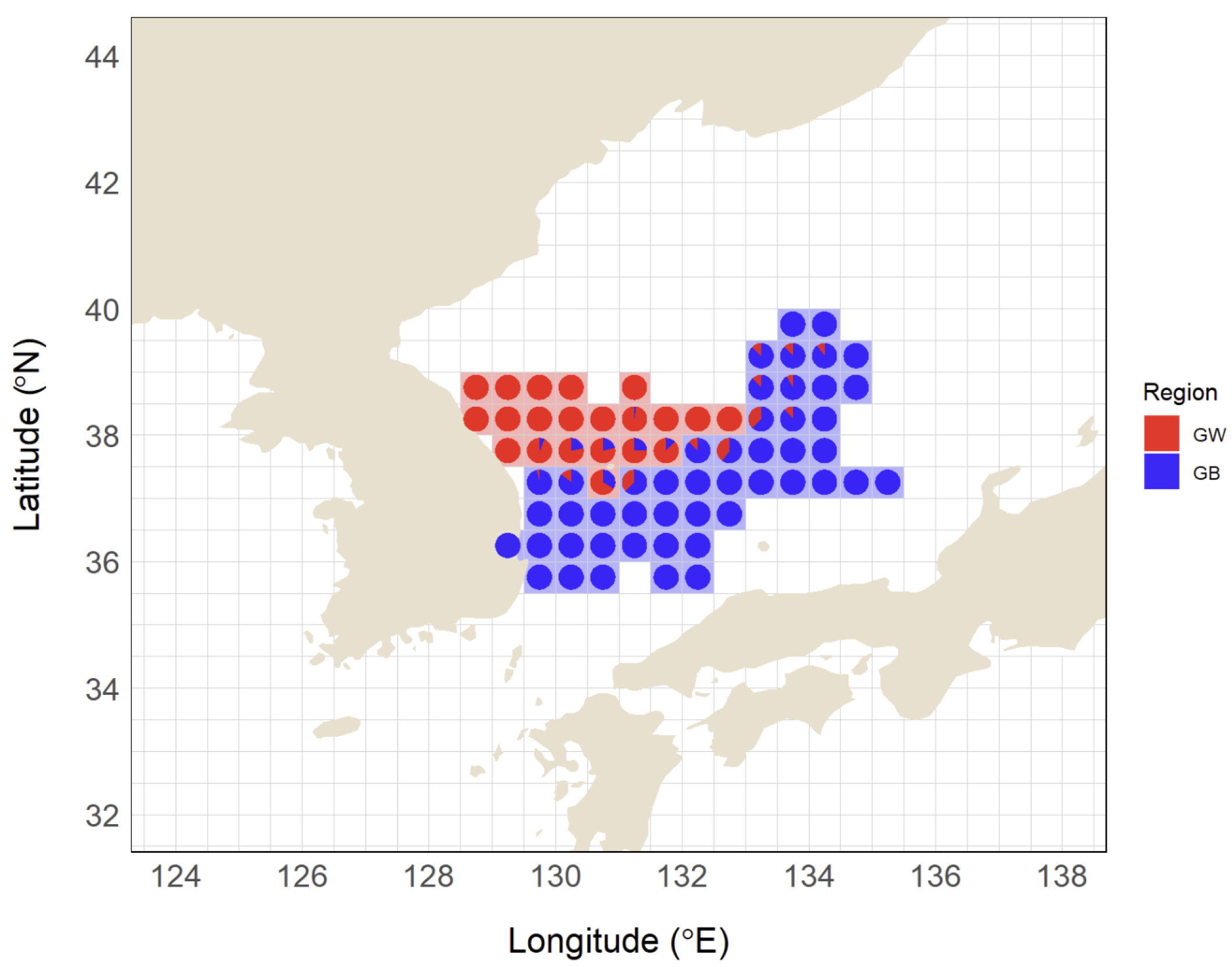
The red snow crab fishery in South Korea is primarily concentrated in the eastern coastal waters, with the two major fishing grounds located in the Gangwon (GW) and Gyeongbuk (GB) regions. These areas represent the core fishing zones for offshore trap fisheries targeting this species. The spatial distribution of the fishing effort is shown in
Figure 1, where fishing grids (0.5° × 0.5°) are color-coded to distinguish between the two regions. The classification of GW and GB fishing grounds was based on the fishing records of vessels registered in each respective region.
This allocation method ensures that the spatial representation accurately reflects the fishing effort distribution between the two regions. The total fishing area for each region was calculated using geospatial methods that account for the curvature of the Earth and the varying lengths of longitude at different latitudes. Based on these calculations, the estimated fishing area for GW was approximately 53,376 km2, while the GB region covered 115,898 km2. These estimates provide an essential basis for evaluating spatial differences in CPUE and understanding the regional allocation of fishing efforts.
2.2. Data and Variables
In this study, fishery-dependent CPUE data were obtained from official records reported by total allowable catch (TAC) surveyors in South Korea, covering the period from 2009 to 2023. These data include key operational variables such as total catch, live catch, fresh catch, fishing effort (number of trips), vessel size (gross tonnage), fishing date (year, month, and day), and fishing locations (latitude and longitude). As these records are based on regulated and systematic reporting, they provide a reliable basis for CPUE analysis.
To ensure the accuracy and consistency of the dataset, several preprocessing steps were conducted. First, records with incomplete information on catch, effort, or fishing location were removed, and outlier detection was applied using interquartile range (IQR) analysis to exclude anomalous CPUE values [
27]. Second, seasonal adjustments were made by excluding fishing operations conducted during the closed season (July–August) to prevent potential biases introduced by regulatory restrictions. Third, fishing areas were categorized into two regions, Gangwon (GW) and Gyeongbuk (GB), following the spatial classification applied in this study (
Figure 1). This classification allows for the differentiation of regional fishing efforts and spatial variations in CPUE while maintaining consistency with the defined study area. Additionally, vessel characteristics were classified into three categories based on gross tonnage: 8–20 tons, 20–40 tons, and over 40 tons, to account for variations in fishing efficiency.
In addition to fishery-dependent variables, socioeconomic factors were incorporated into the CPUE standardization model to account for external influences on CPUE. The socioeconomic variables considered in this study include COVID-19, live catch proportion, global export price, and oil price. The inclusion of socioeconomic variables enhances the robustness of CPUE standardization by distinguishing between changes in fishery-dependent CPUE that result from external economic pressures and those attributable to stock abundance fluctuations. By controlling for external drivers, the standardized CPUE more accurately reflects resource availability, improving the reliability of stock assessments and fisheries management decisions.
The COVID-19 pandemic had widespread effects on global fisheries, disrupting supply chains, reducing seafood demand, and altering fishing efforts due to movement restrictions and economic instability [
8,
28,
29]. In this study, COVID-19 was treated as a categorical variable with two levels: pre-pandemic (before 2020) and post-pandemic (2020 onward). The dataset was divided based on this temporal breakpoint to assess how CPUE patterns shifted due to pandemic-related market disruptions and operational constraints.
The proportion of live catch relative to the total catch reflects market demand dynamics and industry preferences [
30]. The inclusion of this variable in the model accounts for economic incentives that may influence fishing practices. For instance, an increasing preference for live crab sales could alter catch handling methods and affect CPUE estimates due to changes in discards or retention rates.
Global export price fluctuations can directly impact fishing efforts by influencing economic returns for fishers [
31,
32]. Data on global red snow crab export prices (USD per ton) were sourced from the national export records. Price trends determine the economic viability of fishing operations and can lead to variations in CPUE due to effort adjustments based on profitability. Higher export prices may incentivize increased effort, while declining prices may reduce fishing activity.
Fuel costs represent a significant portion of operational expenses for commercial fisheries [
33,
34,
35]. In this study, crude oil prices (USD per barrel) were used as a proxy for fuel costs and were obtained from publicly available energy market reports. Oil price volatility can impact fishing effort decisions, with higher fuel costs potentially leading to reduced fishing activity, shorter trips, or operational efficiency adjustments. This variable was included to capture economic constraints that might otherwise confound CPUE trends.
Table 1 provides a summary of the variables used in the CPUE standardization model. The fishery-dependent variables include temporal (year and month), spatial (fishing area and location), and vessel-specific (gross tonnage) factors that influence CPUE trends. The inclusion of spatial smoothing terms ensures that geographic differences in fishing efforts are adequately captured. In addition to these, socioeconomic variables were incorporated to account for external market and operational factors, such as the impact of the COVID-19 pandemic, fluctuations in global export prices, fuel costs, and shifting industry preferences for live versus fresh catch. These factors collectively enhance the robustness of the model by distinguishing stock availability-driven CPUE changes from those influenced by economic and regulatory conditions.
2.3. CPUE Standardization Model
CPUE standardization was performed using a generalized additive model (GAM), a flexible statistical approach that allows for non-linear relationships between CPUE and predictor variables. The response variable was the log-transformed CPUE, modeled as a function of multiple explanatory variables representing fishery–spatiotemporal and socioeconomic factors. The general form of the GAM used in this study is as follows:
where
denotes a smoothing function applied to continuous variables to capture non-linear relationships, and socioeconomic factors represent the combination of socioeconomic variables, including the impact of the COVID-19 pandemic (COVID), the proportion of live catch (LP), global export prices (GP), and oil prices (OP). The error term
follows a normal distribution.
Each of the explanatory variables incorporated in the model is detailed in
Table 1. The categorical variables such as Year, Month, Area, and GT were included to account for fishery–spatiotemporal variations in CPUE. In particular, we included Area (Gangwon and Gyeongbuk) to capture regional heterogeneity in fleet behavior and fishing strategies, which also contributes to reducing spatial dependence in model residuals.
Spatial variations in catch rates were further controlled by incorporating a two-dimensional smoothing function , which allows the model to flexibly capture spatial structure in the data. This term addresses potential spatial autocorrelation by modeling localized spatial patterns that might otherwise bias CPUE estimates. In addition to these fishery-dependent variables, socioeconomic factors were included to evaluate their influence on CPUE fluctuations over time.
To assess the impact of socioeconomic factors on CPUE standardization, six different GAM models were constructed, each incorporating a progressive set of explanatory variables (
Table 2). The base model (Model 1) accounts for fishery-spatiotemporal and vessel-related factors, including year, month, fishing area, gross tonnage, and spatial variability through a smoothing function for latitude and longitude. This model serves as a reference for evaluating the additional explanatory power of socioeconomic variables.
Model 2 extends the base model by introducing COVID-19 as a categorical variable, allowing the assessment of how pandemic-related disruptions influenced CPUE trends. Model 3 further includes live catch proportion as a smoothing term to capture economic incentives that may affect fishing behavior, such as the increasing preference for live crab sales. Model 4 builds upon Model 3 by incorporating global export prices, acknowledging the role of international market dynamics in shaping fishing efforts. Model 5 adds crude oil prices as an additional predictor, recognizing that fuel costs significantly influence vessel operations and fishing frequency. Finally, Model 6 refines Model 5 by incorporating an interaction term for live catch proportion by fishing region, allowing for regional differences in market demand and fleet behavior to be accounted for. This final model is expected to provide the most comprehensive representation of CPUE fluctuations by integrating both economic and spatial interactions.
To determine the optimal model for CPUE standardization, we compared six candidate GAM models (
Table 2) using a set of five performance metrics: Akaike Information Criterion (AIC), Bayesian Information Criterion (BIC), Mean Absolute Error (MAE), Root Mean Square Error (RMSE) and adjusted R-squared (R
2). These metrics were selected to provide a balanced assessment between model fit, complexity, and predictive accuracy.
The six models were constructed in a stepwise manner, beginning with fishery-dependent spatiotemporal variables (Model 1) and then progressively incorporating socioeconomic variables such as the COVID-19 pandemic (Model 2), live catch proportion (Model 3), export prices (Model 4), and oil prices (Model 5). Finally, Model 6 included a regional interaction term for live catch proportion to capture distinct fishing behaviors between Gangwon (GW) and Gyeongbuk (GB) regions.
This progressive modeling approach allowed us to assess the additive explanatory power of each variable and to evaluate whether their inclusion improved not only statistical performance but also the interpretability and realism of the model in the context of Korean red snow crab fisheries.
2.4. Analysis of Socioeconomic Influence and Year Effect
To assess the influence of socioeconomic factors on standardized CPUE, we conducted a stepwise exclusion analysis based on the final standardized model. In this approach, alternative predictions were generated by selectively omitting the effects of specific socioeconomic variables while maintaining the structure and coefficients of the final model.
The analysis proceeded in a stepwise manner: (a) the full standardized model including all predictors, (b) excluding the COVID-19 pandemic variable, (c) additionally removing international landings price (LP), (d) further excluding global production (GP), and (e) finally removing all socioeconomic variables, leaving only fishery-spatiotemporal factors in the model. Comparing the predicted CPUE values at each step enabled us to evaluate the relative contribution of each socioeconomic factor to interannual CPUE variability.
To further clarify the role of the year effect, we also produced predictions based solely on the categorical year variable, excluding all other factors. This allowed us to isolate the independent influence of interannual variation and better assess whether fluctuations in CPUE reflect changes in relative stock availability.
The results from the stepwise exclusion analysis, along with the year-effect-only predictions, were compared against observed CPUE, fully standardized CPUE, and standardized CPUE with all socioeconomic factors excluded. This provided a comprehensive understanding of the contribution of individual explanatory variables—particularly socioeconomic drivers—to CPUE trends and clarified the interpretability of the year effect as an indicator of relative abundance.
To facilitate comparisons across different models, the annual mean of the fitted CPUE values from each model variation was computed. The standardized CPUE trend for each year was estimated as
where
represents the standardized CPUE index for the
ith year,
is the number of observations in that year, and
corresponds to the
kth fitted CPUE value in the
ith year. This method ensures that annual fluctuations in CPUE are effectively captured while accounting for the impact of socioeconomic influences.
To standardize the comparison, all CPUE values were transformed into relative CPUE by normalizing against the mean CPUE across all years in the full model. This transformation allows for a direct assessment of changes in CPUE trends when specific socioeconomic factors are removed.
4. Discussion
We compared the year effects across six candidate models (
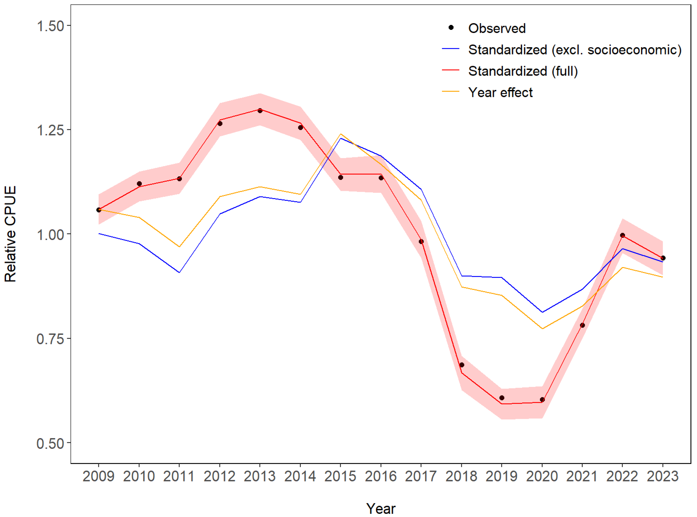
Figure 2). Notably, the year effect represents the standardized CPUE, which serves as an index of relative abundance after removing the effects of fishing operations and socioeconomic factors. The comparison shows that the nominal CPUE closely tracks the year effects in simpler models (e.g., Model 1 and Model 2), particularly in recent years. However, from 2016 to 2020, these unadjusted values deviate significantly from the year effects estimated in the final model (Model 6). This discrepancy highlights the influence of covariates such as vessel characteristics, regional catch dynamics, and economic factors (e.g., export price and oil price), which are only considered in the more complex models.
The comparison between the fully standardized CPUE and the standardized CPUE with all socioeconomic factors removed highlights the substantial influence of economic factors on CPUE variability. The fully standardized CPUE exhibited greater fluctuations over time, particularly from 2016 onward, whereas the CPUE without socioeconomic factors followed a smoother trajectory. This suggests that a significant portion of recent CPUE fluctuations may be driven by external market dynamics, economic conditions, and operational costs rather than changes in stock abundance alone. The relatively stable CPUE trend observed after removing socioeconomic influences indicates that these factors contributed to variability in observed CPUE rather than reflecting actual population fluctuations. These findings underscore the importance of incorporating socioeconomic variables in CPUE standardization to prevent fishing effort-related biases from distorting stock assessments. Without accounting for economic drivers, CPUE trends could be misinterpreted, potentially leading to suboptimal fisheries management decisions.
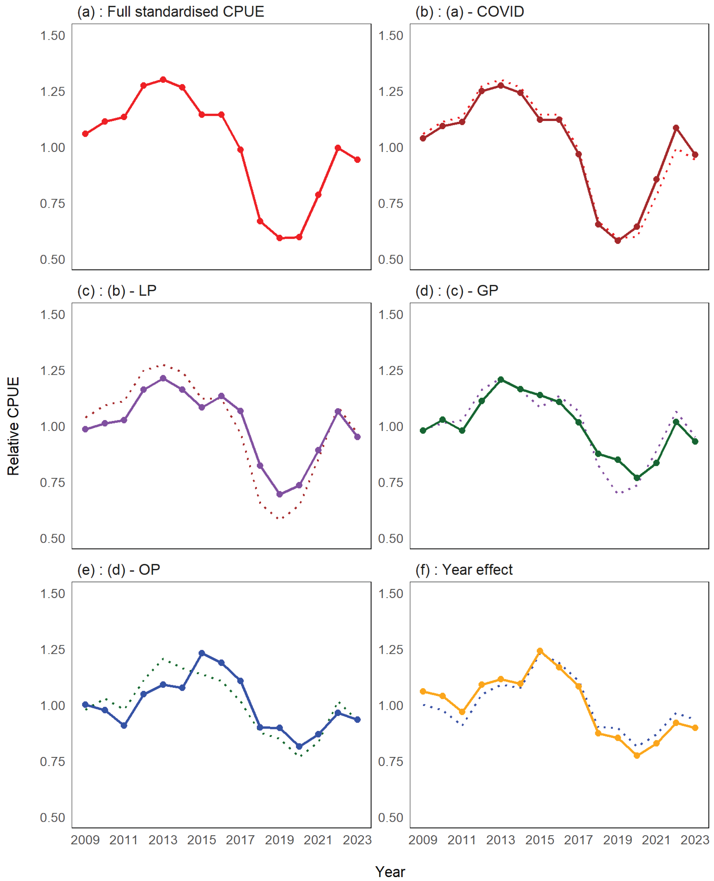
The stepwise exclusion analysis revealed that removing the COVID-19 variable (
Figure 4b) had a minimal effect on overall CPUE trends, though slight differences were observed in 2020–2021. The small increase in CPUE estimates during this period suggests that the pandemic may have had a suppressive effect on CPUE, possibly due to reduced fishing efforts, supply chain disruptions, and shifts in seafood market demand [
8,
28,
29]. However, the limited impact observed in this study could be attributed to the adaptability of the red snow crab fishery, which adjusted to pandemic-induced market changes by modifying fishing strategies and prioritizing higher-value products. During the pandemic, domestic demand and export volumes for fresh (processed) crab declined due to logistical challenges and reduced consumer demand. In response, the fishery shifted toward increasing live crab production, which commands a higher market price and is less affected by processing and distribution constraints. This strategic adjustment likely helped stabilize fishing efforts and mitigate the economic impact of COVID-19 on the industry.
The removal of the live catch proportion (LP) (
Figure 4c) led to a distinct upward shift in CPUE estimates around 2019. This suggests that variations in live catch proportions significantly influenced CPUE during this period. Vessels targeting live crabs require specialized onboard facilities such as water tanks to maintain survival, which limits their handling capacity compared to those processing fresh crabs. Consequently, even with the same fishing effort, the nominal CPUE for live crab vessels tends to be lower due to reduced storage capacity and handling constraints. The sharp increase in CPUE after excluding LP highlights its role in catchability and fleet behavior. Since live crabs command a higher market value [
30], fishers may adjust their fishing strategies, such as gear use and retention practices, to optimize profitability. By incorporating LP into the standardization process, CPUE estimates were adjusted upward, correcting for the artificially lower values recorded by live crab vessels. This adjustment ensures that CPUE trends reflect actual stock abundance rather than operational differences driven by economic incentives.
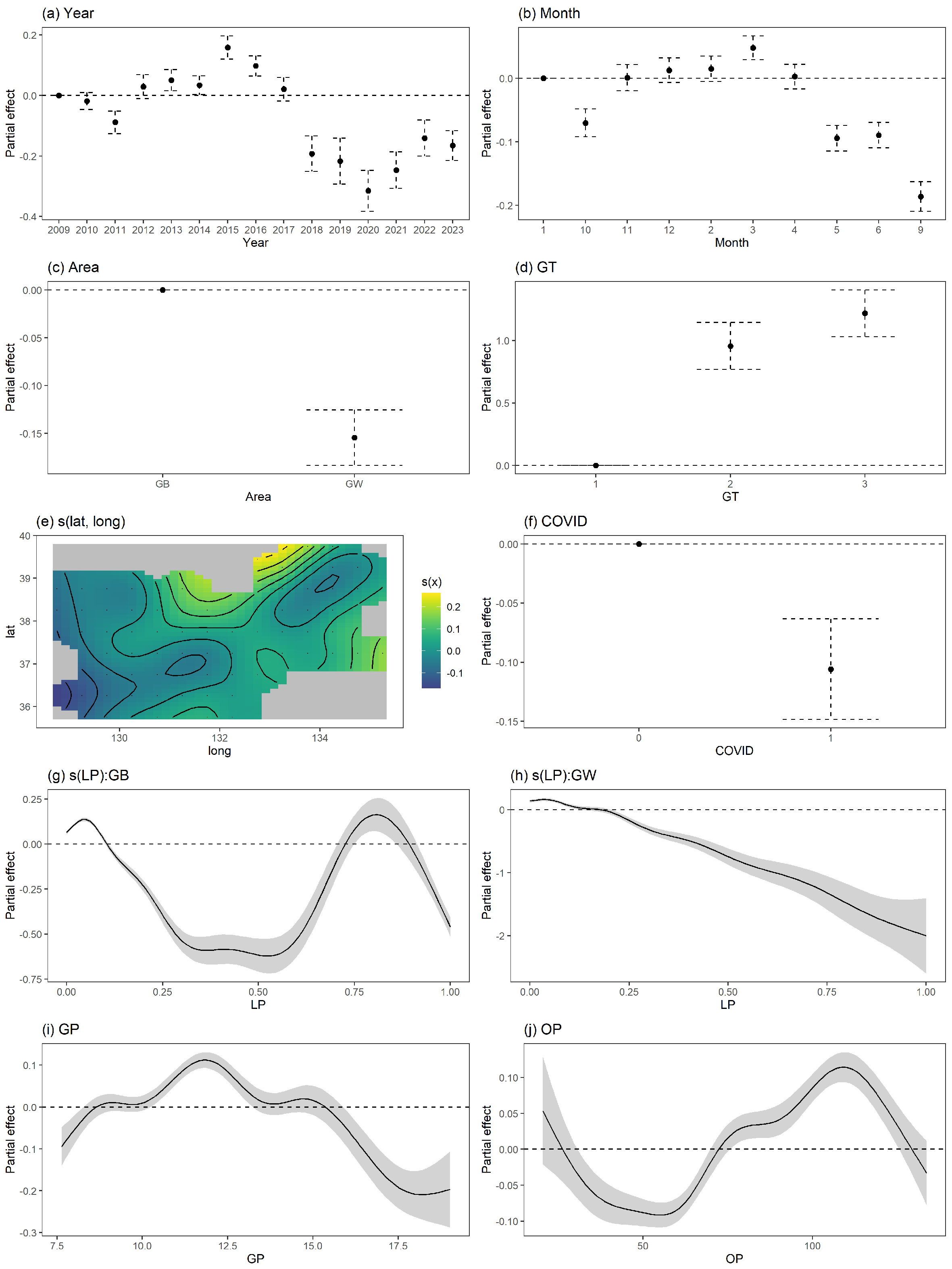
Furthermore, the partial effects of LP differed significantly between the two regions (
Figure 3g,h). In the GW region, the effect of LP on CPUE showed a consistent negative trend, suggesting that higher proportions of live catch are associated with reduced CPUE. This may be attributed to the operational limitations of live crab vessels, which generally have smaller storage capacity compared to vessels targeting processed or fresh crab, thus limiting the total amount of catch per trip.
In contrast, the GB region exhibited a non-linear response, with a local maximum in CPUE observed when the live catch proportion was around 0.75. This pattern could reflect the structural differences in the fleet composition. In GB, a greater number of vessels are equipped with larger water tanks and specialized facilities for live crab handling, enabling them to maintain higher catch volumes even with a high live catch ratio. As a result, the partial effect of live catch proportion in GB demonstrates a positive association with CPUE at higher values, in contrast to the trend observed in GW.
The exclusion of the global export price (GP) (
Figure 4d) resulted in greater deviations in CPUE in 2019, suggesting that international market conditions significantly influenced CPUE during these years. In
Figure 3i, the partial effect of GP on CPUE shows a non-linear trend. Specifically, CPUE increases as GP rises up to a value of approximately 12, suggesting that higher prices initially incentivize fishing activity due to improved profit margins. However, beyond this threshold, the partial effect declines. This pattern implies that when export prices become excessively high, international demand may decline due to price sensitivity, leading to a reduction in fishing efforts.
The next step in the exclusion analysis involved removing the oil price (OP) (
Figure 4e), resulting in a more stabilized CPUE trend with reduced interannual fluctuations. This indicates that fuel costs strongly influence fishing effort and CPUE variability [
33,
34,
35]. In
Figure 3j, At lower oil price levels, CPUE tends to rise, likely due to reduced operational costs that encourage more frequent or longer fishing trips. However, as oil prices increase beyond a certain point, CPUE declines, reflecting the economic burden placed on fishing operations. Interestingly, at very high OP levels, the effect appears to stabilize or slightly rebound, possibly indicating strategic adaptations by fishers—such as optimizing trip efficiency or targeting high-yield grounds—to offset rising fuel expenses.
In particular, during the period from 2009 to 2015, rising fuel costs prompted fishers to optimize their operations by targeting more efficient fishing grounds to maximize catch while minimizing fuel consumption. This shift is evident in the historical distribution of red snow crab fishing grounds, where the core fishing areas were concentrated closer to the shore during this period of high fuel prices [
18]. Since fishing effort in this study is measured in terms of trips rather than total fishing time or actual gear deployment, this operational adjustment resulted in fewer but more efficient fishing activities. Consequently, CPUE estimates appeared inflated, as fishers prioritized nearshore, more productive fishing locations while the recorded number of trips remained constant. This trend highlights how economic constraints, such as fuel price fluctuations, can influence spatial fishing behavior and, in turn, by incorporating oil price as a variable, these distortions were accounted for in the final standardized CPUE, leading to a more stable and realistic trend. This adjustment ensures that CPUE variations more accurately reflect stock abundance rather than economic constraints affecting fleet behavior.
This study’s approach is particularly effective in scenarios where scientific survey-based abundance indices are unavailable, and fishing effort data are limited. By integrating economic drivers, this method provides an alternative means of refining CPUE estimates and improving the accuracy of stock assessments. However, to further enhance confidence in these findings, future research should compare standardized CPUE trends derived from this method with abundance indices obtained from independent scientific surveys. Such comparisons would help validate the effectiveness of socioeconomic-adjusted CPUE estimates and strengthen their applicability in fisheries management.
Unlike pelagic species that are highly responsive to oceanographic changes [
43,
44,
45], deep-sea species are less sensitive to short-term variations [
46,
47] in sea surface temperature (SST) or primary productivity indicators like chlorophyll-
a. Red snow crab is primarily distributed at depths of 500–2000 m, where environmental conditions remain relatively stable, and it is known to inhabit waters with temperatures ranging between 0.1 and 0.3 °C [
48]. Given these habitat characteristics, this study did not incorporate oceanographic variables into the CPUE standardization process. The exclusion of environmental factors aligns with previous research indicating that deep-sea crustaceans are less influenced by SST variability compared to shallower-dwelling species. Instead, the focus was placed on socioeconomic drivers, which have been shown to significantly influence fleet behavior, fishing effort, and, ultimately, CPUE variability in economically driven fisheries.
These findings highlight the critical importance of interpreting the year effect within the context of a comprehensive model that incorporates relevant socioeconomic and operational variables. The year effect is commonly used as a proxy for changes in stock abundance. If standardization is performed without relevant variables, the resulting year effect may still contain considerable bias and fail to represent true changes in stock abundance. By incorporating variables such as fuel prices, export demand, and live catch preferences, the CPUE standardization process can more accurately isolate interannual abundance trends from external economic influences. This not only enhances the reliability of CPUE-based indices in data-limited fisheries but also supports more adaptive and evidence-based management strategies. Ultimately, minimizing confounding errors through the inclusion of socioeconomic drivers ensures that year effects more faithfully represent stock dynamics and provides a practical foundation for sustainable fisheries governance.
5. Conclusions
This study highlights the critical role of socioeconomic factors in CPUE standardization for red snow crab (Chionoecetes japonicus) fisheries. By incorporating variables such as fuel prices, export demand, and live catch preferences, this study enhances the accuracy of CPUE estimates, particularly in fisheries where scientific survey-based abundance indices are unavailable. The stepwise exclusion analysis demonstrated that these economic factors significantly influence CPUE trends, with their removal leading to a more stable trajectory, suggesting that external market conditions, rather than biological fluctuations, contribute to observed CPUE variability.
The findings underscore the importance of integrating economic considerations into stock assessments and fisheries management. Without accounting for these external influences, CPUE-based abundance estimates could be misinterpreted, potentially leading to ineffective management measures. This study’s approach provides a practical framework for improving CPUE standardization in data-limited fisheries, offering a more reliable assessment of stock status.
Future research should focus on validating these findings by comparing standardized CPUE trends with independent scientific survey-based abundance indices. Additionally, incorporating climate-related variables, particularly for long-term assessments, could further refine CPUE standardization models. The methodology developed in this study has broader applicability for other crustacean fisheries where market-driven economic shifts affect fishing efforts and CPUE trends. By integrating socioeconomic variables into fisheries assessments, management strategies can be more adaptive, ensuring the sustainability of red snow crab and similar fisheries in an evolving economic and environmental landscape.


