Abstract
Due to external environmental factors, the layout of compound channels in estuarine ports is restricted. Moreover, with the opposing distribution of anchorages and terminals within the port, vessels navigating between these areas must cross the channel, severely affecting channel navigation safety and efficiency. In order to improve the efficiency of vessel scheduling, we analyze the layout characteristics of an estuarine port and its compound channel, summarize vessel navigation modes and traffic flow conflicts, and identify five key conflict areas. On this basis, we develop a multi-objective optimization model aimed at minimizing vessel waiting times and the total channel occupancy time ratio. This model incorporates constraints such as navigation rules, traffic flow conflicts, tidal effects, and traffic control. To solve the model, we propose an adaptive non-dominated sorting genetic algorithm, ANSGA-NS-SA, which integrates neighborhood search (NS) and Simulated Annealing (SA). The entropy-weighted technique for order preference by similarity to ideal solution (TOPSIS) is used to calculate the objective weights of the Pareto frontier and identify the optimal solution. Experimental results show that the proposed model and algorithm yield optimal port entry and exit scheduling solutions. In terms of port scheduling performance, the proposed model and algorithm outperform the traditional First-Come-First-Served (FCFS) strategy and the Non-Dominated Sorting Genetic Algorithm II (NSGA-II), reducing total vessel waiting time by 33.8% and improving total channel occupancy ratio by 8.8%. This study provides a practical and effective decision support tool for estuarine port scheduling, enhancing overall port operational efficiency.
1. Introduction
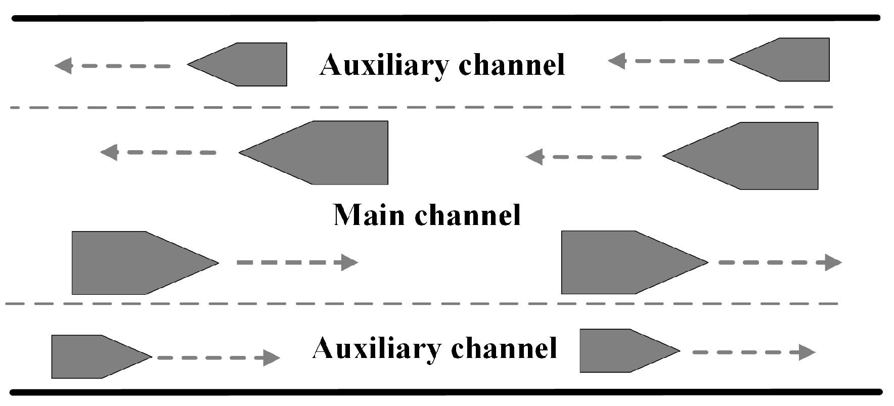
Maritime transport is the most critical mode of transportation for global trade, with over 80% of global trade volume moved by sea. According to the United Nations Conference on Trade and Development (UNCTAD), global maritime trade grew by 2.4% in 2023. The industry is projected to grow by an additional 2% in 2024 [1]. As the size and number of vessels increase, many ports face significant limitations in navigational capacity due to restricted channel throughput, leading to evident capacity shortfalls in port channels. To improve port service levels, many port channels have started widening projects and implemented virtual buoys to form compound channels [2]. As shown in Figure 1, large vessels navigate the main channel, while smaller vessels use the auxiliary channel on its outer side to reduce interference with larger vessels. Estuarine ports are located at the confluence of rivers and the sea, situated on tidal-sensitive river segments. As an important hub connecting inland waterways, coastal ports, and coastal channels, the navigational capacity of estuarine port channels is significantly constrained by insufficient channel width. To effectively address this issue, transforming estuarine port channels into composite channels has become a feasible and efficient solution. For instance, the deep-water channel of the Yangtze River estuary was successfully integrated with slope channels through the implementation of natural slope depth engineering. This integration led to the construction of the Yangtze River estuary compound channel, which significantly improved navigational efficiency. However, it is important to note that estuarine port compound channels differ considerably from seaport compound channels in terms of structure and environmental conditions. Seaport compound channels typically feature deep water and wide channels, whereas estuarine port compound channels are often narrower, with more variable conditions such as water flow and depth. Therefore, the design of estuarine port channels is often continuously adjusted based on the natural conditions of the waterways [3]. Due to the characteristics of inland ports, some estuarine ports exhibit a phenomenon where anchorages and terminals are oppositely distributed on both sides of the channel [4,5]. When barges travel between these opposing terminals and anchorages, they need to cross the channel, increasing the risk of collisions with vessels navigating through the channel. As the channel’s navigational capacity improves, this risk becomes more pronounced. In addition, some sections of estuarine port channels are narrow and restricted. Tidal variations can increase traffic flow density in these areas. When large vessels navigate through these restricted channels, it may lead to navigational safety issues, such as vessel yawing [6].

Figure 1.
Compound channel structure.
In the current vessel-scheduling scheme at estuarine ports, the port dispatch center arranges the schedule based on the order of arrival and departure times declared in advance by shipping companies. This scheduling method is known as the First-Come-First-Served (FCFS) strategy. The advantage of this strategy is that no models need to be established, making it simple and convenient. However, it may lead to excessive waiting times, reducing the efficiency of vessel entry and exit. This not only decreases the satisfaction of shipping companies with port services but could also have a negative impact on the long-term interests of the port. Shipping companies usually aim to reduce waiting times to save fuel costs, while port dispatch centers focus on shortening overall scheduling time and enhancing channel utilization by adjusting the order of vessel arrivals and departures. However, a conflict arises between the two, as altering the scheduling order may increase waiting times for certain vessels, thereby raising fuel costs [7]. Therefore, how to reasonably arrange ship scheduling to ensure navigational safety and improve port operational efficiency has become an urgent issue.
To address the above challenges, this study investigates the vessel-scheduling problem in an estuarine port with compound channels, considering the opposing distribution of inner anchorages and terminals. A vessel-scheduling model adapted to the compound channel of an estuarine port is established. An adaptive multi-objective genetic algorithm (ANSGA-NS-SA) is designed to solve the model, ultimately obtaining the optimal scheduling solution. The main contributions of this paper are as follows:
- (1)
- Based on a thorough analysis of an estuarine port, we propose the overall structural layout of the compound channels. We then analyze the vessel navigation mode and traffic flow conversion method within the channels and then identify key traffic conflict areas. This lays the foundation for subsequent vessel-scheduling optimization.
- (2)
- This study proposes a vessel-scheduling model for estuarine port compound channels, considering the opposing distribution of anchorages and terminals. The optimization model integrates practical constraints, including navigational safety, traffic flow conflicts, berth coordination, tidal influences, and traffic control. To balance the interests of port management and shipping companies, we set the minimization of total vessel waiting time and the ratio of total channel occupancy time as the optimization objectives. The model aims to enhance port scheduling efficiency while ensuring navigational safety.
- (3)
- To address the sensitivity of parameter selection and the risk of falling into local optima in the NSGA-II algorithm, this paper proposes a novel ANSGA-NS-SA algorithm. Numerical experiments are conducted on different problem sizes, where the ANSGA-NS-SA algorithm, the FCFS strategy, and the NSGA-II algorithm are used to solve the model. The results show that ANSGA-NS-SA consistently outperforms the other methods in both small- and large-scale instances. Moreover, sensitivity analysis indicates that ANSGA-NS-SA provides greater solution stability than the other two approaches.
The remainder of this paper is organized as follows. Section 2 reviews the relevant literature in the field of vessel scheduling. Section 3 provides a detailed analysis of vessel navigation modes and traffic conflict characteristics in the estuarine port channels. Section 4 develops a mathematical optimization model based on the physical layout of the estuarine port and relevant constraints. Section 5 describes the ANSGA-NS-SA algorithm for solving the model. Section 6 presents a case study and discusses the validity of the proposed model and the effectiveness of the algorithm. Finally, Section 7 concludes the paper and outlines directions for future research.
2. Related Work
In this section, we summarize the relevant research in the field of port channel vessel scheduling, as shown in Table 1. We have conducted a detailed analysis and comparison of the different studies based on aspects such as research problem attributes, channel types, constraints, objective functions, and methods used.
Existing studies mainly focus on the optimization of vessel scheduling under different types of channels and have established various vessel-scheduling optimization models. Liang et al. [8] studied vessel traffic scheduling in the controlled channels of the upper Yangtze River. They ranked the factors affecting vessel traffic and used an expert system to generate appropriate traffic commands, enabling the conversion of one-way traffic flow. Gan et al. [9] proposed a sliding-window online sorting and scheduling model for vessel scheduling in one-way restricted channels. By decomposing the problem, this model reduces computational complexity and significantly improves scheduling efficiency. Zhen et al. [10] optimized vessel scheduling in one-way channels using reinforcement learning, improving port operational efficiency by reducing waiting times and delays. Zhang et al. [11] studied vessel scheduling in one-way tidal channels, focusing on the impact of tidal depth. They established a mathematical model with the objective of minimizing total waiting time. Later, Zhang et al. [12] extended their research to two-way tidal channels, aiming to minimize total waiting time. They developed a vessel-scheduling model for two-way tidal channels affected by tides and solved it using a genetic algorithm. Zhao et al. [13] investigated real-time barge scheduling in river-sea channels. They designed a variable neighborhood search (VNS) algorithm to schedule barges within tidal windows, preventing barges from missing the tidal window. Zheng et al. [14] considered the practical constraints of two-way channels and safety regulations for nighttime navigation. They established a mixed-integer programming model aimed at minimizing total waiting time for vessels and designed a branch-and-cut algorithm with an embedded aggregation strategy to solve the model. Considering the impact of vessel speed on scheduling, Liu et al. [15] proposed a vessel-scheduling model with fuzzy speed to address the uncertainty in transportation time caused by variable speeds when vessels navigate through bidirectional channels. Later, Liu et al. [16] developed a scheduling model aiming to reduce the average waiting time for consecutive vessel-scheduling problems considering uncertain sailing speeds and solved it using a genetic algorithm. Jiang et al. [17] addressed the vessel-scheduling problem in restricted channels with resource constraints, proposing a mathematical model that incorporates complex channel rules and scheduling resource constraints, with the objective of minimizing the total waiting time of vessels, and solved it using an elitist selection genetic algorithm. Jiang et al. [18,19] developed a comprehensive scheduling model for vessels in restricted channels with multi-resource integration considering factors such as tidal times, traffic conflicts, and carbon emissions and designed a multi-objective optimization algorithm to effectively reduce vessel delays and carbon emissions. Zhang et al. [20] constructed a physical model for the compound channel of Tianjin Port considering constraints such as tidal time and safety time and proposed a multi-objective vessel traffic scheduling optimization model. Jia et al. [21] based their work on the physical layout of Shanghai Waigaoqiao Port, establishing a compound channel vessel-scheduling model to minimize total costs, incorporating pilot scheduling decisions, and designed a Lagrange relaxation algorithm to solve it.
However, the studies mentioned above rarely involve incorporating port facilities such as terminals and anchorages into vessel-scheduling optimization models. As port facilities become more complex, some studies have started to explore the inclusion of these factors in channel scheduling models. Jia et al. [22] investigated the setup of an inner anchorage buffer zone in port basin waters and established a mixed linear mathematical model to optimize channel traffic and anchorage utilization, with berth, tides, navigation rules, and anchorage capacity as constraints. Li et al. [23] focused on vessel scheduling in restricted channels shared by multiple port basins. They proposed a multi-objective optimization model that considers tidal times, traffic conflicts, carbon emissions, and other factors, and solved it using an algorithm combining NSGA-II and Tabu search, significantly improving vessel transit efficiency. Jia et al. [24] analyzed a passenger roll-on/roll-off terminal with a restricted turning basin and constructed a vessel-scheduling model for coordinating the turning basin and channel. However, these studies primarily focus on seaport environments and treat port facilities like anchorages as constraints in the scheduling process without analyzing how the layout of these facilities alters vessel operational patterns. Regarding the research on the impact of anchorages and berths on navigation, Wang et al. [25] developed a simulation model for the composite system of ports, channels, and anchorages, analyzing the effect of different numbers of anchorages on vessel navigation rules. Liao et al. [26] also built a simulation model to assess the impact of reallocating anchorage plans on the operation of large ports. However, these methods are based on simulation systems and discuss the impact of anchorage and berth configurations on overall scheduling outcomes. There is a lack of studies using mathematical models to precisely describe the impact of anchorage and berth distribution on vessel traffic.
After the above analysis and based on the content in Table 1, it is found that there is extensive research on one-way, two-way, and restricted channels, but relatively less on compound channels. According to the literature we have reviewed, research on compound channels mainly focuses on Tianjin Port, which is a sea port compound channel. There is a lack of studies on the application of compound channels in estuarine ports. Estuarine ports, located at the junction of inland waterways and maritime channels, have significant differences in their external environment compared to sea port channels. These differences include the distribution of inland anchorages and the structure of the channels. When the channels are transformed into compound channels, the distribution of anchorages and terminals in the river may lead to changes in vessel operating patterns. Therefore, previous models and methods cannot fully apply to vessel scheduling in estuarine port compound channels.

Table 1.
Literature review.
Table 1.
Literature review.
| Reference | Problem Attributes | Channel Type | Constraint | Objective Function | Solution Method | ||||||||||||
|---|---|---|---|---|---|---|---|---|---|---|---|---|---|---|---|---|---|
| Inland Rivers | Port | 1 | 2 | 3 | 4 | 5 | 6 | 7 | 8 | 9 | 10 | 11 | 12 | ||||
| [8] 2019. | √ | one-way | √ | √ | 1 | S | |||||||||||
| [9] 2021. | √ | one-way | √ | √ | √ | √ | √ | √ | 1 | SWA | |||||||
| [10] 2025. | √ | one-way | √ | √ | √ | √ | 1 + 7 | RL | |||||||||
| [11] 2020. | √ | one-way | √ | √ | 1 | GA | |||||||||||
| [22] 2019. | √ | two-way | √ | √ | √ | √ | √ | √ | √ | √ | √ | 4 | LR | ||||
| [12] 2020. | √ | two-way | √ | √ | √ | √ | √ | 1 | GA | ||||||||
| [13] 2023. | √ | two-way | √ | √ | √ | √ | √ | 2 | VNS | ||||||||
| [14] 2021. | √ | two-way | √ | √ | √ | 1 | BC | ||||||||||
| [15] 2021. | √ | two-way | √ | √ | √ | √ | 5 | FS + GA | |||||||||
| [16] 2021. | √ | two-way | √ | √ | √ | √ | √ | √ | 3 | GA | |||||||
| [23] 2021. | √ | restricted | √ | √ | √ | √ | √ | √ | √ | 1 + 2 | MOGA + TS | ||||||
| [17] 2023. | √ | restricted | √ | √ | √ | √ | √ | √ | 1 | GA | |||||||
| [18] 2022, [19] 2024. | √ | restricted | √ | √ | √ | √ | √ | √ | √ | √ | √ | √ | 1 + 6 | MOGA | |||
| [24] 2023. | √ | restricted | √ | √ | √ | √ | √ | 1 + 2 | ACO | ||||||||
| [20] 2019. | √ | compound | √ | √ | √ | √ | √ | √ | √ | √ | 1 + 6 | MOGA | |||||
| [21] 2020. | √ | compound | √ | √ | √ | √ | √ | 4 | LR | ||||||||
| Our work | √ | compound | √ | √ | √ | √ | √ | √ | √ | √ | √ | √ | 1 + 8 | MOGA + NS + SA | |||
Constraints = {1: Safety interval distance/time, 2: Tidal time, 3: Speed, 4: Vessel priority, 5: Traffic conflict, 6: Multiple channel entrance, 7: Navigation prohibition period, 8: Berth, 9: Inner anchorage, 10: Traffic flow conversion, 11: Traffic flow coordination, 12: Tugboat}. Objective functions = {1: Minimize the total waiting time, 2: Minimize total scheduling time, 3: Minimize average wait time, 4: Minimize the total cost, 5: Minimize maximum completion time, 6: Minimizing total carbon emissions, 7: Minimize delays, 8: Minimize channel occupancy time ratio}. Solution methods = {S: Simulation study, SA: Simulated annealing algorithm, SHA: Self-built heuristic algorithm, FS: Fuzzy scheduling model, LR: Lagrange relaxation, BC: Branch-cut algorithm, GA: Genetic algorithm, RL: Reinforcement learning, SWA: Sliding-window algorithm, MOGA: Multi-objective genetic algorithm, TS: Tabu search, VNS: Variable neighborhood search, NS: Neighborhood search}.
3. Characteristics of Compound Channels in Estuarine Port
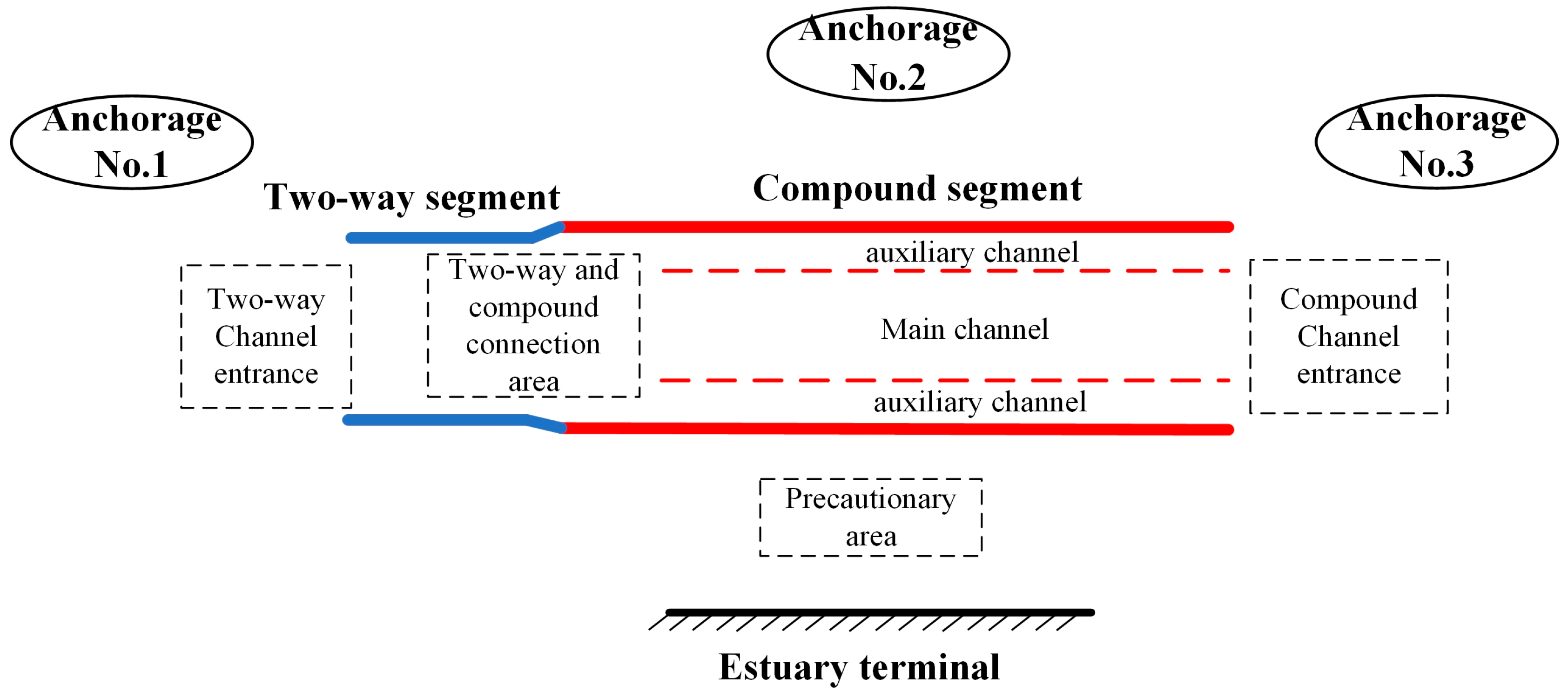
In this section, we construct a port layout model based on Taicang Port, an estuarine port along the Yangtze River estuary. The model includes channels, anchorages, and terminals, as shown in Figure 2. The channel is a combination of a two-way channel and a compound channel, with entrances at both ends for the compound and two-way channels. Three inner anchorages are located in the northern part of the channel, while the terminals are situated on the southern side. Figure 3 presents a schematic diagram of vessel entry and departure. As shown in the figure, vessels entering the terminal arrive from both the two-way channel entrance and the compound channel entrance. Additionally, some vessels cross the channel directly to carry out berthing and unberthing operations. When vessels cross between the anchorages and terminals, they significantly interfere with vessels navigating within the compound channel, complicating vessel encounters.
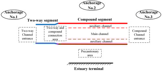
Figure 2.
Layout of estuarine port and channel.
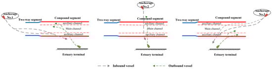
Figure 3.
Schematic diagram of vessel entry and departure.
3.1. Navigation Modes of Vessels in Channels
The channel consists of a two-way segment and a compound channel segment. In the two-way segment, vessels can navigate in either two-way or one-way mode. In the compound channel segment, vessels in the auxiliary channel must navigate in one-way mode, while vessels in the main channel can navigate in either two-way or one-way mode. Therefore, there are three types of navigation modes in the channel: one-way navigation, two-way navigation, and mixed one-way and two-way navigation. One-way and two-way navigation refer to vessels maintaining a consistent mode throughout the entire channel. When vessels navigate to the connecting area between the two-way and compound channel segments, they need to change their navigation mode to mixed one-way and two-way navigation. According to port channel regulations, vessels with a length or breadth below the minimum threshold must navigate two-way in the two-way channel segment and one-way in the auxiliary channel of the compound segment. Vessels within a specified intermediate range of length or breadth maintain two-way navigation in both the two-way channel segment and the main channel of the compound segment. Vessels exceeding the maximum threshold must adopt one-way navigation in both the two-way channel segment and the main channel of the compound segment.
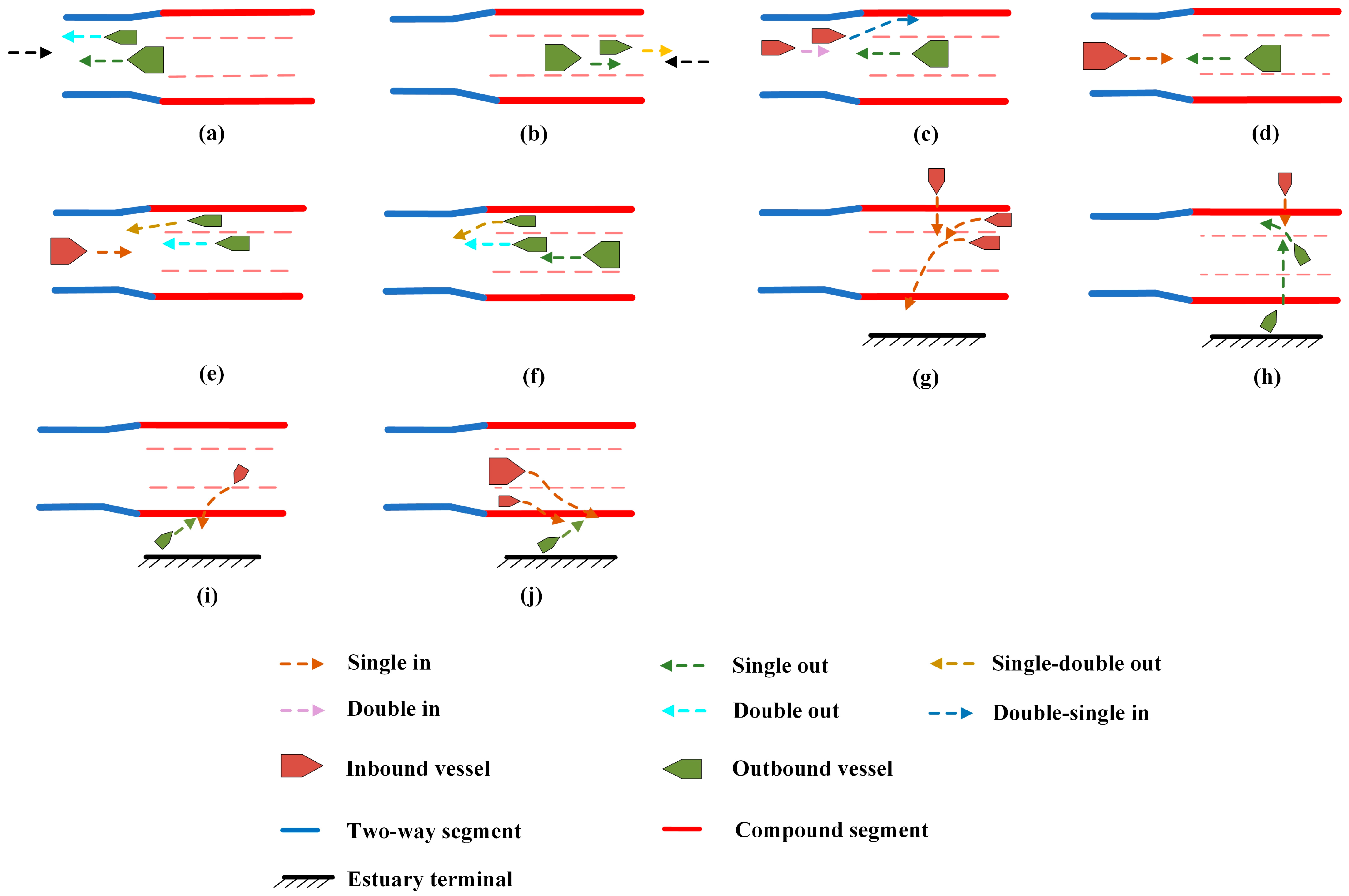
Based on vessel navigation modes, vessel traffic flow in the channel can be categorized into one-way, two-way, or mixed one-way and two-way traffic flow. When the traffic flow is one-way, it is defined as single in or single out. In the case of two-way traffic flow, it is defined as double in or double out. For mixed one-way and two-way traffic flow, it is defined as double-single in or single-double out. Six types of vessel traffic flow exist in the channel, as shown in Figure 4a–f. When a constant type of traffic flow is in operation, overtaking within the channel should be avoided. Figure 4g,h illustrate the scenario when vessels cross the channel to enter or depart from anchorage no. 2 and the terminals. According to port channel regulations, only one vessel is allowed to cross at a time, and vessels crossing must yield to those navigating normally in the compound channel. Moreover, during peak traffic periods, the maritime command center enforces traffic control measures that prohibit crossings.
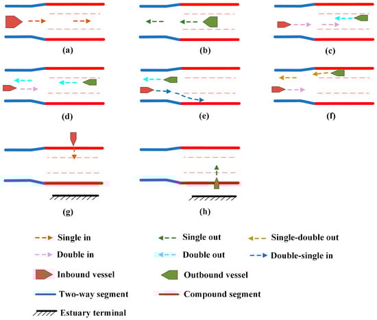
Figure 4.
(a–f) illustrate six types of vessel traffic flow in the channel, while (g,h) depict vessel crossing scenarios.
3.2. Vessel Traffic Conflict Characteristics
In this subsection, we analyze the characteristics of vessel traffic conflicts in the channel based on traffic flow. Vessel conflicts in the channel mainly include three types: overtaking, head-on collisions, and crossing collisions. As shown in Figure 5a,b, at the entrances of the two-way and compound channels, when the vessel traffic flow is one-way or two-way, head-on collisions occur with inbound vessels. At the connection area between the two-way and compound channels, head-on collisions also occur between inbound and outbound vessels when the inbound traffic is one-way, two-way, or mixed navigation modes (Figure 5c–e). Additionally, within the compound channel segment, outbound vessels from the main and auxiliary channels converge at the connection area, leading to overtaking conflicts (Figure 5f). At the entrance where vessels cross the channel, those preparing to cross may experience crossing collisions with other inbound vessels (Figure 5g) or even head-on collisions with outbound vessels crossing the channel (Figure 5h). In the precautionary area between the terminals and the channel, inbound vessels leave the channel to proceed toward the berths, while outbound vessels enter the channel (Figure 5i,j). Due to the limited space in the precautionary area, head-on traffic conflicts may occur between inbound and outbound vessels.
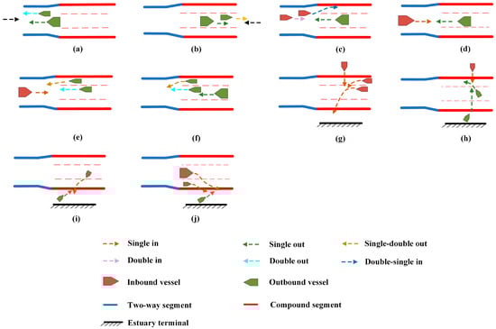
Figure 5.
Vessel traffic conflicts: (a,b) represent conflicts at the entrances of the two-way and compound channels; (c–f) represent conflicts at the connection of the two-way and compound channels; (g,h) represent entrance conflicts when vessels cross the channel; (i,j) represent conflicts in the precautionary area.
4. Problem Description and Optimization Model
4.1. Problem Description
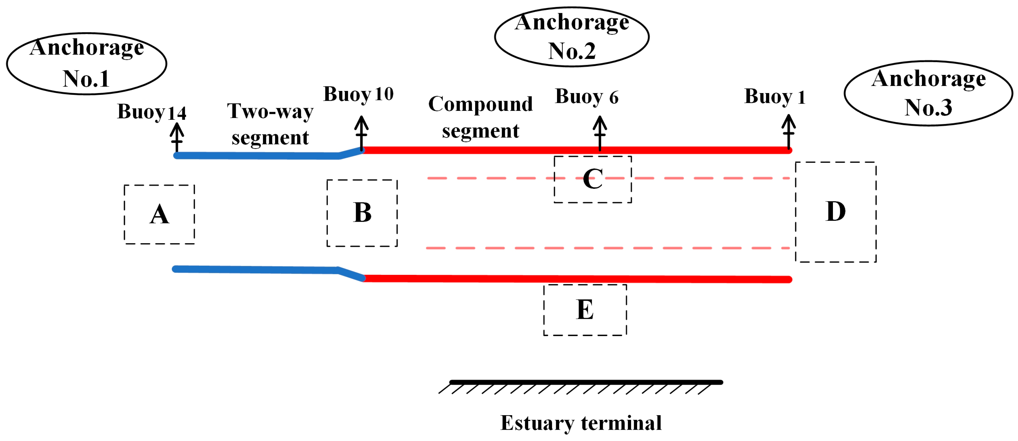
Based on the content of Section 3, the general structure of the estuarine port is abstracted to include anchorages, channels, and terminal berth areas. As shown in Figure 6, inbound vessels at anchorage no. 1 enter via Buoy 14, while those at anchorage no. 3 enter via Buoy 1. Inbound vessels that cross the channel berth at anchorage no. 2, with the crossing entrance located at Buoy 6. Buoy 10 is located in the connect area between the two-way channel segment and the compound channel segment, where the channel narrows sharply at a sharp turning point. To avoid collision risks during turns, head-on encounters should be avoided in this area. Key conflict areas within the channel have been abstracted and labeled as follows: the entrance of the two-way channel is marked as area A; the connection between the two-way and compound channel segments is marked as area B; the entrance for vessels crossing the channel is marked as area C; the entrance of the compound channel is marked as area D; and the precautionary area is marked as area E. To ensure the safety of vessel navigation and the efficiency of scheduling in the estuarine port, the following assumptions are made for the mixed-integer programming model:
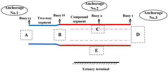
Figure 6.
Key areas of vessel conflict in estuary harbor channels.
- (1)
- The scheduling start and end nodes for inbound vessels are defined as from the anchorage to the berth, while the scheduling start and end nodes for outbound vessels are defined as from the berth to the channel exit.
- (2)
- The influence of tugboats and pilots is not considered, assuming there are sufficient tugboats and pilots available.
- (3)
- Berths are treated as discrete units, with predetermined berths for inbound vessels, and specific berth assignments are not considered.
- (4)
- Factors such as weather conditions, obstructions, and vessel malfunctions during navigation are not taken into account.
4.2. Optimization Model
The entire planning period is discretized for representation, and the notation used in the model is summarized in Table A1 of Appendix A.
Objective function:
Equation (1) represents the minimization of the total waiting time of vessels; Equation (2) represents the minimization of the total channel occupancy time ratio, which is used to measure the channel utilization within the scheduling scheme. These two objectives are potentially conflicting. Objective 1 aims to reduce the waiting time for vessels entering and leaving the port, which typically requires optimizing vessel scheduling. This would encourage vessels to enter the channel and berth as quickly as possible, thus improving operational efficiency. However, reducing waiting time may allow more vessels to enter the channel simultaneously, leading to longer transit times through congested areas and ultimately increasing channel occupancy time.
Start scheduling time constraint:
Constraint (3) is used to adjust the application scheduling time for tidal vessels and vessels subject to traffic control, ensuring that vessels requiring tidal navigation can enter the channel within the tidal window, and vessels under traffic control do not operate during the control period. Constraint (4) represents the start scheduling time of the vessel
Navigation time constraints:
Constraints (6) and (7) calculate the times when vessels departing from anchorage no. 1 reach various areas of the channel. Constraint (8) represents the time when vessels departing from anchorage no. 2 cross the channel. Constraints (9) and (10) represent the times when vessels departing from anchorage no. 3 reach various areas of the channel. Constraint (11) represents the time when inbound vessels arrive at the berth after leaving the channel. Constraints (12) to (16) represent the times when outbound vessels reach various areas of the channel.
Safety interval constraints:
Constraints (17) and (18) represent the minimum safety time intervals required for vessels under different conditions, where parameter m is the safety distance coefficient. Constraint (17) represents the minimum safety time interval that must be maintained between vessels moving in the same direction, while Constraint (18) represents the minimum safety time interval that must be maintained between vessels moving in opposite directions.
Traffic flow conflicts constraints:
Areas A and D are located at the channel’s endpoints. Vessels in these areas follow similar constraints. Constraints (19) to (23) define the slot allocation sub-model for these areas. Constraint (19) prohibits overtaking between vessels moving in the same direction when entering these areas. Constraints (20) to (22) ensure that when outbound vessel and inbound vessel meet head-on in area A or D, they maintain a minimum opposite-direction safety interval. Constraint (23) ensures this minimum interval when outbound and inbound vessels navigate in a two-way mode and face head-on in area A.
Constraints (24) to (27) form the traffic coordination sub-model for area B. Constraints (24) and (25) ensure that, when outbound vessels from the main and auxiliary channels of the compound channel converge in area B, outbound vessels in the main channel have priority over those in the auxiliary channel to enter the two-way channel segment, maintaining a minimum same-direction safety interval. Constraint (26) represents the minimum opposite-direction safety interval required for inbound vessel to yield to outbound vessel in area B. This applies when both vessels are operating in one-way navigation or when one vessel is in two-way navigation. Constraint (27) represents the minimum opposite-direction safety interval that must be maintained between outbound vessel and inbound vessel when the navigation mode in area B changes, such as when vessels operate in a mixed one-way and two-way mode.
Constraints (28) to (32) form the vessel conflict coordination sub-model in area C. Constraint (28) represents the minimum same-direction safety interval that must be maintained between inbound vessels in the same direction in area C. Constraints (29) and (30) represent the minimum safety interval required for inbound vessel from anchorage no. 2 to yield to inbound vessel from anchorage no. 3 when they converge in area C. Constraint (31) represents the minimum safety interval that must be maintained between outbound vessel and inbound vessel , both navigating in one-way mode in area C. Constraint (32) represents that in area C, outbound vessel , when navigating in one-way mode, must yield to inbound vessel navigating on the main channel of the compound channel.
Constraints (33) to (36) form the vessel conflict coordination resolution sub-model for area E. Constraint (33) ensures that at any given time, at most one outbound vessel from different terminals has navigated to area E. Constraint (34) ensures that the inbound vessel and the outbound vessel , allocated to the same terminal, maintain a safe navigation interval in area E. Constraint (35) ensures that the inbound vessel and the outbound vessel , allocated to different terminals, maintain a safe navigation interval in area E. Constraint (36) ensures that the departure time of an outbound vessel is earlier than the arrival time of an inbound vessel at area E when allocated to the same berth.
Constraint (37) determines whether the navigation directions of the two vessels are the same. Constraint (38) defines the navigation mode of the vessels based on port regulations.
Finally, Constraint (39) represents 0-1 decision variables. Constraint (40) represents an integer decision variable.
5. Solution Approach
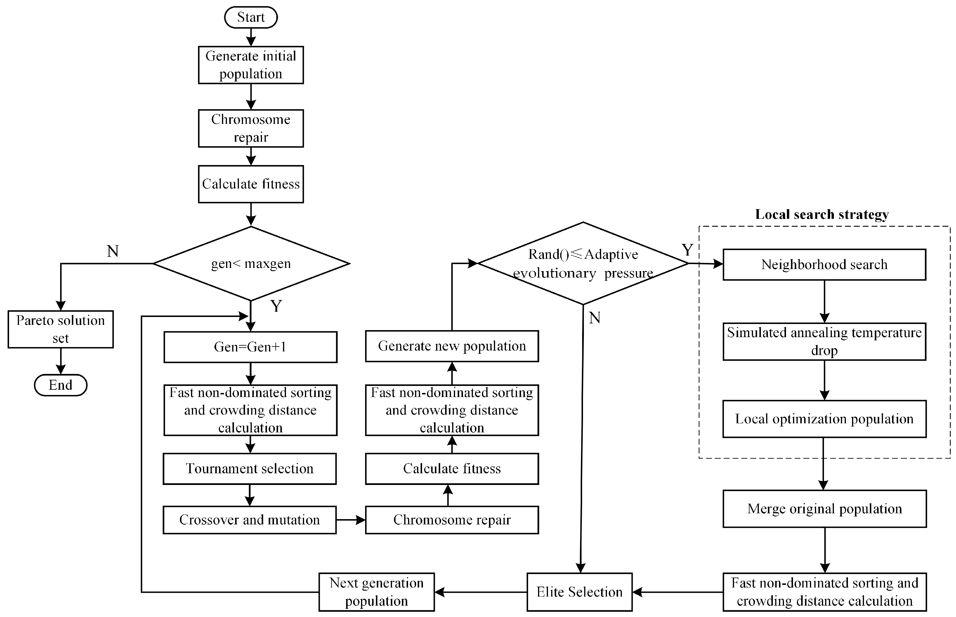
In this section, due to the complexity and numerous constraints of the multi-objective decision model and considering the difficulty of solving the model with commercial solvers and the challenges in obtaining an optimal scheduling solution in a short time, an intelligent optimization algorithm is chosen to solve the model. The NSGA-II algorithm is one of the most commonly used and effective methods for solving multi-objective problems. It has advantages such as fast solving speed and good convergence properties [27,28]. However, the convergence speed of the traditional NSGA-II algorithm is highly sensitive to parameter selection. Moreover, it is prone to falling into local optima during the solving process [29]. To overcome these drawbacks, we propose the ANSGA-NS-SA algorithm. It builds upon the basic framework of the NSGA-II while incorporating three major improvements: dynamic evolutionary parameter control, adaptive selection of evolutionary pressure, and a local optimization strategy based on neighborhood search and simulated annealing. To clearly illustrate the overall computational process of the ANSGA-NS-SA algorithm, Figure 7 visually presents its complete procedure, with key steps detailed in Section 5.1, Section 5.2, Section 5.3, Section 5.4 and Section 5.5. The detailed algorithmic procedure is presented in Algorithm 1. This algorithm aims to achieve rapid convergence of the Pareto solution set while searching for the global optimal solution.
| Algorithm 1: ANSGA-NS-SA |
| . |
| ) do |
| then |
| do |
| do |
| then |
| 27: else |
| 29: end if |
| 31: end while |
| 33: end while |
| 34: end if |
| 41: end while |
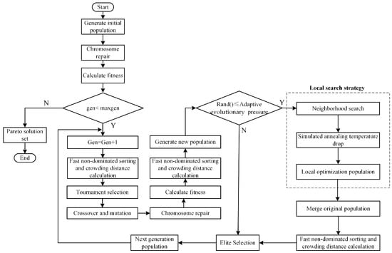
Figure 7.
ANSGA-NS-SA algorithm flowchart.
5.1. Generate Initial Population
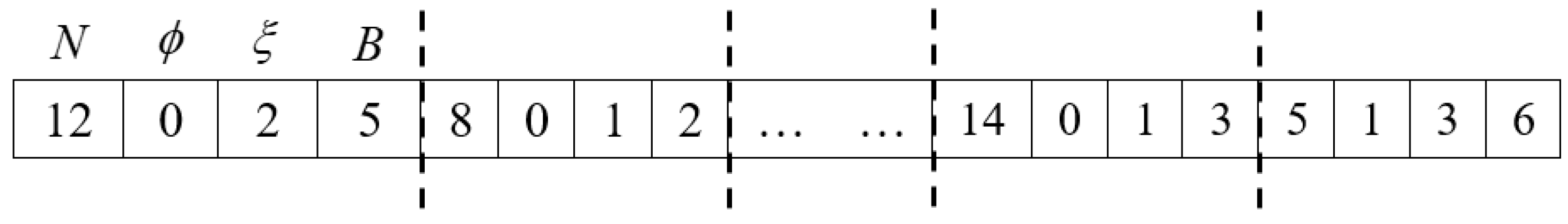
As shown in Figure 8, the gene information of each vessel includes the vessel number , inbound and outbound status , navigation mode , and berth number . The chromosome uses real-value encoding, integrating this vessel information. For example, indicates that vessel 12 departs from berth 5 and uses the main channel in two-way navigation mode. The arrangement of vessel genes on the chromosome represents the sequence of vessels entering and leaving the port. Chromosomes are constructed by randomly permuting vessel genes, followed by generating an initial population of appropriate size (Line 1 in Algorithm 1). During the decoding process, vessel-scheduling information is interpreted based on the chromosome gene sequence, converting it into an optimized vessel entry and departure schedule and the corresponding port traffic management plan.

Figure 8.
Chromosome coding mode.
5.2. Chromosome Repair
There are two situations that can lead to illegal chromosomes in the population. The first situation occurs when an inbound vessel and an outbound vessel are assigned to the same berth, but the inbound vessel’s scheduling time is earlier than the outbound vessel’s departure scheduling time. According to actual port scheduling rules, when inbound and outbound vessels dock at the same berth, the inbound vessel can only be scheduled after the outbound vessel has completed its loading and unloading operations and departed from the berth. The second situation arises when two vessels are sailing in the same direction in one-way navigation mode, and one or more vessels are scheduled in two-way navigation mode between them. In this case, the two-way navigation mode of the vessel must be adjusted to one-way navigation mode. The initialization, mutation, and neighborhood search stages in the algorithm flow may lead to the generation of illegal chromosomes (see lines 2, 12, and 23 in Algorithm 1). Therefore, a repair operator must be designed to automatically adjust the order of inbound and outbound vessels or modify their navigation mode whenever an illegal chromosome is detected, ensuring that the generated solution is feasible.
5.3. Calculating Fitness, Tournament Selection, Crossover, and Mutation
The fitness value is determined by the objective function value. Since both objectives aim to minimize, the objective function values are used as the corresponding fitness values (lines 6, 13, 24, and 36 in Algorithm 1). In the algorithm, the tournament selection method is used to choose the parent individuals (line 9 in Algorithm 1). In each selection, two individuals from the Pareto front are randomly chosen, and the superior chromosome is selected as the parent for the next generation. If the two selected individuals cannot be compared based on dominance, the selection process will be repeated. The crossover operation employs a two-point crossover method. Two distinct chromosomes are randomly selected, and two different crossover points are identified on each chromosome. The vessel numbers between these crossover points are then exchanged (line 10 in Algorithm 1). After the crossover and mutation processes are completed, the remaining genes of the vessels are corrected based on the vessel number information. Considering the significant impact of the selection of crossover and mutation probabilities on the evolutionary speed of the algorithm, the traditional crossover and mutation operators are improved by adopting dynamic crossover operator and mutation operator , as shown in Equations (41) and (42). In these equations, and represent the maximum and minimum crossover probabilities, while and denote the maximum and minimum mutation probabilities. refers to the current iteration number of the algorithm, and represents the maximum number of iterations.
5.4. Adaptive Evolutionary Pressure and Local Search Strategy
To improve the algorithm’s operational efficiency, we introduce the concept of adaptive evolutionary pressure [30], as shown in Equation (43), where the parameter is in the range of [0.1, 0.3]. By comparing a random number within the range of [0, 1] with the adaptive evolutionary pressure, it is determined whether the algorithm should perform local search strategy (line 15 in Algorithm 1). In the early stages of the algorithm’s iterations, the value of the adaptive evolutionary pressure is small, so the algorithm primarily focuses on global search, making it less likely to enter local search. However, in the later stages of the algorithm, as the search space for solutions becomes smaller, the value of increases, making it easier for the algorithm to enter the local search phase in order to find more optimal solutions.
In the algorithm proposed in this paper, a new local optimization strategy is designed (lines 16 to 33 in Algorithm 1). This strategy integrates neighborhood search and simulated annealing algorithms. By selecting a subset of solutions and perturbing their neighborhood structures, it generates higher-quality solutions to prevent the algorithm from getting trapped in local optima during later iterations. The local search strategy begins with the initialization parameters (lines 16 to 18 in Algorithm 1), then the algorithm runs until the stopping criteria are met (line 19 in Algorithm 1). Lines 20 to 33 in Algorithm 1 define a single iteration process. The specific iteration steps are as follows:
Step 1: select the current optimal solution set as the scale for the local search, and set the initial parameters: termination temperature , current temperature , and initialize . Proceed to Step 2.
Step 2: In accordance with the principle that the simulated annealing algorithm can only optimize single-objective problems, randomly select an objective value and use it as the direction for the search optimization. Proceed to Step 3.
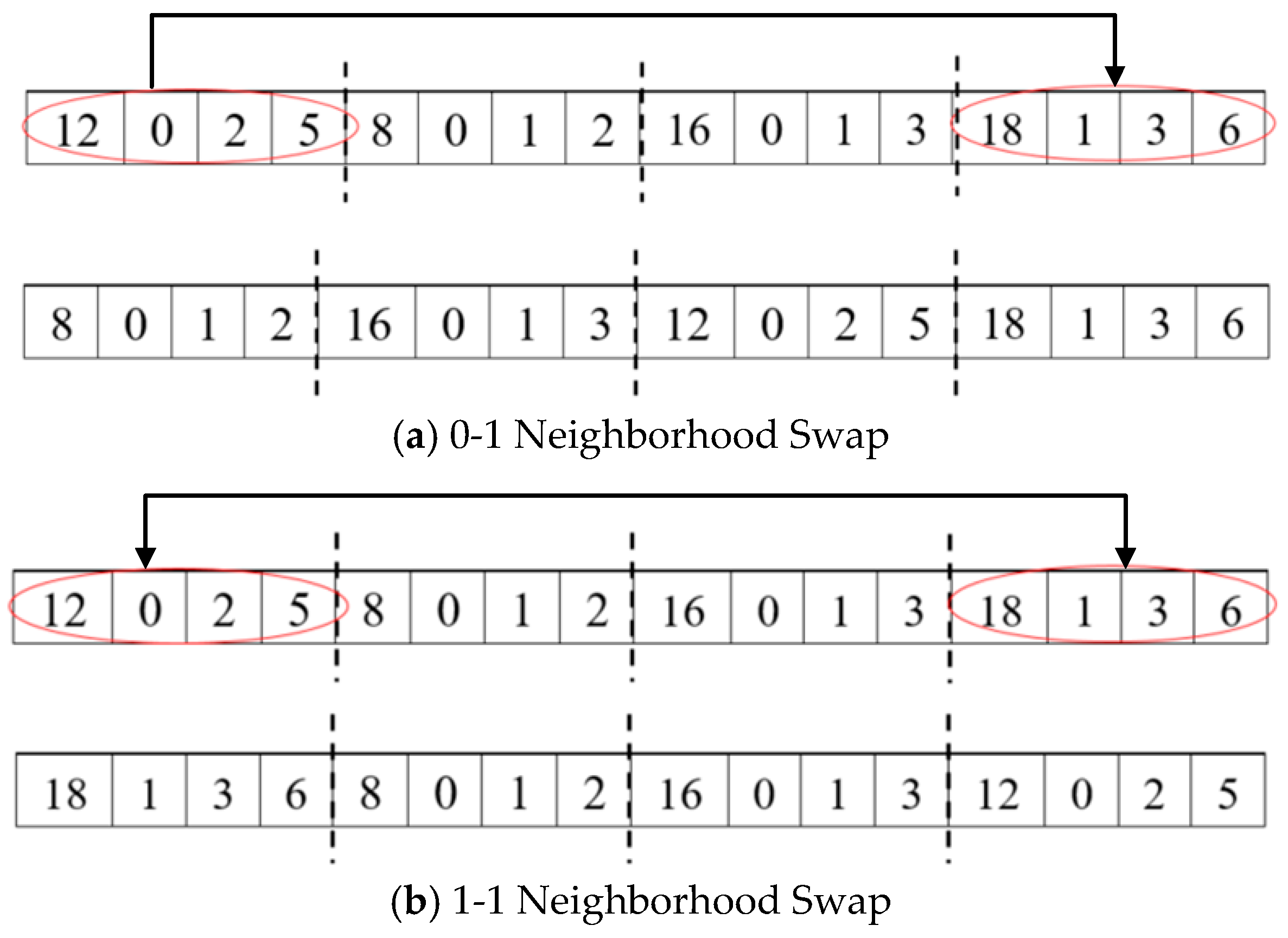
Step 3: Traverse the individuals in the current optimal solution set . For each individual, randomly select a neighborhood swap method to perturb its chromosome, as shown in Figure 9. After completing the neighborhood swap, check the chromosomes. After completing the neighborhood swap, the chromosomes are checked. If any illegal chromosomes are found, the repairing operator is applied to adjust them, ensuring a feasible solution. Proceed to Step 4.
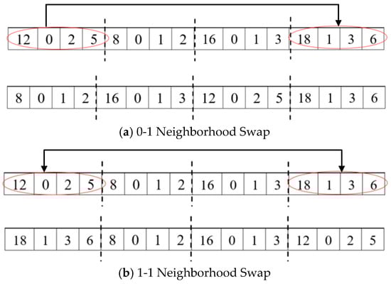
Figure 9.
The 0-1 neighborhood exchange and 1-1 neighborhood exchange.
Step 4: If the perturbed new individual is better than the original individual, add the new individual to the optimized population. Otherwise, based on the probability formula in Equation (44), accept the original individual into the optimized population. In Equation (44), , represents the objective value of the new individual, and represents the average objective value of the population. Proceed to Step 5.
Step 5: Update the current temperature . If , set and proceed to Step 6. Otherwise, proceed to Step 3.
Step 6: If , exit the local search and merge the optimized population with the original population to form the next generation for continued iteration. Otherwise, proceed to Step 2.
5.5. Elite Retention
Elite retention is used to select the new generation of the population. First, the population after the local optimization step is merged with the original population, and the objective function values are recalculated (lines 35 and 36 in Algorithm 1). Then, fast non-dominated sorting and crowding distance comparison are applied to the merged population (lines 37 and 38 in Algorithm 1). Individuals from each non-dominated front are sequentially added to the new population in order of non-domination level, from best to worst. If adding all individuals from a particular non-dominated front causes the new population size to exceed the limit, the individuals are sorted by their crowding distance in descending order, and they are added one by one until the population size limit is met (line 39 in Algorithm 1). This method ensures that high-quality individuals are selected for each generation. Finally, the new population is used as the base population for the next iteration.
6. Numerical Experiments
In this section, numerical experiments are designed based on actual port conditions to evaluate the performance of the proposed vessel-scheduling model and the ANSGA-NS-SA algorithm. Then, comparative experiments with the NSGA-II and FCFS strategies are conducted to demonstrate the advantages of the proposed method in reducing waiting times and improving channel utilization. Finally, sensitivity analysis is performed to verify the robustness and adaptability of our model.
6.1. Case Study
In this subsection, the scheduling of 25 vessels is simulated based on the estuarine port layout described in Section 3, and simulation experiments are conducted according to the model outlined in Section 4. Table 2 presents the navigation rules assigned to vessels in the channel. For vessels requiring tidal navigation, the draft standard is set to 12.5 m. The traffic control time window set by the maritime department is [180.0, 300.0]. Table 3 and Table 4 provide simulated channel segment distance data and specific berth information. The detailed data for the 25 vessels used in the simulation can be found in Table 5.
Table 2.
Rules for the allocation of modes of navigation in channels.
Table 3.
Distance data.
Table 4.
Berth Information.
Table 5.
Vessel information.
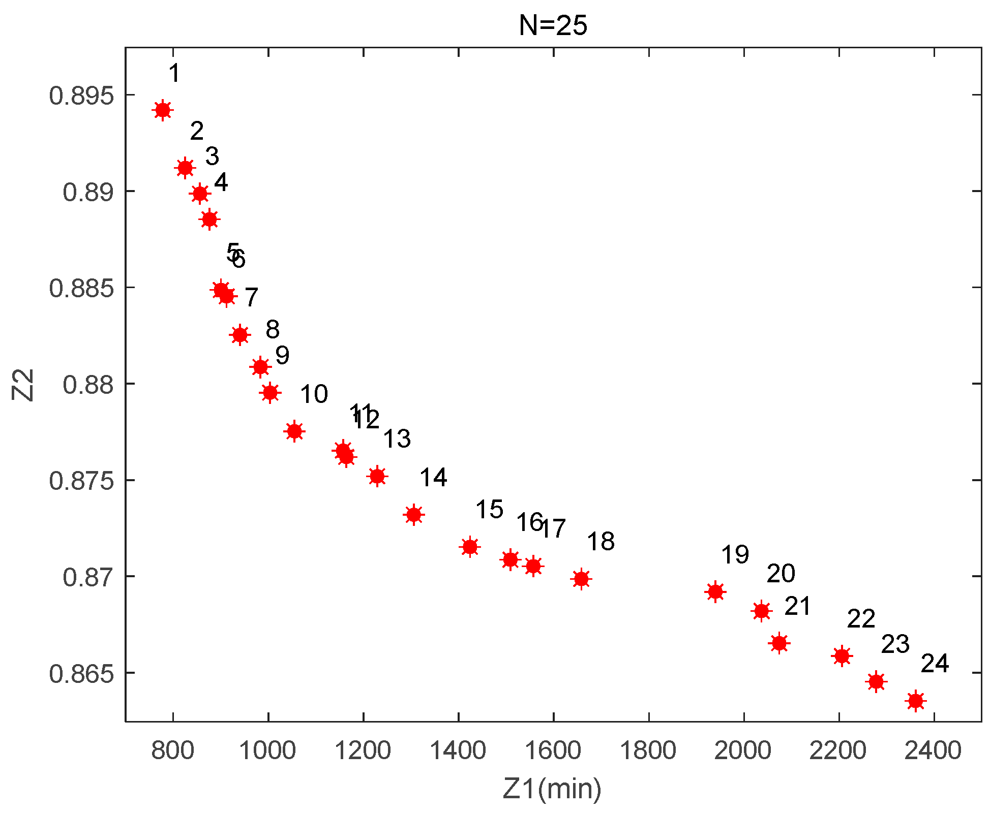
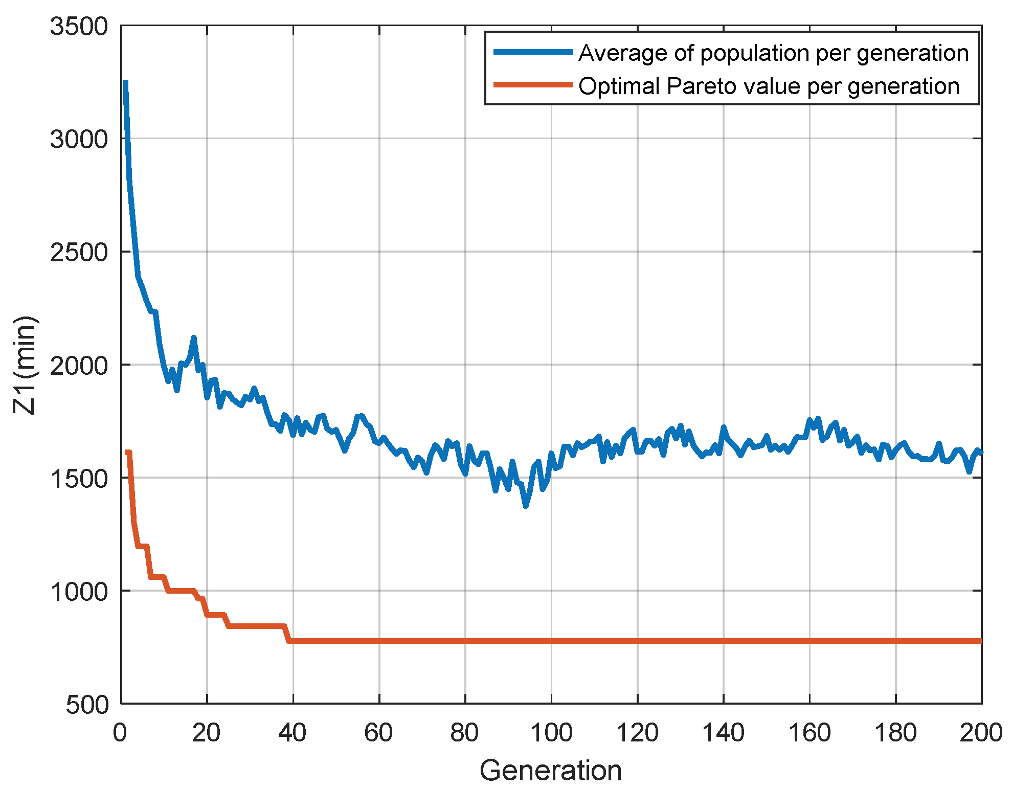
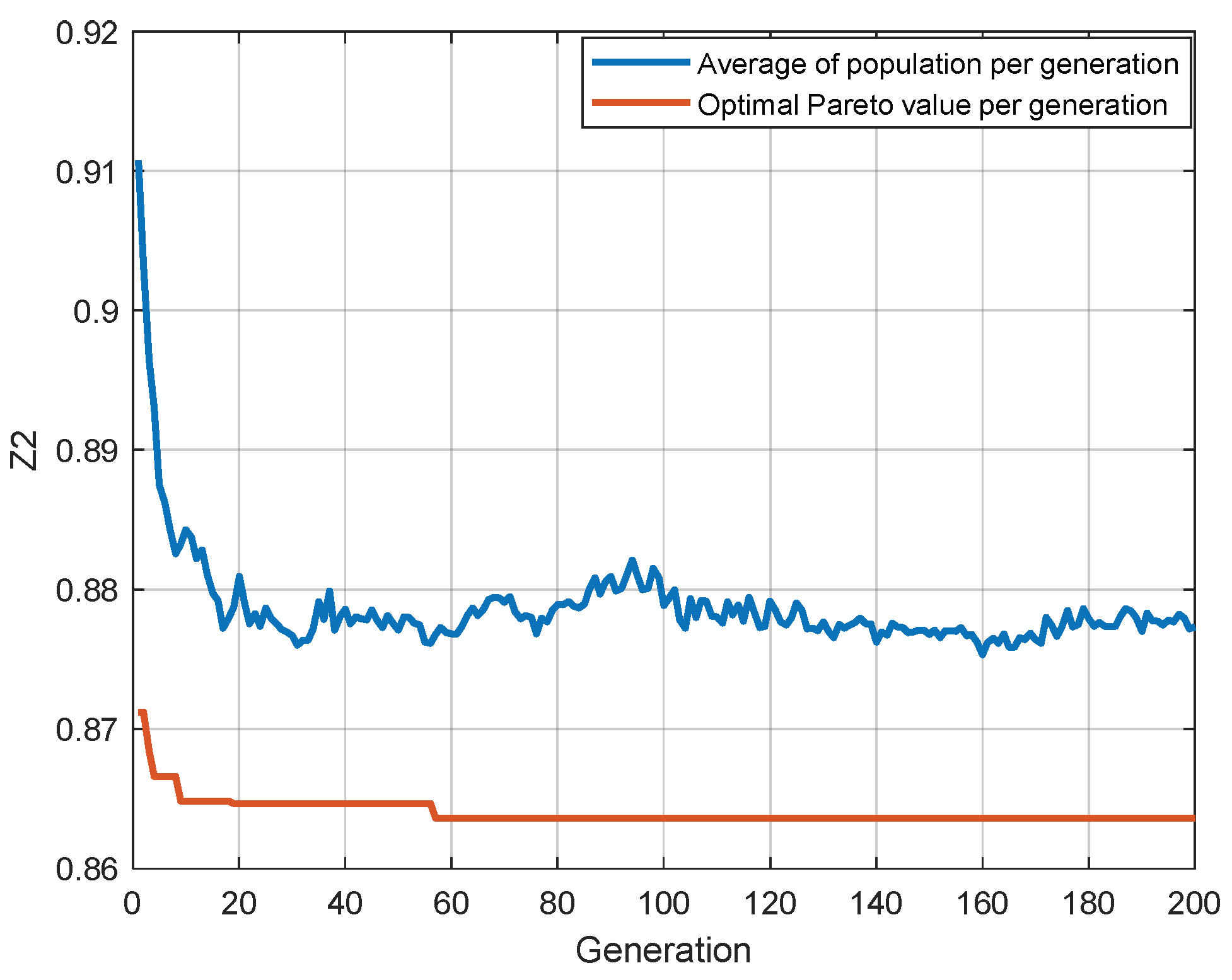
The scheduling process begins at time zero. The initial parameter settings are as follows: population size , maximum number of iterations , maximum crossover rate , minimum crossover rate , maximum mutation rate , minimum mutation rate , and average transit time . The algorithm was executed on a computer with an Intel i7 2.30 GHz processor, 16 GB of RAM, and MATLAB 2020a software. After 200 iterations, the obtained Pareto frontier is shown in Figure 10, with the detailed objective values provided in Table 6. The convergence curves for the optimal values of and , as well as for the population’s average values, are shown in Figure 11 and Figure 12, respectively. converges around the 120th generation, with a minimum total waiting time of 778 min, while converges around the 140th generation, with a minimum channel occupancy ratio of 0.863. As observed in Figure 10 and Table 6, the two objectives of the model are interdependent. When the total vessel waiting time decreases, the total channel occupation ratio increases. This is understandable, as minimizing vessel waiting time requires more flexible scheduling, which may disrupt the overall optimal scheduling sequence. Consequently, more traffic conflicts may arise between vessels, necessitating additional yielding time and ultimately extending the overall scheduling cycle, thereby increasing the total channel occupation ratio. In practical scenarios, the optimal solution typically involves finding a reasonable balance between and , selecting the “optimal Pareto solution” that keeps both objectives at relatively favorable levels, rather than optimizing one objective in isolation.

Figure 10.
Pareto frontier for 25-ship experiments.
Table 6.
Target value of the Pareto front.

Figure 11.
Optimal convergence curves and average convergence curves for each generation of Objective 1.
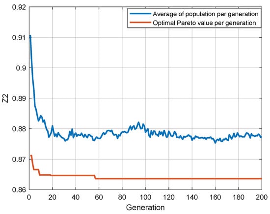
Figure 12.
Optimal convergence curves and average convergence curves for each generation of Objective 2.
6.2. Optimal Solution Selection
In the previous subsection, we derived an optimal Pareto solution set for the 25-vessel case. However, due to conflicting interests between the port authority and shipping companies, it is necessary to evaluate these solutions and select a scheduling plan that maximizes mutual benefits for both parties. To objectively assess the performance of each scheduling plan in the Pareto front, we use the entropy-weighted TOPSIS method. This method calculates the weights of the objectives based on the relative variation in each objective’s information entropy. It is commonly applied to multi-objective decision-making problems [31,32]. The weights of the two objectives, derived using the entropy-weighted method, are shown in Table 7, with the weight for total waiting time being 0.5335 and for total scheduling time being 0.4665. Based on these weights, the TOPSIS evaluation results for the Pareto front solutions are presented in Table 8, which includes the normalized comprehensive scores and the ranking results [33]. The Pareto solution with the highest comprehensive score is solution number 13. Therefore, the scheduling plan corresponding to solution number 13 is selected for model validation.
Table 7.
Target weighting results.
Table 8.
TOPSIS evaluation of the Pareto solution.
6.3. Model Rationality Validation
In this subsection, we validate the rationality of the optimal scheduling solutions selected by the TOPSIS method. Table 9 presents the chromosome decoding results for the Pareto front solution with serial number 13. By extracting the time information encoded within the chromosome, a detailed scheduling plan, including the times at which vessels arrive at various key areas, is obtained, as shown in Table 10.
Table 9.
Chromosomes of Pareto front solution 13.
Table 10.
Time data for vessels at key areas.
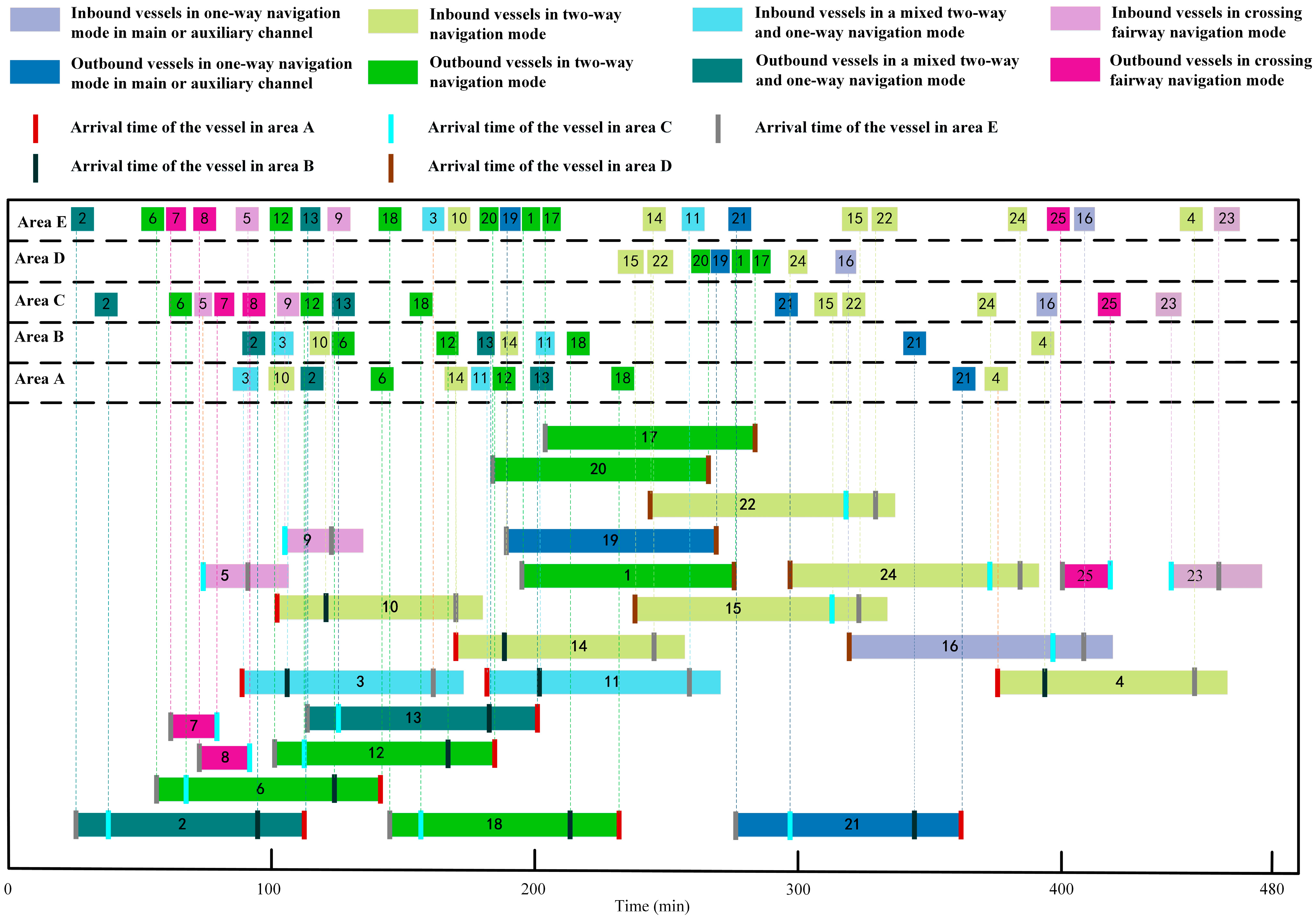
From Table 10, it can be observed that the start scheduling times for all vessels are not earlier than their application times. Vessel 10, vessel 21, and vessel 24 require tidal navigation. Their respective navigation times in the channel are [103.4, 173.6], [281.9, 369.7], and [302.2, 387.1]. These navigation times fall within their corresponding tidal time windows of [90.0, 210.0], [270.0, 390.0], and [270.0, 390.0], respectively, thereby satisfying the tidal time window constraints in the model. It should be noted that outbound vessel 21 exceeds 52 m in width, classifying it as an ultra-wide vessel. According to the regulations in Table 2, ultra-wide vessels must navigate in a one-way direction on all channels, and no other vessels are allowed to navigate in the opposite direction within the same channel segment when an ultra-wide vessel is operating. As shown in the Gantt chart (Figure 13), when outbound vessel 21 enters any channel segment, there are no vessels traveling in the opposite direction within that segment before reaching the next key conflict area, thus meeting the navigation requirements of the channel.

Figure 13.
Gantt chart of optimal vessel-scheduling scheme.
During peak vessel flow periods, to ensure the normal passage of vessels, the maritime authority has set a restricted navigation time window for vessels operating between anchorage no. 2 and the terminal. By observing the scheduling times in Table 10, it can be seen that the vessels (5, 7, 8, 9, 23, 25) that require cross channel operations do not navigate within the restricted time window of [180.0, 300.0], thus meeting the traffic control requirements.
The Gantt chart of the vessel-scheduling plan is shown in Figure 13. By observing the Gantt chart, the sequence of vessels entering and leaving the port and the continuity of each vessel’s navigation can be obtained. Additionally, from the Gantt chart, it can be seen that no traffic conflicts occur when vessels pass through key areas. Combined with the results in Table 10, it is evident that the model assigns appropriate safety time intervals for each vessel when entering and leaving these key areas.
The navigation times of vessels assigned to the same berth are presented in Table 11. From the table, it can be observed that when inbound and outbound vessels are assigned to the same berth, the scheduling time for the outbound vessel precedes that of the inbound vessel. Moreover, when the inbound vessel arrives at area E, the outbound vessel has already left area E and entered the channel, thus fulfilling the berth coordination constraint.
Table 11.
Time data of vessels navigating at the same berth.
6.4. Sensitivity Analysis
In the previous sections, we analyzed the results of the case study involving 25 vessels, confirming the rationality of the proposed model. In this subsection, to validate the superiority of the algorithm designed in this study, we designed cases with different numbers of vessels . For a fair comparison, the model is computed using the ANSGA-NS-SA algorithm, FCFS strategy, and NSGA-II algorithm, and the results are compared. Additionally, considering the rule that no other vessels in the opposite direction are allowed in the channel during the navigation of ultra-wide vessels, this may have a significant impact on the scheduling of other vessels. Therefore, the number of ultra-wide vessels is selected as a parameter for sensitivity analysis to assess its impact on the vessel entry and exit scheduling scheme.
In the validation experiments, each algorithm was run 10 times for each case, and the average values of and were calculated. The results are presented in Table 12. When the number of vessels is 25, and values obtained by the ANSGA-NS-SA algorithm are reduced by 33.8% and 8.8%, respectively, compared to the results of the FCFS strategy, and by 4.1% and 1.5%, respectively, compared to the results of the NSGA-II algorithm. When the number of vessels is 50, and values calculated by the ANSGA-NS-SA algorithm are 1860 min and 0.67, respectively. These are 71.3% and 32.3% lower than the results of FCFS strategy, and 5.4% and 6.9% lower than the results of NSGA-II. Therefore, compared to the FCFS and NSGA-II algorithms, the ANSGA-NS-SA algorithm designed in this paper is more effective in solving the model.
Table 12.
Comparison results in the case of different number of vessels.
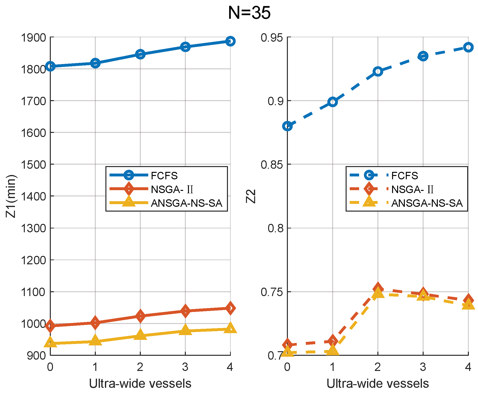
The number of ultra-wide vessels is selected as the sensitivity parameter, and the values of and are calculated using the FCFS strategy, NSGA-II, and ANSGA-NS-SA algorithms, with the results shown in Figure 14. Since the FCFS strategy has already determined the scheduling order of the vessels, it is difficult to arrange a reasonable navigation order for each vessel. When ultra-wide vessels are navigating, vessels traveling in the opposite direction must wait. As the number of ultra-wide vessels increases, and values calculated by the FCFS strategy also continue to rise. In contrast, the NSGA-II and ANSGA-NS-SA algorithms optimize both the scheduling order and navigation patterns of the vessels, resulting in significantly lower and values. As the number of ultra-wide vessels increases, values obtained by the NSGA-II and ANSGA-NS-SA algorithms show a slight increase, but the values do not continuously increase. This indicates that when many ultra-wide vessels are waiting to be scheduled, the scheduling order is adjusted. The vessels are arranged to enter and exit the port in a concentrated manner, thereby reducing the channel occupancy time ratio. Additionally, for cases with the same number of ultra-wide vessels, compared to the FCFS and NSGA-II algorithms, the ANSGA-NS-SA algorithm achieves better solutions. Therefore, the ANSGA-NS-SA algorithm designed in this study demonstrates a clear advantage in terms of stability when solving the model.
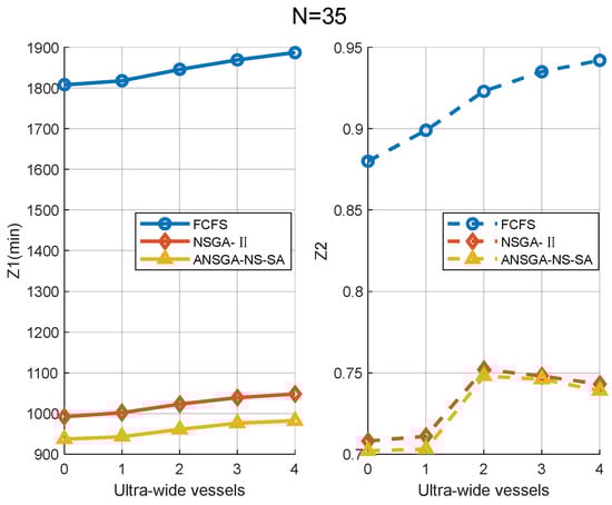
Figure 14.
Number of ultra-wide vessels in relation to the target values.
7. Conclusions
This study investigates the vessel-scheduling problem in an estuarine port with a compound channel, considering the opposing distribution of inner anchorages and terminals. By analyzing the navigation modes and traffic conflicts in a specific estuarine port, we identify five key conflict areas and incorporate constraints such as navigation rules, safety regulations, tidal influences, and traffic control measures. Integrating these factors, we develop a multi-objective scheduling model aimed at minimizing total vessel waiting time and the channel occupancy time ratio. To solve this model, we design the ANSGA-NS-SA algorithm to obtain Pareto front solutions. The entropy-weighted TOPSIS method is then applied to determine the objective weights, identify the optimal solution, and validate the model’s effectiveness. Numerical experiments across different problem sizes demonstrate that, compared to the traditional FCFS strategy and the NSGA-II algorithm, the proposed model and algorithm significantly reduce vessel waiting times and enhance channel utilization. Furthermore, sensitivity analysis confirms the robustness of the model and algorithm under varying vessel traffic conditions.
The proposed model serves as a decision-support tool for port authorities to optimize vessel sequencing, reduce operational costs, and enhance navigational safety. However, real-world scheduling involves additional complexities, such as tugboat service constraints and uncertainties in vessel arrivals and departures. Moreover, incorporating real-time maritime traffic data could further improve the model’s accuracy. Future research should focus on integrating stochastic optimization techniques and real-time scheduling adjustments to enhance adaptability under dynamic maritime conditions.
Author Contributions
Conceptualization, C.L., B.Y., Y.W., X.X., and Y.Z.; methodology, C.L., B.Y., and Y.W.; software, B.Y.; validation, B.Y.; formal analysis, C.L., B.Y., Y.W., Y.Z., and X.X.; investigation, C.L. and B.Y.; resources, C.L. and Y.W.; data curation, C.L.; writing—original draft preparation, C.L. and B.Y.; writing—review and editing, C.L., X.X., and Y.Z.; visualization, C.L. and B.Y.; supervision, C.L.; project administration, C.L. and Y.W.; funding acquisition, C.L. and Y.W. All authors have read and agreed to the published version of the manuscript.
Funding
This research is partially supported by the National Natural Science Foundation of China (72271125) and the Shanghai Sailing Program (21YF1416400).
Data Availability Statement
The original data for this study are presented in the paper, and further inquiries can be directed to the corresponding author.
Conflicts of Interest
The authors declare no conflicts of interest.
Appendix A
Table A1.
Notations.
Table A1.
Notations.
| Symbol | Description |
|---|---|
| Sets | |
| The set of all inbound vessels at anchorage no. 1, no. 2, and no. 3. | |
| The set of all outbound vessels departing towards anchorage no. 1, no. 2 and no. 3. | |
| Parameters | |
| The objective function of the model: the total vessel waiting time and the total channel occupancy time ratio. | |
| to travel from the anchorage to the channel entrance. | |
| The distance between area A and area B, which is the length of the two-way segment. | |
| The distance between area B and area C, or between area B and area E. | |
| The distance between area D and area C, or between area D and area E. | |
| The distance between area D and area E, which is the distance that vessels need to cross the channel. | |
| requires tidal navigation, the value is 1; otherwise, it is 0. | |
| is affected by traffic control, the value is 1; otherwise, it is 0. | |
| The start and end times of the nearest available tidal window for vessels that require tidal navigation. | |
| The start time of the next available tidal window for vessels that require tidal navigation. | |
| The start and end times of the traffic control period. | |
| The start time of the next traffic control period. | |
| at the channel entrance, area B, area C, and area E. | |
| , which refers to the time when inbound vessels leave the anchorage and outbound vessels depart from the berth. | |
| The start scheduling time of the first vessel within the scheduling scheme. | |
| , which refers to the time when inbound vessels arrive at the berth and outbound vessels leave the channel. | |
| The scheduling completion time of the last vessel within the scheduling scheme. | |
| within the channel. | |
| The minimum safety time interval that must be maintained between vessels moving in the same direction and in opposite directions. | |
| Infinite integer | |
| Decision Variables | |
| is outbound. | |
| passes in a mixed one-way and two-way navigation mode. | |
| are moving in the same direction and 0 otherwise. | |
| while moving in the same direction and 0 otherwise. | |
| enters the channel while moving in opposite directions and 0 otherwise. | |
| are in different terminal areas and 0 otherwise. | |
| are assigned the same berth and 0 otherwise. |
References
- UNCTAD. Review of Maritime Transport 2024. Available online: https://unctad.org/publication/review-maritime-transport-2024 (accessed on 10 November 2024).
- Li, L.; Xin, L. Channel arrangement of 12.5 m deepwater channel construction phase I project of Yangtze River downstream Nanjing, Taicang-Nanjing section. Port Waterw. Eng. 2012, 468, 21–25. [Google Scholar]
- Othman, M.K.; Rahman, N.S.F.A.; Ismail, A.; Saharuddin, A. The sustainable port classification framework for enhancing the port coordination system. Asian J. Shipp. Logist. 2019, 35, 13–23. [Google Scholar]
- Xiang, J.; Zhou, C.; Zhao, J.; Latt, M.K.K.; Wen, K.; Gan, L. A micro-network within the port for vessel anchorage selection decision support. Case Stud. Transp. Policy 2024, 18, 101310. [Google Scholar] [CrossRef]
- Zhao, J.; Zhou, C.; Li, Z.; Xu, Y.; Gan, L. Optimization of anchor position allocation considering efficiency and safety demand. Ocean Coast. Manag. 2023, 241, 106644. [Google Scholar] [CrossRef]
- Yang, L.; Liu, J.; Liu, Z.; Luo, W. Grounding risk quantification in channel using the empirical ship domain. Ocean Eng. 2023, 286, 115672. [Google Scholar] [CrossRef]
- Xia, Z.; Guo, Z.; Wang, W.; Jiang, Y. Joint optimization of ship scheduling and speed reduction: A new strategy considering high transport efficiency and low carbon of ships in port. Ocean Eng. 2021, 233, 109224. [Google Scholar] [CrossRef]
- Liang, S.; Yang, X.; Bi, F.; Ye, C. Vessel traffic scheduling method for the controlled waterways in the upper Yangtze River. Ocean Eng. 2019, 172, 96–104. [Google Scholar] [CrossRef]
- Gan, S.; Wang, Y.; Li, K.; Liang, S. Efficient online one-way traffic scheduling for restricted waterways. Ocean Eng. 2021, 237, 109515. [Google Scholar] [CrossRef]
- Zhen, R.; Sun, M.; Fang, Q. Optimization of Inbound and Outbound Vessel Scheduling in One-Way Channel Based on Reinforcement Learning. J. Mar. Sci. Eng. 2025, 13, 237. [Google Scholar] [CrossRef]
- Zhang, B.; Zheng, Z. Model and algorithm for vessel scheduling through a one-way tidal channel. J. Waterw. Port Coast. Ocean Eng. 2020, 146, 04019032. [Google Scholar] [CrossRef]
- Zhang, B.; Zheng, Z.; Wang, D. A model and algorithm for vessel scheduling through a two-way tidal channel. Marit. Policy Manag. 2020, 47, 188–202. [Google Scholar]
- Zhao, K.; Jin, J.G.; Zhang, D.; Ji, S.; Lee, D.-H. A variable neighborhood search heuristic for real-time barge scheduling in a river-to-sea channel with tidal restrictions. Transp. Res. Part E Logist. Transp. Rev. 2023, 179, 103280. [Google Scholar]
- Zheng, H.; Zhu, X.; Li, Z. Optimization algorithm of ship dispatching in container terminals with two-way channel. J. Comput. Appl. 2021, 41, 3049. [Google Scholar]
- Liu, D.; Shi, G.; Kang, Z. Fuzzy scheduling problem of vessels in one-way waterway. J. Mar. Sci. Eng. 2021, 9, 1064. [Google Scholar] [CrossRef]
- Liu, D.; Shi, G.; Hirayama, K. Vessel scheduling optimization model based on variable speed in a seaport with one-way navigation channel. Sensors 2021, 21, 5478. [Google Scholar] [CrossRef]
- Jiang, X.; Zhong, M.; Shi, G.; Li, W.; Sui, Y. Vessel scheduling model with resource restriction considerations for restricted channel in ports. Comput. Ind. Eng. 2023, 177, 109034. [Google Scholar] [CrossRef]
- Jiang, X.; Zhong, M.; Shi, J.; Li, W.; Sui, Y.; Dou, Y. Overall scheduling model for vessels scheduling and berth allocation for ports with restricted channels that considers carbon emissions. J. Mar. Sci. Eng. 2022, 10, 1757. [Google Scholar] [CrossRef]
- Jiang, X.; Zhong, M.; Shi, J.; Li, W. Optimization of integrated scheduling of restricted channels, berths, and yards in bulk cargo ports considering carbon emissions. Expert Syst. Appl. 2024, 255, 124604. [Google Scholar]
- Zhang, X.; Li, R.; Chen, X.; Li, J.; Wang, C. Multi-object-based vessel traffic scheduling optimisation in a compound waterway of a large harbour. J. Navig. 2019, 72, 609–627. [Google Scholar]
- Jia, S.; Wu, L.; Meng, Q. Joint scheduling of vessel traffic and pilots in seaport waters. Transp. Sci. 2020, 54, 1495–1515. [Google Scholar]
- Jia, S.; Li, C.-L.; Xu, Z. Managing navigation channel traffic and anchorage area utilization of a container port. Transp. Sci. 2019, 53, 728–745. [Google Scholar]
- Li, J.; Zhang, X.; Yang, B.; Wang, N. Vessel traffic scheduling optimization for restricted channel in ports. Comput. Ind. Eng. 2021, 152, 107014. [Google Scholar]
- Jia, Q.; Li, R.; Li, J.; Li, Z.; Liu, J. Vessel traffic scheduling optimization for passenger RoRo terminals with restricted harbor basin. Ocean Coast. Manag. 2023, 246, 106904. [Google Scholar]
- Wang, W.; Huang, L.; Ma, J.; Wei, Q.; Guo, Z. Optimizing the number of anchorages based on simulation model of port-channel-anchorage composite system. J. Coast. Res. 2018, 85, 1366–1370. [Google Scholar]
- Liao, Y.; Tu, S.; Wu, Y. Evaluating impacts of anchorages re-provisioning scheme on mega port operations: Simulation approach. Int. J. Ind. Syst. Eng. 2024, 48, 301–320. [Google Scholar]
- Deb, K.; Pratap, A.; Agarwal, S.; Meyarivan, T. A fast and elitist multiobjective genetic algorithm: NSGA-II. IEEE Trans. Evol. Comput. 2002, 6, 182–197. [Google Scholar] [CrossRef]
- Hu, X.; Liang, C.; Chang, D.; Zhang, Y. Container storage space assignment problem in two terminals with the consideration of yard sharing. Adv. Eng. Inform. 2021, 47, 101224. [Google Scholar]
- Zheng, X.; Li, Y.; Liu, H.; Duan, H. A study on a cooperative character modeling based on an improved NSGA II. Multimed. Tools Appl. 2016, 75, 4305–4320. [Google Scholar]
- Houming, F.; Jiaqi, Y.; Mengzhi, M.; Xiaodan, J.; Jili, C.; Zhiwei, Z. Heterogeneous Tramp Ship Scheduling and Speed Optimization with Fuzzy Time Window. J. Shanghai Jiaotong Univ. 2021, 55, 297. [Google Scholar]
- Lai, Y.-J.; Liu, T.-Y.; Hwang, C.-L. Topsis for MODM. Eur. J. Oper. Res. 1994, 76, 486–500. [Google Scholar] [CrossRef]
- Huang, J. Combining entropy weight and TOPSIS method for information system selection. In Proceedings of the 2008 IEEE Conference on Cybernetics and Intelligent Systems, Chengdu, China, 21–24 September 2008; pp. 1281–1284. [Google Scholar]
- Chen, P. Effects of normalization on the entropy-based TOPSIS method. Expert Syst. Appl. 2019, 136, 33–41. [Google Scholar]


Disclaimer/Publisher’s Note: The statements, opinions and data contained in all publications are solely those of the individual author(s) and contributor(s) and not of MDPI and/or the editor(s). MDPI and/or the editor(s) disclaim responsibility for any injury to people or property resulting from any ideas, methods, instructions or products referred to in the content. |
© 2025 by the authors. Licensee MDPI, Basel, Switzerland. This article is an open access article distributed under the terms and conditions of the Creative Commons Attribution (CC BY) license (https://creativecommons.org/licenses/by/4.0/).