Intelligent Detection of Oceanic Front in Offshore China Using EEFD-Net with Remote Sensing Data

Abstract

Oceanic fronts delineate the boundaries between distinct water masses within the ocean, typically marked by shifts in weather patterns and the generation of oceanic circulation. These fronts are identified in research on intelligent oceanic front detection primarily by their significant temperature gradients. The refined identification of oceanic fronts is of great significance to maritime material transportation and ecological environment protection. In view of the weak edge nature of oceanic fronts and the misdetection or missed detection of oceanic fronts by some deep learning methods, this paper proposes an oceanic front detection method based on the U-Net model that integrates Edge-Attention-Module and the Feature Pyramid Network Module (FPN-Module). We conduct detailed statistical analysis and change rate calculation of the oceanic front, and batch process to obtain preliminary high-quality annotation data, which improves efficiency and saves time. Then, we perform manual corrections to correct missed detections or false detections to ensure the accuracy of annotations. Approximately 4800 days of daily average sea temperature fusion data from CMEMS (Copernicus Marine Environment Monitoring Service) are used for analysis, and an Encoder-Edge-FPN-Decoder Network (EEFD-Net) structure is established to enhance the model’s accuracy in detecting the edges of oceanic fronts. Experimental results demonstrate that the improved model’s front identification capability is in strong agreement with fronts segmented and annotated using the threshold method, with IoU and weighted Dice scores reaching 98.81% and 95.56%, respectively. The model can accurately locate the position of oceanic fronts, with superior detection of weak fronts compared to other network models, capturing smaller fronts more precisely and exhibiting stronger connectivity.

1. Introduction

The oceanic front, a narrow transition zone delineating diverse water masses in the ocean, plays a crucial role in marine ecosystems, climate patterns, and ocean dynamics. It is typically characterized by variations in temperature, salinity, and chlorophyll levels, which can be observed as horizontal changes across the ocean surface. Sea Surface Temperature Front (SSTF) is one of the prominent manifestations of oceanic fronts and is widely used for studying their dynamics. The intensity and frequency of oceanic fronts vary seasonally, significantly impacting marine life and weather systems. Accurate detection of oceanic fronts is therefore essential for protecting marine resources, advancing the fisheries sector, optimizing transportation, and understanding ocean-atmosphere interactions [1].

Traditional methods for detecting oceanic fronts [2,3,4,5,6,7,8,9] can be broadly categorized into three types. The first method is the edge detection algorithm, the most common of which is the Canny operator [10], which uses Gaussian filtering to smooth the image and then extracts clear edges by calculating gradients, suppressing noise, and applying double thresholds. However, it is only suitable for detecting objects with fixed edges (such as land, etc.). The second method uses gradient-based algorithms [11], particularly for detecting SSTF, relying on specific gradient thresholds to identify potential front pixels. However, the dependency on high-quality sea surface temperature (SST) data and the neglect of the front’s continuity characteristics limit the effectiveness of these methods. The third method involves statistical modeling, which combines gradient algorithms with histogram analysis to predict potential front areas [12]. While promising, this approach is sensitive to noise and does not adequately model the complex physical processes at play in ocean dynamics.

In recent years, deep learning advancements have greatly influenced fields such as object detection [13,14,15,16] and image segmentation [17,18,19,20,21], leading to new methods for oceanic front detection. The use of artificial intelligence, especially machine learning and neural networks, has played a key role in this progress. Lima et al. [22] were the first to apply convolutional neural networks (CNNs) to oceanic front detection, achieving patch-level detection. Sun [23] and colleagues combined traditional detection methods with CNNs for automated front identification. To address the challenges of limited annotated data and the limitations of traditional algorithms, Li and Hu et al. [24,25] used multi-scale feature fusion and a bidirectional edge detection network, improving detection accuracy. Additionally, Li et al. [26] employed the U-Net architecture to capture crucial information in oceanic front images, successfully detecting and locating key front areas in grayscale sea surface temperature images. Despite these advances, challenges remain, as these methods still show limited accuracy and generalization, particularly in detecting smaller fronts.

Existing research has achieved certain results, but for the physical characteristics of oceanic fronts, traditional methods, and general deep learning techniques struggle to achieve optimal results. To this end, this paper designs a new oceanic front detection model, EEFD-Net, based on the U-Net architecture. By leveraging high-quality labeled datasets and conducting extensive comparative experiments, this research aims to advance the accuracy and robustness of oceanic front detection.

2. Datasets and Data Processing

2.1. Dataset Introduction

The satellite observation data used in this article are derived from the Ocean Sea Temperature and Ice Analysis (OSTIA) product provided by the Copernicus Marine Environment Monitoring Service (CMEMS, https://doi.org/10.48670/moi-00165 (accessed on 1 October 2023). The analysis covers daily average sea surface temperature fusion data from 2009 to 2021, spanning approximately 4800 days. This data product, managed by the Met Office (Exeter, UK) and supplied by IFREMER PU (Plouzané, France), offers a spatial resolution of 0.05° × 0.05° and furnishes information on the regional distribution of sea surface temperature and sea ice. The satellite-derived data includes daily, high-resolution analyses of sea surface temperature across the global ocean and select lakes, formatted in a grid pattern spanning latitudes from −89.97° to 89.97° and longitudes from −179.98° to 179.98°, encompassing the global ocean area. The data format is NetCDF-3 and NetCDF-4. In addition, this data product is not only used for polar environmental monitoring but also serves climate change adaptation, policy and governance, scientific innovation, and many other fields, providing practical value and policy reference significance for research results. In order to verify the feasibility of identifying fronts using this method, 105–135° E and 10–40° N offshore China were selected as the research area.

The downloaded data is loaded in nc file format, and a sea surface temperature image is generated to understand the temperature distribution and provide a basis for subsequent processing, as shown in Figure 1.

2.2. Data Set Annotation

Given the notable temperature variances among adjacent water bodies near oceanic fronts, this paper opts for the temperature gradient as the primary indicator to ascertain the presence of oceanic fronts. Prior to model training, ensuring precise annotation of oceanic front datasets is essential. The threshold method utilizes statistical analysis of extensive data sets to identify the optimal threshold value by analyzing the rate of change in the number of pixels for each gradient measure. This method relies on the data itself and reduces the impact of human subjective judgment. Additionally, the threshold method is simple, avoiding the need for intricate calculations or model training. Further simplification and enhanced efficiency in data processing are achieved through the application of Gaussian filtering and smooth interpolation. To this end, we use the threshold segmentation method to preliminarily mark the oceanic front. Specifically, the threshold segmentation method achieves image division by using designated values as cut-off points categorizing pixels by comparing their gray scale levels to the threshold value. Considering that oceanic front areas usually exhibit higher temperature gradient values, which are more significant than non-frontal areas, we took the following three key steps to define the mean threshold dividing point. First, as shown in Figure 2, we converted the temperature data of the study area into a temperature gradient image, used Gaussian filtering technology to remove subtle noise, and unified the temperature gradient range between 0–0.02 as the image data input to the model. Second, we perform an exhaustive statistical analysis of these gradient values. The uneven distribution of temperature gradient values necessitates caution when directly utilizing them for classification and labeling, as it may lead to inaccurate outcomes. Therefore, we subdivide the temperature gradient value into multiple intervals and perform statistical analysis on the number of pixels in each interval, which helps to accurately identify the gradient change characteristics. Specifically, pixels with gradient values ranging from 0 to 0.001 (inclusive) are categorized under the 0.001 gradient value category. Similarly, pixels with gradient values from 0.001 to 0.002 (inclusive) belong to the 0.002 gradient value category, and so forth. This categorization spans across 21 threshold points, encompassing categories with a gradient value of 0. Finally, after averaging across all training sets, statistical analysis determines the rate of change in pixel counts associated with each gradient value. This detailed analysis accurately identifies the threshold point of the oceanic front.

In oceanography, an oceanic front usually refers to a region where significant spatial gradients in seawater properties (such as temperature) occur. These regions are often associated with higher gradient rates because the very definition of a frontal zone implies the existence of significant differences in physical or chemical properties over short distances. Figure 3 shows in detail the pixel count statistics using all data at different gradient thresholds. Because of the substantial variation in pixel magnitudes, visually representing the trend of the data poses challenges. Therefore, logarithmic transformation is utilized to compress the data range, reduce the impact of outliers, and achieve a more uniform distribution, thus facilitating easier observation and analysis. As can be seen from Figure 3, as the gradient value increases, there is a gradual decrease in the number of pixels. In particular, the rectangular frame in Figure 3 focuses on showing the change in the number of pixels between gradient values 0.013 and 0.017. We know that oceanic front areas usually exhibit higher temperature gradients, which are more obvious than those in the surrounding non-frontal areas. At a higher gradient value of 0.015, there is an obvious turning point in the number of pixels, which may mean that the physical or chemical properties of the area have changed significantly, and it may be possible to separate most of the oceanic front area. Considering that the gradient value of the oceanic front area is much higher than that of the non-oceanic front area, we first assume that the point with a gradient value of 0.015 can be used as a potential threshold point for most frontal areas. Next, further statistical analysis is performed.

When the oceanic front gradient exceeds a certain threshold, the number of pixels with higher gradient values in the frontal area will exceed the number of pixels in the non-frontal area, which means that the rate of change of the number of pixels near the frontal threshold point must be large. In Figure 4, the orange curve is the assumed statistical curve of pixels during non-frontal conditions, while the blue curve reflects the statistical trend of pixels under actual conditions (when there is an oceanic front). Similarly, in order to present the data more intuitively, we used logarithmic transformation and added 1. The rectangular box shows the true statistics of the number of pixels after the potential threshold point. If the gradient change rate near 0.015 is significantly higher than other areas, then this point may mark the boundary or core area of most fronts, because the changes in seawater properties are most obvious at this time. Therefore, we conduct further verification.

To test this theory, we applied the following equation to calculate the rate of change in pixel counts associated with varying gradient values:

$${\displaystyle \frac{∆Num}{∆T}}={\displaystyle \frac{N_1-N_0}{T_1-T_0}}$$

(1)

where, $T_1$ represents a certain gradient threshold, $T_0$ denotes the gradient threshold immediately preceding $T_1$, $N_1$ refers to the number of pixels at the threshold $T_1$, $N_0$ indicates the total number of pixels counted at the gradient threshold $T_0$, and ${\displaystyle \frac{∆Num}{∆T}}$ represents the corresponding rate of change in pixel count.

Figure 5 depicts the results of the rate of change in pixel count across various gradient values. It is worth noting that when the gradient value is 0.015, there is an obvious turning point, and the gradient change rate is relatively obvious; that is, the change in the properties of seawater is the most obvious. This sudden change corresponds to a significant change in the temperature gradient, while the non-oceanic front zone curve is relatively smooth. When finally determining the front zone, it is not necessary to choose the point with the maximum gradient change rate, especially the extreme value at the beginning or end, but to choose a reasonably higher gradient point, such as 0.015, so that the front zone can be captured more stably without being affected by edge effects. Therefore, based on the above analysis, the 0.015 threshold point is used as the critical dividing point of the oceanic front zone for the preliminary annotation data of the oceanic front.

According to the determined threshold points, we preliminarily annotated the oceanic front. Subsequently, the open-source CVAT (Computer Vision Annotation Tool) annotation tool was used to manually correct the preliminary annotation results. The CVAT tool is designed for computer vision tasks. It supports a variety of annotation types, such as rectangular boxes, polygons, points, lines, etc., and is suitable for tasks such as target detection and image segmentation. CVAT provides functions such as team collaboration, task management, data import, and export and supports integration with machine learning frameworks. It can provide an efficient annotation interface and flexible correction functions, making the manual correction process more convenient and accurate. In Figure 6, (a) is the temperature gradient image of the study area on 1 January 2022, (b) is the image of the study area annotated by the threshold segmentation method on 1 January 2022, and (c) is the annotated image of the study area after manual correction on 1 January 2022. In the final annotated image (c), the red area clearly identifies the location of the oceanic front. Through this step, we successfully completed the annotation of the oceanic front and provided a reliable annotation dataset for subsequent model training and application.

We successfully completed the annotation of the oceanic front by combining the threshold segmentation method with manual correction. The initial threshold segmentation method identified the main oceanic front features, while the manual correction further supplemented the details, such as the Beibu Gulf front, the eastern coastal front of Hainan Island, and the Kuroshio front, and optimized the identification of the frontal boundary. For the tidal mixing front (TMF) along the offshore edge of the Jiangsu Shoal/Bank (Subei Shoal/Bank), which was not clearly identified by mathematical methods due to gradient and other reasons, a manual correction was performed to further improve the annotation. The final annotation results clearly identified the location of the oceanic front, providing a high-quality dataset for subsequent model training and application.

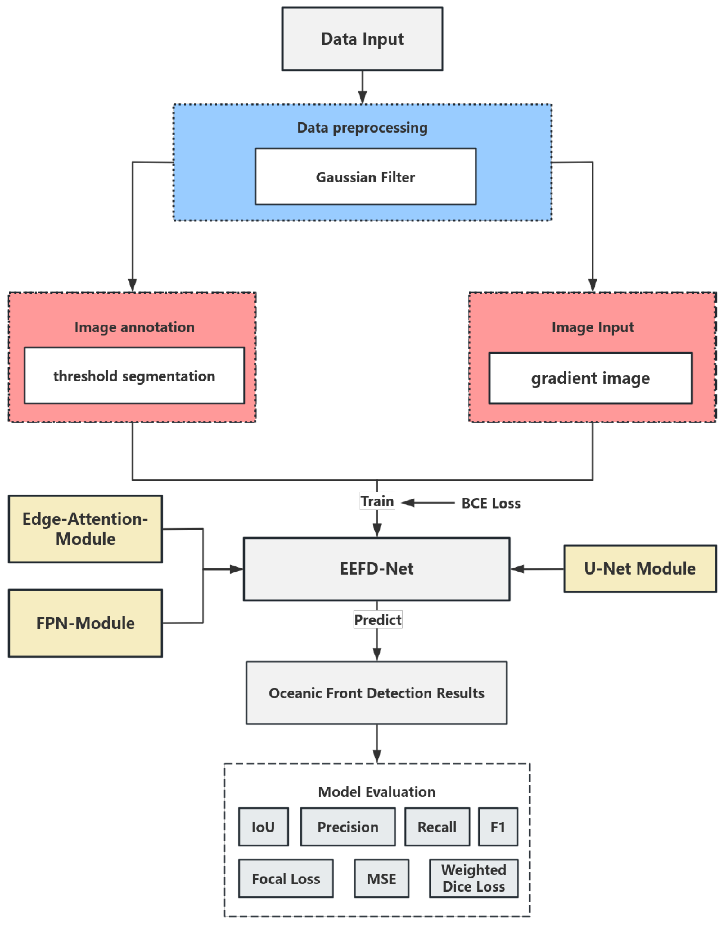
3. Model Description

3.1. Existing Algorithm

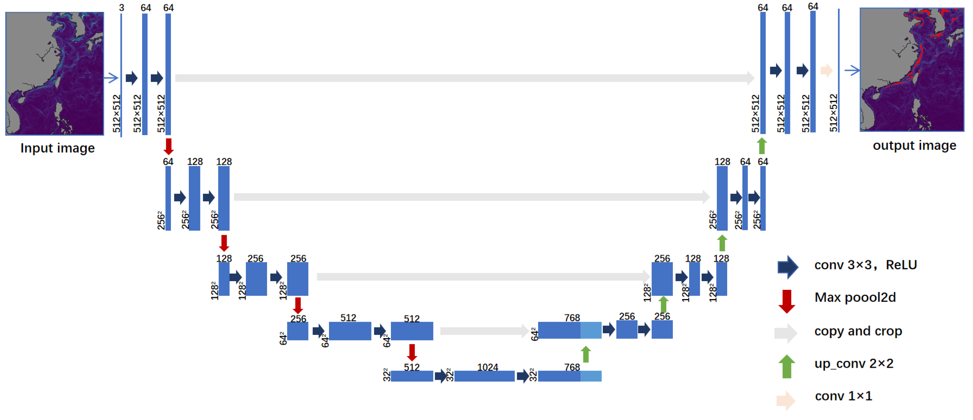
3.1.1. Basic Principles of U-Net

U-Net, as a popular convolutional neural network (CNN) architecture, was originally designed for medical image segmentation tasks by Olaf Ronneberger, Philipp Fischer, and Thomas Brox [27]. The core idea is to effectively capture the contextual information in the image and accurately locate the area of interest by constructing a symmetrical encoder-decoder structure. The network structure includes two key components: the encoder, which performs downsampling by extracting high-level features and reducing spatial resolution, and the decoder, which is responsible for upsampling to restore spatial details and generate the final output. As the encoder reduces the size of the input image, it creates feature maps; these maps are then used by the decoder to produce segmentation results. As shown in Figure 7, in the U-Net network architecture for identifying s, the input data is a 512 × 512 × 3 RGB three-channel oceanic front temperature gradient image and then traverses the encoder’s feature extraction module, which employs a sequence of 3 × 3 convolution and 2 × 2 max pooling operations to extract features from the input image. At each processing stage, the feature maps gain more channels, capturing complex semantic details. The encoder downsamples them to enhance feature abstraction by reducing spatial resolution. Each downsampling module includes max pooling and dual convolution operations, enabling the network to learn features from coarse to fine. Within its decoder segment, the U-Net utilizes a series of upsampling modules to incrementally restore the feature map to the original size of the input image. In each upsampling module, the feature map is upsampled and combined with the encoder’s corresponding layer, followed by a double convolution to retain more oceanic front details during segmentation. Finally, the U-Net model outputs a 512 × 512 × 1 segmentation image where each pixel is categorized as either oceanic front or non-oceanic front, thereby effectively segmenting oceanic fronts.

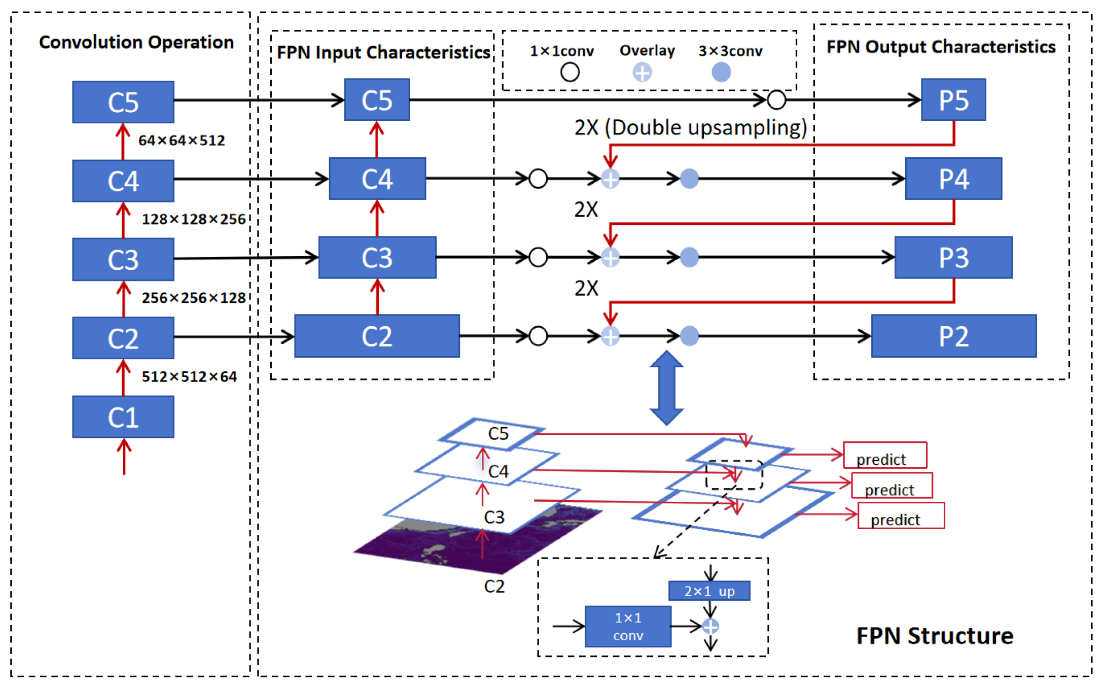
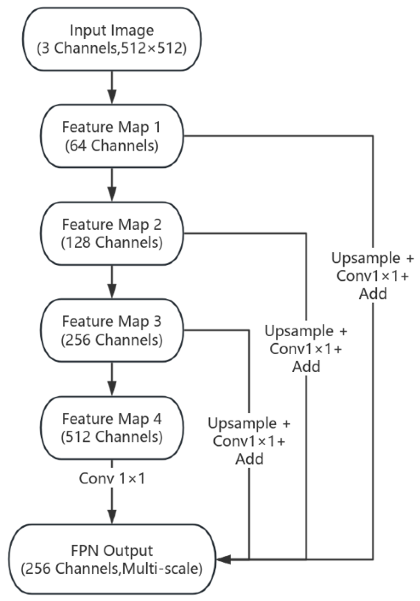
3.1.2. Basic Principles of FPN

The Feature Pyramid Network (FPN) [28] is an innovative network architecture, as shown in Figure 8. It extracts multi-scale feature maps through successive convolution operations (C1-C5). FPN progressively upsamples higher-level feature maps using a double upsampling operation and fuses them with lower-level feature maps, generating output feature maps (P2-P5) of varying resolutions. These multi-scale feature maps enable the network to better handle objects of different sizes in object detection tasks, facilitating accurate bounding box and class predictions. The core idea behind FPN is to construct a feature pyramid that fuses feature information at different scales through top-down and bottom-up connections [29]. This structure allows the model to effectively interpret objects across multiple scales, significantly enhancing the accuracy and robustness of detection and segmentation tasks. In the context of oceanic front detection, deep network features provide rich semantic information but lack sufficient representation of small spatial details, while shallow features capture rich spatial information but are limited in semantic depth. By combining the strengths of both deep and shallow features, FPN enhances oceanic front detection algorithms, improving their ability to capture both semantic and spatial information. The primary objective of FPN is to address the challenges of detecting and segmenting objects at varying scales, thereby boosting the overall performance and robustness of the model.

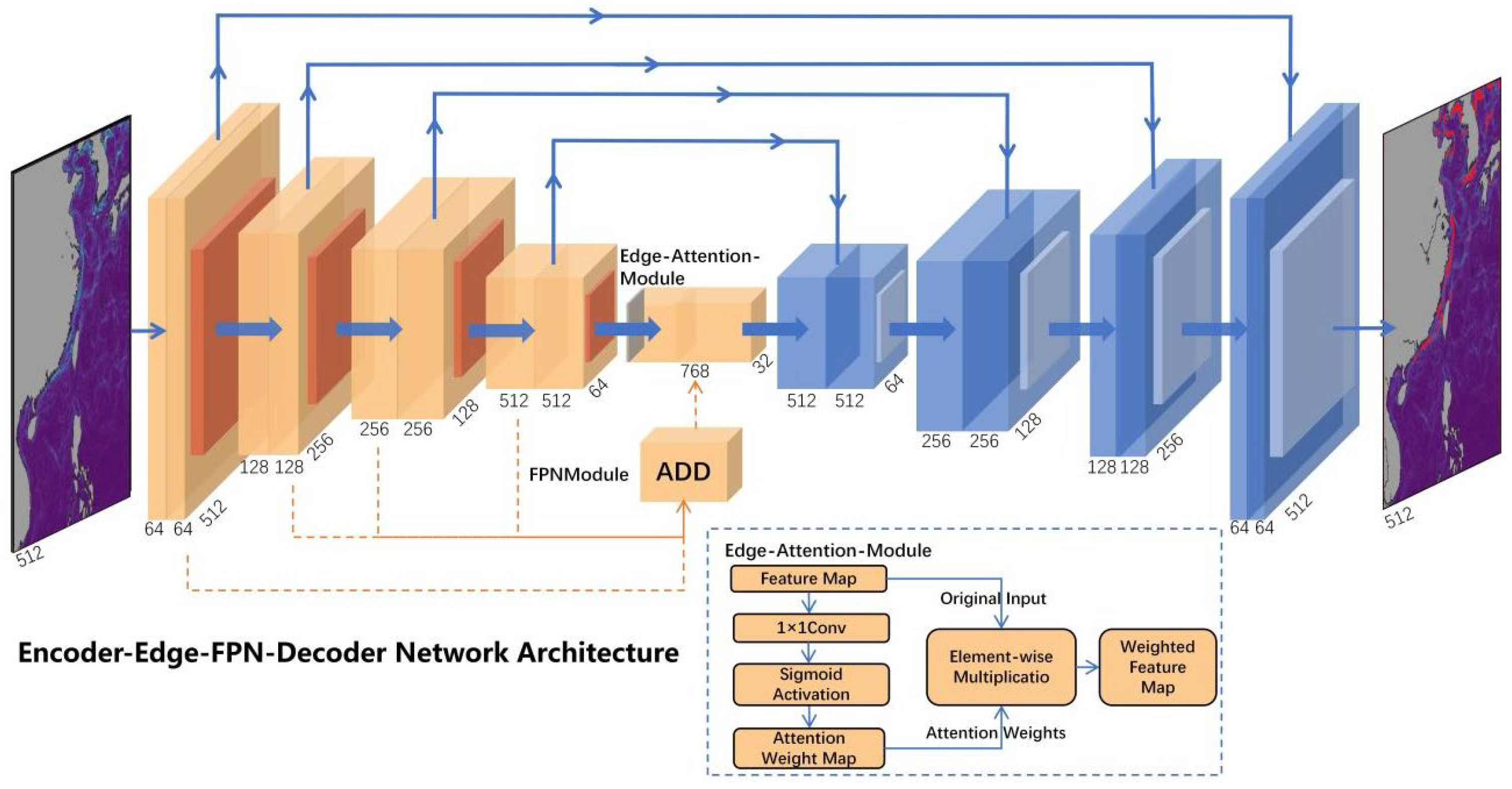
3.2. Improve Algorithm (EEFD-Net)

The U-Net architecture ingeniously employs skip connections to link feature maps between the encoder and decoder, preserving the detailed information of oceanic front edges efficiently. However, this architecture is limited by its lack of a multi-scale feature fusion mechanism when dealing with oceanic fronts with significant scale changes, which, to a certain extent, affects the ability to identify oceanic front targets. FPN can achieve the extraction and fusion of features at different scales by building a multi-level feature pyramid, which significantly improves the model’s ability to identify targets at different scales. However, when dealing with problems such as oceanic fronts with small target characteristics and weak edge characteristics, the information transmission of FPN may still be insufficient, leading to the loss of spatial information. In order to overcome these limitations, this paper integrates Edge-Attention-Module and FPN-Module based on the U-Net network architecture to build a new network called Encoder-Edge-FPN-Decoder (EEFD-Net), aiming to enable intelligent identification of oceanic fronts.

The overall architecture of EEFD-Net is illustrated in Figure 9. The U-Net encoder, serving as the model’s entry point, is tasked with extracting initial features from the oceanic front image input, which is of size 512 × 512 × 3. The encoding structure comprises two convolutional layers, employing a 3 × 3 convolutional kernel to keep the dimensions of the output feature map consistent, following each layer with batch normalization and a ReLU activation function. Through consecutive convolution and downsampling operations, the feature map undergoes spatial size reduction while enhancing feature depth and capturing increasingly abstract features. A spatial attention mechanism (Edge-Attention-Module) is added after the encoder to calculate edge attention weights, which indirectly enhances the quality of feature representation by focusing on local edges of the image, highlights edge features, and enhances the model’s ability to perceive edges. The Edge-Attention-Module structure is depicted within the rectangular box in Figure 9. A two-dimensional convolution layer with a 1 × 1 convolution kernel is used to transform the input feature map into a single-channel edge attention map, and the attention weight is compressed to between 0 and 1 through the sigmoid activation function for subsequent element-wise multiplication operations. After the Edge-Attention-Module (i.e., the transition part of the encoder-decoder), an FPN-Module is incorporated, as illustrated in Figure 10. The FPN-Module takes feature maps with input levels of 64, 128, 256, and 512 channels and unifies them into 256 channels through 1 × 1 convolutions, followed by upsampling and addition. That is, starting from the deepest layer of the feature map, features are successively upsampled to match the size of the feature map from the previous layer and then integrated element-wise with the feature map of the preceding (higher resolution) layer. This process iterates from the deepest to the shallowest feature map, with each step involving the addition of the upsampled output of the current layer to the feature map of the previous layer. This achieves feature upsampling and fusion. Ultimately, multiple levels of feature maps (×1, ×2, ×3, ×4) are generated, where each level’s feature map is a downsampled version of the previous one. After multi-scale feature extraction, the U-Net network is reconstructed, comprising four upsampling modules. These modules gradually restore the spatial dimensions of the feature maps and merge features from both the downsampling path and the FPN. Each module includes an upsampling operation followed by a double convolution operation. Finally, a 1 × 1 convolution layer converts the final feature map to an output with the same number of classes as the target (with the number of oceanic front classes being 1). The output feature map has a size of 512 × 512 × 1.

EEFD-Net effectively integrates the feature extraction and reconstruction capabilities of U-Net. It preserves the advantages of U-Net in maintaining edge details while enhancing the model’s capacity to recognize objects at varying scales through the introduction of a multi-scale feature fusion mechanism. Furthermore, the integration of the Edge-Attention-Module enables the model to emphasize the edge characteristics of the oceanic front, thereby improving its ability to detect and delineate boundaries with greater precision.

4. Experimental Environment and Results

4.1. Experimental Preparation

The construction and training of this model were completed under the PyTorch deep learning framework (version 1.13.0, https://pytorch.org, accessed on 1 October 2023). A new oceanic front automatic detection model was built based on U-Net integrating Edge-Attention-Module and FPN-Module. When labeling the training set, the pixels in the image are divided into oceanic front types and non-oceanic front types according to the set threshold. In this context, pixel points equal to or exceeding the threshold are categorized as oceanic front types, while those below the threshold are classified as non-oceanic front types.

The effectiveness of deep learning in oceanic front detection is highly dependent on sufficient training samples. Therefore, this article selects 13 years of daily average sea temperature fusion data from 2009 to 2021 and divides it according to a ratio of 8:2. Among them, 80% of the data is used for model training, aiming to capture and learn the complex relationships and patterns between oceanic front features, and the remaining 20% of the data is used for model verification to comprehensively evaluate the performance and generalization ability of the model during the training process. To address potential outlier issues in oceanic front data, gaussian filtering technology was employed during the data preprocessing phase to smooth the image and minimize noise interference. Subsequently, a threshold segmentation method was used to construct an oceanic front label data set based on the threshold value. After preparing the data and labels, we input them into the model for training. In oceanic front training, it’s typically treated as a binary classification problem; thus, the binary cross-entropy function serves as the loss function. It is suitable for situations where the output is a probability distribution or a logical value (0 or 1) and can help the model maximize the similarity between the predicted results and the real labels. This loss function has a smaller penalty for correct classification predictions, but a larger penalty for incorrect classification predictions, which can encourage the model to better learn to distinguish between oceanic front areas and non-frontal areas. The binary cross-entropy loss function can be represented by the following formula:

$$L\left(y,\widehat{y}\right)=-[y\times \log \left(\widehat{y}\right)+\left(1-y\right)\times \log \left(1-\widehat{y})\right]$$

(2)

where y is the true value (0 or 1) and $\widehat{y}$ is the predicted value (a probability value between 0 and 1). Specifically, for each pixel, the binary cross-entropy loss function calculates the difference between the prediction and the true label, and these differences are accumulated and averaged to obtain the loss value for the entire oceanic front image. Throughout the training, the Adaptive Moment Estimation (Adam) optimization algorithm [30] is employed to minimize the loss value, thereby enhancing the model’s accuracy in identifying oceanic fronts.

Finally, the model will undergo testing and evaluation using the 2022 test set to validate its real application effectiveness. The specific process of identifying oceanic fronts is shown in Figure 11.

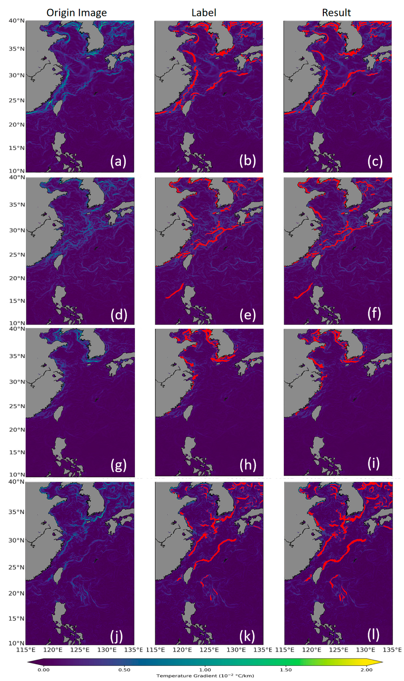
4.2. Result and Analysis

Through systematic experimentation, validation, and parameter optimization, the optimal settings for oceanic front detection were established. The network achieves satisfactory performance with a learning rate of 0.0001, a batch size of 16, and 100 training epochs. Notably, the network begins to detect oceanic fronts after approximately 100 iterations. To ensure stability and generalization, the identification algorithms were evaluated following training. For improved visual clarity, certain land regions were omitted. A fundamental component of the model training process was the implementation of a two-step methodology for generating high-quality labeled data. Initially, mathematical and statistical techniques were utilized to determine an optimal sea surface temperature (SST) gradient threshold, which served as the basis for an automated batch annotation of oceanic fronts. However, given the inherent limitations of purely algorithmic labeling—such as the potential for false positives and missed detections—a subsequent manual refinement phase was introduced. This human-in-the-loop approach enabled the correction of annotation inaccuracies, thereby enhancing the precision and consistency of the dataset. The finalized dataset, integrating both data-driven statistical analysis and expert validation, was subsequently employed for model training, leading to improved recognition of oceanic front structures with greater accuracy and robustness. Figure 12 illustrates the seasonal variability of oceanic fronts in 2022, providing a clearer comparison of their spatiotemporal patterns.

Among them, (a–c) corresponds to the oceanic front image on 15 January 2022, (d–f) corresponds to the oceanic front image on 15 April 2022, (g–i) corresponds to the oceanic front image on 15 July 2022, (j–l) corresponds to the oceanic front image on 15 October 2022. The images not only demonstrate the performance of the network in different seasons but also highlight its accuracy under different oceanic front distributions. In Figure 12, the original temperature gradient image, the labeled temperature gradient image, and the test result image are also included, represented by letters (a) to (l), respectively, where (a,d,g,j) are the original images of the oceanic front, (b,e,h,k) are oceanic front images annotated after manual correction., (c,f,i,l) are oceanic front images identified using EEFD-Net.

The image results show that regardless of whether it is a season with frequent or fewer oceanic fronts, the oceanic fronts identified by EEFD-Net are highly consistent in shape with those annotated using manual correction. As observed in Figure 12, the oceanic fronts refined through manual correction exhibit greater completeness and continuity during subsequent testing. The identified frontal structures demonstrate improved coherence, effectively capturing continuous frontal features. Notably, previously indistinct or undetected fronts—such as the Kuroshio Front and the Bohai Coastal Front—were more accurately recognized compared to the initial annotations based solely on mathematical methods. For instance, the temperature-salinity front in the central South China Sea during spring and the Zhejiang-Fujian Coastal Front in autumn were successfully delineated with higher precision. Furthermore, oceanic fronts across different seasons, whether continuous or discontinuous, were largely identifiable, providing a solid foundation for the further refinement of deep neural networks in ultra-fine oceanic front detection. These findings indicate that the proposed model is capable of accurately capturing subtle frontal features, highlighting its high precision and robustness in oceanic front identification.

4.3. Model Validation

After model training, objectively assessing its performance and effectiveness enables better utilization of the model in practical decision-making scenarios. For the binary classification task of oceanic fronts, data can be categorized into four groups based on their conditions and prediction outcomes: true positives (TP), false positives (FP), true negatives (TN), and false negatives (FN), with the total number of true and false instances equating to the total sample count. TP indicates the number of pixels correctly identified as oceanic fronts, TN indicates the number of pixels correctly identified as non-oceanic fronts, FN represents the number of pixels falsely identified as non-oceanic fronts, and FP represents the number of pixels falsely identified as oceanic fronts. The classification results are summarized in

Table 1. Confusion matrix.

	Predicted Result
	Positive	Negative
Actual Condition
True	TP (True Positive)	TN (True Negative)
False	FP (True Negative)	FN (False Negative)

, known as the confusion matrix.

To more accurately demonstrate the effectiveness of EEFD-Net in identifying oceanic fronts, a comparative evaluation of different models is conducted based on the confusion matrix of the binary classification results. The Intersection over Union (IoU), also referred to as the Jaccard index, is a metric utilized to quantify the intersection between two bounding boxes (or regions) [31]. IoU values range from 0 to 1, with higher values signifying increased overlap between predicted and actual outcomes. The formula for calculating IoU is as follows:

$$IoU={\displaystyle \frac{Area of Overlap}{Area of Union}}$$

(3)

Since there is a very serious imbalance in the oceanic front image data set, the weighted Dice coefficient is more suitable for scenarios with unbalanced sample sizes. It’s a better criterion for assessing model quality than classification accuracy. The Dice coefficient [32] measures the similarity between two sets and is commonly employed in image segmentation tasks to gauge sample similarity. Here is the formula:

$$D(P,T)={\displaystyle \frac{2|P\cap T|}{|P\cup T|}}$$

(4)

Here, P is the predicted area of the oceanic front, and T is the area where the oceanic front actually exists. $|P\cap T|$ indicates the size of the intersection between the prediction result and the real label, that is, the number of oceanic front pixels shared by the two sets. $|P\cup T|$ represents the sum of pixels in the predicted area and the real area.

The weighted Dice coefficient is a variant of the Dice coefficient that better handles class imbalance by weighting the number of true and false positives. Its value also varies between 0 and 1, where higher values signify greater alignment between the predicted and true results. The weighted Dice coefficient calculation formula is as follows:

$$D_{weighted}=\alpha D_{front}+\beta D_{bg}$$

(5)

Here, $D_{front}$ is the Dice coefficient of the oceanic front area, and $D_{bg}$ is the Dice coefficient of the non-oceanic front area. $\alpha$ and $\beta$ are expressed as the weighted coefficients of the oceanic front and non-oceanic front areas, respectively. Since the study area is large and the non-frontal areas are large, the value of $\beta$ should be relatively small. After many experiments and statistical analysis, the values of $\alpha$ and $\beta$ were 0.98 and 0.02, respectively.

The precision rate indicates the ratio of correctly predicted positive category samples to all samples predicted as positive by the model. It assesses how accurately the model identifies positive samples. Recall rate represents the ratio of correctly predicted positive samples to all true positive samples. It gauges the model’s ability to identify true positives. The F1 score, calculated as the harmonic mean of precision and recall, offers a comprehensive evaluation of the model’s performance. It ranges from 0 to 1, with higher scores denoting superior model performance. The formulas for precision, recall, and F1 score are as follows:

$$Precision={\displaystyle \frac{TP}{TP+FP}}$$

(6)

$$Recall={\displaystyle \frac{TP}{TP+FN}}$$

(7)

$$F1=2\times {\displaystyle \frac{Precision\times Recall}{Precision+Recall}}$$

(8)

Mean Squared Error (MSE) is a frequently utilized loss function in regression analysis. It calculates the average of the squared differences between the predicted values and the actual values. The formula for MSE loss is as follows:

$$MSE Loss={\displaystyle \frac{1}{N}}\sum _{i=1}^N{(y_i-\widehat{y_i})}^2$$

(9)

where y is the true value and $y_i$ is the predicted value.

Focal loss is a loss function utilized to address the challenge of unevenness categories. It is mainly used to solve the problem of foreground and background category imbalance in target detection tasks. Focal loss will reduce the weight of easily classified samples, making the model pay more attention to those samples that are difficult to classify, thereby improving the model’s learning ability for difficult samples. In the problem of oceanic front detection, the traditional cross-entropy loss function makes it easy to classify them as non-front samples under the condition of category imbalance, causing the model to tend to learn more features of non-front samples. Focal loss modifies the weighting of simple samples through the incorporation of an attenuation factor, consequently diminishing the influence of straightforward samples and prompting the model to prioritize challenging ones. The following presents the formula for Focal loss:

$$FL\left(P_t\right)=-{\left(1-P_t\right)}^{\gamma }·\log \left(P_t\right)$$

(10)

where, $P_t$ denotes the predicted probability value, and $\gamma$ serves as a positive adjustment parameter utilized to modify the sample weight. It usually takes a smaller value. This article takes the value 0.1.

Weighted Dice loss [33] is the loss function of the weighted Dice coefficient. $L_{Dice}$ is the loss function value of the model. Its calculation formula is as follows:

$$L_{Dice}=1-D_{weighted }$$

(11)

To comprehensively validate the enhanced performance of the improved model in detecting oceanic fronts following the integration of two additional modules, we carried out a series of comparative experimental evaluations. We compared the model in this article with traditional oceanic front detection methods and some modules in the model in detail. These models include the traditional gradient method, the FPN model, a hybrid model that combines FPN and Edge-Attention-Module, and U-Net model, the combined model of U-Net network and Edge-Attention-Module, and the hybrid model of U-Net and FPN, and verify the effectiveness of the introduced modules. The comprehensive findings of the comparison are outlined in

Table 2. Evaluation indicators for different model test sets.

Module	Metrics (%)
	IoU	Weighted Dice	Precision	Recall	F1 Score
FPN	95.79	93.21	95.72	96.15	95.93
FPN + Edge-Attention	97.80	94.21	95.56	95.32	95.44
U-Net	96.04	95.36	95.68	96.05	95.86
U-Net + Edge-Attention	97.77	95.18	94.21	96.00	95.10
U-Net + FPN	95.23	93.54	95.86	95.55	95.70
EEFD-Net	98.81	95.56	96.32	96.13	96.22

.

As shown in Table 2, the EEFD-Net model, by integrating U-Net, FPN-Module, and Edge-Attention-Module, significantly outperforms traditional methods across multiple evaluation metrics. The optimal value for each evaluation metric is emphasized in bold, clearly indicating that the model achieves superior performance in terms of IoU, weighted Dice, precision, recall, and F1 score. The model achieves an IoU of 98.81%, which far exceeds that of other comparative models, fully demonstrating the high overlap rate between the predicted and actual regions. This is imperative for accurately identifying and pinpointing the location of oceanic fronts. Furthermore, the model achieves a weighted Dice coefficient of 95.56%, reflecting its robustness to class imbalance. Additionally, the EEFD-Net model’s precision reaches 96.32%, and its recall is 96.13%. These high values indicate the model’s exceptional ability to minimize both false positives (low false positive rate) and false negatives (low false negative rate), indicating robust performance. The F1 Score reaches 96.22%, the highest among all models, effectively proving the model’s advantage in maintaining a balance between detection precision and recall.

In order to verify the effect of the loss function of the EEFD-Net model in this article, MSE loss, Focal loss, and Dice loss were put into different models for comparison. The results are listed in

Table 3. Different model test set loss functions.

Module	Loss Function (%)
	MSE Loss (10−2)	Focal Loss (10−2)	Dice Loss (10−2)
FPN	0.729	9.126	6.790
FPN + Edge-Attention	0.555	8.549	5.790
U-Net	0.151	2.974	4.640
U-Net + Edge-Attention	0.760	2.189	4.827
U-Net + FPN	0.453	3.329	6.460
EEFD-Net	0.034	1.650	4.440

.

As evident in Table 3, an analysis of the loss functions across various models on the test set underscores the lowest values in bold. It can be seen that the EEFD-Net model exhibits significant superiority, particularly by showing the lowest loss values across various loss function metrics. This model significantly optimizes the accuracy and robustness of oceanic front detection.

The exceptional performance of EEFD-Net is primarily attributed to its innovative network architecture and integrated module design. The U-Net architecture provides the model with strong feature extraction capabilities, while the FPN-Module optimizes the integration of multi-scale features, enabling the model to fully capture oceanic front information at different scales. The introduction of the Edge-Attention-Module further enhances the model’s focus on edges and details, thereby improving the accuracy of oceanic front detection.

5. Discussion

At present, compared with previous oceanic front detection methods, the EEFD-Net proposed in this paper has certain advantages in both method and performance and is more targeted at the refined detection of oceanic fronts. From the test results, it can be seen that the model performs well in the identification of oceanic fronts in winter and spring, especially in the detection of the Kuroshio front and the East China Sea nearshore front, and can accurately identify the position and morphology of the front, which is highly consistent with the annotation results. Although the oceanic fronts are relatively weak in summer and autumn, the model can still effectively identify the main fronts, especially in the sea area between 30 degrees and 35 degrees north latitude. Overall, the model performs well in the identification of strong oceanic fronts, can accurately capture the spatial distribution and spatiotemporal changes of the fronts, and shows high accuracy and stability.

To further validate the efficacy of the proposed method for oceanic front identification, a comparison is made with the traditional threshold method, as well as with current state-of-the-art image segmentation algorithms and neural network learning models [8,25,26,34,35,36]. All experiments are conducted under identical experimental conditions using the same dataset, with the validation set employed for model prediction and performance evaluation. The results are summarized in

Table 4. Metric results for different models.

Module	Metrics (%)
	mIoU	mWDSC
Threshold Method	76.77	69.29
Deeplab v3+	89.93	87.25
GoogleNet Inception	95.90	93.96
SQNet	91.63	92.84
LSENet	85.58	93.56
BPFANet	93.99	95.40
EEFD-Net	98.81	95.56

, where the mean Intersection over Union (mIoU) and the mean Weighted Dice Similarity Coefficient (mWDSC) are reported as metrics of model performance.

The experimental results in Table 4 demonstrate that EEFD-Net outperforms all other models, achieving a mIoU of 98.81% and a mWDSC of 95.56% (The best indicators are in bold), which are significantly higher than the other methods. This clearly illustrates the superior performance of EEFD-Net in oceanic front detection. Notably, EEFD-Net excels in identifying weak and small-scale oceanic fronts, accurately capturing faint edges, and effectively integrating multi-scale information.

Despite its strong performance, EEFD-Net has limitations, including sensitivity to noisy data and extreme sea conditions. The model’s performance is also influenced by the diversity and quality of the training data. Moreover, the current approach primarily utilizes sea surface temperature data, and the potential integration of other oceanographic variables, such as salinity and chlorophyll concentration, remains unexplored. Future work could focus on incorporating multi-source remote sensing data and exploring semi-supervised or self-supervised learning methods to improve the model’s adaptability.

In conclusion, this study presents EEFD-Net as an effective and advanced tool for oceanic front detection, offering significant improvements over existing methods. Its ability to detect weak edges and integrate multi-scale information makes it highly useful for ocean observation and decision-making in marine-related fields.

6. Conclusions

The detection of the oceanic front is crucial for marine environmental management, playing significant roles in climate, weather, biodiversity, and fisheries. Monitoring the oceanic front helps optimize resource management and reduce the risk of environmental disasters. A profound comprehension of their dynamics facilitates the protection and utilization of these vital regions, thereby safeguarding the health and fostering sustainable development of marine ecosystems.

Addressing the weak edge characteristics and data imbalance of the oceanic front and leveraging advancements in deep learning for image segmentation and object detection, this paper improves the network structure based on the U-Net model by integrating the Edge-Attention-Module and FPN-Module, establishing an accurate and efficient oceanic front detection model named EEFD-Net. The EEFD-Net model not only excels in accurately locating oceanic front, achieving IoU and weighted Dice scores of 98.81% and 95.56%, respectively, but also surpasses other network models in detecting weak fronts, particularly in capturing fine frontal features with higher precision and efficiency. Additionally, through comparative testing of different loss functions, EEFD-Net demonstrates its superiority in reducing prediction errors and optimizing performance. These achievements showcase the potential of combining deep learning techniques with specialized modules to enhance the automatic recognition capability of the oceanic front and provide an invaluable analytical instrument for marine science research, it streamlines the exploration of material transport and ecological conservation in aquatic environments.

Future endeavors will entail delving deeper into the adaptability and robustness of the model by utilizing broader environmental datasets and intricate scenarios, thereby enhancing our comprehension of the underlying mechanisms that shape the oceanic front and analyzing seasonal variation characteristics to achieve more comprehensive and accurate oceanic front identification.

References

1. Bost, C.; Cotté, C.; Bailleul, F.; Cherel, Y.; Charrassin, J.B.; Guinet, C.; Ainley, D.G.; Weimerskirch, H. The importance of oceanographic fronts to marine birds and mammals of the southern oceans. J. Mar. Syst. 2008, 78, 363–376. [Google Scholar] [CrossRef]
2. Canny, J. A computational approach to edge detection. IEEE Trans. Pattern Anal. Mach. Intell. 1986, PAMI-8, 679–698. [Google Scholar] [CrossRef]
3. Cayula, J.F.; Cornillon, P. Edge detection algorithm for SST images. J. Atmos. Oceanic Technol. 1992, 9, 67–80. [Google Scholar] [CrossRef]
4. Belkin, I.M.; O’Reilly, J.E. An algorithm for oceanic front detection in chlorophyll and SST satellite imagery. J. Mar. Syst. 2009, 78, 319–326. [Google Scholar] [CrossRef]
5. Liu, Y.; Chen, W.; Chen, Y.; Chen, W.; Ma, L.; Meng, Z. Ocean front reconstruction method based on K-means algorithm iterative hierarchical clustering sound speed profile. J. Mar. Sci. Eng. 2021, 9, 1233. [Google Scholar] [CrossRef]
6. Simhadri, K.K.; Iyengar, S.S.; Holyer, R.J.; Lybanon, M.; Zachary, J. Wavelet-based feature extraction from oceanographic images. IEEE Trans. Geosci. Remote Sens. 1998, 36, 767–778. [Google Scholar] [CrossRef]
7. Kostianoy, A.G.; Ginzburg, A.I.; Frankignoulle, M.; Delille, B. Fronts in the Southern Indian Ocean as inferred from satellite sea surface temperature data. J. Mar. Syst. 2004, 45, 55–73. [Google Scholar] [CrossRef]
8. Hopkins, J.; Challenor, P.; Shaw, A.G.P. A new statistical modeling approach to ocean front detection from SST satellite images. J. Atmos. Ocean. Technol. 2010, 27, 173–191. [Google Scholar] [CrossRef]
9. Pi, Q.L.; Hu, J.Y. Analysis of sea surface temperature fronts in the Taiwan Strait and its adjacent area using an advanced edge detection method. Sci. China Earth Sci. 2010, 53, 1008–1016. [Google Scholar] [CrossRef]
10. Sangeetha, D.; Deepa, P. FPGA implementation of cost-effective robust Canny edge detection algorithm. J. Real-Time Image Process. 2019, 16, 957–970. [Google Scholar] [CrossRef]
11. Oram, J.J.; McWilliams, J.C.; Stolzenbach, K.D. Gradient-based edge detection and feature classification of sea-surface images of the Southern California Bight. Remote Sens. Environ. 2008, 112, 2397–2415. [Google Scholar] [CrossRef]
12. Kirches, G.; Paperin, M.; Klein, H.; Brockmann, C.; Stelzer, K. GRADHIST—A method for detection and analysis of oceanic fronts from remote sensing data. Remote Sens. Environ. 2016, 181, 264–280. [Google Scholar] [CrossRef]
13. Dong, D.; Shi, Q.; Hao, P.; Huang, H.; Yang, J.; Guo, B.; Gao, Q. Intelligent Detection of Marine Offshore Aquaculture with High-Resolution Optical Remote Sensing Images. J. Mar. Sci. Eng. 2024, 12, 1012. [Google Scholar] [CrossRef]
14. Cheng, C.; Hou, X.; Wang, C.; Wen, X.; Liu, W.; Zhang, F. A Pruning and Distillation Based Compression Method for Sonar Image Detection Models. J. Mar. Sci. Eng. 2024, 12, 1033. [Google Scholar] [CrossRef]
15. Zhao, Z.-Q.; Zheng, P.; Xu, S.-T.; Wu, X. Object detection with deep learning: A review. IEEE Trans. Neural Netw. Learn. Syst. 2019, 30, 3212–3232. [Google Scholar] [CrossRef]
16. Li, Z.; Zheng, B.; Chao, D.; Zhu, W.; Li, H.; Duan, J.; Zhang, X.; Zhang, Z.; Fu, W.; Zhang, Y. Underwater-Yolo: Underwater Object Detection Network with Dilated Deformable Convolutions and Dual-Branch Occlusion Attention Mechanism. J. Mar. Sci. Eng. 2024, 12, 2291. [Google Scholar] [CrossRef]
17. Yanowitz, S.D.; Bruckstein, A.M. A new method for image segmentation. Comput. Vis. Graph. Image Process. 1989, 46, 82–95. [Google Scholar] [CrossRef]
18. Cheng, H.D.; Jiang, X.H.; Sun, Y.; Wang, J. Color image segmentation: Advances and prospects. Pattern Recognit. 2001, 34, 2259–2281. [Google Scholar] [CrossRef]
19. Plaksyvyi, A.; Skublewska-Paszkowska, M.; Powroźnik, P. A Comparative Analysis of Image Segmentation Using Classical and Deep Learning Approach. Adv. Sci. Technol. Res. J. 2023, 17, 127–139. [Google Scholar] [CrossRef]
20. Udupa, J.K.; LeBlanc, V.R.; Zhuge, Y.; Imielinska, C.; Schmidt, H.; Currie, L.M.; Hirsch, B.E.; Woodburn, J. A framework for evaluating image segmentation algorithms. Comput. Med. Imaging Graph. 2006, 30, 75–87. [Google Scholar] [CrossRef]
21. Minaee, S.; Boykov, Y.; Porikli, F.; Plaza, A.J.; Kehtarnavaz, N.; Terzopoulos, D. Image segmentation using deep learning: A survey. IEEE Trans. Pattern Anal. Mach. Intell. 2021, 44, 3523–3542. [Google Scholar] [CrossRef]
22. Lima, E.; Sun, X.; Dong, J.; Wang, H.; Yang, Y.; Liu, L. Learning and transferring convolutional neural network knowledge to ocean front recognition. IEEE Geosci. Remote Sens. Lett. 2017, 14, 354–358. [Google Scholar] [CrossRef]
23. Sun, X.; Wang, C.; Dong, J.; Lima, E.; Yang, Y. A multiscale deep framework for ocean fronts detection and fine-grained location. IEEE Geosci. Remote Sens. Lett. 2018, 16, 178–182. [Google Scholar] [CrossRef]
24. Li, Q.; Zhong, G.; Xie, C.; Hedjam, R. Weak edge identification network for ocean front detection. IEEE Geosci. Remote Sens. Lett. 2021, 19, 1501905. [Google Scholar] [CrossRef]
25. Hu, J.; Li, Q.; Xie, C.; Zhong, G. Ocean front detection with bi-directional progressive fusion attention network. IEEE Geosci. Remote Sens. Lett. 2023, 20, 1502005. [Google Scholar] [CrossRef]
26. Li, Y.; Liang, J.; Da, H.; Chang, L.; Li, H. A deep learning method for ocean front extraction in remote sensing imagery. IEEE Geosci. Remote Sens. Lett. 2021, 19, 1502305. [Google Scholar] [CrossRef]
27. Ronneberger, O.; Fischer, P.; Brox, T. U-Net: Convolutional networks for biomedical image segmentation. In Proceedings of the Medical Image Computing and Computer-Assisted Intervention—MICCAI 2015, Munich, Germany, 5–9 October 2015; Lecture Notes in Computer Science; Navab, N., Hornegger, J., Wells, W., Frangi, A., Eds.; Springer: Cham, Switzerland, 2015; Volume 9351, pp. 234–241. [Google Scholar] [CrossRef]
28. Lin, T.Y.; Dollár, P.; Girshick, R.; He, K.; Hariharan, B.; Belongie, S. Feature pyramid networks for object detection. In Proceedings of the IEEE Conference on Computer Vision and Pattern Recognition, Honolulu, HI, USA, 21–26 July 2017; pp. 2117–2125. [Google Scholar] [CrossRef]
29. Zhu, L.; Lee, F.; Cai, J.; Yu, H.; Chen, Q. An improved feature pyramid network for object detection. Neurocomputing 2022, 483, 127–139. [Google Scholar] [CrossRef]
30. Bock, S.; Weiß, M. A proof of local convergence for the Adam optimizer. In Proceedings of the 2019 International Joint Conference on Neural Networks (IJCNN), Budapest, Hungary, 14–19 July 2019; IEEE: New York, NY, USA, 2019; pp. 1–8. [Google Scholar] [CrossRef]
31. Zhou, D.; Fang, J.; Song, X.; Guan, C.; Yin, J.; Dai, Y.; Yang, R. IoU loss for 2D/3D object detection. In Proceedings of the 2019 International Conference on 3D Vision (3DV), Quebec City, QC, Canada, 16–19 September 2019; IEEE: New York, NY, USA, 2019; pp. 85–94. [Google Scholar] [CrossRef]
32. Guindon, B.; Zhang, Y. Application of the dice coefficient to accuracy assessment of object-based image classification. Can. J. Remote Sens. 2017, 43, 48–61. [Google Scholar] [CrossRef]
33. Liu, Y.C.; Tan, D.S.; Chen, J.C.; Cheng, W.-H.; Hua, K.-L. Segmenting hepatic lesions using residual attention U-Net with an adaptive weighted dice loss. In Proceedings of the 2019 IEEE International Conference on Image Processing (ICIP), Taipei, Taiwan, 22–25 September 2019; IEEE: New York, NY, USA, 2019; pp. 3322–3326. [Google Scholar] [CrossRef]
34. Felt, V.; Kacker, S.; Kusters, J.; Pendergrast, J.; Cahoy, K. Fast ocean front detection using deep learning edge detection models. IEEE Trans. Geosci. Remote Sens. 2023, 61, 4204812. [Google Scholar] [CrossRef]
35. Yang, Y.; Lam, K.M.; Sun, X.; Dong, J.; Lguensat, R. An efficient algorithm for ocean-front evolution trend recognition. Remote Sens. 2022, 14, 259. [Google Scholar] [CrossRef]
36. Niu, R.; Tan, Y.; Ye, F.; Gong, F.; Huang, H.; Zhu, Q.; Hao, Z. SQNet: Simple and fast model for ocean front identification. Remote Sens. 2023, 15, 2339. [Google Scholar] [CrossRef]
Figure 1. Sea surface temperature map for 1 January 2022.
Jmse 13 00618 g001
Figure 2. Temperature gradient image on 1 January 2022, with thresholds uniformly between 0 and 0.02.
Jmse 13 00618 g002
Figure 3. Number of pixels corresponding to different gradient thresholds (log of Frequency + 1). The box represents the enlarged view of the number of pixels (statistical frequency) between 0.013 and 0.017 gradient thresholds.
Jmse 13 00618 g003
Figure 4. The number of pixels (log of Frequency + 1) of oceanic fronts and non-oceanic fronts (hypothetical) under different gradient thresholds. Assume that the gradient value 0.015 is the threshold point. The rectangular box represents the statistical number of pixels after the threshold point.
Jmse 13 00618 g004
Figure 5. The gradient change rate of pixel counts under varying gradient thresholds is illustrated. The red curve represents the smoothed connected gradient rate curve achieved through cubic spline interpolation.
Jmse 13 00618 g005
Figure 6. Before and after comparison of annotated images. (a) is the temperature gradient image of the study area on 1 January 2022, (b) is the image of the study area annotated by the threshold segmentation method on 1 January 2022, and (c) is the annotated image of the study area after manual correction on 1 January 2022.
Jmse 13 00618 g006
Figure 7. U-Net architecture.
Jmse 13 00618 g007
Figure 8. Feature Pyramid Network architecture.
Jmse 13 00618 g008
Figure 9. EEFD-Net overall architecture.
Jmse 13 00618 g009
Figure 10. FPN-Module backbone architecture.
Jmse 13 00618 g010
Figure 11. Oceanic front identification process based on EEFD-Net.
Jmse 13 00618 g011
Figure 12. Test result comparison image. (ac) represent the image on 15 January 2022, (df) represent the image on 15 April 2022, (gi) represent the image on 15 July 2022, (jl) represent the image on 15 October 2022. (a,d,g,j) are the original temperature gradient images, (b,e,h,k) are the labeled temperature gradient images, and (c,f,i,l) are the test result images.
Jmse 13 00618 g012