Abstract
Particle Image Velocimetry (PIV) is essential in experimental fluid mechanics, providing nonintrusive flow field measurements. Among the recent advances in PIV algorithms, deep-learning-based optical flow estimation is distinguished by its high spatial and temporal resolution, as well as remarkable efficiency, especially RAFT-PIV, which is based on Recurrent All-Pairs Field Transforms (RAFT). However, RAFT-PIV is extremely susceptible to experimental conditions characterized by low signal-to-noise ratios (SNR), leading to unacceptable errors. This study proposes PIV-RAFT-EN, an enhanced RAFT-based algorithm integrating image denoising, enhancement, and optical flow estimation via a Multi-Task Convolutional Neural Network (MTCNN). Evaluations on synthetic and real-world low-SNR data demonstrate its superior accuracy and efficiency. PIV-RAFT-EN offers a reliable solution for precise PIV measurements in challenging environments, including practical applications like vehicle water entry.
1. Introduction
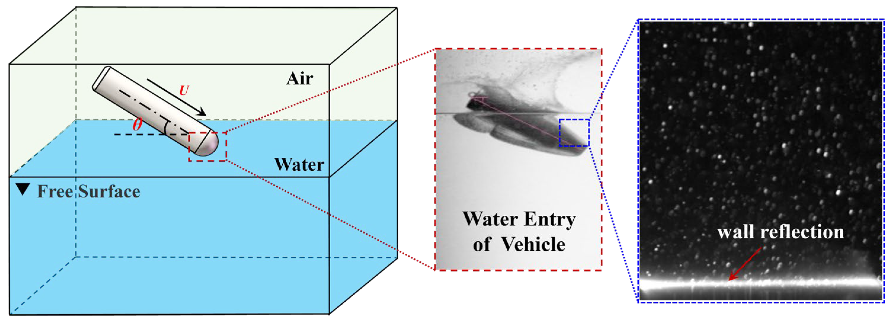
Flow measurement techniques are widely used in both engineering applications and scientific research [1,2,3,4,5,6,7,8,9,10,11]. Complex flow occurs in the thin boundary layer, and the flow field near the wall of the underwater vehicle directly affects its core technical indicators (such as drag, cavitation, attitude stability, etc.). However, it is extremely difficult to directly measure the near-wall flow field and vortex structure, especially the flow field near the wall. The most prevalent flow field velocimetry technique is Particle Image Velocimetry (PIV) [12], which extracts the fluid velocity field information from a continuous set of particle images and performs noncontact measurement of the in-plane transient flow field [13]. Accurate fluid velocity field information is critical for the study of fluid dynamics [14], especially for the observation of complex flow phenomena that require higher spatial and temporal resolution [13]. The accuracy and reliability of PIV under complex flow conditions are challenging [15] due to various factors, such as an inhomogeneous refractive index [16], random noise [17], disturbance of background information [18], and varying light intensity [19]. This issue is particularly pronounced under certain experimental conditions, such as during the water entry of a vehicle. As shown in Figure 1, during the water entry process, the vehicle entrains a large amount of gas, resulting in the formation of cavities. The presence of these cavities not only causes severe wall reflection during PIV measurement but also changes the local refractive index of the surrounding medium. Furthermore, the cavities act as scattering centers, causing multiple scattering events of the incident light in the water. This phenomenon not only weakens the intensity of the useful signal but also amplifies the background noise, leading to a reduction in the signal-to-noise ratio (SNR) of the particle images and consequently increasing the errors [20,21,22]. Therefore, accurate and high-resolution PIV algorithms that can adapt to low-SNR conditions are essential for investigating complex flow phenomena [23].

Figure 1.
Schematic of a particle image during the water entry of a vehicle.
The current PIV algorithms can be categorized into two branches: correlation-based methods [24] and optical flow-based methods [25]. The cross-correlation algorithm, the most common correlation-based method, provides a sparse motion field by searching for the maximum value of the correlation between two interrogation windows of an image pair [26]. The interrogation window size is critical for reliable statistical correlations and good accuracy [27], and must cover a sufficient number of pixels, usually ranging from 64 × 64 pixels2 to 12 × 12 pixels2 [26]. However, the spatial resolution of PIV depends on the minimum size of the window, and cross-correlation-based algorithms inevitably reduce the spatial resolution of the measurements [28]. Many improvements have been made to cross-correlation-based methods in order to enhance the resolution and accuracy of the velocity field [29]. Among them, Scarano et al. [30] proposed a Window Deformation Iterative Multigrid (WIDIM) method, which gradually became the benchmark of spatial correlation methods and was applied in commercial software. The algorithm improves the resolution and accuracy of the velocity field measurements by gradually changing the size of the interrogation window and the overlap of the windows. Subsequently, researchers improved the method by employing appropriate post-processing steps to reduce the error vectors [31] and combined Gaussian peak-fitting estimation [32], which makes the correlation-based PIV technique robust for computing complex flows [33].
However, due to the limitation of the interrogation window size and the ‘averaging effect’ induced by the matching scheme of the window, WIDIM can still only output a sparse velocity field, which makes it difficult to measure small-scale features of the flow field [34]. In order to improve the spatial resolution of PIV, Westerweel et al. first proposed a two-point ensemble correlation algorithm [35] and a Single-Pixel correlation algorithm [36] to obtain a Single-Pixel resolution, i.e., one velocity vector per pixel. Researchers then applied the Single-Pixel algorithm to effectively measure the near-wall velocity field [37]. Although the Single-Pixel algorithm has extremely high spatial resolution [38], it requires a large number of images to produce reliable correlation peaks, sacrificing temporal resolution [39].
In contrast to correlation-based methods, optical flow-based methods fulfill the requirements of both high temporal and high spatial resolution simultaneously [40]. The optical flow method originated in the computer vision field, where Horn and Schunck [41] used differential equations to solve a minimized objective function based on the assumption of constant light intensity. This approach relates the velocity of rigid-body motion in continuous images to the optical flow [42]. Since the variational formulation of optical flow calculations can be easily embedded with a priori constraints, researchers often refine the optical flow method by integrating features of fluid motion, such as the Navier-Stokes equations [43], giving it a better physical interpretation for solving scenario-specific problems [44]. To overcome the weakness of optical flow in large-motion estimation [45], researchers combined coarse-to-fine or image pyramid schemes to achieve the measurement of large displacement fields [46]. Compared with correlation-based methods, optical flow-based methods have the advantages of good smoothness [47] and high spatial resolution [48]. Despite these advantages, in real experimental conditions, optical flow is more susceptible to experimental noise [49] and imaging quality [50] than correlation-based methods. Varying illumination conditions in real-world experiments often fail to satisfy the light intensity consistency assumption [51], leading to computational errors and reduced robustness [52]. In addition, the optical flow method requires several iterations of computation to minimize the error, which is time-consuming and computationally inefficient [53].
In recent years, the successful application of deep learning methods, especially convolutional neural networks (CNNs), has significantly influenced advances in PIV algorithms. In the pioneering study by Rabault [54], researchers used shallow CNNs for end-to-end flow-field PIV computation, and Lee et al. [55] proposed a regression deep convolutional neural network, called PIVDCNN, that outputs a sparse velocity field at 1/64 image resolution. These methods, although enabling end-to-end fluid velocity field calculations, fail to outperform correlation-based methods in practice. In the computer vision field, starting from FlowNet [56], many excellent deep-learning optical flow estimation methods, such as FlowNet2 [57], LiteFlowNet [58], and PWC-Net [59], have emerged and outperformed traditional optical flow methods. With the proposal of the Recurrent All-Pairs Field Transforms (RAFT) network by Teed et al. [60] and the impressive results in the field of optical flow estimation, a group of researchers has started to combine PIV and RAFT models [61,62]. Among these researchers, RAFT-PIV, proposed by Lagemann et al. [63], achieved remarkable accuracy and high generalization ability in PIV testing, surpassing all previous correlation-based and optical flow-based methods in accuracy and efficiency. However, the low SNR of real-world images poses a challenge to the robustness of the algorithm when applied in practice [64]. Therefore, in this study, we propose a framework designed to enhance the accuracy of the algorithm under low-SNR image conditions.
In this study, we have designed a Multi-Task Convolutional Neural Network (MTCNN), referred to as the PIV-RAFT-EN algorithm, which encompasses an Edge-Enhancement-based Denoising Network (ED-Net) for image denoising, a Contrast-Enhancement Network (CE-Net) for image contrast enhancement, and the optical flow estimation network RAFT. Low-SNR particle images that mimic real-image lighting conditions are synthesized to estimate the systematic and random errors of various algorithms, and the comparison of these errors reveals that under low-SNR conditions, the PIV-RAFT-EN algorithm outperforms WIDIM, Single-Pixel, and PIV-RAFT algorithms in accuracy. Furthermore, the application of the PIV-RAFT-EN algorithm in near-wall experiments further validates its superior accuracy under real-world images characterized by low SNR compared with the other three algorithms. This provides a solid foundation for accurate PIV measurements in vehicle water entry and other low-SNR underwater scenarios.
This paper is organized as follows: Section 2 introduces the method for generating the synthetic PIV dataset. Section 3 provides a detailed description of the architecture and implementation of the PIV-RAFT-EN algorithm. Section 4 presents a comparative analysis of the error performance of different algorithms. Section 5 demonstrates the performance evaluation of the algorithm in practical applications. Finally, Section 6 summarizes the research findings of this study.
2. Synthetic PIV Datasets
2.1. Synthetic Particle Images
The evaluation of measurement errors in PIV algorithms commonly relies on numerical simulations using synthetic particle images, which allow for complete parameter control and easy verification by predefined velocity profiles [13].
To generate particle images, particle intensity is commonly described by a two-dimensional Gaussian function:
where is the center position of the particle, denotes the particle diameter, and is the peak intensity.
Some methods for synthesizing particle images neglect the variation of particle positions () within the light sheet, which results in identical particle intensities and fails to represent real-world conditions. According to [13], particles are randomly distributed within a three-dimensional slab, with the light sheet centered at , as illustrated in Figure 2.
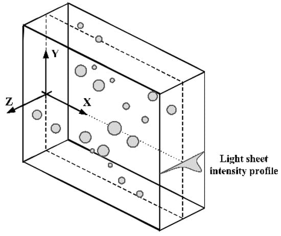
Figure 2.
A three-dimensional volume containing a light sheet and particles, utilized for creating synthetic particle images [13], where particles are represented by gray colored shapes.
The intensity of light sheet can be described as follows [13]:
where represents the efficiency of particle scattering of incident light, denotes the light sheet’s thickness, and is typically set to 2, indicating that the intensity follows a Gaussian distribution.
Although the distribution of the laser along the direction is considered, the synthesized particles still exhibit high peak particle intensity and SNR, leading to an overly idealized image quality that is difficult to replicate under real-world low-SNR conditions. Simulating realistic illumination conditions is complex and impractical. Therefore, we chose to address this issue by focusing on the synthesized images themselves. Specifically, we generated images with varying signal and noise intensities. For signal intensity synthesis, it is important to note that since a large portion of the particles is illuminated by the laser light sheet, we cannot simply reduce the intensity of all particles. Instead, we placed a subset of particles in low-signal-intensity regions, thereby generating synthetic images with mixed signal intensities. To better evaluate the quality of the generated particle images, we define the SNR as
where represents the mean intensity of the signal, and represents the standard deviation of the noise. Considering that our particle images exhibit mixed intensities, with areas of both high-intensity signals and low-intensity signals, the SNR provides an effective method for quantifying image quality. It assesses the clarity and reliability of the image by measuring the prominence of the signal relative to the background noise. The SNR calculated using the above formula reflects the variation in image quality under different noise levels, thus serving as a reference for parameter optimization during the image generation process. The representative synthetic particle images, with their corresponding SNRs generated by our proposed approach, are shown in Figure 3.
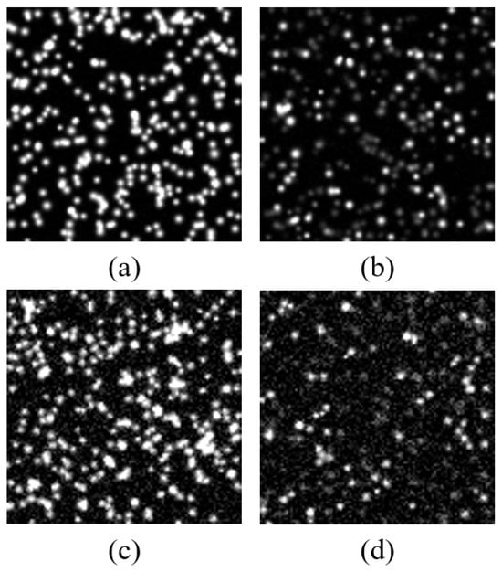
Figure 3.
Synthetic particle images under varying signal strengths and noise levels as follows: (a) high signal strength, low noise, SNR = 20; (b) mixed signal strength, low noise, SNR = 8; (c) mixed signal strength, high noise, SNR = 2; (d) low signal strength, high noise, SNR = 1.
2.2. Training Dataset
Our networks are trained using the synthetic dataset. As shown in Figure 3, the high-noise images with mixed strong and weak signals, generated by the method introduced in Section 2.1, are used as inputs for training, with the corresponding high-signal-strength, low-noise images (i.e., the traditional synthetic particle images) serving as the ground truth. A total of 3000 image pairs are generated for training ED-Net. Similarly, the strong-weak signal-mix low-noise images are used for training CE-Net, with the high-signal-strength, low-noise images (i.e., the traditional synthetic particle images) as the ground truth, again using 6000 image pairs. Finally, high-signal-strength, low-noise images generated with random displacement fields are used for training the RAFT model. The training images are all of size 256 × 256 pixels, and the Particles Per Pixel (PPP) range from 0.1 to 0.4. The structures and functions of these sub-networks are detailed in the following section.
3. PIV-RAFT-EN Algorithm
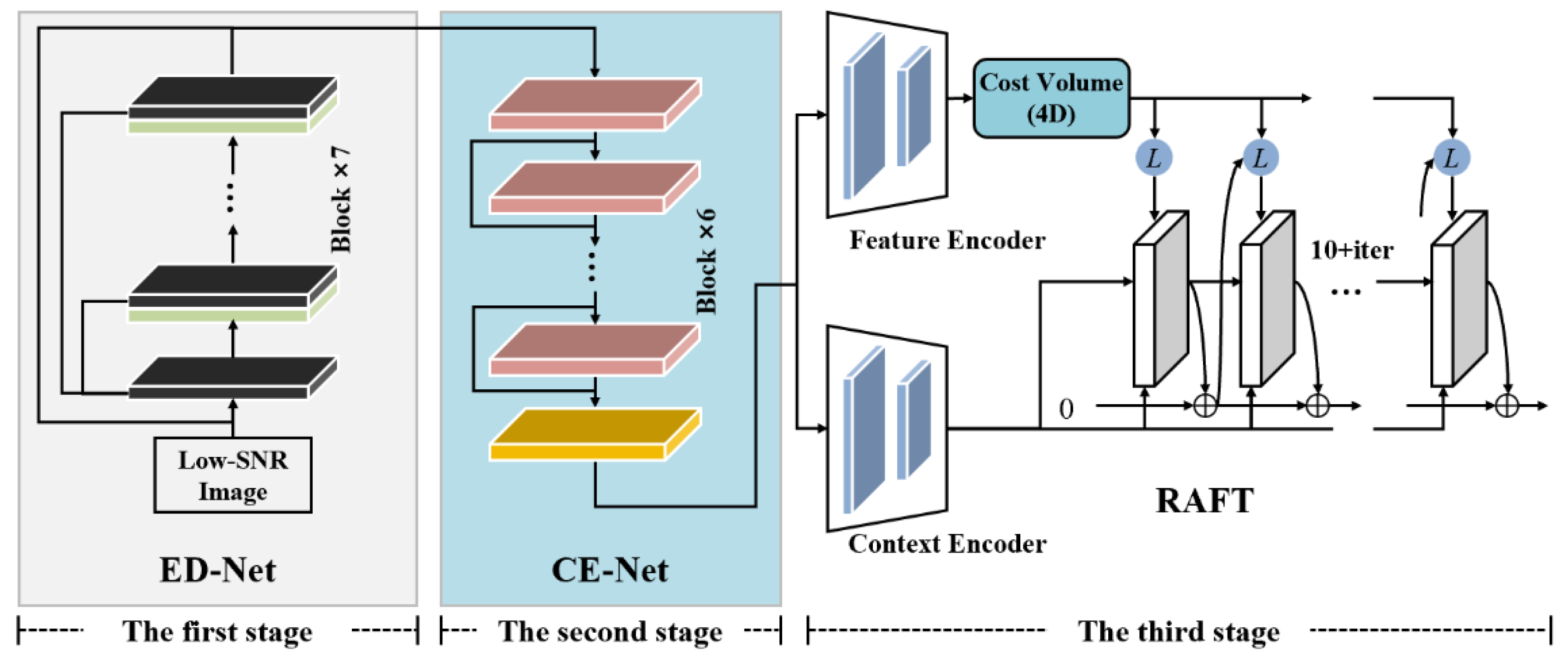
To deal with real-world images characterized by low SNR, we introduce a multi-task convolutional neural network framework named PIV-RAFT-EN. This framework can improve the SNR of images prior to optical flow estimation, thereby enhancing the precision of the prediction. As illustrated in Figure 4, three CNN networks are integrated into PIV-RAFT-EN: ED-Net for image denoising, CE-Net for image contrast enhancement, and the optical flow estimation network RAFT.
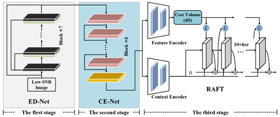
Figure 4.
The overall architecture of PIV-RAFT-EN. PIV-RAFT-EN consists of three stages: ED-Net for edge-enhanced image denoising, CE-Net for contrast enhancement, and RAFT for optical flow estimation. ED-Net incorporates an edge enhancement module and ten convolutional blocks for image denoising. CE-Net comprises nine convolutional layers to extract image features and an adaptive gamma correction module.
3.1. ED-Net
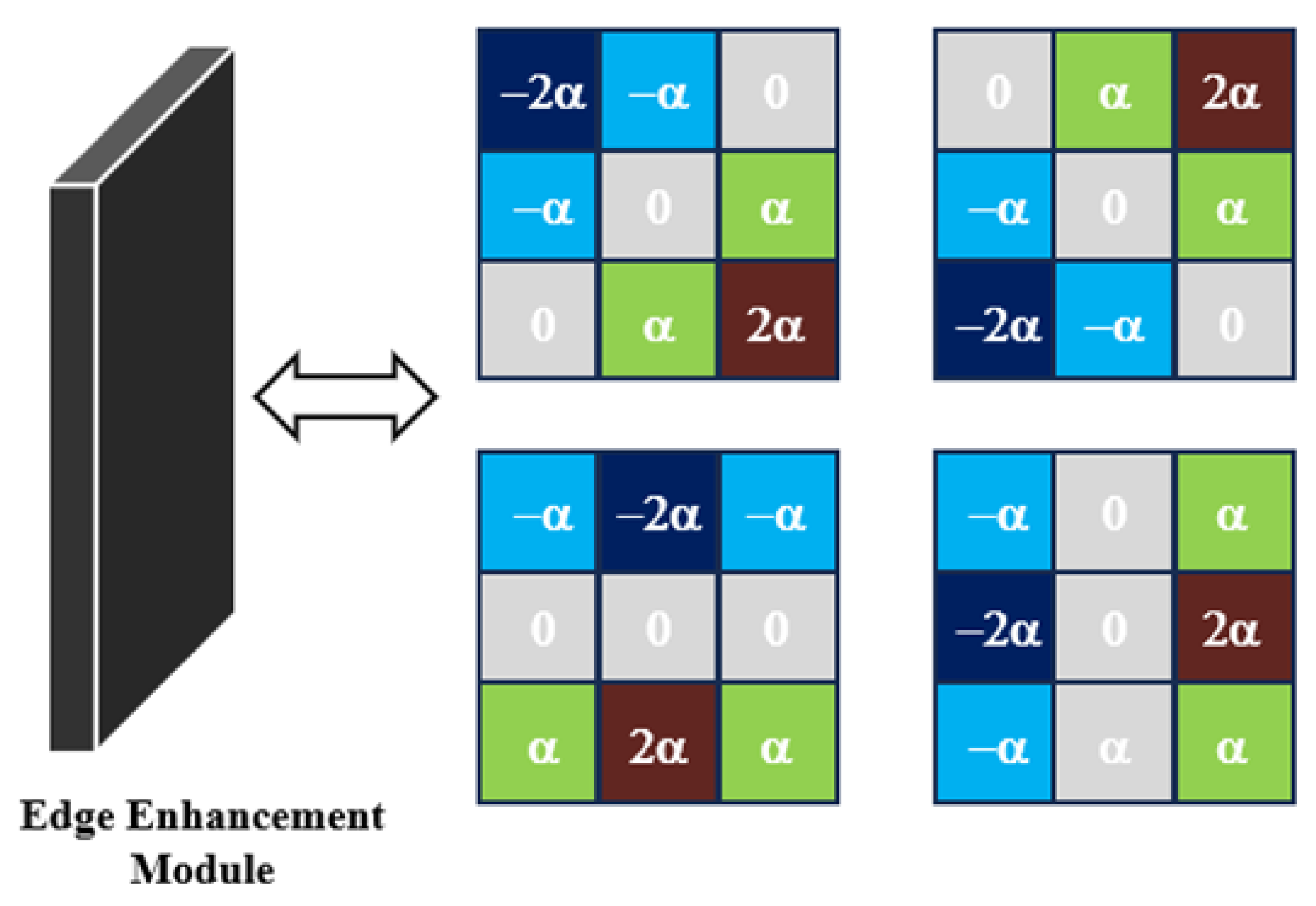
For real-world PIV images characterized by complex background noise and low signal intensity, edge detection is necessary for extracting valuable image features. The Sobel operator is widely used in edge enhancement so that weak signals can be extracted from low SNR images. Unlike traditional fixed-value Sobel operators, a learnable Sobel operator [65,66] is preferred in low SNR image processing, which is illustrated in Figure 5. The factor α can adaptively adjust itself during the optimization and training process and effectively extract edge information with varying intensities.

Figure 5.
The edge enhancement module employs a trainable Sobel kernel for edge feature extraction, where color variations correspond to Sobel kernel parameters.
As shown in Figure 4, the ED-Net network comprises an edge enhancement module and ten convolutional blocks for image denoising. Initially, the input low SNR image is subjected to a set of trainable Sobel convolution operators, resulting in a series of feature maps for edge extraction. Subsequently, these feature maps are concatenated with the input image along the channel dimension to generate the output of the module.
To simplify the task, the model is designed to learn the noise distribution directly. The output of the last convolutional block is summed with the original low SNR image to acquire the final denoised image. After that, by employing a denoising network specially developed for edge enhancement, we can successfully preserve weak signals under low SNR conditions while denoising, which is crucial for the subsequent tasks.
A compound loss function containing a mean square error (MSE) loss and a multiscale perceptual loss is introduced to train ED-Net. To understand the distribution of the noise pixel-wise, the MSE loss function is defined as
where represents the input, represents the target, denotes the denoise model with parameter , and is the number of images. Additionally, a multiscale perceptual loss is employed to avoid excessive smoothing of the output image:
where denotes the model with fixed pre-trained weights for computing the perceptual loss, is the number of images, and is the number of scales. Finally, the compound loss function is defined as follows:
where denotes the hyperparameter that balances the two loss components.
3.2. CE-Net
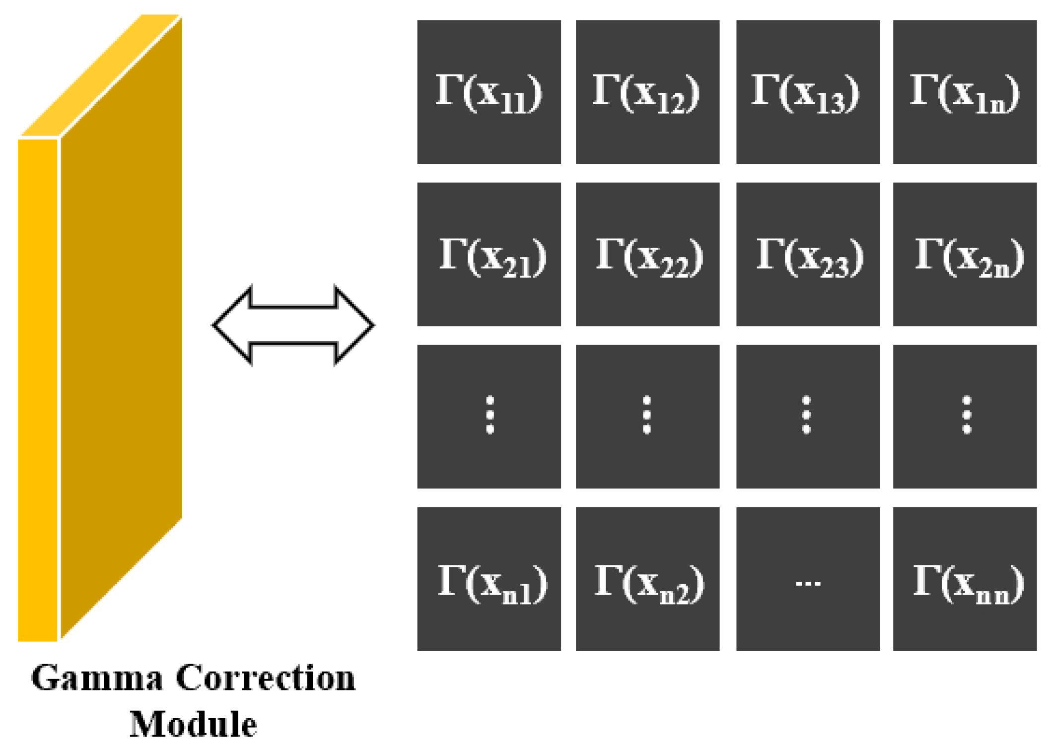
The image denoising network suppresses the non-signal components in the PIV image, but the intensity of the effective signal is still weak. Therefore, an image contrast enhancement network is introduced to increase the intensity of the effective signal. Gamma correction, a widely adopted approach to image contrast enhancement, is also employed in our work. Since this method can brighten underexposed areas with gamma values less than 1 and darken overexposed areas with those greater than 1, selecting an appropriate gamma value is crucial for enhancing image contrast.
This subsection introduces the image contrast enhancement network. As illustrated in Figure 4, this network consists of nine convolutional layers and an adaptive gamma correction module. We input images with low SNR and extract image features through nine convolutional layers, and in the adaptive gamma correction module depicted in Figure 6, a per-pixel gamma mapping has been designed. The gamma correction for each pixel is defined as follows:
where is the original image intensity, and denotes the image intensity after gamma correction.

Figure 6.
The adaptive gamma correction module utilizes a per-pixel gamma mapping for contrast enhancement.
A compound loss function, which incorporates a brightness control loss and an entropy loss , is introduced to train CE-Net. On the one hand, to obtain a more robust enhancement and to suppress excessive luminance gradients between neighboring pixels, we use the maximum value of each window as the pixel value for all pixels in that window instead of using the results of the global gamma transform directly. It can be described as
where is the window around x with the size of 15. Then, the brightness control loss function is defined as
On the other hand, the entropy loss is utilized to increase the global contrast by equalizing the histogram of the output image. Inspired by [67], we designed a soft histogram as follows:
where is the sigmoid function, is the bin width, which is set to 1, and is the hyperparameter. All pixel contributions are summed to obtain a soft histogram for equalization:
Then, we define entropy loss as follows:
Finally, the compound loss function is written as
where denotes the hyperparameter that balances the two loss components.
The input image, which is subjected to the CE-Net based on gamma mapping, demonstrates enhanced contrast and improved quality, thereby facilitating the subsequent optical flow estimation.
3.3. RAFT
RAFT is a state-of-the-art algorithm for optical flow estimation, consisting of three core components: the feature extraction module, correlation calculation layers, and the update iteration module.
As shown in Figure 4, the feature encoder extracts features and from the first and second frame images and maps them to 1/8-resolution feature maps. The feature extraction module is refined to cater to the specific requirements of PIV calculation, maintaining six residual blocks but eliminating the 1/8 down-sampling step. The structures of the context encoder and feature extraction module remain similar, with a focus on extracting contextual information from the first frame. Additionally, a 4D cost volume module is employed to globally match features. This module creates a 4D correlation layer, generating four correlation pyramids to capture both global and local feature information. The correlation query operation is employed to query across four correlation layers, producing feature maps used for subsequent iterative optical flow computation. Next, a Convolutional Gated Recurrent Unit (Conv-GRU) network is used for optical flow computation. Inputs of iterative update operator include outputs of the context encoder, outputs of the cost volume layer, a latent hidden state, and residual flow from previous iterations. At each iteration, the computed residual flow is accumulated with the previous one to generate the current estimation, i.e., . The model adopts the distance as the loss function:
where is set to 0.8 and denotes ground truth flow.
4. Comparisons
This section compares the errors of the PIV-RAFT-EN algorithm with those of Single-Pixel, PIV-RAFT, and window-correlation algorithms using low SNR synthetic images. The results indicate that the PIV-RAFT-EN algorithm outperforms all the other algorithms in accuracy.
4.1. Systematic Errors
The systematic errors of PIV measurements can be divided into two categories: errors caused by experimental hardware conditions, such as crosstalk of the camera and pulse delay of the light source, and errors caused by the PIV algorithm. Assessing the systematic errors caused by the experimental hardware conditions is challenging, whereas the systematic errors caused by the PIV algorithm can be assessed based on the synthesized particle images. Here, the flow in a laminar boundary layer was simulated to assess the systematic errors of PIV-RAFT, PIV-RAFT-EN, Single-Pixel, and window-correlation algorithms.
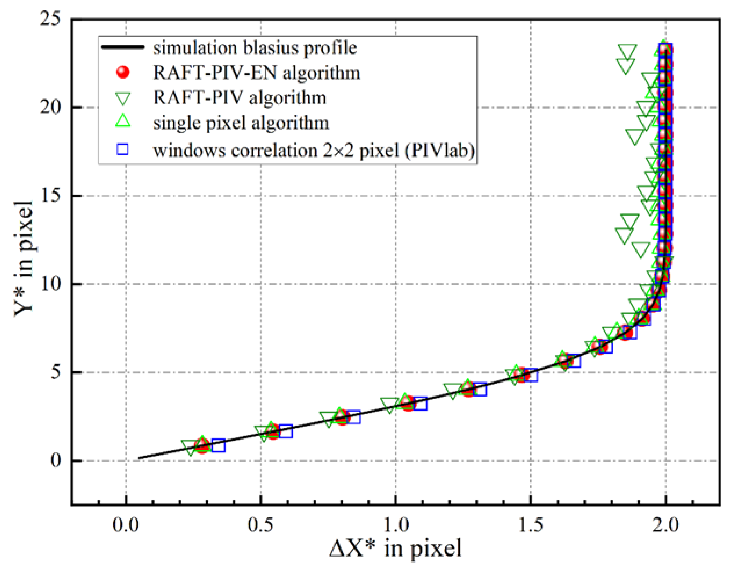
Figure 7 shows the systematic errors of the four algorithms under the condition that the particle diameter D = 3 pixels in the synthesized particle image. The window-correlation method was processed by PIVlab (version 2.63.0.0), with an initial interrogation window size of 32 pixels × 32 pixels and the final size of 2 pixels × 2 pixels. The results indicate that the systematic errors associated with the PIV-RAFT-EN algorithm are lower than those of other algorithms.
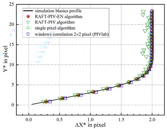
Figure 7.
Comparison of the PIV-RAFT-EN, PIV-RAFT, Single-Pixel, and window-correlation (PIVlab) algorithms within the laminar boundary: profile of the estimated horizontal shift-vector component computed using the four algorithms. The particle image diameter is D = 3 pixels.
4.2. Random Errors
Random errors in PIV measurements come from two sources: experimental conditions and the PIV algorithm. Although the former is difficult to assess due to the random variation of the experimental conditions, the latter can be quantitatively assessed by synthesizing particle images.
We use the standard deviation to describe the random error of the PIV algorithm [13],
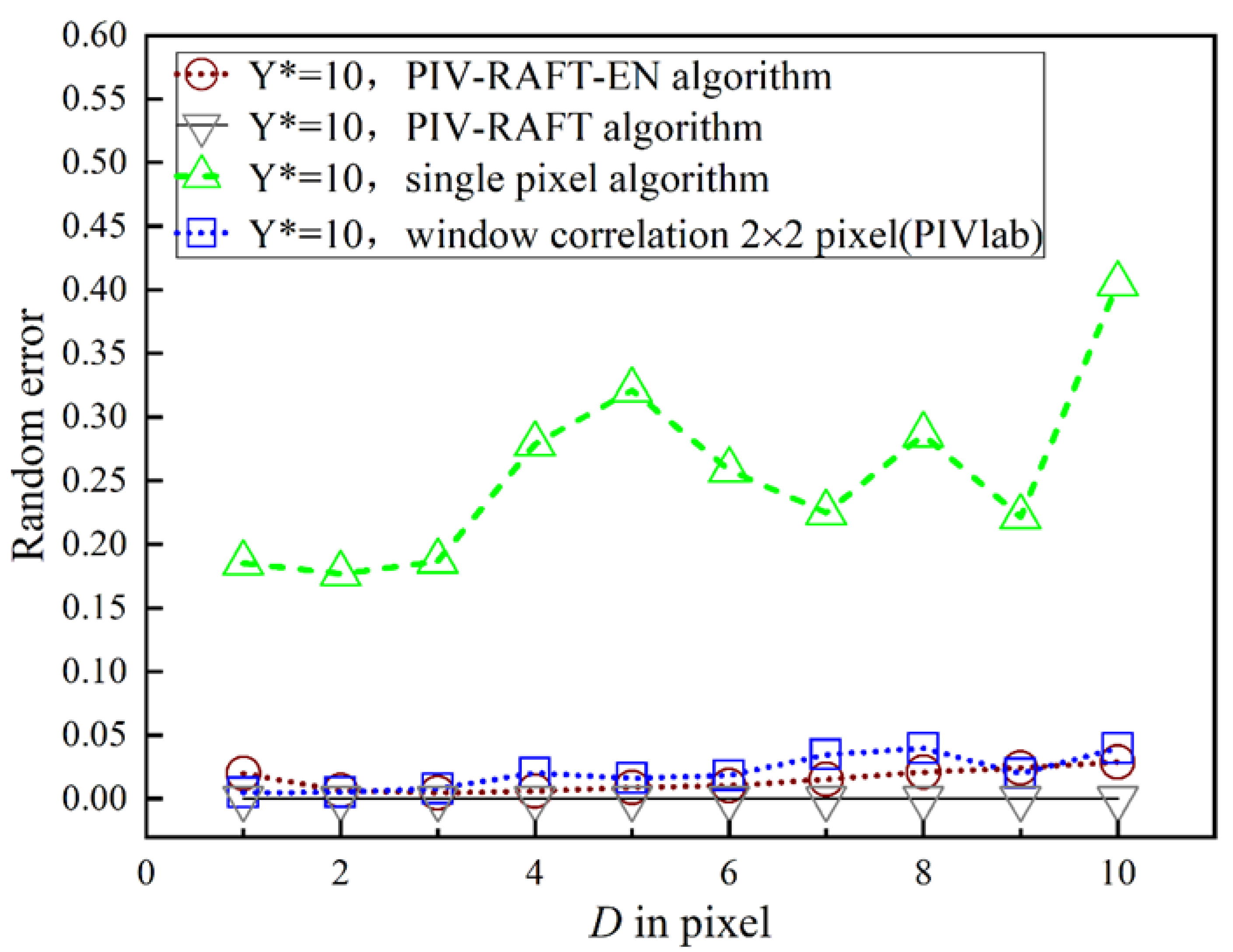
where denotes the number of samples, denotes the individual measured value, and denotes the mean value. Five sets of synthetic particle images (n = 5) were created, each consisting of particles with diameters ranging from 1 pixel to 10 pixels, and 1000 pairs of images were generated for each diameter D.
Figure 8 shows the random errors of the four algorithms at different particle diameters for = 10 pixels. For the majority of cases, the random errors associated with the PIV-RAFT-EN algorithm are lower than those observed in the window-correlation algorithm with 2 pixels × 2 pixels window sizes and the Single-Pixel algorithm. Although PIV-RAFT-EN has slightly higher random errors compared with PIV-RAFT, the systematic errors of PIV-RAFT-EN are significantly lower than those of PIV-RAFT.
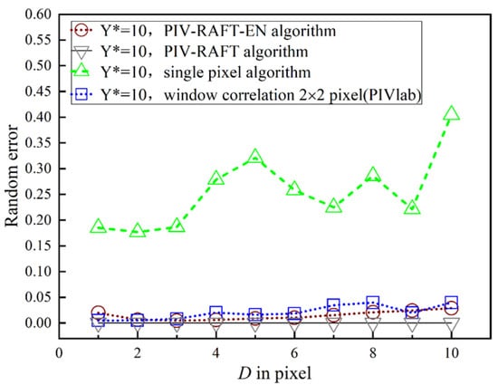
Figure 8.
Comparison of the random errors under the laminar boundary condition.
5. Applications
In this section, by estimating velocity fields from real experimental data of wall-bounded flows, we evaluate the accuracy of four algorithms—PIV-RAFT-EN, PIV-RAFT, Single-Pixel, and window-correlation. The performance of PIV-RAFT-EN was compared with that of other methods to demonstrate its capability in handling real-world images.
5.1. Accurate Measurement of Laminar Flow
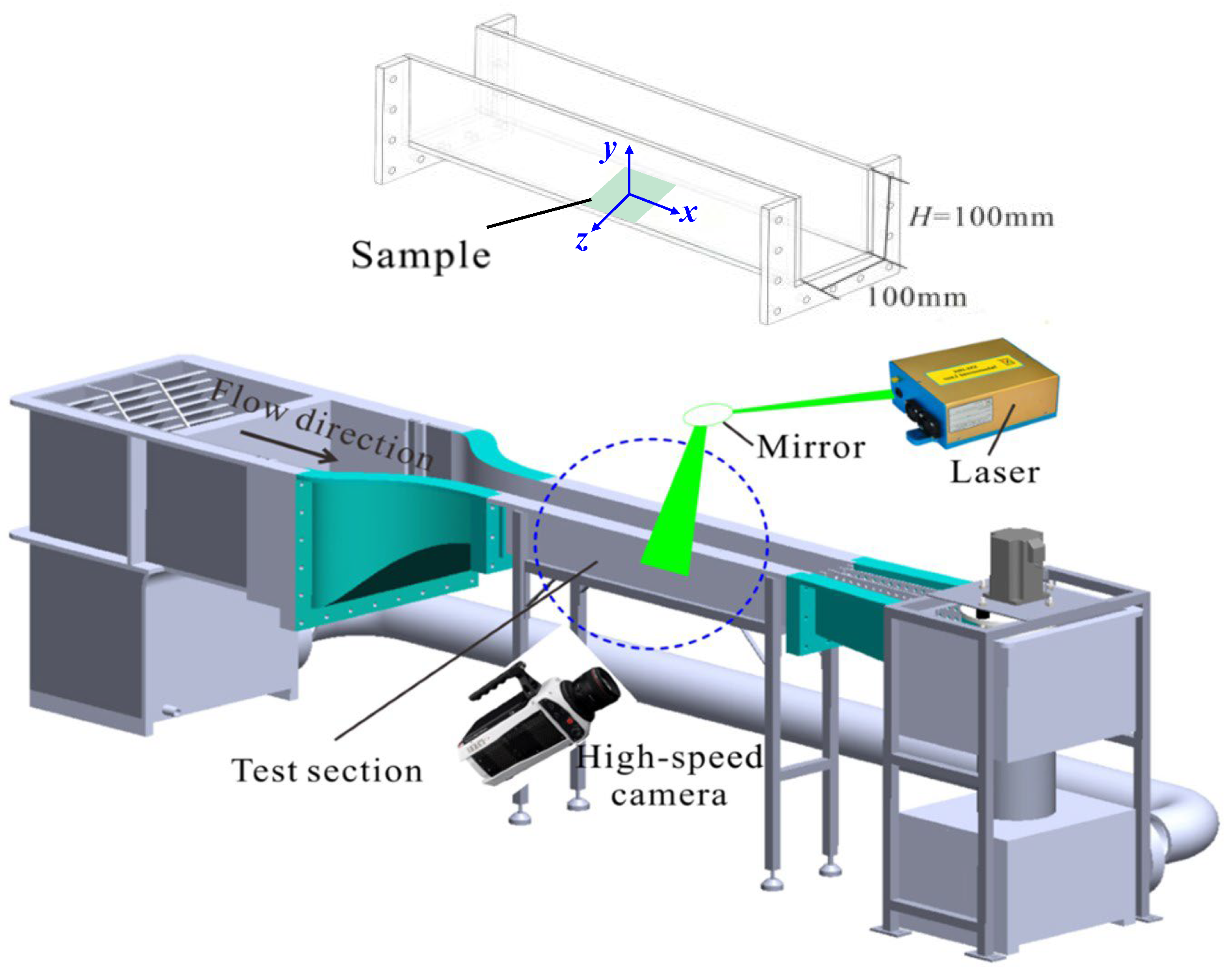
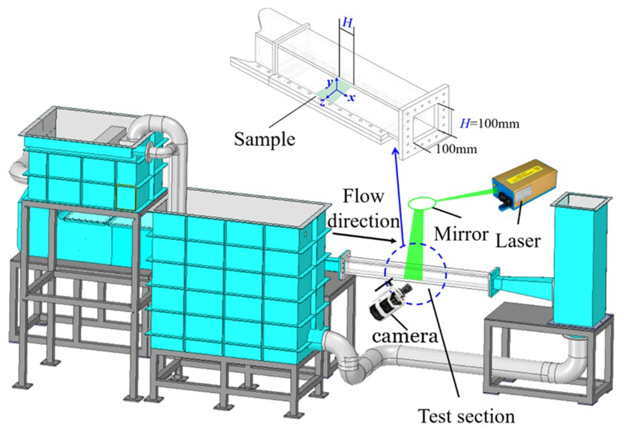
The experiments were conducted in a powered circulating laminar water tank, as shown in Figure 9. The flow was driven by the pump controlled using a variable frequency driver, and then passed through a reservoir, an electromagnetic valve, a stabilization section, and a contraction section before entering the test section. The mean velocity of the inflow, , could be changed by regulating the electromagnetic valve. The test section had a square cross-section with a height of , width of , and a total length of 1200 mm (12H). The walls of the test section were made of transparent acrylic, and the experimental sample was placed on the bottom wall, 800 mm downstream of the tank inlet. The coordinates in the streamwise, spanwise, and wall-normal directions were denoted by , , and , respectively, and the origin was set at the midpoint of the sample, as shown in Figure 9.

Figure 9.
Schematic of the experimental setup, including the circulating laminar water tank facility, the high-speed camera arrangement, and the laser illumination, with the inset showing a zoomed-in view of the test section.
The PIV system is primarily composed of the imaging system and the PIV algorithm. The imaging system includes a high-speed camera (Phantom V2512, Wayne, NJ, USA) with a complementary metal oxide semiconductor (CMOS) sensor of 1080 × 800 pixel2. A macro lens (AT-X PRO 100 mm , Tokina, Nakano, Japan) with an aperture of was used to observe the inner region of the laminar boundary layer (LBL). A continuous laser at 532 nm (LW-HP532-23L, Laserwave, Beijing, China) was utilized to illuminate the water tank. The laser beam was shaped into a sheet of 1 mm through a combination of cylindrical and spherical lenses. The measurement area was 32.5 × 26 mm2, corresponding to a resolution of 1080 × 800 pixel2 on the x–z plane. At least 5000 pairs of particle images were generated at a frequency ranging from 3 kHz to 5 kHz for different . Figure 10 shows a comparison between the near-wall images acquired from the experiments and the low-SNR images we synthesized previously.
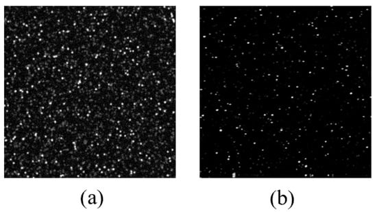
Figure 10.
Comparison of near-wall particle images. (a) Synthetically generated low-SNR particle image.(b) Raw particle image obtained experimentally near the wall.
The aim of this experiment is to investigate the velocity distribution within the laminar boundary layer and to compare the performance of different algorithms in this flow field. The characteristics of the laminar boundary layer result in a velocity profile that follows the typical Blasius solution, where the velocity is zero at the wall and gradually increases to the free-stream velocity as the distance from the wall increases. Given that the velocity distribution in the laminar boundary layer conforms to the classical Blasius solution, it provides an ideal flow field for evaluating the performance of various algorithms, allowing for the assessment of the algorithms in terms of accuracy and spatial resolution.
Based on the experimental images, the local velocity profiles at the plane were calculated using the PIV-RAFT-EN, PIV-RAFT, Single-Pixel algorithm, and window-correlation algorithm. Figure 11 shows the outputs of the individual stages within the PIV-RAFT-EN framework. The window-correlation method was processed with PIVlab, with an initial interrogation window size of 32 pixels × 32 pixels and a final size of 2 pixels × 2 pixels. Both the Single-Pixel and window-correlation algorithms were processed with contrast enhancement and high-pass filtering in PIVlab.
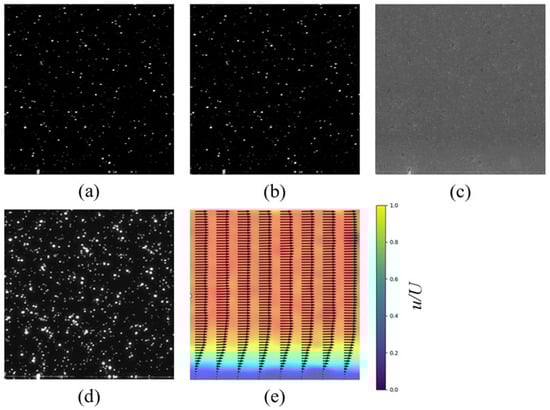
Figure 11.
Stage-wise outputs of the PIV-RAFT-EN algorithm applied to an experimental near-wall image. (a) Input image. (b) Output after ED-Net processing, showing initial noise reduction. (c) Difference image between the ED-Net output and the original input, highlighting the denoising effect. (d) Output after CE-Net processing, demonstrating further signal enhancement. (e) Final output after RAFT model processing, displaying the calculated velocity field as vectors overlaid on a color map representing dimensionless velocity magnitude.
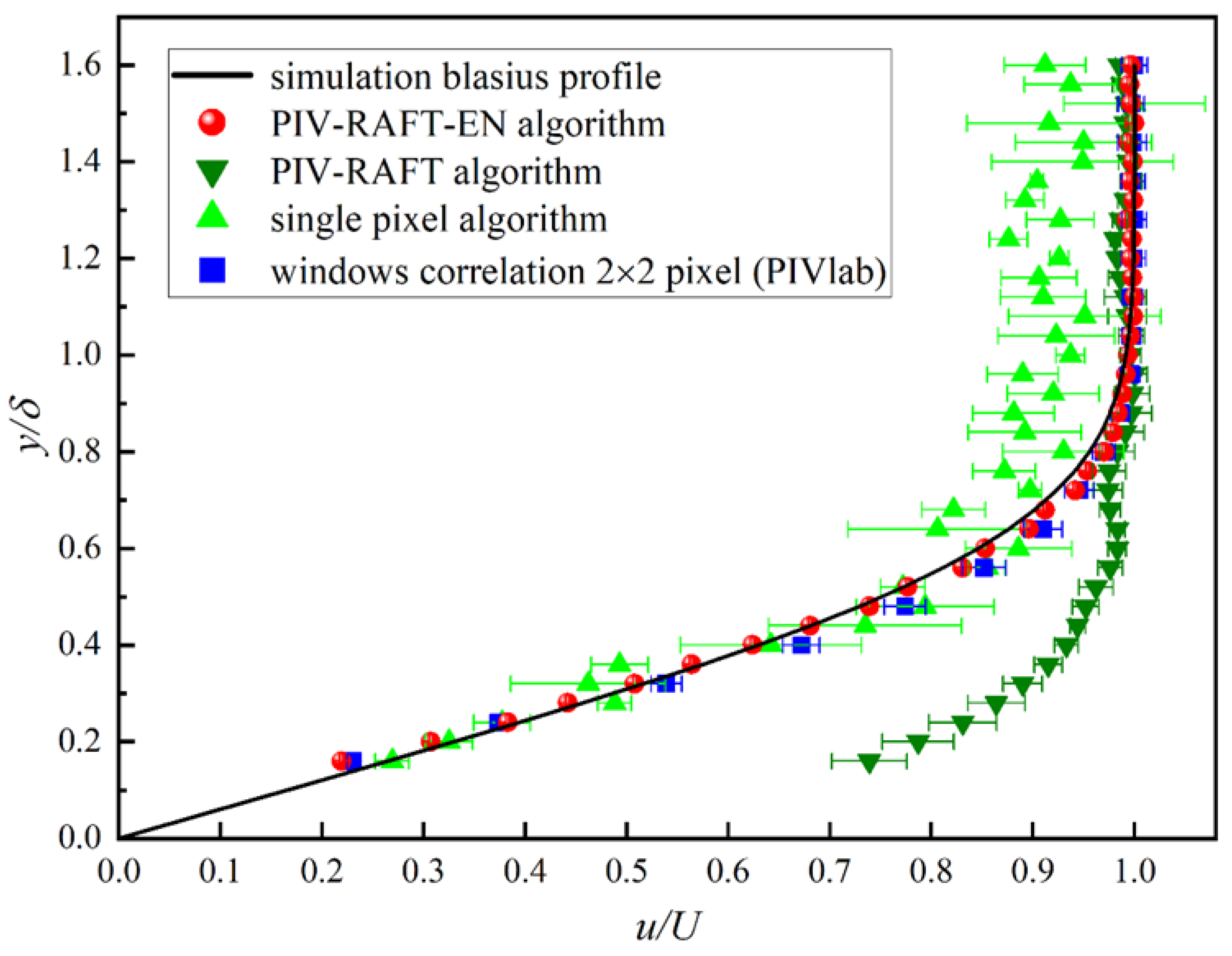
The calculated boundary layer thickness is = 4.5 mm, with a free-stream velocity of = 0.3883 m/s. Figure 12 shows the velocity profiles obtained by these four algorithms, which are plotted in a dimensionless form using the boundary layer thickness and the free-stream velocity for normalization. Specifically, the velocity is normalized as , and the wall-normal coordinate is scaled by . This clearly demonstrates that the results calculated by the PIV-RAFT-EN algorithm and the window-correlation algorithm with a window size of 2 pixels × 2 pixels closely match the Blasius profile, with the PIV-RAFT-EN algorithm demonstrating a higher spatial resolution. In contrast, the PIV-RAFT algorithm and the Single-Pixel algorithm exhibit large error.

Figure 12.
The local velocity profiles near-wall in the plane of calculated by the four PIV algorithms.
5.2. Accurate Measurement on Turbulent Boundary Layer Flow
The experiments were conducted in a gravity-circulating turbulent water tunnel, as shown in Figure 13. To ensure adequate development of the turbulent boundary layer, a 10-mm trip wire was added at the entrance of the experimental section. The test section had a square cross-section with a height of and a width of . The coordinates in the streamwise, spanwise, and wall-normal directions were denoted by , and , respectively, and the origin was set at the midpoint of the sample, as shown in Figure 13. The camera and laser setup are consistent with those described in Section 5.1.

Figure 13.
Schematic of the experimental setup, including the circulating turbulent water tunnel facility, the high-speed camera arrangement, and the laser illumination, with the inset showing a zoomed-in view of the test section.
Based on the experimental images, the local velocity profiles near the wall at the plane were calculated using the PIV-RAFT-EN, PIV-RAFT, Single-Pixel, and window-correlation algorithms. The window-correlation method was processed with PIVlab, with an initial interrogation window size of 32 × 32 pixels and a final size of 2 × 2 pixels. Both the Single-Pixel and window-correlation algorithms were processed with contrast enhancement and high-pass filtering in PIVlab.
The friction velocity for a no-slip smooth surface is given by
where is the wall shear stress and is the fluid density. The wall shear stress is computed as
where is the dynamic viscosity of the fluid and is the velocity gradient in the wall-normal direction of the viscous sublayer.
As shown in Figure 14, the dimensionless velocity is plotted against the dimensionless wall-normal coordinate for different algorithms. Both the velocity and the wall-normal coordinate are non-dimensionalized using the inner scaling of the smooth surface:
where ν is the kinematic viscosity.
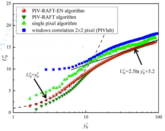
Figure 14.
The local velocity profiles in the turbulent boundary layer at the plane calculated by the four PIV algorithms. The black dashed lines indicate the viscous sublayer, while the black solid lines denote the log-law region.
The dimensionless velocity profile in the viscous sublayer ( < 5) are expected to follow the classic wall law , and in the logarithmic region, the profile can be expressed as
As shown in Figure 14, the accuracy of the PIV-RAFT-EN algorithm is significantly higher than that of the PIV-RAFT, Single-Pixel algorithms, and the window-correlation algorithm. Additionally, the PIV-RAFT-EN algorithm has higher resolution than the window-correlation algorithm and better matches the logarithmic law.
Thus, the PIV-RAFT-EN algorithm demonstrates high accuracy and efficiency in real-world images, particularly in the near-wall regions of wall-bounded flows, where low SNR is typically encountered.
6. Conclusions
In this paper, the PIV-RAFT-EN algorithm has been developed to address the challenges posed by low SNR conditions in PIV measurements. Through systematic comparisons with traditional methods—such as the Single-Pixel, PIV-RAFT, and window-correlation algorithms—using synthetic particle images, PIV-RAFT-EN has been shown to significantly reduce both systematic and random errors while maintaining high spatial resolution. These improvements make the algorithm particularly suitable for environments where image quality is compromised, such as practical applications involving vehicle water ingress.
In addition, the algorithm’s performance has been validated in PIV experiments of laminar and turbulent boundary layers, further confirming its ability to handle real-world low SNR conditions. This performance highlights the robustness of PIV-RAFT-EN for accurate flow field estimation in challenging scenarios where traditional methods often fail to provide reliable results. Given these results, it can be confidently asserted that the PIV-RAFT-EN algorithm holds great promise for various low SNR scenarios, such as marine applications, where accurate flow field data is critical.
In the future, the integration of PIV-RAFT-EN into ocean dynamics research, marine engineering, and environmental monitoring could significantly improve the accuracy and efficiency of flow measurements in dynamic and complex marine environments. Furthermore, the potential of the algorithm for use in real-time applications, such as vehicle water intrusion analysis and underwater robotics, opens up avenues for further research and practical applications in the field of marine science. Thus, this work not only contributes to the advancement of PIV technology but also lays the foundation for future applications in complex environmental and engineering systems.
Author Contributions
Software, Y.W.; Investigation, Y.W.; Resources, C.Y. and D.P.; Data curation, D.P.; Writing—original draft, P.L.; Supervision, H.L.; Funding acquisition, H.L. All authors have read and agreed to the published version of the manuscript.
Funding
This paper was supported by the National Natural Science Foundation of China (NSFC) under Grant Nos. 12202010, 52461045, 12293001, U2141251, the Beijing Nova Program (20240484719), the Laoshan Laboratory (Grant No. LSKJ202200500), and the National Key R&D Program of China (2022YFC2806604). The APC was supported by the Beijing Nova Program (20240484719).
Data Availability Statement
The raw data supporting the conclusions of this article will be made available by the authors on request.
Conflicts of Interest
The authors declare no conflict of interest.
References
- Oldenziel, G.; Sridharan, S.; Westerweel, J. Measurement of high-Re turbulent pipe flow using Single-Pixel PIV. Exp. Fluids 2023, 64, 164. [Google Scholar] [CrossRef]
- Chau, T.V.; Jung, S.; Kim, M.; Na, W.-B. Analysis of the Bending Height of Flexible Marine Vegetation. J. Mar. Sci. Eng. 2024, 12, 1054. [Google Scholar] [CrossRef]
- Chen, S.; Zhang, Y.; Su, T.; Gong, Y. PIV Experimental Research and Numerical Simulation of the Pigging Process. J. Mar. Sci. Eng. 2024, 12, 549. [Google Scholar] [CrossRef]
- D’Agostino, D.; Diez, M.; Felli, M.; Serani, A. PIV Snapshot Clustering Reveals the Dual Deterministic and Chaotic Nature of Propeller Wakes at Macro- and Micro-Scales. J. Mar. Sci. Eng. 2023, 11, 1220. [Google Scholar] [CrossRef]
- He, T.; Hu, H.; Tang, D.; Chen, X.; Meng, J.; Cao, Y.; Lv, X. Experimental Study on the Effects of Waves and Current on Ice Melting. J. Mar. Sci. Eng. 2023, 11, 1209. [Google Scholar] [CrossRef]
- Lin, Y.-T.; Liu, L.; Sheng, B.; Yuan, Y.; Hu, K. Laboratory Studies of Internal Solitary Waves Propagating and Breaking over Submarine Canyons. J. Mar. Sci. Eng. 2023, 11, 355. [Google Scholar] [CrossRef]
- Le, A.V.; Fenech, M. Image-Based Experimental Measurement Techniques to Characterize Velocity Fields in Blood Microflows. Front Physiol. 2022, 13, 886675. [Google Scholar] [CrossRef]
- Liu, L.; Zhao, L.; Wang, Y.; Zhang, S.; Song, M.; Huang, X.; Lu, Z. Research on the Enhancement of the Separation Efficiency for Discrete Phases Based on Mini Hydrocyclone. J. Mar. Sci. Eng. 2022, 10, 1606. [Google Scholar] [CrossRef]
- Meng, Z.; Zhang, J.; Hu, Y.; Ancey, C. Temporal Prediction of Landslide-Generated Waves Using a Theoretical–Statistical Combined Method. J. Mar. Sci. Eng. 2023, 11, 1151. [Google Scholar] [CrossRef]
- Ning, C.; Li, Y.; Huang, P.; Shi, H.; Sun, H. Numerical Analysis of Single-Particle Motion Using CFD-DEM in Varying-Curvature Elbows. J. Mar. Sci. Eng. 2022, 10, 62. [Google Scholar] [CrossRef]
- Orzech, M.; Yu, J.; Wang, D.; Landry, B.; Zuniga-Zamalloa, C.; Braithwaite, E.; Trubac, K.; Gray, C. Laboratory Measurements of Surface Wave Propagation through Ice Floes in Salt Water. J. Mar. Sci. Eng. 2022, 10, 1483. [Google Scholar] [CrossRef]
- Adrian, R.J.; Westerweel, J. Particle Image Velocimetry; Cambridge University Press: Cambridge, MA, USA, 2011. [Google Scholar]
- Raffel, M.; Willert, C.E.; Scarano, F.; Kähler, C.J.; Wereley, S.T.; Kompenhans, J. Particle Image Velocimetry: A Practical Guide; Springer: Berlin, Germany, 2018. [Google Scholar]
- Wereley, S.T.; Gui, L.; Meinhart, C. Advanced algorithms for microscale particle image velocimetry. AIAA J. 2002, 40, 1047–1055. [Google Scholar] [CrossRef]
- Kaehler, C.J.; Scharnowski, S.; Cierpka, C. On the uncertainty of digital PIV and PTV near walls. Exp. Fluids 2012, 52, 1641–1656. [Google Scholar] [CrossRef]
- Gao, Z.; Li, X.; Ye, H. Aberration correction for flow velocity measurements using deep convolutional neural networks. Infrared Laser Eng. 2020, 49, 20200267. [Google Scholar]
- Weng, W.; Fan, W.; Liao, G.; Qin, J. Wavelet-based image denoising in (digital) particle image velocimetry. Signal Process. 2001, 81, 1503–1512. [Google Scholar] [CrossRef]
- Adatrao, S.; Sciacchitano, A. Elimination of unsteady background reflections in PIV images by anisotropic diffusion. Meas. Sci. Technol. 2019, 30, 035204. [Google Scholar] [CrossRef]
- Grayson, K.; de Silva, C.M.; Hutchins, N.; Marusic, I. Impact of mismatched and misaligned laser light sheet profiles on PIV performance. Exp. Fluids 2018, 59, 2. [Google Scholar] [CrossRef]
- Wang, L.; Pan, C.; Liu, J.; Cai, C. Ratio-cut background removal method and its application in near-wall PTV measurement of a turbulent boundary layer. Meas. Sci. Technol. 2021, 32, 25302. [Google Scholar] [CrossRef]
- Theunissen, R.; Scarano, F.; Riethmuller, M. On improvement of PIV image interrogation near stationary interfaces. Exp. Fluids 2008, 45, 557–572. [Google Scholar] [CrossRef]
- Raben, J.S.; Hariharan, P.; Robinson, R.; Malinauskas, R.; Vlachos, P.P. Time-resolved particle image velocimetry measurements with wall shear stress and uncertainty quantification for the FDA nozzle model. Cardiovasc. Eng. Technol. 2016, 7, 7–22. [Google Scholar] [CrossRef]
- Becker, F.; Wieneke, B.; Petra, S.; Schroder, A.; Schnorr, C. Variational adaptive correlation method for flow estimation. IEEE Trans Image Process. 2011, 21, 3053–3065. [Google Scholar] [CrossRef] [PubMed]
- Scharnowski, S.; Kaehler, C.J. Particle image velocimetry—Classical operating rules from today’s perspective. Opt. Lasers Eng. 2020, 135, 106185. [Google Scholar] [CrossRef]
- Yu, C.; Bi, X.; Fan, Y. Deep learning for fluid velocity field estimation: A review. Ocean Eng. 2023, 271, 113693. [Google Scholar] [CrossRef]
- Wereley, S.T.; Meinhart, C.D. Second-order accurate particle image velocimetry. Exp. Fluids 2001, 31, 258–268. [Google Scholar] [CrossRef]
- Wieneke, B.; Pfeiffer, K. Adaptive PIV with variable interrogation window size and shape. In Proceedings of the 15th International Symposium on Applications of Laser Techniques to Fluid Mechanics, Lisbon, Portugal, 5–8 July 2010. [Google Scholar]
- Kaehler, C.J.; Scharnowski, S.; Cierpka, C. On the resolution limit of digital particle image velocimetry. Exp. Fluids 2012, 52, 1629–1639. [Google Scholar] [CrossRef]
- Theunissen, R.; Scarano, F.; Riethmuller, M.L. Spatially adaptive PIV interrogation based on data ensemble. Exp. Fluids 2010, 48, 875–887. [Google Scholar] [CrossRef]
- Scarano, F. Iterative image deformation methods in PIV. Meas. Sci. Technol. 2001, 13, R1. [Google Scholar] [CrossRef]
- Westerweel, J.; Scarano, F. Universal outlier detection for PIV data. Exp. Fluids 2005, 39, 1096–1100. [Google Scholar] [CrossRef]
- Stanislas, M.; Abdelsalam, D.G.; Coudert, S. CCD camera response to diffraction patterns simulating particle images. Appl. Optics 2013, 52, 4715–4723. [Google Scholar] [CrossRef]
- Theunissen, R.; Scarano, F.; Riethmuller, M.L. An adaptive sampling and windowing interrogation method in PIV. Meas. Sci. Technol. 2006, 18, 275. [Google Scholar] [CrossRef]
- Xie, Z.; Wang, H.; Xu, D. Spatiotemporal optimization on cross correlation for particle image velocimetry. Phys. Fluids 2022, 34, 55105. [Google Scholar] [CrossRef]
- Westerweel, J.; Poelma, C.; Lindken, R. Two-point ensemble correlation method for µPIV applications. In Proceedings of the 11th International Symposium on ‘Applications of Laser Techniques to Fluid Mechanics, Lisbon, Portugal, 8–11 July 2002. [Google Scholar]
- Westerweel, J.; Geelhoed, P.F.; Lindken, R. Single-Pixel resolution ensemble correlation for micro-PIV applications. Exp. Fluids 2004, 37, 375–384. [Google Scholar] [CrossRef]
- Li, H.; Cao, Y.; Wang, X.; Wan, X.; Xiang, Y.; Yuan, H.; Lv, P.; Duan, H. Accurate PIV measurement on slip boundary using Single-Pixel algorithm. Meas. Sci. Technol. 2022, 33, 55302. [Google Scholar] [CrossRef]
- Chuang, H.-S.; Gui, L.; Wereley, S.T. Nano-resolution flow measurement based on single pixel evaluation PIV. Microfluid. Nanofluid. 2012, 13, 49–64. [Google Scholar] [CrossRef]
- Karchevskiy, M.N.; Tokarev, M.P.; Yagodnitsyna, A.A.; Kozinkin, L.A. Correlation algorithm for computing the velocity fields in microchannel flows with high resolution. Thermophys. Aeromechanics 2015, 22, 745–754. [Google Scholar] [CrossRef]
- Corpetti, T.; Heitz, D.; Arroyo, G.; Mémin, E.; Santa-Cruz, A. Fluid experimental flow estimation based on an optical-flow scheme. Exp. Fluids 2006, 40, 80–97. [Google Scholar] [CrossRef]
- Horn, B.K.; Schunck, B.G. Determining optical flow. Artif. Intell. 1981, 17, 185–203. [Google Scholar] [CrossRef]
- Wang, B.; Cai, Z.; Shen, L.; Liu, T. An analysis of physics-based optical flow. J. Comput. Appl. Math. 2015, 276, 62–80. [Google Scholar] [CrossRef]
- Khalid, M.; Pénard, L.; Mémin, E. Optical flow for image-based river velocity estimation. Flow Meas. Instrum. 2019, 65, 110–121. [Google Scholar] [CrossRef]
- Chen, J.; Duan, H.; Song, Y.; Cai, Z.; Yang, G.; Liu, T. Motion estimation for complex fluid flows using Helmholtz decomposition. IEEE Trans. Circuits Syst. Video Technol. 2022, 33, 2129–2146. [Google Scholar] [CrossRef]
- Yang, Z.; Johnson, M. Hybrid particle image velocimetry with the combination of cross-correlation and optical flow method J. Vis. 2017, 20, 625–638. [Google Scholar] [CrossRef]
- Liu, T. OpenOpticalFlow: An open source program for extraction of velocity fields from flow visualization images. J. Open Res. Softw. 2017, 5, 29. [Google Scholar] [CrossRef]
- Tao, W.; Liu, Y.; Ma, Z.; Hu, W. Two-Dimensional Flow Field Measurement Method for Sediment-Laden Flow Based on Optical Flow Algorithm. Appl. Sci. 2022, 12, 2720. [Google Scholar] [CrossRef]
- Ruhnau, P.; Stahl, A.; Schnörr, C. Variational estimation of experimental fluid flows with physics-based spatio-temporal regularization. Meas. Sci. Technol. 2007, 18, 755. [Google Scholar] [CrossRef]
- Schmidt, B.; Sutton, J. Improvements in the accuracy of wavelet-based optical flow velocimetry (wOFV) using an efficient and physically based implementation of velocity regularization. Exp. Fluids 2020, 61, 1–17. [Google Scholar] [CrossRef]
- Cassisa, C.; Simoens, S.; Prinet, V.; Shao, L. Subgrid scale formulation of optical flow for the study of turbulent flow. Exp. Fluids 2011, 51, 1739–1754. [Google Scholar] [CrossRef]
- Alvarez, L.; Castaño, C.; García, M.; Krissian, K.; Mazorra, L.; Salgado, A.; Sánchez, J. Variational second order flow estimation for PIV sequences. Exp. Fluids 2008, 44, 291–304. [Google Scholar] [CrossRef]
- Zhong, Q.; Yang, H.; Yin, Z. An optical flow algorithm based on gradient constancy assumption for PIV image processing. Meas. Sci. Technol. 2017, 28, 55208. [Google Scholar] [CrossRef]
- Liu, T.; Merat, A.; Makhmalbaf, M.; Fajardo, C.; Merati, P. Comparison between optical flow and cross-correlation methods for extraction of velocity fields from particle images. Exp. Fluids 2015, 56, 1–23. [Google Scholar] [CrossRef]
- Rabault, J.; Kolaas, J.; Jensen, A. Performing particle image velocimetry using artificial neural networks: A proof-of-concept. Meas. Sci. Technol. 2017, 28, 125301. [Google Scholar] [CrossRef]
- Lee, Y.; Yang, H.; Yin, Z. PIV-DCNN: Cascaded deep convolutional neural networks for particle image velocimetry. Exp. Fluids 2017, 58, 171. [Google Scholar] [CrossRef]
- Dosovitskiy, A.; Fischer, P.; Ilg, E.; Hausser, P.; Hazirbas, C.; Golkov, V.; Van Der Smagt, P.; Cremers, D.; Brox, T. Flownet: Learning optical flow with convolutional networks. In Proceedings of the IEEE International Conference on Computer Vision, Santiago, Chile, 7–13 December 2015. [Google Scholar]
- Ilg, E.; Mayer, N.; Saikia, T.; Keuper, M.; Dosovitskiy, A.; Brox, T. Flownet 2.0: Evolution of optical flow estimation with deep networks. In Proceedings of the IEEE Conference on Computer Vision and Pattern Recognition, Honolulu, HI, USA, 21–26 July 2017. [Google Scholar]
- Hui, T.-W.; Tang, X.; Loy, C.C. Liteflownet: A lightweight convolutional neural network for optical flow estimation. In Proceedings of the 2018 IEEE/CVF Conference on Computer Vision and Pattern Recognition (CVPR 2018), Salt Lake City, UT, USA, 18–22 June 2018. [Google Scholar]
- Sun, D.; Yang, X.; Liu, M.-Y.; Kautz, J. Pwc-net: Cnns for optical flow using pyramid, warping, and cost volume. In Proceedings of the 2018 IEEE/CVF Conference on Computer Vision and Pattern Recognition (CVPR), Salt Lake City, UT, USA, 18–23 June 2018. [Google Scholar]
- Teed, Z.; Deng, J. Raft: Recurrent all-pairs field transforms for optical flow. In Proceedings of the ECCV European Conference on Computer Vision (ECCV 2020), Glasgow, UK, 23–28 August 2020. [Google Scholar]
- Yu, C.; Bi, X.; Fan, Y.; Han, Y.; Kuai, Y. LightPIVNet: An Effective Convolutional Neural Network for Particle Image Velocimetry. IEEE Trans. Instrum. Meas. 2021, 70, 1–15. [Google Scholar] [CrossRef]
- Han, Y.; Wang, Q. An attention-mechanism incorporated deep recurrent optical flow network for particle image velocimetry. Phys. Fluids 2023, 35, 75122. [Google Scholar]
- Lagemann, C.; Lagemann, K.; Mukherjee, S.; Schroder, W. Deep recurrent optical flow learning for particle image velocimetry data. Nat. Mach. Intell. 2021, 3, 641–651. [Google Scholar] [CrossRef]
- Lagemann, C.; Lagemann, K.; Mukherjee, S.; Schroder, W. Generalization of deep recurrent optical flow estimation for particle-image velocimetry data. Meas. Sci. Technol. 2022, 33, 94003. [Google Scholar] [CrossRef]
- Liang, T.; Jin, Y.; Li, Y.; Wang, T. Edcnn: Edge enhancement-based densely connected network with compound loss for low-dose ct denoising. In Proceedings of the 2020 15th IEEE International Conference on Signal Processing (ICSP), Beijing, China, 18–22 October 2020. [Google Scholar]
- Luthra, A.; Sulakhe, H.; Mittal, T.; Iyer, A.; Yadav, S. Eformer: Edge Enhancement based Transformer for Medical Image Denoising. arXiv 2021, arXiv:2109.08044. [Google Scholar]
- Alivanoglou, A.; Likas, A. Probabilistic models based on the π-sigmoid distribution. In Proceedings of the Artificial Neural Networks in Pattern Recognition: Third IAPR Workshop, ANNPR 2008, Paris, France, 2–4 July 2008. Proceedings 3. [Google Scholar]


Disclaimer/Publisher’s Note: The statements, opinions and data contained in all publications are solely those of the individual author(s) and contributor(s) and not of MDPI and/or the editor(s). MDPI and/or the editor(s) disclaim responsibility for any injury to people or property resulting from any ideas, methods, instructions or products referred to in the content. |
© 2025 by the authors. Licensee MDPI, Basel, Switzerland. This article is an open access article distributed under the terms and conditions of the Creative Commons Attribution (CC BY) license (https://creativecommons.org/licenses/by/4.0/).