Characteristics and Rapid Prediction of Seismic Subsidence of Saturated Seabed Foundation with Interbedded Soft Clay–Sand

Abstract

Seabed foundations consisting of interbedded layers of saturated soft clay and sand deposited during the Quaternary period are widely distributed in the coastal areas of Southeastern China. These soil foundations are prone to significant settlement under seismic loading. The study of the seismic dynamic response characteristics of saturated foundations with interbedded soft clay–sand and the development of rapid prediction models are essential for controlling settlement and ensuring the service safety of marine structures. A total of 4000 sets of seabed foundation models are randomly generated, with layers of saturated soft clay and sand and with a random distribution of layer thickness and burial depth. The mechanical behavior of saturated soft clay is described using the Soft Clay model based on the boundary surface theory, and the generalized elastoplastic constitutive model PZIII is used to characterize the mechanical behavior of sandy soil. The finite element platform FssiCAS is employed for a computational analysis to study the characteristics of seismic subsidence in saturated seabed foundations with interbedded soft clay–sand. A machine learning model is implemented based on the Random Forest algorithm, in which 3200 sets of numerical simulation results are used for model training, and 800 sets are used for validating the model’s reliability. The results show that under seismic excitation, the pore water pressure within the saturated seabed foundation with interbedded soft clay–sand accumulates, effective stress decreases, and the seabed foundation softens, to a certain extent. During the post-seismic consolidation phase, significant settlement of the seabed foundation occurs. The fast prediction model based on the Random Forest algorithm could reliably predict the settlement characteristics of submarine foundations. This research provides a new technological avenue for the rapid prediction of the seismic settlement of submarine foundations, which could be of use in engineering design, assessment, and prediction.

1. Introduction

Driven by marine economic expansion, a large array of marine infrastructure has been built in the southeast coastal areas of China [1], such as offshore wind turbines, submarine oil pipelines, offshore exploration and construction platforms, and so on. Quaternary sedimentary saturated seabed foundations with interbedded soft clay–sand are extensively distributed in the coastal areas of Southeastern China. The mechanical properties of seabed foundations are unstable [2], and large-scale settlements easily occur under seismic loads. Research on the seismic dynamic response characteristics of saturated foundations with interbedded soft clay–sand and the rapid prediction of their settlement are of great significance for controlling settlement and ensuring the service safety of marine structures.

In recent decades, many scholars both domestically and internationally have studied the response characteristics of soils under seismic loading using methods such as geotechnical testing and numerical simulation. In experimental studies, Zhang et al. [3], Zhou et al. [4], and Li et al. [5] demonstrated that under strong seismic loading conditions in which drainage paths are extended or drainage is impeded, progressive pore pressure accumulation may lead to liquefaction phenomena, particularly in loose sand seabed foundations. This observation is corroborated by Manika et al. [6], Yosuke Higo et al. [7], and Pradipta et al. [8], who observed that under seismic loading, significant pore pressure accumulation occurs in loose sand foundations, with the excess pore pressure being notably high. In experimental studies on the characteristics of soft soil seismic subsidence, Yu et al. [9] demonstrated that under the action of vibratory loading, saturated soft soil cannot drain in time, resulting in the effective stress in the soil being converted into pore water pressure, which leads to a reduction in the deformation modulus of the soil and softening of the soil. Xie et al. [10] found through shaking table experiments that sand liquefaction is influenced by peak ground acceleration (PGA) and seismic wave frequency, with high-frequency seismic waves being more likely to induce sand liquefaction.

As for numerical simulations, Vasiliki et al. [11] used the finite element method to find that the additional plastic deformation of saturated sand caused by vertical ground motion increases the liquefaction depth and trigger time. By simulating the seismic response of submarine breakwater, Gu et al. [12] found that the pore water pressure dissipation and consolidation duration of a thick clay foundation is longer than that of a sand foundation. Using an OpenSees V2.4 analysis, Gu et al. [13] found that the peak acceleration and frequency spectrum characteristics of ground motion have a significant influence on the seismic subsidence of soft soil. Gao et al. [14] established a three-dimensional analysis model of sand based on Abaqus to simulate the influence of relative density and clay content on the seismic subsidence of sand under different seismic wave loads. Gao et al. [15] investigated the behavior of suction bucket foundations in liquefiable sand under seismic action, revealing the threat of foundation liquefaction to the safety of suction bucket foundations. Chen et al. [16] investigated the significant influence of the peak seismic wave amplification effect on the seismic response of a monopile–water–foundation-coupled system.

Of the numerical simulation studies mentioned above, many of them have used elastic models or idealized elasto-plastic constitutive models to describe the dynamic response behavior of seabed soils. However, these models are unable to accurately capture key features such as the dynamic softening and liquefaction of marine soft ground. Therefore, the reliability of these numerical simulation studies in analyzing the dynamic response characteristics of submarine foundations is insufficient.

Ye et al. [17] established a coupled numerical model, FssiCAS, which integrates the RAVANS equations controlling wave and pore flow and Biot’s equations controlling the dynamic response of the structure and subsea foundations and contains a relatively complete constitutive model of the seabed foundation soils. The predictive accuracy of the numerical model FssiCAS has been widely verified [18] by experimental tests and analytical solutions. Currently, FssiCAS has been effectively employed in offshore structural stability analysis and consolidation settlement prediction [18], offshore wave–structure–seabed response analysis [19], and the nonlinear dynamic response of shallow buried pipelines under wave action [20]. It should be noted that numerical simulation involves processes such as geometric modelling, meshing, boundary conditions, and solution calculations. It is acceptable to carry out a numerical simulation once or several times, but if the working conditions are particularly numerous, corresponding to hundreds or thousands of cases, then it is obviously not currently feasible to carry out a numerical simulation for each working condition. In practical engineering, a fast solution method is required. Machine learning can be a good solution to this problem.

Currently, machine learning algorithms have been widely recognized by researchers at home and abroad in the field of geotechnical engineering. Zhao et al. [21] were the first to successfully use the Support Vector Machine (SVM) algorithm to predict the settlement of soft soil foundations in highways. The model they developed effectively represented the mapping relationship between settlement and other factors, demonstrating a high degree of accuracy and strong generalization capability. Subsequently, Chen et al. [22] optimized the training parameters of the SVM using the Ant Colony Optimization (ACO) algorithm, further improving the SVM’s precision and successfully applying it to tunnel settlement prediction. However, Chen failed to comprehensively investigate the influence of certain parameters during the application of the model. To reduce the impact of some influencing factors on the prediction accuracy of machine learning, Ling et al. [23] employed the more robust Random Forest algorithm to predict surface settlement in subway tunnels. Wang et al. [24] combined the Random Forest algorithm with SVM, using the Random Forest algorithm to eliminate redundant variables, and then applied the data with reduced dimensions to establish an SVM model to predict building settlement during tunnel shield construction. Although these studies have proven the applicability of machine learning in soil settlement prediction, they have certain limitations when extended to seismic subsidence predictions of seabed foundations. This is due to the randomness of seismic loading, the complexity of the distribution of foundation soil, and the lack of sufficient sample data support, which makes the application of these methods much less effective in predicting the seismic settlement of submarine foundations.

In order to improve upon the timeliness and applicability of conventional methods, such as experiments and numerical simulations, and to quickly and reliably study the dynamic response characteristics of seabed foundations under seismic wave action, this study constructed a rapid prediction model based on machine learning theory. Four thousand sets of seabed foundation models are randomly generated, with layers of saturated soft clay and sand and a random distribution of layer thickness and burial depth. The coupled numerical model FssiCAS is selected as the platform for the numerical analysis, the Soft Clay model based on boundary surface theory characterizes the mechanical behavior of saturated soft clay, and the generalized elastoplastic constitutive PZIII characterizes the mechanical behavior of sand. The dynamic response process of saturated seabed foundations with interbedded soft clay–sand under seismic wave action is investigated by a numerical analysis. A machine learning model utilizing the Random Forest algorithm is then established, in which 3200 sets of numerical simulation results are used for model training, and 800 sets are used for validating the model’s reliability. Finally, a rapid prediction model for seismic settlement in saturated seabed foundation with interbedded soft clay–sand is provided in this study.

2. Geometric Model and Parameter Setting

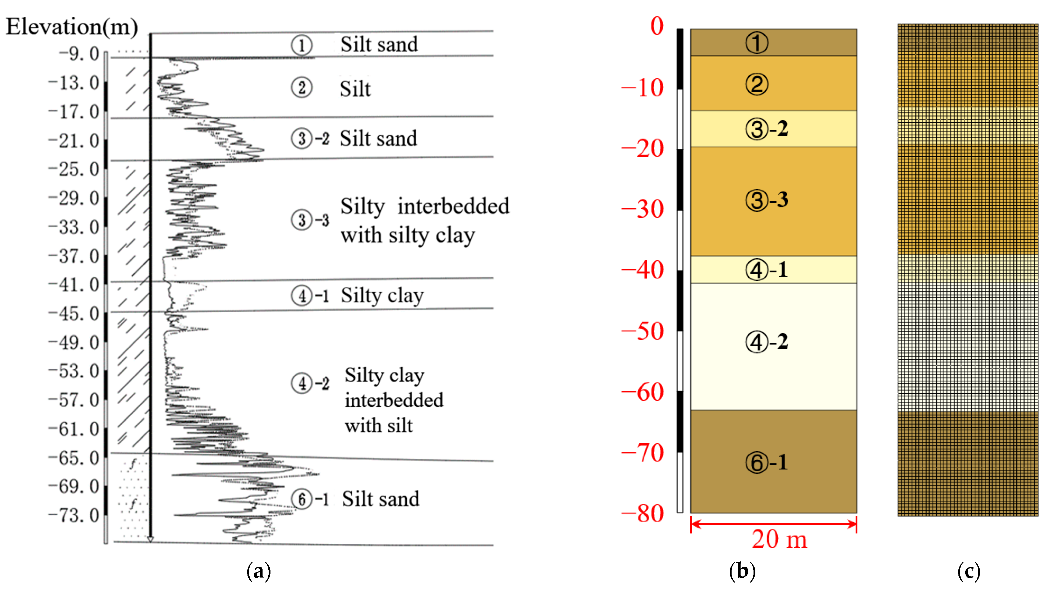
2.1. Model Generation for Saturated Seabed Foundation with Interbedded Soft Clay–Sand

According to the submarine foundation borehole data provided by the survey unit, the typical engineering geological profile of the southeast coastal area of China is shown in Figure 1a. As shown in Figure 1a, the foundation soil in the area consists of silt, silty sand, and silty clay. Compared with the silt layer, the silty sand has a greater amount of subsidence and is more easily liquefied under seismic loads.

Considering the depth of geological investigation (<80 m), the seabed foundation was simplified into a rectangular model with a 20 m width and 80 m height, as shown in Figure 1b. The model is spatially discretized using quadrilateral cells with displacement and pore pressure degrees of freedom. The cell size is about 0.5 m × 0.5 m, the total number of cells is 6400, and the total number of degrees of freedom is 19,200. The meshing of the numerical model is shown in Figure 1c.

After the following two randomized processes, 1000 sets of clay and sand interspersed seabed foundation models were established:

(1)

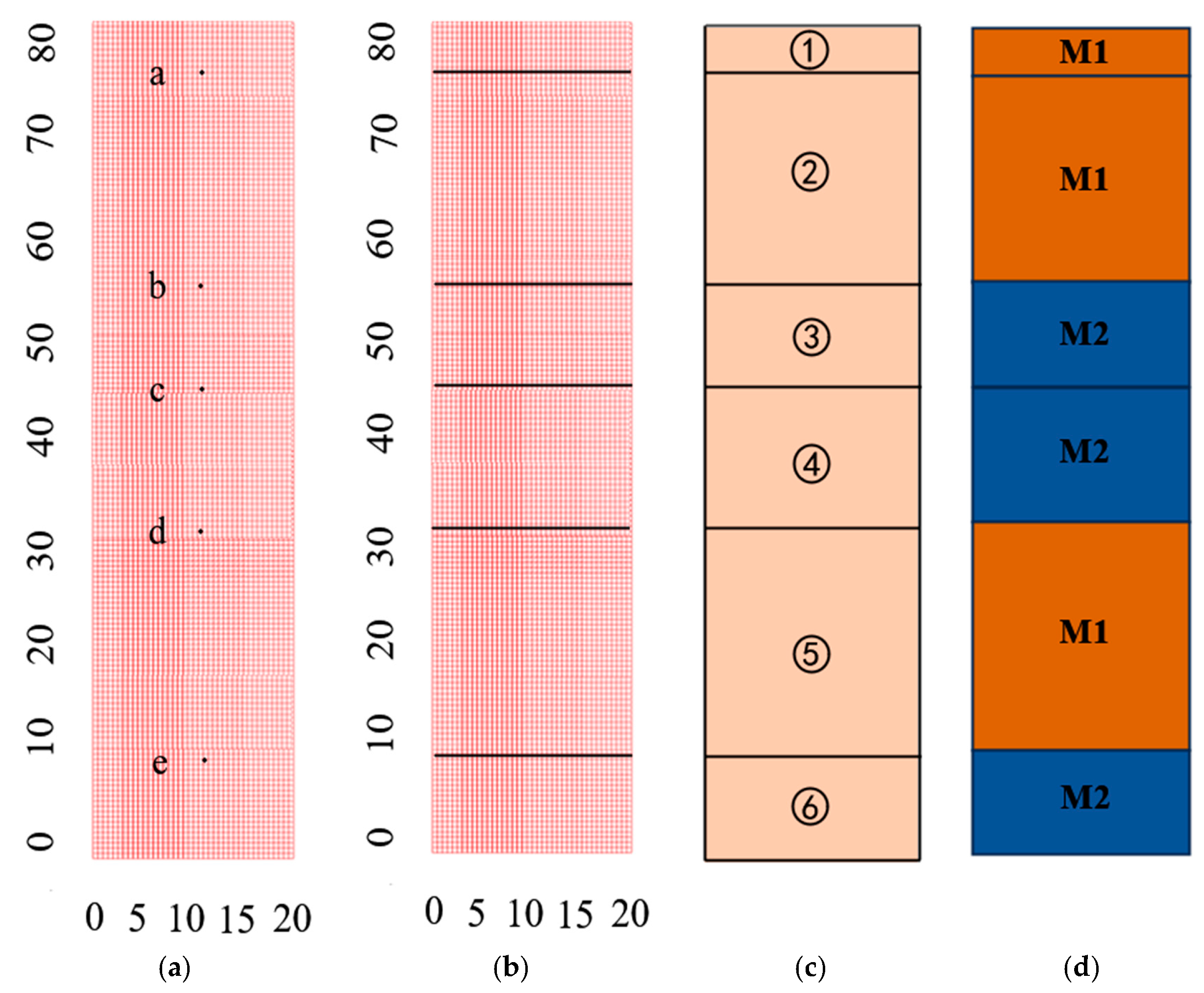
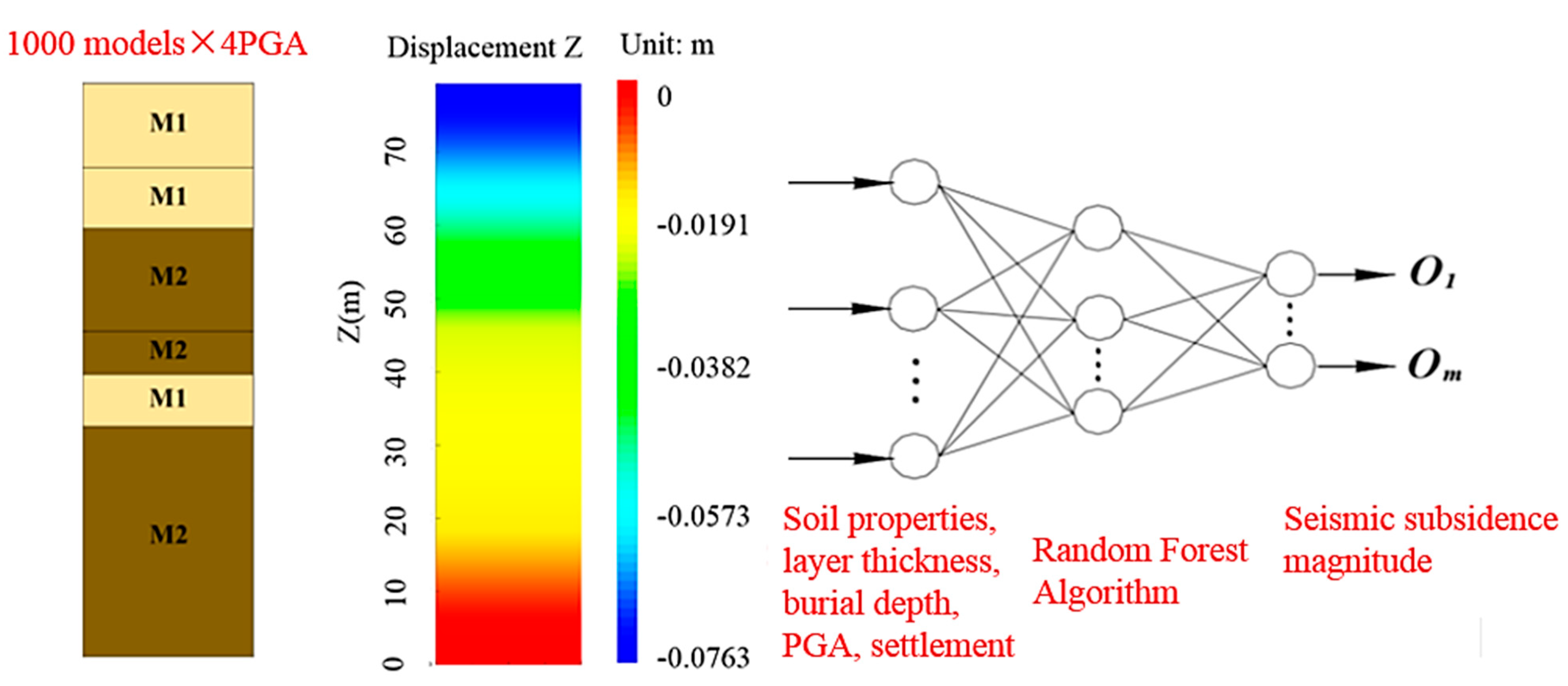
The first randomization process is to randomly generate 5 numbers, a, b, c, d, and e, in the interval range [0, 80] and simultaneously satisfy the following conditions: $0<a<b<c<d<e<80$, $2\le a\le 30, 2\le b-a\le 30$, $2\le c-b\le 30, 2\le d-c\le 30,$ and $2\le e-d\le 30, 2\le 80-e\le 30$. By this stochastic process, the seabed foundation with a thickness of 80 m can be randomly divided into 6 layers, and the thickness of each layer is between 2 m and 30 m, as shown in Figure 2a–c;

(2)

The second randomization process is to randomly select n ($1\le n\le 6$) layers of soil out of the 6 layers, whose material properties are set as clay layer (M1), and the remaining 6 n layers are set as sandy soil layers (M2). See Figure 2d.

The above-randomized algorithm was used to generate 1000 sets of seabed foundation models with interbedded clay and sand. And it can be guaranteed that the thicknesses and burial depths of the clay and sand layers were randomly distributed and that the thicknesses of the clay and sand layers ranged from 2 m to 30 m.

2.2. Constitutive Models and Validation

Numerous studies [25,26,27,28,29] have shown that pore water pressure accumulation will occur within the seabed foundation if loading continues to be applied after the sea sand soil has reached its peak strength under dynamic loading. Sand seabed foundations will soften and liquefy, thereby compromising the foundation’s load-bearing capacity. The advanced constitutive model PZIII (Pastor-Zienkiewicz III) proposed by Pastor et al. [30] based on the generalized plasticity theory is proposed to capture the mechanical behaviors of sand seabed foundations that are able to be liquefied and softened under seismic loading [31]. The reliability has been verified by Zienkiewicz et al. [32] through a series of indoor tests with monotonic and cyclic loading. Jeng et al. [33] embedded the PZIII model into FssiCAS and performed the numerical simulation of centrifuge experiments for loose sand (natural void ratio e₀ = 0.831) and dense sand (natural void ratio e₀ = 0.603). A comparison of numerical results provided by FssiCAS and Jeng’s experiment data on loose sand and dense sand is shown in Figure 3. The close agreement between numerical simulation results and the experimental measurements validates the PZIII model’s efficacy in simulating sand’s dynamic response characteristics.

Many studies [34,35,36,37,38] have shown that marine clays are subject to stiffness degradation and shear modulus folding under complex stress states. The elasto-plastic dynamic constitutive model of soft clay developed by Feng et al. [39] based on the critical state and boundary surface theoretical framework was proposed to capture the mechanical behavior of submarine foundations of clay layers. In this study, Soft Clay model was developed and embedded in the finite element software FssiCAS V3.5.0, and the reliability of the Soft Clay model was verified by the isotropic compression test, isotropic compression–unloading-reloading test, triaxial drainage compression test, and undrained dynamic triaxial test. Numerical predictions from FssiCAS were validated against experimental data reported by Fei et al. [40], which are shown in Figure 4. A high degree of concordance is observed between FssiCAS simulations and experimental results, which indicates that the Soft Clay model has a high degree of reliability in describing the static and dynamic mechanical behavior of clay.

2.3. Parameter Settings

2.3.1. Parameters of the Constitutive Models

Zhao et al. [2] carried out a series of indoor dynamic triaxial and resonant column tests on field soil samples for soft clay and sandy soils in the southeast coastal region of China. Zhao et al. obtained the mechanical parameters of soft clay and sandy soil, as shown in

Table 1. Parameters of sand and soft clay soil foundation.

Foundation Soil	Initial Void Ratio ${\mathit{e}}_0$	Permeability Coefficient/(m·${\mathbf{s}}^{-1}$)	Compression Index λ	Rebound Index κ	Failure Stress Ratio ${\mathit{M}}_{\mathit{g}}$	Cohesion/KPa	Internal Friction Angle/(°)
Sand	0.728	${3\times 10}^{-6}$	0.011	0.001	1.25	—	—
Soft clay	0.980	${1.8\times 10}^{-9}$	—	—	—	40	15

. The e–p curve of sandy soil is shown in Figure 5.

Based on the mechanical parameters of soft clay and sand provided by Zhao et al., some of the calculation parameters of the Soft Clay model and PZIII can be converted, such as the slope of the critical state (M_g), the slope of the straight line at the phase transition point (M_f), and so on. The plastic modulus parameter H₀ can be derived from the compression and expansion indices, while the bulk modulus (K₀) and shear modulus (G₀) can be derived from the e–p curve. Combined with the experimental data provided by the survey and design unit, the calculation parameters for Soft Clay model and PZIII can be determined, as shown in

Table 2. Parameters of the PZIII model.

K0/(Pa)	G0/(Pa)	Mg	αg	Mf	αf	β0	β1	H0	Hu0/(Pa)	γDM	γu	${\mathit{p}}_0^{\mathbf{\prime }}$
2.092 × 106	1 × 108	1.25	0.45	0.95	0.45	4.2	0.2	442.14	442.1 × 103	1	1	1 × 103

and

Table 3. Parameters of the Soft Clay model.

Normal Consolidation Line Slope λ	Rebound Modulus κ	Poisson’s Ratio ν	Critical State Stress Ratio M	Normal Consolidation Line Intercept N	Critical State Line Intercept Γ	Boundary Surface Model Parameters n
0.14	0.043	0.38	1.25	1.13	1.00	1.60

.

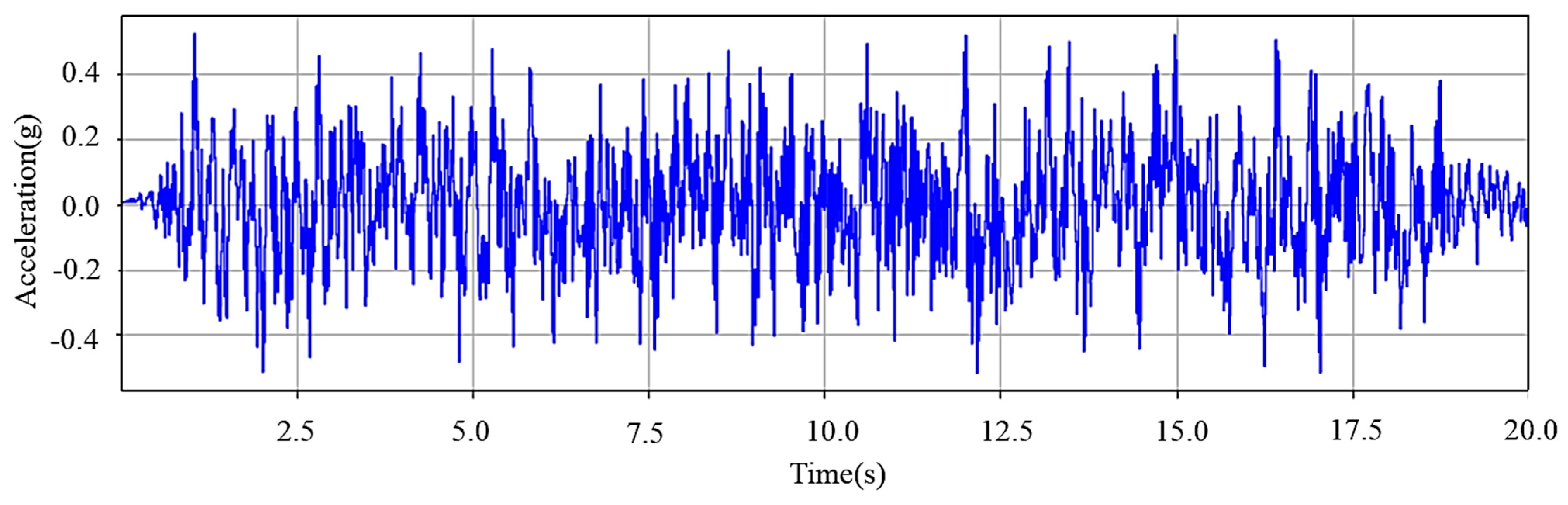
2.3.2. Seismic Wave Parameters

According to the seismic design code, the site is classified as Type II, and the fortification intensity is VII–VIII. According to the field data provided by the investigation and design unit, the characteristic period of the site is about 0.35 s, and the horizontal influence coefficient is 0.45. Parameters characterizing the seismic response spectrum were established, as detailed in

Table 4. Response spectrum parameters of seismic wave.

Site Category	Design Intensity	Peak Ground Acceleration (PGA) (g)	Characteristic Period (s)	Horizontal Influence Coefficient
II	VII–VIII	0.05, 0.1, 0.2, 0.4	0.35	0.45

. The corresponding artificial seismic waves can be generated according to the parameters of the seismic response spectrum, as shown in Figure 6 (PGA = 0.05 g). Four artificial seismic waves can be obtained by scaling the amplitudes of the seismic waves with PGAs of 0.05 g, 0.1 g, 0.2 g, and 0.4 g, respectively. The four types of seismic waves were applied to the bottom of 1000 models of seabed foundations with interbedded soft soil–sand for 4000 sets of case studies.

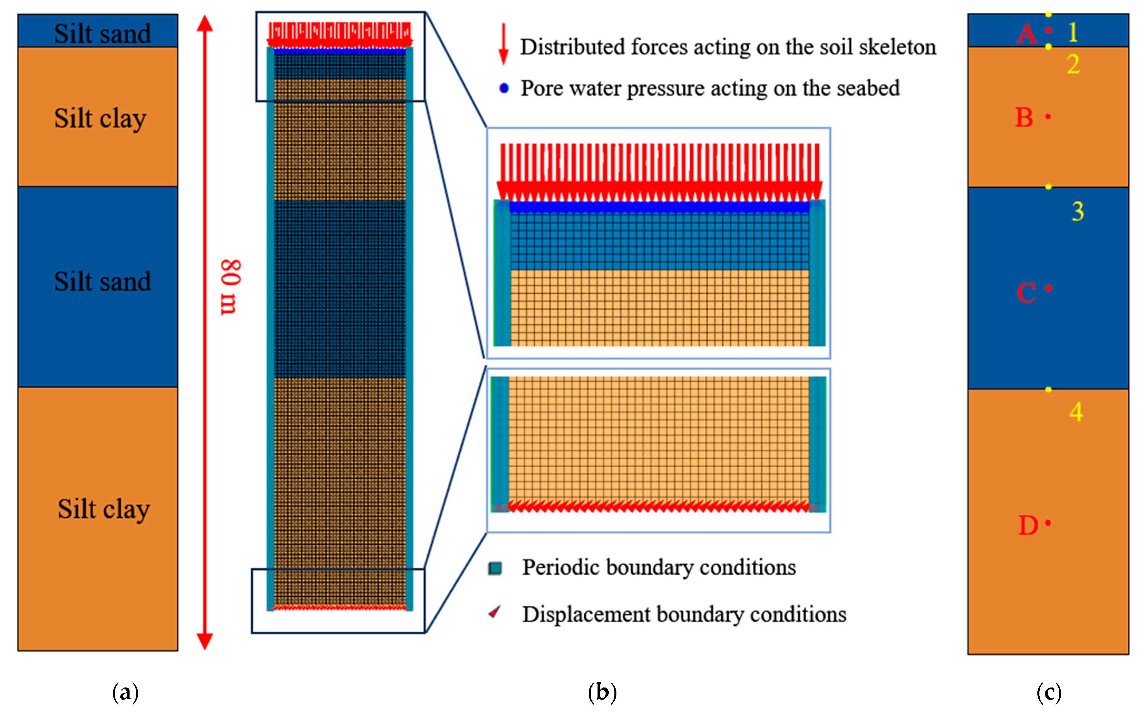
2.4. Boundary Conditions and Monitoring Points

Model 1 is selected as a typical model for result analysis and discussion. Model 1 consists of four layers, and the soil types of each layer from the bottom of the model upwards are silt clay, silt sand, silt clay, and silt sand. The thicknesses of each layer are 33 m, 25.5 m, 17.5 m, and 4 m, respectively, as shown in Figure 7a.

The boundary conditions implemented for Model 1 are shown in Figure 7b. The xz-directional displacements are fixed at the bottom of the model and the excited seismic wave is input at the bottom; the periodic boundaries are implemented laterally to minimize seismic wave reflection along the model edges; and a hydrodynamic boundary is applied at the top of the model, which includes the boundary condition of the distributed force acting on the soil skeleton and the boundary condition of the pore pressure acting on the pore fluid. Some monitoring points were selected within the model to assist in the analysis of the results, and the locations of the monitoring points are shown in Figure 7c. Monitoring points 1~4 are used to monitor the displacement and acceleration response of the seabed soil surface, and monitoring points A~D are arranged to capture the pore pressure dynamics and effective stress evolution in the seabed foundation. The coordinates of each monitoring point are A (10, 0, 78), B (10, 0, 67.25), C (10, 0, 45.75), D (10, 0, 16.5), 1 (10, 0, 80), 2 (10, 0, 76), 3 (10, 0, 58.5), and 4 (10, 0, 33), respectively.

3. Analysis and Discussion of Results

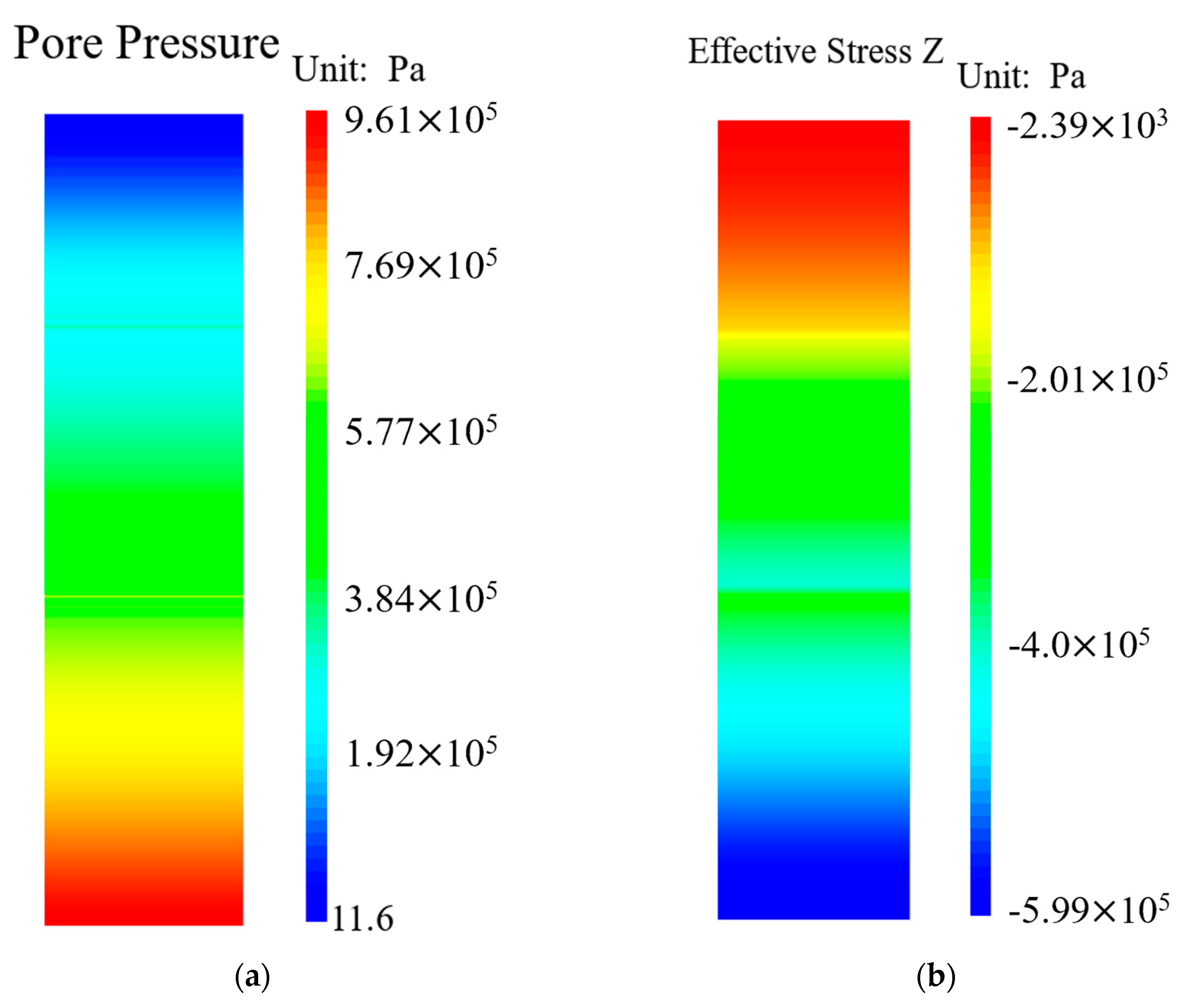
3.1. Initial State

The initial stress field of the seabed is obtained, preceding the dynamic response simulations. Figure 8 shows the steady state of the seabed soil after the consolidation is finished under gravity and hydrostatic pressure. The displacements occurring at the seabed foundation are distributed in an overall downward laminar pattern along the z-direction, with the largest vertical displacements occurring at the surface of the formation. Both the pore pressure and effective stress magnitudes are directly proportional to the soil layer depth.

3.2. Seismic Dynamic Response Characteristics

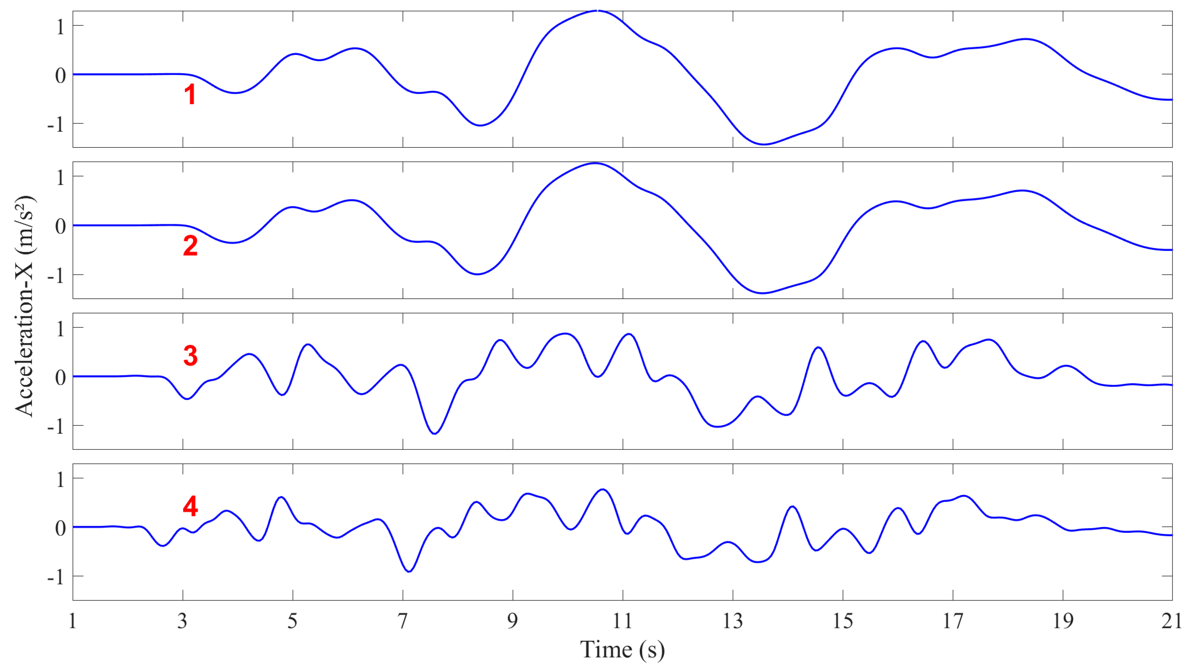
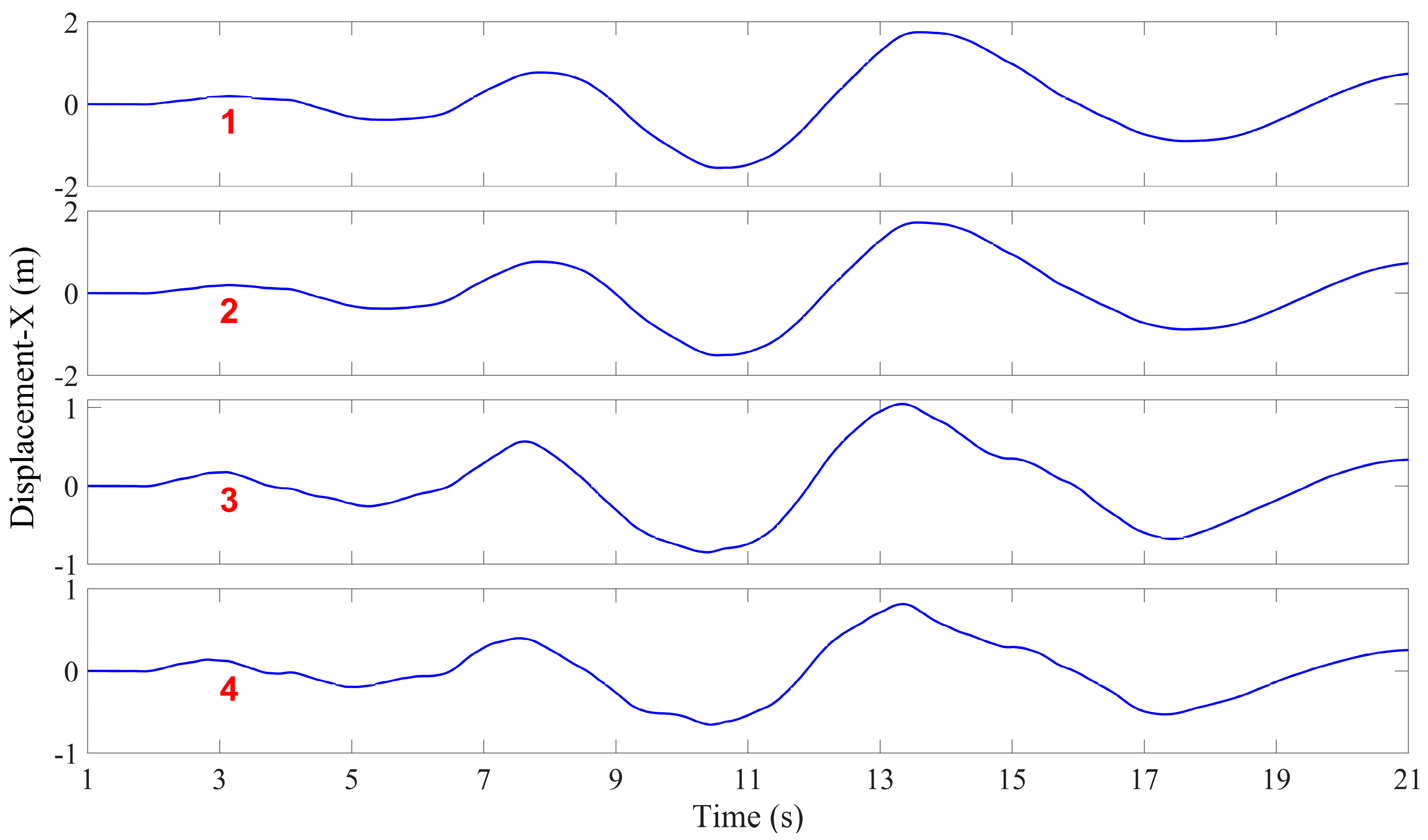
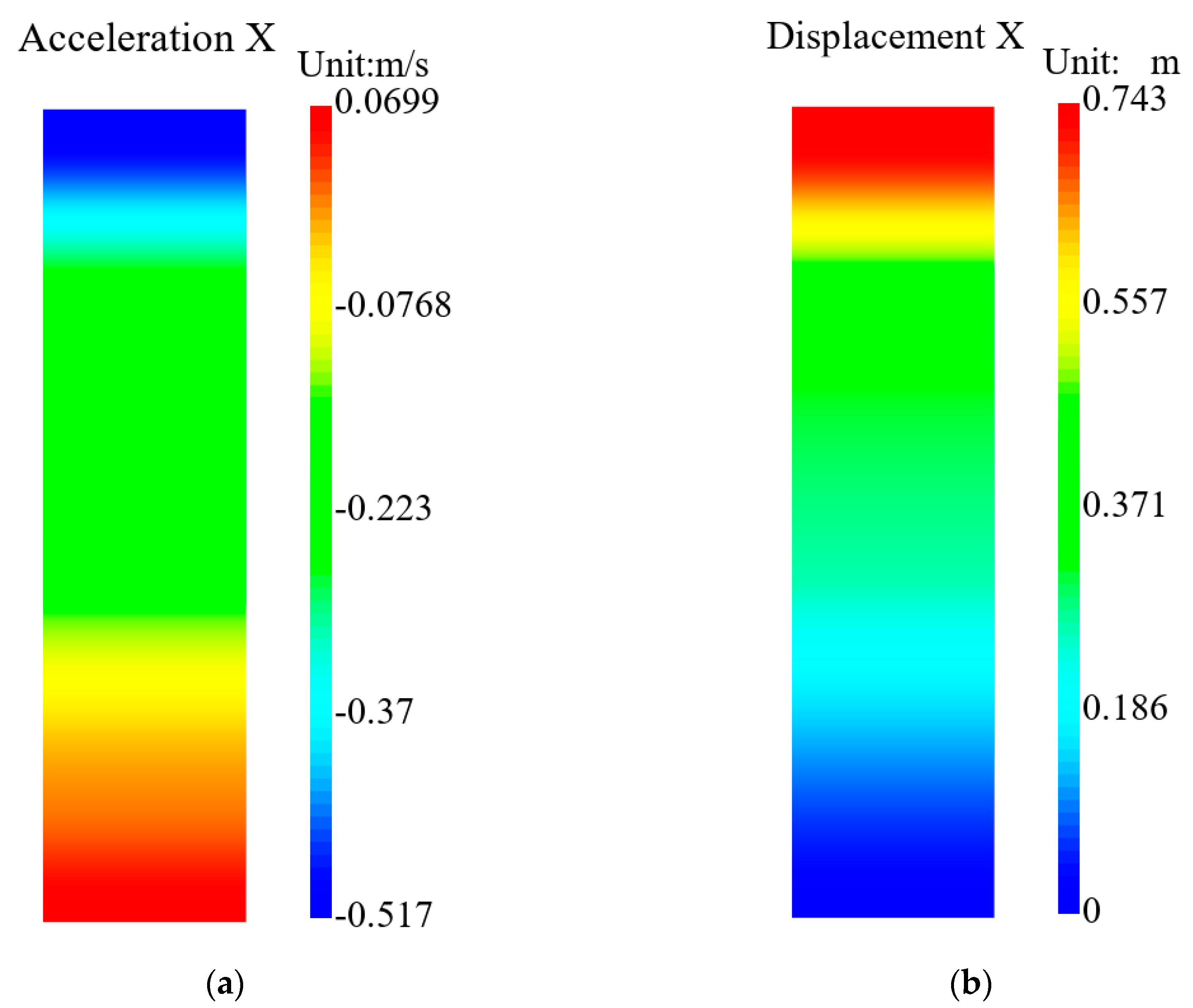
3.2.1. Acceleration and Displacement Response

The dynamic response of the foundation with interbedded clay–sand is subsequently examined. The acceleration curves at monitoring points 1, 2, 3, and 4 are shown in Figure 9. It can be seen that (1) the acceleration spikes show a certain degree of amplification when the seismic wave propagates upward from the bottom of the model; and (2) the high-frequency components of the seismic wave propagated in the seabed soil are absorbed and the energy is significantly attenuated. When the seismic waves propagate in a pore medium, a series of complex physical processes will occur, attenuating the energy and the absorption of the high-frequency components. Seismic wave propagation induces vibrations in the solid skeleton and also causes the relative motion of the fluid in the pore space. This solid–fluid interaction is an important mechanism for energy attenuation. From a microscopic point of view, viscous friction occurs at the interface between the solid particles and the fluid as the wave propagates. This friction converts the mechanical energy of the seismic wave into thermal energy, resulting in energy loss. For high-frequency components, the relative motion between the solid skeleton and the fluid in the pore medium is more violent due to its short vibration period. High-frequency waves propagating in pore media experience more solid–fluid interaction interfaces per unit of time, and therefore, the rate of energy loss is faster. The x-directional acceleration distribution of the seabed foundation at the typical moment (t = 21 s) is shown in Figure 11a. This figure reveals the amplification of seismic wave peaks with increasing height very clearly.

The x-directional displacement response of the typical positions in the soil foundation under the seismic wave action is shown in Figure 10. Under the amplification effect of seismic waves, the x-direction displacement amplitude of the soil body increases with decreasing burial depth of the soil layer. The displacement response period is long due to the attenuation of seismic wave energy and the absorption of high-frequency components. There is no obvious cumulative displacement of the seabed foundation, and the x-direction displacement of the seabed soil body is about 0.5 m at the end of the seismic action. The x-direction displacement of the seabed foundation at the end of the seismic action (t = 21 s) is shown in Figure 11b. Horizontal displacements of the seabed foundation show a uniform laminar distribution under the constraints of the periodic boundary conditions.

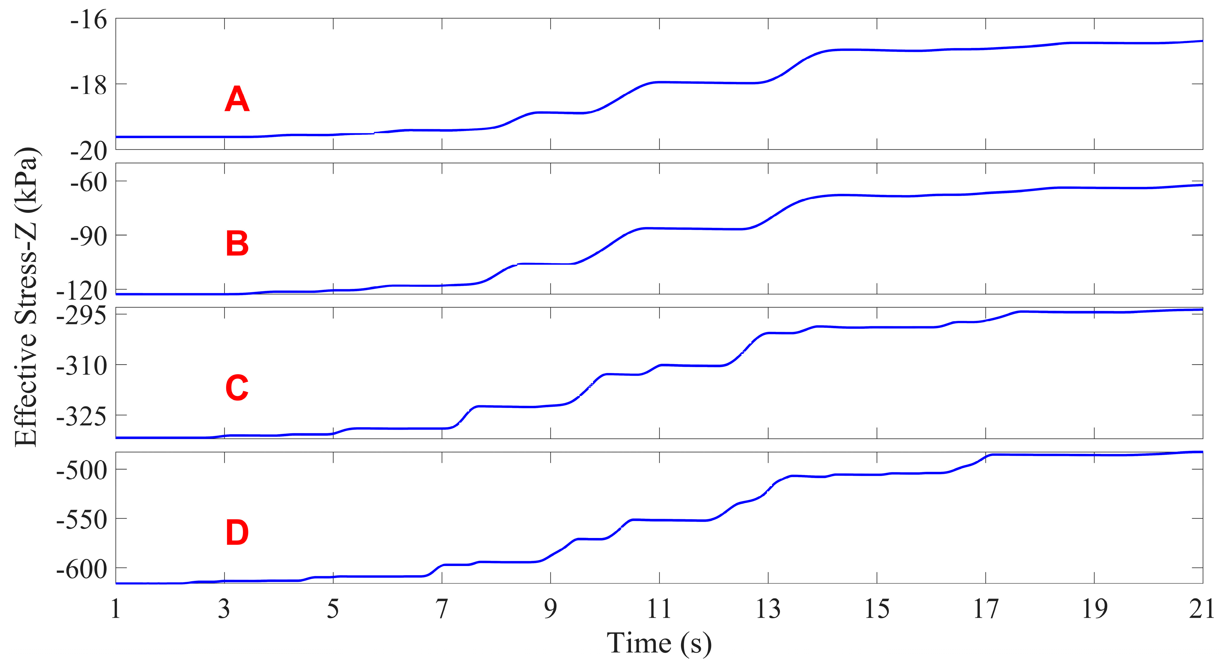
3.2.2. Pore Pressure and Effective Stress Response

The seismic-induced pore pressure responses recorded at positions A to D are presented in Figure 12. The initial pore pressure magnitude is proportional to the buried depth of the soil layer. During the period of seismic wave action (1–21 s), the pore water in the soil cannot be discharged effectively, and the pore pressure accumulates and rises. With increasing depth, excess pore pressures demonstrate amplified magnitudes, peaking at approximately 120 kPa at monitoring point D. The pore pressure distribution at the typical time (t = 21 s) is shown in Figure 14a. The pore pressures in the soil foundation are distributed in a distinct laminar pattern, influenced by the distribution of the soil layers.

The z-direction effective stresses at the four monitoring points (A, B, C, and D) are shown in Figure 13. Within the 1–21 s seismic phase, the seabed effective stress exhibits monotonic reduction characteristics (the compressive stress is negative). The greater the burial depth of the soil layer, the greater the decrease in effective stress. It is certain that some degree of softening occurred in the seabed foundation. Since the model is a free-field seabed foundation with no structures present, the total stress can be assumed to be essentially constant for a point in the seabed soil. Then, the effective stress exhibits a monotonic reduction concomitant with pore pressure accumulation in the effective stress theory. The response patterns of pore pressure and effective stress shown in Figure 12 and Figure 13 coincide with this principle. The distribution of effective stresses in the seabed soil at the end of the seismic force is shown in Figure 14b, and the effective stress in the z-direction of the soil shows a clear stratified distribution.

3.2.3. Assessment of Liquefaction Zones

Under seismically induced cyclic loading, the accumulation of pore water pressure in seabed foundations induces effective stress degradation, leading to soil softening and even potential liquefaction. It can be concluded from the presence of pore pressure and the effect of the force response that some degree of softness occurs in the seabed foundation. The next step is to further determine whether liquefaction occurred in the seabed foundation. In this study, a judgment criterion based on pore pressure is used to evaluate the distribution of liquefaction zones; liquefaction of the seabed is considered to occur when the excess pore pressure approaches or exceeds the initial effective stress. This liquefaction judgment criterion can be expressed as follows:

$$L_p={\displaystyle \frac{∆P_{\mathrm{w}}}{{\sigma }_z^{\prime }}}$$

where $L_p$ is the liquefaction potential, which may also be referred to as the pore pressure ratio, $∆P_{\mathrm{w}}$ is the excess pore water pressure in the seabed soil, which is the pore water pressure exceeding the hydrostatic pressure, and ${\sigma }_z^{\prime }$ is the initial effective stress along the z-direction.

When the pore pressure ratio ($Lp$) approaches 1.0, it indicates soil liquefaction. The distribution of the liquefaction potential $Lp$ of the seabed foundation at the end of seismic wave action is shown in Figure 15. From the figure, it can be seen that the distribution of the liquefaction potential is closely related to the stratification and materials of the seabed; compared with the sand layer, the liquefaction potential of the clay layer of the seabed foundation is larger; the maximum pore pressure ratio is about 0.62; and the seabed foundation is softened to a certain extent under seismic excitation without liquefaction.

3.3. Post-Earthquake Consolidation

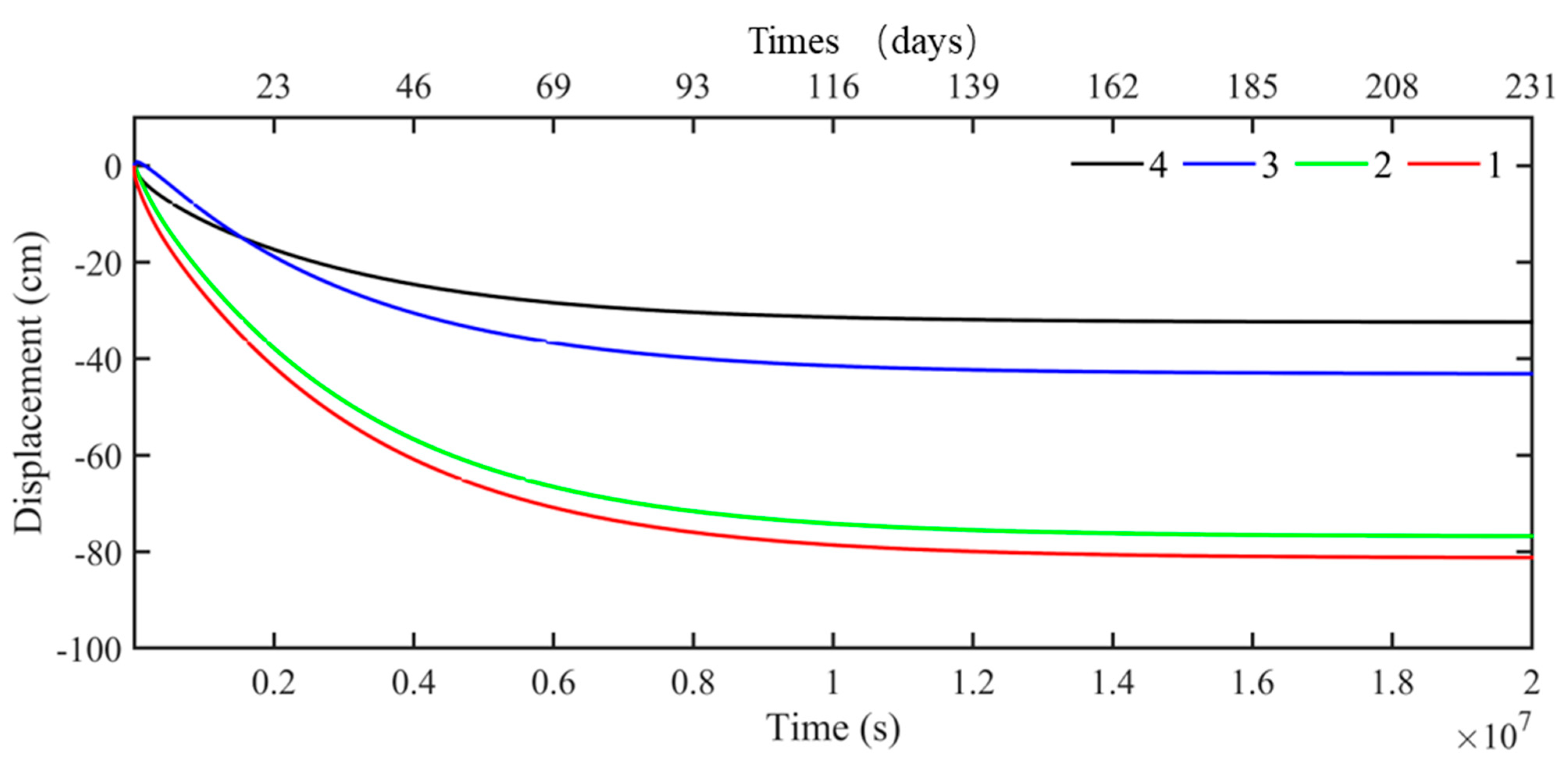
Compared with seismic action, post-seismic consolidation is a long process, often lasting months or even years. During the post-seismic consolidation phase, further settlement of the seabed foundation will occur along with the dissipation of the excess pore pressure.

3.3.1. Displacement

The time history of z-directional displacement response at the typical positions during the post-seismic consolidation process is shown in Figure 16. The horizontal axis at the top of the diagram is scaled in days, while the bottom axis uses seconds. It can be seen that, during the post-seismic consolidation phase, significant vertical settlement occurred in the seabed foundations; the amount of settlement decreased gradually with the depth of the soil layer; and the maximum settlement occurred on the surface of the seabed foundation soil, which was about 0.82 m.

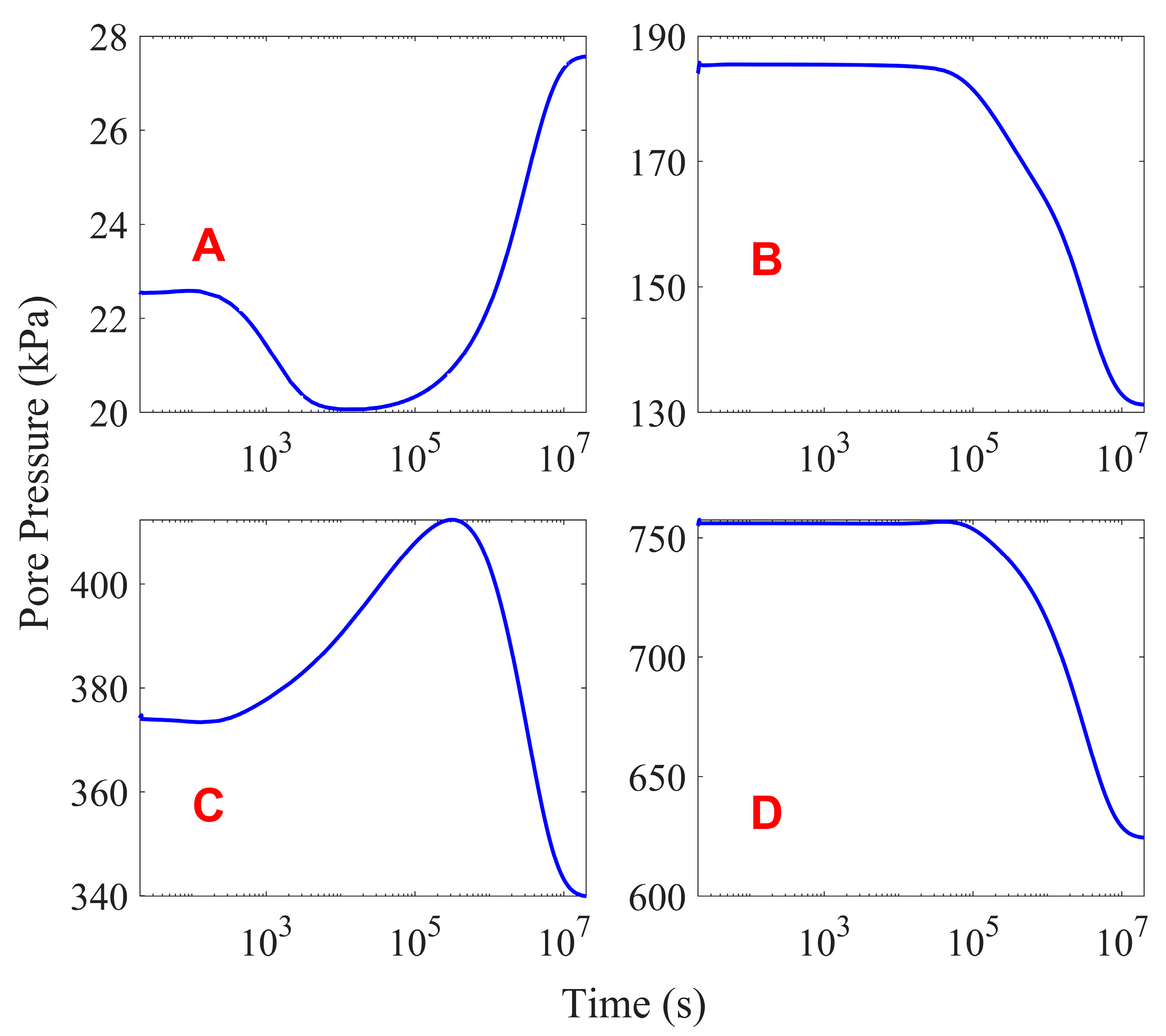
3.3.2. Pore Pressure

The variations in pore pressure at monitoring locations A–D throughout the post-seismic consolidation phase are illustrated in Figure 17. A, B, C, and D are located within four soil layers from top to bottom, where B and D are located in the clay layer and A and C are in the sand layer. Figure 17 shows that the pore water pressure continues to decrease at locations B and D until the excess pore pressure completely dissipates. For point A, the pore pressure first decreased and then increased significantly. At the end of consolidation, the pore pressure at point A increased by about 5 kPa compared with the initial value, which is an interesting phenomenon. It is known from the previous analyses that the shallow layer of the seabed subsided significantly during the post-earthquake consolidation stage, and the seabed surface subsided by about 0.8 m. Point A was located 2 m below the seabed surface, and the final settlement at point A at the end of the post-earthquake consolidation was about 0.6 m. Disregarding the change in the static water level, the depth of water at point A increased by 0.6 m after the post-earthquake consolidation. It can be concluded from these results that the increase in pore pressure at point A is due to the increase in hydrostatic pressure at this position.

3.4. Statistics of 4000 Case Results

The seismic dynamic response characteristics of a typical case have been analyzed in detail. Next, the results of the 4000 cases are analyzed statistically. Figure 18 shows the relationship between seabed settlement and the average burial depth of the clay layer, the relationship between seabed settlement and the percentage of clay layer thickness, and the relationship between the percentage of the foundation settlement of the clay layer and the percentage of clay layer thickness. The average burial depth of the clay layer is defined as follows:

$$d=\sum d_i*{\displaystyle \frac{t_i}{T}}$$

where $d$ is the average buried depth of the clay layer, $d_i$ is the buried depth of the clay layer $i$, $t_i$ is the thickness of the clay layer $i$, and $T$ is the total thickness of the clay layer.

It can be found that the larger the PGA, the larger the seabed foundation settlement; the shallower the average depth of the clay layer, the larger the seabed foundation settlement; and the larger the percentage of the clay layer thickness, the larger the seabed foundation settlement. The statistics of the 4000 sets of data show obvious regularities, which indicates that the data quality can be guaranteed, laying a solid foundation for the training and validation of the rapid prediction model.

4. Rapid Prediction Model Based on Machine Learning Theory

4.1. Rapid Prediction Model for Seismic-Induced Subsidence of Seabed Foundation with Interbedded Soft Clay–Sand

In this paper, 4000 sets of case simulations were carried out using the finite element computational platform FssiCAS to investigate the characteristics of the seismic dynamic response of free-field seabed foundations under different geological stratigraphic conditions and different seismic wave PGAs, respectively. The model characteristics of each calculation case are extracted: the number of layers of the seabed foundation, the thickness and burial depth of the layers, the material properties of the layers, the seismic wave PGA, and the characteristics of the dynamic response of the seabed foundation under the seismic action: the final settlement of the seabed foundation, the liquefaction potential, and the liquefaction depth. A database is obtained after processing the above data. The development of fast prediction models requires two steps: data training and reliability verification [41]. Therefore, the 4000-sample dataset underwent partitioning into training and testing subsets, in which 3200 sets of numerical simulation results were used for model training, and 800 sets were used for validating the model’s reliability.

There are many algorithms that have been used to develop machine learning models such as the Random Forest algorithm, Gradient Ascent algorithm, XGBoost algorithm, and Linear Regression algorithm. Studies have shown that the Random Forest algorithm has good applicability and reliability in the foundation settlement prediction problem [42,43,44,45,46,47]. In this study, the Random Forest algorithm is selected to establish the prediction model. The establishment of the rapid prediction model for the seismic-induced subsidence of seabed foundations with interbedded soft clay–sand is illustrated in Figure 19.

4.2. Model Reliability Verification

The test set is used to validate the reliability of the rapid prediction model for the seismic settlement of seabed foundations with interbedded clay–sand, and a quantitative evaluation of its reliability is provided. R², a widely utilized metric in regression analyses, was employed to evaluate the predictive accuracy of the settlement, liquefaction potential (L_potential), and liquefaction depth (L_depth) models, with values approaching one signifying enhanced predictive consistency. R² is defined as follows:

$$R^2=1- {\displaystyle \frac{\sum _i{(y_i-{\hat{y}}_i)}^2/n}{\sum _i{(y_i-\hat{y})}^2/n}}$$

The prediction performance of the Random Forest model (RFM) is illustrated in Figure 20. As observed from the figure, the scatter points determined by the numerical simulation results and the prediction results provided by the rapid prediction model are uniformly distributed around the diagonal line (with a slope of one), which indicates that there is a highly linear relationship between the prediction results and the numerical simulation results. The rapid prediction model for the seismic-induced subsidence of seabed foundations with interbedded soft clay–sand, as developed in this study, shows commendable accuracy in the prediction of the settlement, liquefaction potential (L_potential), and liquefaction depth (L_depth), with an R² value exceeding 0.86.

A histogram of prediction errors for the settlement, liquefaction potential (L_potential), and liquefaction depth (L_depth) is shown in Figure 21. The percentage error between the simulated and predicted values is plotted on the horizontal axis, with the frequency displayed on the vertical axis. It can be found that the prediction errors are primarily distributed within the range of ±0.6%. These results indicate that the Random Forest-based machine learning model can effectively predict the seismic settlement characteristics of foundations with interbedded soft clay–sand and its predictions have a high level of reliability.

5. Conclusions

The seismic dynamic response characteristics of saturated seabed foundations with interbedded soft clay–sand were systematically investigated, with a focus on revealing their subsidence behavior. This study employed the boundary-surface-theory-based Soft Clay model to simulate the mechanical behavior of saturated soft clay, complemented by the generalized elastoplastic constitutive model PZIII for sand. Leveraging the finite element analysis platform FssiCAS, a comprehensive set of 4000 numerical simulations were conducted to analyze the seismic dynamic responses, providing robust insights into the behavior of such complex seabed foundations under seismic conditions. Based on the numerical simulation results of these 4000 cases, a rapid prediction model for the seismic settlement of seabed foundations with interbedded soft clay–sand is developed. The principal findings of this investigation can be summarized as follows:

(1)

A comparative analysis of the experimental and numerical simulation results confirmed that the Soft Clay and PZIII constitutive models integrated in FssiCAS effectively characterize the mechanical response of clay–sand composite soil foundations;

(2)

Under the sustained action of seismic loading, the pore water pressure within the saturated seabed foundations with interbedded soft clay–sand accumulates, while the effective stress decreases, leading to significant seabed softening. During the post-seismic consolidation phase, the settlement of the seabed foundation soil is pronounced, with settlements up to 0.8 m;

(3)

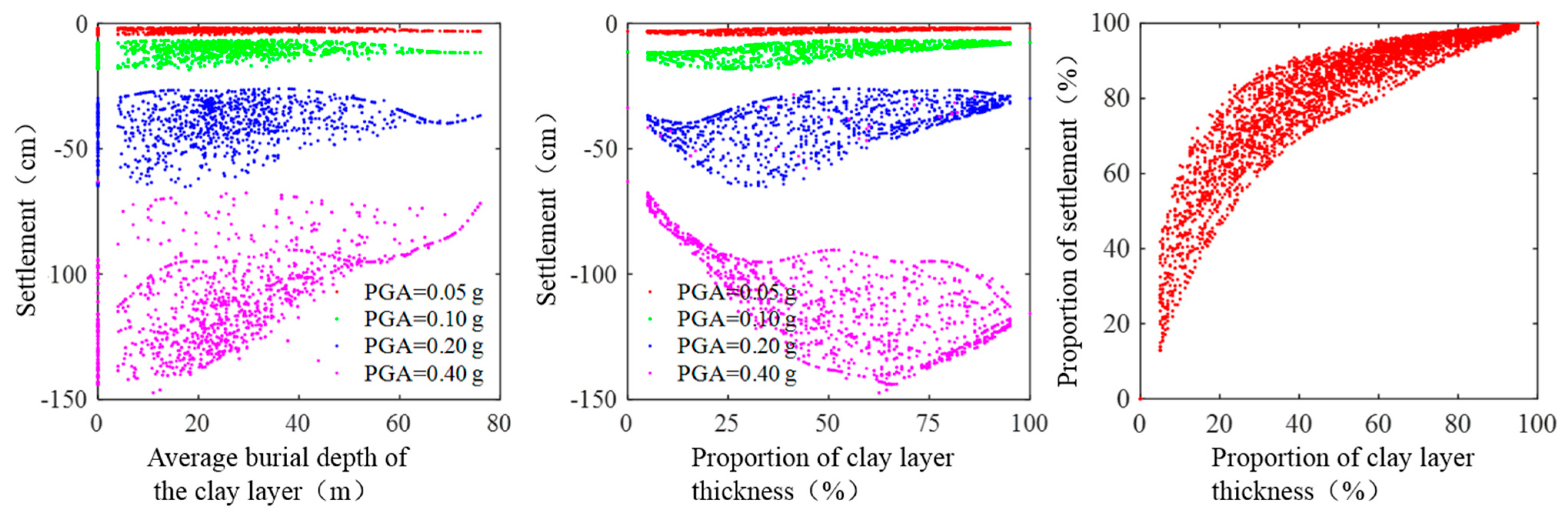
The settlement of the saturated seabed foundations with interbedded soft clay–sand under seismic loading is significantly affected by the PGA, clay layer thickness, and burial depth. The greater the PGA, the larger the seabed settlement; the shallower the burial depth of the clay layer, the greater the seabed settlement; and the higher the proportion of clay layer thickness, the greater the seabed settlement;

(4)

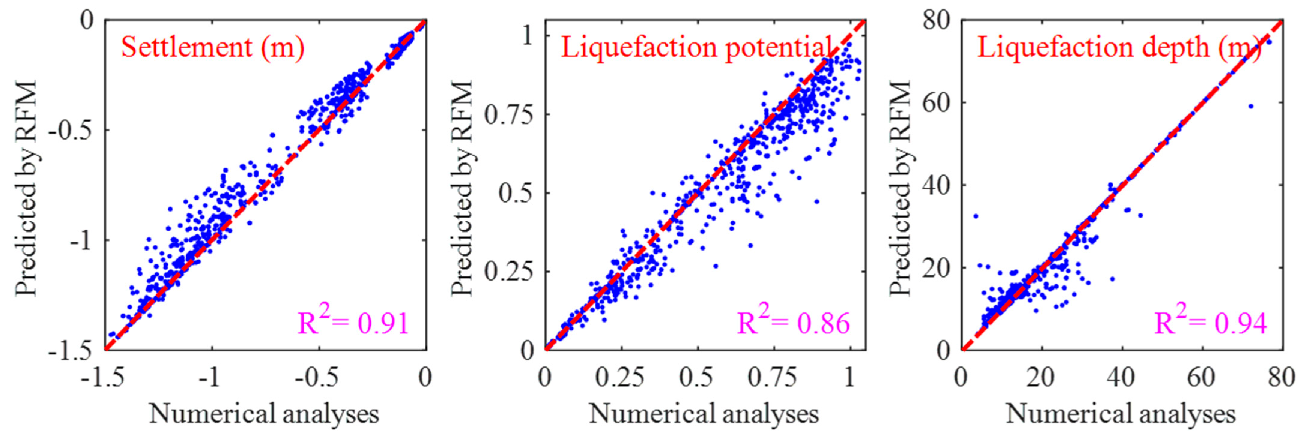
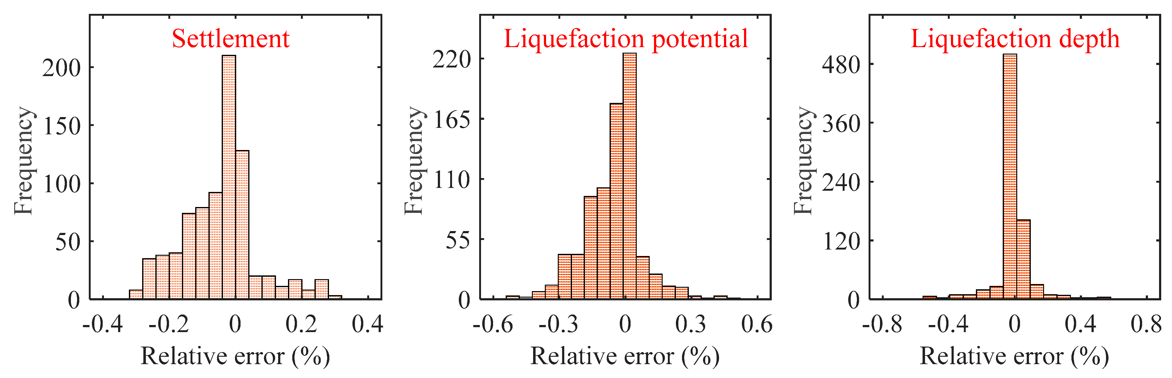
The Random Forest-based machine learning model can rapidly predict the seismic-induced settlement behavior of submarine foundations in soft clay–sand interlayers with a prediction accuracy of R² = 0.91, which verifies its high reliability. This study provides a new technical path for the rapid prediction of the seismic settlement of submarine foundations in engineering. It also shows that physically constrained large-scale artificial intelligence models have broad application prospects in the field of engineering design, assessment, and prediction.

References

1. Liu, Y.-X.; Guo, Y.; Huang, C. Comparative Study on the Development Situation and Policies of Offshore Wind Power in China and Abroad. Res. Sci. Technol. Manag. 2023, 43, 65–70. (In Chinese) [Google Scholar]
2. Zhao, L.-Y.; Shan, Z.-G.; Wang, M.-Y. Analysis of Horizontal Ground Liquefaction Characteristics of South Yellow Sea Offshore Wind Farm under Earthquake Action. Geotech. Eng. Soil Mech. 2022, 43, 13. (In Chinese) [Google Scholar]
3. Zhang, Z.; Li, Y.; Xu, C.; Du, X.; Dou, P.; Yan, G. Study on seismic failure mechanism of shallow buried underground frame structures based on dynamic centrifuge tests. Soil Dyn. Earthq. Eng. 2021, 150, 106938. [Google Scholar] [CrossRef]
4. Zhou, Y.G.; Liu, K.; Sun, Z.B.; Chen, Y.M. Liquefaction mitigation mechanisms of stone column-improved ground by dynamic centrifuge model tests. Soil Dyn. Earthq. Eng. 2021, 150, 106946. [Google Scholar] [CrossRef]
5. Li, L.-Y.; Rajesh, S.; Chen, J.-F. Centrifuge model tests on the deformation behavior of geosynthetic-encased stone column supported embankment under undrained condition. Geotext. Geomembr. 2021, 49, 550–563. [Google Scholar] [CrossRef]
6. Maharjan, M.; Takahashi, A. Centrifuge model tests on liquefaction-induced settlement and pore water migration in non-homogeneous soil deposits. Soil Dyn. Earthq. Eng. 2013, 55, 161–169. [Google Scholar] [CrossRef]
7. Higo, Y.; Lee, C.W.; Doi, T.; Kinugawa, T.; Kimura, M.; Kimoto, S.; Oka, F. Study of dynamic stability of unsaturated embankments with different water contents by centrifugal model tests. Soils Found. 2015, 55, 112–126. [Google Scholar] [CrossRef]
8. Chakrabortty, P.; Popescu, R. Numerical simulation of centrifuge tests on homogeneous and heterogeneous soil models. Comput. Geotech. 2012, 41, 95–105. [Google Scholar] [CrossRef]
9. Yu, H.-Y.; He, G.-N.; Yang, B. Experimental Study on the Seismic Settlement Characteristics of Soft Soils. J. Dalian Univ. 1996, 76–82. (In Chinese) [Google Scholar]
10. Xie, W.; Zhang, Q.; Gao, B.; Ye, G.; Zhu, W.; Yang, Y. Shaking table tests for seismic response of jack-up platform with pile leg-mat foundation on sandy seabed. Ocean Eng. 2024, 309, 118564. [Google Scholar] [CrossRef]
11. Tsaparli, V.; Kontoe, S.; Taborda, D.M.; Potts, D.M. Vertical ground motion and its effects on liquefaction resistance of fully saturated sand deposits. Proc. R. Soc. A Math. Phys. Eng. Sci. 2016, 472, 20160434. [Google Scholar] [CrossRef]
12. Gu, L.; Zhang, F.; Bao, X.; Shi, Z.; Ye, G.; Ling, X. Seismic behavior of breakwaters on complex ground by numerical tests: Liquefaction and post liquefaction ground settlements. Earthq. Eng. Eng. Vib. 2018, 17, 325–342. [Google Scholar] [CrossRef]
13. Gu, J.-R.; Li, P.; Tian, Z.-Y.; Zhou, C.-Z.; Zhang, Y. Study on the Influence of Earthquake Motion on the Seismic Settlement of Soft Soils Based on OpenSees. J. Earthq. Eng. 2019, 41, 1339–1346. (In Chinese) [Google Scholar]
14. Gao, G.; Wang, X.; Zhu, T.; Liao, Y.; Tong, J. HSS Modeling and Stability Analysis of Single-Phase PFC Converters. In Proceedings of the 2022 IEEE Applied Power Electronics Conference and Exposition (APEC), Houston, TX, USA, 20–24 March 2022. [Google Scholar]
15. Gao, B.; Ye, G.; Zhang, Q.; Xie, Y.; Yan, B. Numerical simulation of suction bucket foundation response located in liquefiable sand under earthquakes. Ocean Eng. 2021, 235, 109394. [Google Scholar] [CrossRef]
16. Chen, W.; Huang, L.; Xu, L.; Zhao, K.; Wang, Z.; Jeng, D. Numerical study on the frequency response of offshore monopile foundation to seismic excitation. Comput. Geotech. 2021, 138, 104342. [Google Scholar] [CrossRef]
17. Ye, J.; Jeng, D.; Wang, R.; Zhu, C. A 3-D semi-coupled numerical model for fluid–structures–seabed-interaction (FSSI-CAS 3D): Model and verification. J. Fluids Struct. 2013, 40, 148–162. [Google Scholar] [CrossRef]
18. He, K.; Huang, T.; Ye, J. Stability analysis of a composite breakwater at Yantai port, China: An application of FSSI-CAS-2D. Ocean. Eng. 2018, 168, 95–107. [Google Scholar] [CrossRef]
19. Jianhong, Y.; Dongsheng, J.; Liu, P.L.; Chan, A.H.; Ren, W.; Changqi, Z. Breaking wave-induced response of composite breakwater and liquefaction in seabed foundation. Coast. Eng. 2014, 85, 72–86. [Google Scholar] [CrossRef]
20. Ye, J.; He, K. Dynamics of a pipeline buried in loosely deposited seabed to nonlinear wave & current. Ocean Eng. 2021, 232, 109127. [Google Scholar]
21. Zhao, H.-B. Predictgaoion of Settlement in Soft Soil Subgrades of Highways. J. Undergr. Space Eng. 2005, 190–192. (In Chinese) [Google Scholar]
22. Chen, X.-F.; Liu, L. Study on the Prediction Method of Settlement for Metro Tunnels Adjacent to Large Deep Excavations. Mod. Tunneling Technol. 2014, 51, 94–100. [Google Scholar]
23. Ling, X.; Kong, X.; Tang, L.; Zhao, Y.; Tang, W.; Zhang, Y. Predicting earth pressure balance (EPB) shield tunneling-induced ground settlement in compound strata using random forest. Transp. Geotech. 2022, 35, 100771. (In Chinese) [Google Scholar] [CrossRef]
24. Wang, X.; Chen, F.-D.; Liu, K.; Wu, X.-G.; Chen, B. Study on Building Settlement Induced by Tunnel Shielding Based on Random Forest—Support Vector Machine. J. Civ. Eng. Manag. 2021, 38, 86–92. (In Chinese) [Google Scholar]
25. Seed, H.B.; Booker, J.R. Stabilization of Potentially Liquefiable Sand Deposits Using Gravel Drain Systems; Earthquake Engineering Research Center, University of California El Cerrito: Berkeley, CA, USA, 1976. [Google Scholar]
26. Zhang, T. Deformation Characteristics and Micromechanical Fracture Rules of Sand Soil under High Stress Conditions and Triaxial Compression and Shear Deformation. Ph.D. Thesis, China University of Mining and Technology, Xuzhou, China, 2021. (In Chinese). [Google Scholar]
27. Zhang, J.-M.; Wang, R. Large post-liquefaction deformation of sand: Mechanisms and modeling considering water absorption in shearing and seismic wave conditions. Undergr. Space 2024, 18, 3–64. [Google Scholar] [CrossRef]
28. Du, C.; Jiang, X.; Wang, L.; Yi, F.; Niu, B. Development law and growth model of dynamic pore water pressure of tailings under different consolidation conditions. PLoS ONE 2022, 17, e0276887. [Google Scholar] [CrossRef]
29. He, S.H.; Zhi, D.; Sun, Y.; Goudarzy, M.; Chen, W.Y. Stress–dilatancy behavior of dense marine calcareous sand under high-cycle loading: An experimental investigation. Ocean Eng. 2022, 244, 110437. [Google Scholar] [CrossRef]
30. Pastor, M.; Zienkiewicz, O.; Chan, A. Generalized plasticity and the modelling of soil behaviour. Int. J. Numer. Anal. Methods Geomech. 1990, 14, 151–190. [Google Scholar] [CrossRef]
31. Ye, J.; Wang, G. Seismic dynamics of offshore breakwater on liquefiable seabed foundation. Soil Dyn. Earthq. Eng. 2015, 76, 86–99. [Google Scholar] [CrossRef]
32. Zienkiewicz, O.C.; Chan, A.; Pastor, M.; Schrefler, B.; Shiomi, T. Computational Geomechanics Special Reference to Earthquake Engineering; John Wiley & Sons: Hoboken, NJ, USA, 1999. [Google Scholar]
33. Jeng, D.S.; Ye, J.H.; Zhang, J.S.; Liu, P.L. An integrated model for the wave-induced seabed response around marine structures: Model verifications and applications. Coast. Eng. 2013, 72, 1–19. [Google Scholar] [CrossRef]
34. Kagawa, T. Moduli and damping factors of soft marine clays. J. Geotech. Eng. 1992, 118, 1360–1375. [Google Scholar] [CrossRef]
35. Liu, G.-X. Study on Shear Properties of Saturated Marine Soil Under Complex Stress Conditions. Ph.D. Thesis, Dalian University of Technology, Dalian, China, 2010. (In Chinese). [Google Scholar]
36. Wei, X.-J.; Zhang, T.; Ding, Z.; Jiang, J.-Q.; Zhang, S.-S. Experimental Study on the Stiffness Variation of Saturated Soft Clay under Cyclic Loading with Different. Chin. J. Geotech. Eng. 2013, 35, 675–679. (In Chinese) [Google Scholar]
37. Jiang, C.; Ding, X.; Chen, X.; Fang, H.; Zhang, Y. Laboratory study on geotechnical characteristics of marine coral clay. J. Cent. South Univ. 2022, 29, 572–581. [Google Scholar] [CrossRef]
38. Lei, H.; Liu, M. Deformational properties of Tianjin soft clay under different cyclic loading modes. Soil Dyn. Earthq. Eng. 2022, 153, 107086. [Google Scholar] [CrossRef]
39. Feng, S.-X.; Lei, H.-Y. A Boundary-Based Elastoplastic Dynamic Constitutive Model for Saturated Soft Clay. J. Rock Mech. Eng. 2021, 43, 901–908. (In Chinese) [Google Scholar]
40. Fei, K.; Liu, H.-Y. Development and Application of Surface Boundary Model in ABAQUS. J. PLA Univ. Sci. Technol. Nat. Sci. Ed. 2009, 10, 447–451. (In Chinese) [Google Scholar]
41. Gong, Y.; Liu, G.; Xue, Y.; Li, R.; Meng, L. A survey on dataset quality in machine learning. Inf. Softw. Technol. 2023, 162, 107268. [Google Scholar] [CrossRef]
42. Yang, X. Study on the Identification System and Prediction Assessment Model of Ground Subsidence Factors in Heze City. Master’s Thesis, Shandong University, Jinan, China, 2021. (In Chinese). [Google Scholar]
43. Zhang, Z.-L.; Pan, Q.-J.; Zhang, W.-G.; Huang, F. Prediction of Surface Settlement Induced by Shield Tunnel Based on Physics-Informed Neural Networks. Eng. Mech. 2024, 41, 161–173. (In Chinese) [Google Scholar]
44. Lin, G.-D.; He, J.; Shen, X.-J.; Xu, L.-F.; Pei, L.-L. Prediction of Cumulative Settlement in the Early Stages of Tunnel Construction Based on Random Forest. Comput. Technol. Autom. 2022, 41, 160–163. (In Chinese) [Google Scholar]
45. Sun, C.; Yu, T.; Li, M.; Wei, H.; Tan, F. Study on settlement prediction of soft ground considering multiple feature parameters based on ISSA-RF model. Sci. Rep. 2024, 14, 5067. [Google Scholar] [CrossRef]
46. Yang, P.; Yong, W.; Li, C.; Peng, K.; Wei, W.; Qiu, Y.; Zhou, J. Hybrid random forest-based models for earth pressure balance tunneling-induced ground settlement prediction. Appl. Sci. 2023, 13, 2574. [Google Scholar] [CrossRef]
47. Mohammady, M.; Pourghasemi, H.R.; Amiri, M. Land subsidence susceptibility assessment using random forest machine learning algorithm. Environ. Earth Sci. 2019, 78, 503. [Google Scholar] [CrossRef]
Figure 1. Modeling and meshing of engineering geological profiles. (a) Engineering geological profile. (b) Average stratum. (c) Meshing.
Jmse 13 00559 g001
Figure 2. The process of randomly generating the layers. (a) Random points. (b) Layer division. (c) Stratum generation. (d) Layer material allocation. (a–e are randomly generated boundaries dividing the 80 m seabed into six layers (①–⑥), each 2–30 m thick, M1 represents clay layers, and M2 represents sandy soil layers).
Jmse 13 00559 g002
Figure 3. Comparison of numerical results provided by FssiCAS and Jeng’s experiment data on loose sand and dense sand.
Jmse 13 00559 g003
Figure 4. Comparison of numerical results provided by FssiCAS and Fei’s experimental results. (a) Isotropic compression test (initial stress of 100 kPa and isotropic compression stress ranging from 100 to 800 kPa). (b) Isotropic compression–unloading–reloading test (initial stress of 100 kPa, isotropic compression to 800 kPa, unloading to 100 kPa, and reloading to 800 kPa). (c) Triaxial consolidated drained compression test (confining pressure of 100 kPa and 30% strain along the z-direction, with uniform loading in 10,000 steps). (d) Undrained cyclic triaxial test (confining pressure of 100 kPa, sinusoidal cyclic load applied along the z-direction, dynamic stress amplitude of 30 kPa, frequency of 1 Hz, 5 cycles) [40].
Jmse 13 00559 g004
Figure 5. e–p curve of sandy soil.
Jmse 13 00559 g005
Figure 6. Seismic wave acceleration time–history.
Jmse 13 00559 g006
Figure 7. Model setup, boundary conditions, and location of monitoring points. (a) Soil layer distribution of Model 1. (b) Boundary conditions. (c) Monitoring points.( Monitoring points 1~4 are used to monitor the displacement and acceleration response of the seabed soil surface, and monitoring points A~D are arranged to capture the pore pressure dynamics and effective stress evolution in the seabed foundation).
Jmse 13 00559 g007
Figure 8. Initial state of seabed foundation. (a) Z-directional displacement distribution. (b) Pore pressure distribution. (c) Effective stress distribution along the x-direction.
Jmse 13 00559 g008
Figure 9. Acceleration time history at monitoring points during the seismic wave action (1–4 are monitoring points located at the top of each soil layer of the seabed foundation).
Jmse 13 00559 g009
Figure 10. X-directional displacement time history at monitoring points during seismic wave action (Monitoring points 1–4 are positioned at the top of each soil layer of the seabed foundation).
Jmse 13 00559 g010
Figure 11. Acceleration and displacement distribution of seabed foundation at the typical moment (t = 21 s). (a) Acceleration along x-direction. (b) Displacement along the x-direction.
Jmse 13 00559 g011
Figure 12. Time history of pore pressure response at monitoring points during seismic wave action (Monitoring points A–D are positioned in the middle of each soil layer of the seabed foundation).
Jmse 13 00559 g012
Figure 13. Time history of z-directional effective stress response at monitoring points during seismic response (Monitoring points A–D are positioned in the middle of each soil layer of the seabed foundation).
Jmse 13 00559 g013
Figure 14. Pore pressure and z-directional effective stress distribution at the typical time (t = 21 s). (a) Pore pressure. (b) Effective stress along the z-direction.
Jmse 13 00559 g014
Figure 15. Liquefaction potential (pore pressure ratio) distribution.
Jmse 13 00559 g015
Figure 16. Time history of z-directional displacement response at the typical positions during the post-seismic consolidation process (Monitoring points 1–4 are positioned at the top of each soil layer of the seabed foundation).
Jmse 13 00559 g016
Figure 17. Time history of pore pressure response at monitoring points during post-seismic consolidation (Monitoring points A–D are positioned in the middle of each soil layer of the seabed foundation).
Jmse 13 00559 g017
Figure 18. The statistical regularity of 4000 groups of cases.
Jmse 13 00559 g018
Figure 19. Schematic diagram of the establishment of the rapid prediction model for the seismic settlement of seabed foundations with interbedded clay–sand (3200 sets of training data) (M1 represents clay layers, and M2 represents sandy soil layers).
Jmse 13 00559 g019
Figure 20. Prediction performance of the Random Forest model (800 sets of validation data).
Jmse 13 00559 g020
Figure 21. Histogram of prediction errors for settlement (Settlement), liquefaction potential (L_potential), and liquefaction depth (L_depth).
Jmse 13 00559 g021