An Underwater Localization Algorithm Based on the Internet of Vessels

Abstract

Localization is vital and fundamental for underwater sensor networks. However, the field still faces several challenges, such as the difficulty of accurately deploying beacon nodes, high deployment costs, imprecise underwater ranging, and limited node energy. To overcome these challenges, we propose a crowdsensing-based underwater localization algorithm (CSUL) by leveraging the computational and localization resources of vessels. The algorithm is composed of three stages: crowdsensing, denoising, and aggregation-based optimization. In the crowdsensing stage, nodes transmit localization requests, which are received by vessels and broadcasted to nearby vessels. Using concentric circle calculations, the localization problem is transformed from a three-dimensional space to a two-dimensional plane. An initial set of potential node locations, termed the concentric circle center set, is derived based on a time threshold. The denoising stage employs a Density-Based Noise Removal (DBNR) algorithm to eliminate noise caused by vessel mobility, environmental complexity, and the time threshold, thereby improving localization accuracy. Finally, in the aggregation-based optimization stage, the denoised node location set is refined using a centroid-based approximate triangulation (CBAT) algorithm to determine the final node location. Simulation results indicate that the proposed method achieves high localization coverage without requiring anchor nodes and significantly improves localization accuracy. Additionally, since all localization computations are carried out by vessels, node energy consumption is greatly reduced, effectively extending the network’s lifetime.

1. Introduction

The development of Underwater Wireless Sensor Networks (UWSNs) has significantly advanced marine research, which serve as an extension of Wireless Sensor Networks (WSNs). UWSNs have drawn considerable attention in both military and civilian domains, with applications including anti-submarine intrusion detection, underwater cooperative combat systems, marine environment monitoring, ocean exploration, underwater target tracking, and navigation assistance [1,2]. Precise localization of underwater sensor nodes is fundamental to the UWSN applications and remains a central focus of current research [3]. These nodes, deployed across diverse oceanic regions, collect essential environmental data such as temperature, salinity, and pressure. However, the utility of these data is contingent upon precise node localization, underscoring the critical need for high-accuracy localization algorithms [4,5].

Most Wireless Sensor Networks can directly utilize the Global Positioning System (GPS) for node localization. However, the underwater environment presents unique challenges, as GPS signals undergo significant attenuation and scattering underwater. In comparison, acoustic signals offer superior propagation characteristics in aquatic settings and are thus widely used for data transmission in current UWSNs [6]. Additionally, ocean currents lead to the positional drift of UWSN nodes, making traditional terrestrial localization methods ineffective in underwater scenarios [7]. UWSNs typically employ a three-dimensional architecture comprising beacon nodes and ordinary or to-be-localized nodes. Beacon nodes are equipped with advanced computational and localization capabilities, while ordinary nodes rely on the support of beacon nodes.

UWSN localization algorithms are generally classified into range-based and range-free approaches [8]. Range-based methods utilize metrics such as Received Signal Strength Indicator (RSSI), Time of Arrival (TOA), Time Difference of Arrival (TDOA), and Angle of Arrival (AOA) to determine node positions [9]. Range-free methods depend on network connectivity, with common algorithms including the centroid algorithm, Approximate Point-In-Triangulation (APIT), and DV-Hop [10]. Range-based localization algorithms achieve high accuracy but entail significant computational overhead and elevated energy consumption. In contrast, range-free algorithms are more energy-efficient and computationally simpler, albeit with lower accuracy. Both methods rely on beacon nodes to assist ordinary nodes in position determination. Effective localization requires a sufficient proportion of nodes in the UWSN to serve as beacons. However, the high cost of underwater beacon nodes, coupled with the complexities of the marine environment, poses significant challenges to their precise deployment. Additionally, underwater distance measurements are often imprecise. Given the limited energy resources of deployed nodes, it is critical for localization algorithms to optimize energy consumption to extend the operational lifetime of the network [11].

Numerous vessels operate on the sea surface, most of which are equipped with advanced capabilities such as positioning, communication, and computation. These capabilities enable vessels to acquire precise location data and establish effective communication with underwater nodes [12]. To address the significant challenges posed by underwater beacon nodes—such as the difficulty of precise deployment, high costs, inaccurate ranging, and limited energy resources—this study introduces a crowdsensing-based approach that harnesses the extensive participation of vessels in underwater node localization.

The main contributions of this paper are summarized as follows:

• We developed a crowdsensing-based underwater node localization algorithm (CSUL) leveraging the Internet of Vessels (IoV) to enable large-scale participation of vessels in node localization. This method eliminates the need for ranging by allowing nodes to initiate localization requests and utilizing the positioning, computational, and energy resources of vessels. As a result, the cost of deploying beacon nodes is significantly reduced. Furthermore, the algorithm employs concentric circle calculations to project the three-dimensional localization problem onto a two-dimensional plane, substantially reducing both the computational complexity and the energy consumption of the nodes.
• A density-based noise reduction algorithm (DBNR) was designed to address localization noise caused by vessel mobility, environmental complexity, and time threshold limitations during the crowdsensing process. By effectively filtering out these noise points, this algorithm significantly enhances localization accuracy.
• We proposed a centroid-based approximate triangulation (CBAT) aggregation optimization algorithm to further refine the localization process. By applying triangulation principles, this algorithm processes the denoised set of concentric circle centers obtained through crowdsensing, narrowing the aggregation area, enhancing localization precision, and completing the final localization step.

The structure of this paper is as follows: Section 2 reviews the latest advancements in UWSN node localization algorithms. Section 3 provides an in-depth description of the crowdsensing-based underwater node localization algorithm, which leverages the Internet of Vessels. Section 4 presents a comparative analysis of the proposed algorithm, supported by experimental results. Finally, Section 5 concludes the paper.

2. Related Work

In recent years, researchers have developed a wide range of localization algorithms for UWSNs. This section provides a review of key studies in this field, focusing on two main categories: range-based and range-free localization algorithms.

Range-based localization algorithms rely on precise distance measurements between nodes, such as TOA, TDOA, RSSI, and AOA, to determine positions. Although these algorithms achieve high localization accuracy, they entail substantial hardware costs and are highly vulnerable to environmental factors. Han et al. [13] proposed a centralized underwater node localization algorithm based on the range-based multilateral accumulation method (RBMAM). This method enhances both the efficiency and the accuracy of large-scale centralized UWSN localization. However, its heavy reliance on high-precision distance measurements renders it highly sensitive to even minor measurement errors, which can significantly compromise localization accuracy. Saeed et al. [14] proposed a localization method that accounts for anchor node position uncertainty. By utilizing Time of Arrival (ToA) and Angle of Arrival (AoA) measurements, they derived the Cramer–Rao Lower Bound (CRLB) for three-dimensional UWSN localization. This method effectively reduces localization errors caused by anchor position uncertainty. However, it is limited to networks with a small number of anchor nodes. Kavoosi et al. [15] developed an underwater sound source localization approach that combines isotropic and vector hydrophones. By integrating the features of both hydrophone types, this method exploits Direction of Arrival (DOA) and Received Signal Strength (RSS) information to address the accuracy limitations posed by single-measurement techniques and noise interference. As a result, it achieves significant improvements in localization accuracy. Yan et al. [16] proposed a localization method based on generalized learning, which introduces this approach to underwater sensor network localization for the first time. Compared to deep learning techniques, this method is more suitable for resource-constrained UWSN scenarios. However, its performance relies heavily on accurate sound speed profiles and precise ranging data, rendering it highly sensitive to even minor measurement errors.

In addition to the localization of underwater fixed nodes, some algorithms aim to localize mobile nodes using ranging information. Liu et al. [17] proposed a Time Difference of Arrival (TDOA)-based method for underwater mobile node localization that employs multiple surface beacons. This method achieves the accurate localization of mobile nodes without requiring time synchronization, effectively addressing a key limitation of traditional TDOA-based approaches. However, the performance of this algorithm is highly dependent on the availability and uniform distribution of surface beacons. A limited number of beacons or their uneven deployment can substantially reduce localization accuracy. Wang et al. [18] proposed a spatiotemporal self-calibration-based localization method for underwater acoustic networks. This method addresses uncertainties in beacon modem positions and the effects of underwater medium inhomogeneity. By integrating real-time GPS data with depth sensor readings, it automatically calibrates the spatial positions of buoy modems. Furthermore, an Unscented Kalman Filter (UKF) is used to estimate the positions of underwater mobile nodes, effectively reducing localization errors caused by buoy drift and sound ray bending, thereby improving accuracy. However, the algorithm is computationally demanding and heavily reliant on the distribution and spacing of buoy nodes, as well as advanced hardware, resulting in high deployment costs.

Range-free localization algorithms utilize non-ranging information, such as network topology connectivity and optimization techniques. Some methods also integrate Autonomous Underwater Vehicles (AUVs) or Unmanned Underwater Vehicles (UUVs) to enhance the localization process [19,20]. Ge et al. [21] proposed a node localization algorithm based on multi-particle swarm optimization, which addresses significant localization errors arising from uncertainties in underwater acoustic communication and sampling processes. Although this algorithm greatly improves localization accuracy, it is computationally intensive, leading to increased communication overhead and energy consumption for the nodes. Jeyaseelan et al. [22] developed an efficient localization method leveraging Improved Grey Wolf Optimization (IGWO), which effectively reduces the impact of noise on localization accuracy. However, this method is specifically tailored for static networks and is unsuitable for dynamic network scenarios. Shi et al. [23] proposed a distributed localization method based on barycentric coordinates. This algorithm requires only a small number of anchor nodes to achieve accurate localization in large-scale UWSNs. However, it does not account for dynamic scenarios, rendering it unsuitable for dynamic networks. Wang et al. [24] introduced an efficient AUV-assisted localization scheme (EAL), incorporating Autonomous Underwater Vehicles (AUVs) into the localization process. This method facilitates efficient and precise localization in large-scale UWSNs, significantly improving coverage and accuracy. Nonetheless, its lack of consideration for node mobility limits its applicability to dynamic networks. Ponni et al. [25] proposed a node localization method based on Enhanced Dwarf Mongoose Optimization, which delivers high-precision and real-time localization for large-scale UWSNs in dynamic underwater environments. However, the algorithm is less effective in handling networks with rapidly moving nodes, reducing its adaptability to highly dynamic scenarios.

To achieve the accurate tracking and localization of mobile nodes, certain algorithms incorporate motion models and neural network models [26,27,28]. Parras et al. [29] proposed a model-free localization algorithm based on deep neural architectures. Yu et al. [30] proposed a mobile node prediction and localization algorithm based on a tidal motion model, which accurately predicts and localizes underwater mobile nodes. However, its high computational complexity limits its applicability to large-scale UWSNs. Dong et al. [31] introduced a scalable asynchronous localization algorithm with mobility prediction (SALMP). This method employs an asynchronous communication mechanism to reduce localization errors arising from clock synchronization issues. By leveraging tidal motion models and motion prediction, it significantly improves localization accuracy in large-scale UWSNs under mobile scenarios. However, in complex underwater environments, substantial variations in node motion patterns can significantly impair its localization performance. Liu et al. [32] proposed an energy-efficient algorithm for automatic underwater target tracking and localization (ST-BPN) based on prediction and neural networks. This approach effectively addresses clock synchronization issues and improves localization accuracy. However, the neural network’s training and deployment require considerable computational resources, placing greater demands on sensor nodes and increasing deployment costs. Wang et al. [33] developed a UWSN localization method based on zeroing neural dynamics, achieving real-time localization of mobile nodes through dynamic error monitoring. Despite its effectiveness, the method heavily depends on high-quality input data and advanced hardware, resulting in elevated deployment costs and limiting its suitability for large-scale UWSNs. Wang et al. [34] introduced an underwater target tracking technique that combines LSTM with Kalman filtering, providing the accurate tracking and prediction of underwater mobile targets. However, the algorithm’s high hardware requirements constrain its practical application.

This paper tackles the challenges of imprecise UWSN node deployment, inaccuracies in underwater ranging, and high energy consumption by introducing the crowdsensing-based underwater localization (CSUL) algorithm. The CSUL algorithm utilizes the computational and positioning capabilities of a large number of vessels to localize underwater sensor nodes. It effectively mitigates errors arising from inaccurate underwater beacon positions and ranging, improves localization accuracy, and minimizes node energy consumption.

3. Models and CSUL

3.1. Localization Model

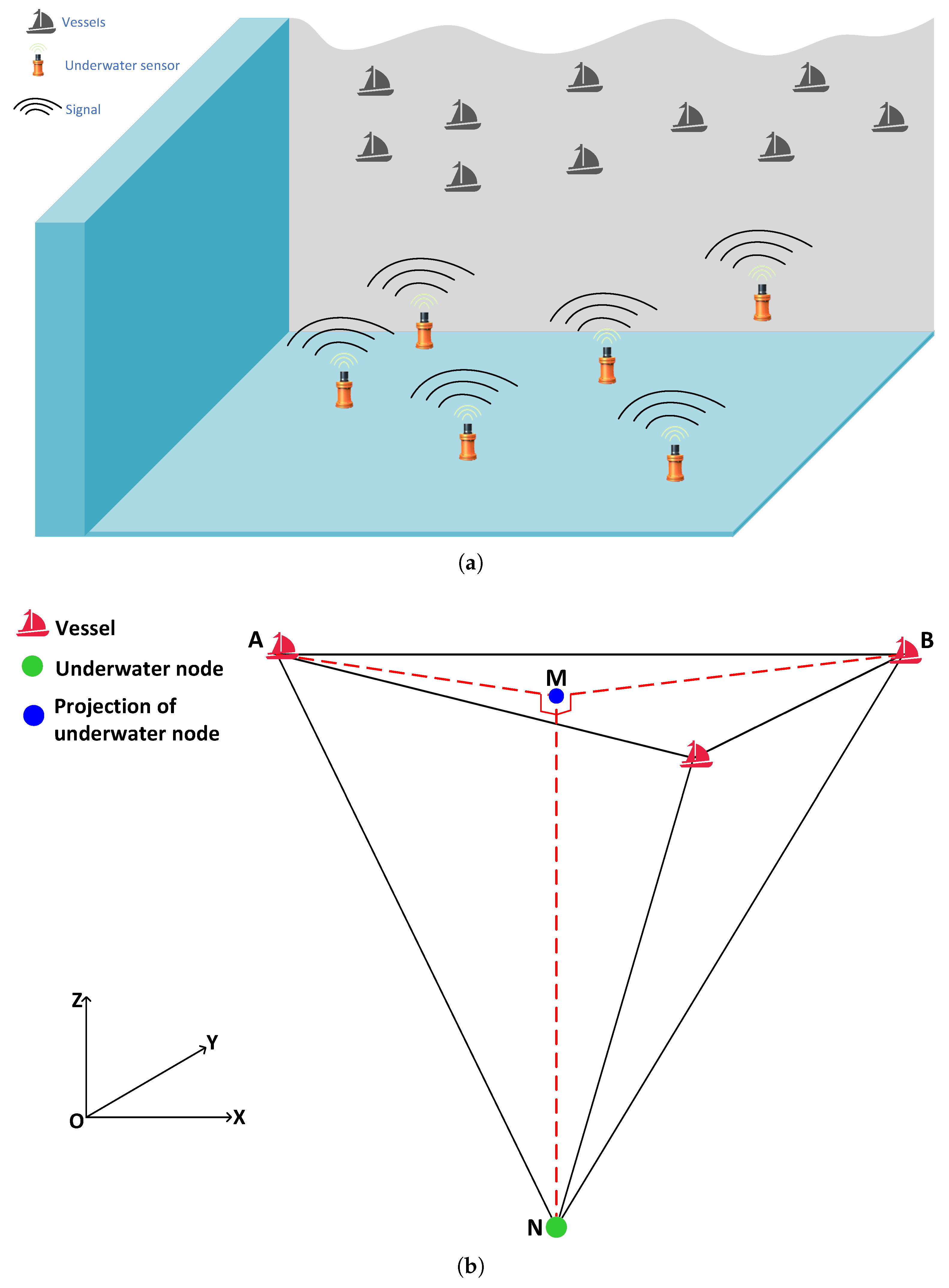
In the scenario of this algorithm, localization involves underwater sensor nodes and vessels. As shown in Figure 1a, the sensors are randomly distributed at various depths underwater to monitor different regions. These battery-powered sensors are equipped with pressure sensors for depth measurement and have a communication range of up to 1.5 km. Their primary function is to monitor the underwater environment and send localization requests, as they lack built-in localization capabilities. On the sea surface, the vessels are equipped with GPS modules, as well as communication and computational resources. They can receive signals from the sensor nodes and communicate with other vessels, with a communication range of up to 30 km.

During the localization process, underwater nodes transmit localization request messages containing their node $ID$ and timestamp $(ID,T_s)$. Upon receiving these messages, surface vessels record their current position P and the message arrival time $TD$, then compute the propagation time as $T=T_D-T_S$. The vessels subsequently broadcast the node ID, their recorded position, and the calculated propagation time $(ID,P,T)$. As shown in Figure 1b, vessels A and B receive the localization message from the underwater node N, record their respective positions at the time of reception, calculate the propagation times $T_A$ and $T_B$, and broadcast this information to other vessels.

For computational simplicity, underwater nodes are projected onto the sea surface, where the vessels are located, effectively reducing the three-dimensional problem to a two-dimensional one. As shown in Figure 1b, the underwater node N is vertically projected onto the sea surface, with the projection point labeled as M. Equipped with pressure sensors, the underwater nodes can measure water depth. By calculating the X-coordinates and Y-coordinates of point M, the precise position of the underwater node can be accurately determined.

As shown in Figure 1b, the geometric relationships of distances among A, B, N and M are defined as

$$\left\{\begin{array}{c}{D_{MN}}^2+{D_{AM}}^2={D_{AN}}^2\hfill \\ {D_{MN}}^2+{D_{BM}}^2={D_{BN}}^2\hfill \end{array}\right.$$

(1)

Thus, it can be obtained that

$${D_{AN}}^2-{D_{BN}}^2={D_{AM}}^2-{D_{BM}}^2$$

(2)

The speed of sound underwater depends on factors such as temperature, salinity, and depth. In this study, the localization area is in the same sea area, and vessels A and B are located on the same horizontal plane. Therefore, we can assume the sound velocities c are the same. Substituting this assumption into Equation (2) yields the following result:

$$\begin{array}{c}\hfill \begin{array}{cc}\hfill {(c\times T_{AN})}^2-{(c\times T_{BN})}^2& ={(c\times T_{AM})}^2-{(c\times T_{BM})}^2\hfill \end{array}\end{array}$$

(3a)

$$\begin{array}{c}\hfill \begin{array}{cc}\hfill T_{AN}^2-T_{BN}^2& =T_{AM}^2-T_{BM}^2\hfill \end{array}\end{array}$$

(3b)

It can be concluded that when the condition $T_{AN}=T_{BN}$ is satisfied, $T_{AM}=T_{BM}$ is also true. This implies that vessels A and B are located on the same circle with point M as its center. By calculating the coordinates of the circle’s center, the precise position of point M can be determined, which represents the position of the node.

3.2. Crowdsensing-Based Circle Center Calculation

Vessels employ a crowdsensing approach to collaboratively calculate localization upon receiving a request. Vessels with identical message transmission times are located on the same circle, centered at the sea surface projection of the underwater node. Varying transmission times result in the formation of multiple concentric circles. However, the spatiotemporal variability of real-world environments makes it challenging to identify vessels with perfectly identical transmission times. To mitigate this limitation, a threshold time difference $\mathsf{\Delta }t$ is introduced. If the transmission time difference between two vessels is less than $\mathsf{\Delta }t$, they are deemed to be positioned on the same circle.

As shown in Figure 2, vessels A through L receive localization messages from the underwater node, calculate the message propagation time, and broadcast the results. Each vessel identifies other vessels from the received messages whose propagation time difference is smaller than a predefined threshold $\mathsf{\Delta }t$, forming a “same-circle set”—a group of vessels considered to lie on the same circle centered at the underwater node’s projection on the sea surface. According to the concentric circle center theorem, the perpendicular bisectors of any two points on different concentric circles intersect at the circle’s center. Thus, if the same-circle set includes at least two vessels, they can collectively participate in the calculation of the circle’s center. The size of the same-circle set can be controlled by adjusting $\mathsf{\Delta }t$. A smaller $\mathsf{\Delta }t$ reduces localization errors, enhancing accuracy, but also decreases the number of vessels in the set, potentially limiting the localization coverage. Therefore, selecting an appropriate $\mathsf{\Delta }t$ is critical to achieving a balance between localization accuracy and coverage.

As illustrated in Figure 3a, when the number of vessels in the circular region $AB$ is three or more, vessel A identifies vessels B and C whose propagation time differences relative to A are less than $\mathsf{\Delta }t$. The perpendicular bisectors of $AB$ and $AC$, denoted as $MB$-$M1$ and $MC$-$M1$, respectively, are constructed, with $MB$ and $MC$ serving as their respective bases. The intersection point of these bisectors, labeled as $M1$, represents the center of the circle that encompasses A, B, and C. Accordingly, the following formula is derived:

$$\left\{\begin{array}{c}{y}_{M1}-{\displaystyle \frac{y_A+y_B}{2}}=-{\displaystyle \frac{x_B-x_A}{y_B-y_A}}\times (x_{M1}-{\displaystyle \frac{x_A+x_B}{2}})\hfill \\ y_{M1}-{\displaystyle \frac{y_A+y_C}{2}}=-{\displaystyle \frac{x_C-x_A}{y_C-y_A}}\times (x_{M1}-{\displaystyle \frac{x_A+x_C}{2}})\hfill \end{array}\right.$$

(4)

To overcome the limitation imposed by a minimum vessel count in the same-circle set, which prevents circle center calculation and results in localization failure when fewer than three vessels are present, we propose an optimized algorithm. As shown in Figure 3b, if the number of vessels in the same-circle set $AB$ falls below three, vessel A identifies vessel B, whose message propagation time difference with A is less than $\mathsf{\Delta }t$. Similarly, vessel E in the same-circle set $EF$ selects vessel F based on the same criterion. Perpendicular bisectors are then drawn for the line segments $AB$ and $EF$, denoted as $MB$-$M2$ and $EF$-$M2$, with their respective feet marked as $MB$ and $ME$. The intersection of these bisectors determines the circle center, referred to as $M2$. This optimized approach allows the circle center to be calculated using the following formula:

$$\left\{\begin{array}{c}{y}_{M2}-{\displaystyle \frac{y_A+y_B}{2}}=-{\displaystyle \frac{x_B-x_A}{y_B-y_A}}\times (x_{M2}-{\displaystyle \frac{x_A+x_B}{2}})\hfill \\ y_{M2}-{\displaystyle \frac{y_E+y_F}{2}}=-{\displaystyle \frac{x_E-x_F}{y_E-y_F}}\times (x_{M2}-{\displaystyle \frac{x_E+x_F}{2}})\hfill \end{array}\right.$$

(5)

In a similar manner, vessel B-L identifies the concentric circle set to which it belongs and selects pairs of vessels (excluding itself) within the set to construct perpendicular bisectors. The intersections of these bisectors are used to estimate the centers of the circles. However, due to uncertainties such as propagation delays and the $\mathsf{\Delta }t$ parameter, deviations exist between the estimated and actual positions of the circle centers, resulting in a set of estimated centers, as illustrated in Figure 2. To enhance localization accuracy, a clustering-based optimization algorithm is then employed to refine the results.

3.3. Density-Based Noise Removal Algorithm

The circle center set is determined by calculating the intersection points of perpendicular bisectors formed by connecting pairs of vessels within multiple concentric circle sets. However, some intersection points may deviate significantly from the true circle center due to uncertainties in the process. As shown in Figure 4, point O represents the true circle center, while $[SI,S2,S3,\dots ,S8]$ denote the eight vessels in the set, and $[A1,A2,A3,A4,A5]$ indicate the calculated centers. Propagation delays and the $\mathsf{\Delta }t$ parameter introduce positional deviations, resulting in vessels being slightly offset from the circle. For example, $S1$ and $S2$, as well as $S5$ and $S6$, are relatively far apart, whereas $S3$ and $S4$, along with $S7$ and $S8$, are closer together. When two vessels are very close—one inside the circle and the other outside (e.g., $S3$ and $S4$, or $S7$ and $S8$)—their bisectors’ intersection points with those of other vessels can deviate drastically from the true center, producing outliers such as $A1$, $A2$, $A3$, $A4$. These outliers substantially impact localization accuracy during clustering-based optimization. Therefore, it is essential to eliminate these anomalies before proceeding with the optimization process.

As shown in Figure 4, the outliers are sparsely distributed, while the normal calculated circle centers are densely clustered around the true circle center O. To address this issue, a Density-Based Noise Removal (DBNR) algorithm is introduced to efficiently eliminate these outliers. The DBNR algorithm consists of the following three steps:

• Determining whether neighboring points fall within the neighborhood range: First, calculate the distance from point m to other points using Equation (6). Then, substitute these results into Equation (7) to determine whether the points surrounding point m are within the neighborhood defined by the radius $eps$. If the elements in the matrix $D_{m\_Index}$ are greater than zero, the corresponding point is considered to be within the neighborhood of m; otherwise, it is not.

  $$D_m=\left[\begin{array}{c}{x}_{1m}\\ x_{2m}\\ ⋮\\ x_{nm}\end{array}\right]=\sqrt{{\left(\left[\begin{array}{c}{x}_1\\ x_2\\ ⋮\\ x_n\end{array}\right]-x_m\right)}^2+{\left(\left[\begin{array}{c}{y}_1\\ y_2\\ ⋮\\ y_n\end{array}\right]-y_m\right)}^2}m\in (1,2,\dots ,n)$$

  (6)

  $$D_{m_{I}ndex}=\left[\begin{array}{c}Inde{x}_{1m}\\ Inde{x}_{2m}\\ ⋮\\ Inde{x}_{nm}\end{array}\right]=sgn(eps-D_m)m\in (1,2,\dots ,n)$$

  (7)
• Neighbor count calculation: Determine the neighbor count $Num$ for point m within the $eps$-neighborhood based on the elements of the matrix $D_{m\_Index}$.
• Outlier Detection: Identify a point as normal if $Num>minPts$ (the minimum threshold for neighborhood points); otherwise, classified it as an outlier.

By utilizing the DBNR denoising algorithm, outliers in the set of centroids generated by crowdsourced sensing can be effectively removed, thereby enhancing localization accuracy. The denoising process of the DBNR algorithm is shown in Algorithm 1.

Algorithm 1 Density-based noise removal

Input: $Points,ϵ,minPTs$

Output: $Point{s}_{\mathrm{clean}}$

1: for $i=1$ to N do

2:     $Neighbors\leftarrow$ Find_Neighbors($Points$, i, $ϵ$)

3:     if length($Neighbors$) < $minPTS$ then

4:         $Poin{t}_{\mathrm{index}}\left(i\right)\leftarrow -1$

5:         continue

6:     else

7:         $Poin{t}_{\mathrm{index}}\left(i\right)\leftarrow 1$

8:     end if

9:     $Point{s}_{\mathrm{clean}}\leftarrow$ Data($Points\left(i\right)$, $Poin{t}_{\mathrm{index}}\left(i\right)$)

10: end for

3.4. Aggregation Optimization Algorithm

To calculate the coordinates of the circle center, a clustering optimization algorithm is employed. The DBNR algorithm is first applied to preprocess the circle center set. Subsequently, the centroid-based approximate triangulation (CBAT) clustering optimization algorithm is used to refine the circle center set, enabling precise localization.

Directly clustering all points in the circle center set would result in an excessively large clustering area. Therefore, it is crucial to narrow the clustering region. The CBAT algorithm achieves this by applying a triangulation-based approach to the points in the circle center set, effectively improving localization accuracy. Specifically, the algorithm selects any three points from the set to form a triangle and uses centroid-based point-in-triangle testing (CBPIT) to check whether an unknown node lies within the triangle. This process is repeated, forming new triangles and conducting point-in-triangle tests until all circle center points have been considered. Finally, the centroid of the overlapping region among the triangles passing the CBPIT test is computed to estimate the position of the unknown node.

The CBAT algorithm comprises two main steps: (1) Centroid-Based point-in test (2) CBAT clustering. These calculations are executed by the participating vessels involved in the localization process. The process of the CBAT algorithm is shown in Algorithm 2, with detailed steps to be elaborated in subsequent sections.

Algorithm 2 Centroid-based approximate triangulation

Input: $Point{s}_{clean}$

Output: $Estimating\_Position$

1: $Point\_N$ = Calculate_Centroid($Points$)

2: for $\mathrm{i}\leftarrow 1$ to size($Points$) do

3:     Triangle(i) = Triangulate($Points\left(i\right)$)

4:     if CBPIT(Triangle(i),$Point\_N$) == True then

5:         $Triangl{e}_{inSet}$ = Add(Triangle(i))

6:         continue

7:     end if

8: end for

9: $Overlap\_region$ = CBAT($Triangl{e}_{inSet}$)

10: $Estimating\_Position$ = Centroid($Overlap\_region$)

3.4.1. Centroid-Based Point-In Test

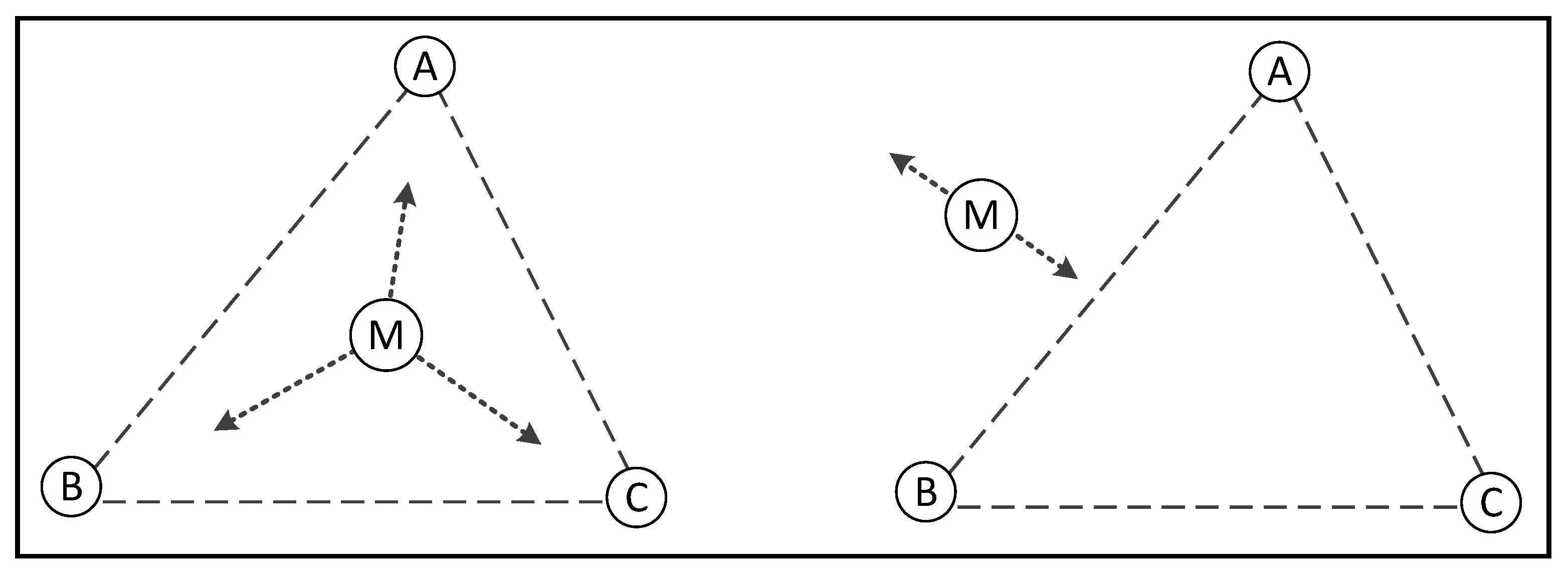
To determine whether a point M lies inside a triangle with vertices A, B, and C, the traditional point-in test is based on a set of geometric conditions. If these conditions are satisfied, point M is considered to be inside the triangle.

• Theory 1: If point M moves in any direction $\overrightarrow{d}$ from its initial position while satisfying the conditions of Equation (8), it can be determined that M lies within the triangle, as illustrated in the left panel of Figure 5.

  $$\forall \overrightarrow{d},\exists i\in \{1,2,3\},{\displaystyle \frac{d\left((\overrightarrow{M}+\mathrm{v}\overrightarrow{d}),{\overrightarrow{A}}_i\right)}{dt}}\ne 0$$

  (8)
  ${\overrightarrow{A}}_1,{\overrightarrow{A}}_2,{\overrightarrow{A}}_3$ denote the vectors corresponding to the vertices A, B, and C, respectively. $d((\overrightarrow{M}+\overrightarrow{\mathrm{v}d}),{\overrightarrow{A}}_i)$ represents the distance between point M and vertex $A_i$ along the direction of $\overrightarrow{d}$ as M moves, t represents the parameter of the distance that point M moves along the direction d. The derivative ${\displaystyle \frac{d((\overrightarrow{M}+\overrightarrow{vd}),{\overrightarrow{A}}_i)}{dt}}$ describes the rate at which the distance changes with respect to t.
• Theory 2: If there exists a direction $\overrightarrow{d}$ such that, when point M moves along this direction, Equation (9) is satisfied, then point M is located outside the triangle, as illustrated in the right panel of Figure 5.

  $$\exists \overrightarrow{d},\exists i\in \{1,2,3\},\left(\sum _{i=1}^3\left({\displaystyle \frac{d((\overrightarrow{M}+\mathrm{v}\overrightarrow{d}),{\overrightarrow{A}}_i)}{dt}}\right)=3\right)\mathrm{V}\left(\sum _{i=1}^3\left({\displaystyle \frac{d((\overrightarrow{M}+\mathrm{v}\overrightarrow{d}),{\overrightarrow{A}}_i)}{dt}}\right)=-3\right)$$

  (9)
  ${\overrightarrow{A}}_1,{\overrightarrow{A}}_2,{\overrightarrow{A}}_3$ denote the vectors corresponding to the vertices A, B, and C, respectively. $d((\overrightarrow{M}+\overrightarrow{\mathrm{v}d}),{\overrightarrow{A}}_i)$ represents the distance between point M and vertex $A_i$ along the direction of $\overrightarrow{d}$ as M moves, t represents the parameter of the distance that point M moves along the direction d. The derivative ${\displaystyle \frac{d((\overrightarrow{M}+\overrightarrow{vd}),{\overrightarrow{A}}_i)}{dt}}$ describes the rate at which the distance changes with respect to t.

Based on the above theories, point M can be determined to be either inside or outside the triangle if it satisfies either Theory 1 or Theory 2. However, exploring all possible directions from point M is computationally impractical. To address this limitation, we propose the following theory.

Theory 3: If there exists a point N sufficiently close to point M and N is inside the triangle, then M can also be considered to be inside the triangle.

According to Theory 3, determining whether M lies inside the triangle requires only finding a point N near point M that meets the conditions. The points in the circle center set are essentially estimates of the unknown node’s position. These estimates, though surrounding the actual position, exhibit some errors. To aggregate these points into a single representative localization point, a centroid algorithm is applied. By calculating the centroid N of the circle center set, N serves as the aggregated point that represents all circle centers or estimated positions. The computation of N is defined in Equation (10). The error between point N and the actual position is minimal, making N a reliable reference for determining whether M is inside the triangle. This approach constitutes an improved version of the traditional PIT test tailored to the current scenario, referred to as the CBPIT test.

$$(N_x,N_y)=\left({\displaystyle \frac{1}{n}}\sum _{i=1}^n{x}_i,{\displaystyle \frac{1}{n}}\sum _{i=1}^n{y}_i\right)$$

(10)

3.4.2. CBAT Clustering

Although the error between point N and the actual position is minimal, N is only the result of a preliminary clustering operation, providing sufficient accuracy to assist in determining whether point M lies within the triangle. To achieve higher localization accuracy, a more precise clustering method, known as CBAT clustering, is required.

The approximate triangulation method involves combining multiple points to form triangles and calculating the centroid of their overlapping regions. Points from the circle center set are iteratively combined to construct triangles, which are subjected to CBPIT testing. Triangles passing the test are then processed using the approximate triangulation method. As illustrated in Figure 6, the process of CBPIT testing and approximate triangulation is repeated until all possible triangle combinations from the circle center set are exhausted. The centroid of the final overlapping shaded region is then computed to determine the final estimated position of the localization point. In Figure 6, the blue point represents the centroid of all points in the circle center set (referred to as the “N” point in Theory 3). The shaded region corresponds to the overlapping area of triangle combinations that pass the CBPIT test, and the black point indicates the final estimated position.

3.5. Analysis

This section provides a detailed explanation of the designed algorithm. First, the overall network model is introduced, and the positioning model is elaborated. By projecting node positioning from three-dimensional space to a two-dimensional plane, the node positioning process is simplified. Then, the crowdsensing-based center calculation algorithm is explained in detail. The center calculation model utilizes the concentric circle principle to determine whether ships are on the same concentric circle by analyzing the time difference in receiving node positioning requests from the ships, thereby calculating a set of centers, i.e., the initial node position set. Next, the density-based denoising algorithm is introduced in detail. During the crowdsensing process, positioning noise points may arise due to ship dynamics, environmental complexity, and time thresholds, which affect the positioning results. However, since anomaly points are generally sparsely distributed, a density-based denoising algorithm is employed to remove these noise points. Finally, the aggregation optimization algorithm is explained in detail. After processing the center set with the denoising algorithm, the CBPIT (Circumcircle-Based Point Inclusion Test) is first used to determine whether a point lies within a triangle. Then, the triangles that pass the test are reduced in the aggregation area using an approximate triangulation approach, and CBAT (Convex Boundary Approximation Technique) aggregation is performed to calculate the final node position; the overall process of CSUL is shown in Algorithm 3.

The node positioning algorithm designed in this paper has the following advantages: (1) no need to deploy beacon nodes separately in underwater sensor networks; (2) no ranging is required; (3) underwater nodes only send a single message during the positioning process, saving energy. However, the current algorithm is only suitable for scenarios with a large number of ships, as it imposes certain requirements on the number of ships around the node. If the number of ships is too small, it may lead to increased computational errors.

Additionally, the current algorithm is suitable not only for static node positioning but also for dynamic node positioning. During the positioning process, underwater nodes only send a single positioning request message and do not require information exchange with ships. The node position calculated by the algorithm corresponds to the time when the node sends the positioning request message. Even if the node moves, it will not affect the positioning process. If the underwater node moves quickly, the node only needs to send multiple positioning requests to update its position multiple times.

Algorithm 3 Crowdsensing-based underwater localization

Input: $Points,ϵ,minPTs$

Output: $Estimating\_Position$

1: for $i=1$ to N do

2:     $Neighbors\leftarrow$ Find_Neighbors($Points$, i, $ϵ$)

3:     if length($Neighbors$) < $minPTS$ then

4:         $Poin{t}_{\mathrm{index}}\left(i\right)\leftarrow -1$

5:         continue

6:     else

7:         $Poin{t}_{\mathrm{index}}\left(i\right)\leftarrow 1$

8:     end if

9:     $Point{s}_{\mathrm{clean}}\leftarrow$ Data($Points\left(i\right)$, $Poin{t}_{\mathrm{index}}\left(i\right)$)

10: end for

11: $Point\_N$ = Calculate_Centroid($Point{s}_{clean}$)

12: for $\mathrm{i}\leftarrow 1$ to size($Point{s}_{clean}$) do

13:     Triangle(i) = Triangulate($Point{s}_{clean}\left(i\right)$)

14:     if CBPIT(Triangle(i),$Point\_N$) == True then

15:         $Triangl{e}_{inSet}$ = Add(Triangle(i))

16:         continue

17:     end if

18: end for

19: $Overlap\_region$ = CBAT($Triangl{e}_{inSet}$)

20: $Estimating\_Position$ = Centroid($Overlap\_region$)

4. Experimental Results and Analysis

To evaluate the proposed localization algorithm, MATLAB R2019b simulations were conducted to compare the performance of four approaches: DV-Hop, CBAT clustering, CBAT_without_DBNR clustering, and Cen-Agg clustering. To mitigate the impact of random errors, each simulation was repeated 50 times, and the average results were used as the final outcomes. The performance of the four algorithms was evaluated based on three key metrics: localization coverage, localization error, and average energy consumption. The vessel location data used in the simulations were sourced from the http://www.ships66.com/ website, as shown in Figure 7. Specifically, the positions of 50 vessels were selected within the longitude range of $122.{1827}^{\circ }$ E–$122.{2118}^{\circ }$ E and the latitude range of $29.{9329}^{\circ }$ N–$29.{9506}^{\circ }$ N. A cubic region measuring 500 m × 500 m × 500 m was defined within this area, where 200 sensor nodes were randomly deployed. All nodes in the network were assumed to be stationary. The simulations were conducted by varying the communication range of the nodes and the $\mathsf{\Delta }t$ parameter used in circle center calculations. The detailed simulation parameters are presented in

Table 1. Experimental parameters.

Parameters	Values
Ship Location Area	$122.{1827}^{\circ }$ E –$122.{2118}^{\circ }$ E, $29.{9329}^{\circ }$ N –$29.{9506}^{\circ }$ N
Time Error	[0.001 s, 0.002 s, 0.003 s, 0.004 s, 0.005 s, 0.006 s, 0.007 s, 0.008 s]
Communication Range	[500 m, 600 m, 700 m, 800 m, 900 m, 1000 m]
Number of Nodes	200
Simulation Count	50

.

4.1. Localization Coverage

Localization coverage refers to the ratio of successfully localized nodes to the total number of nodes in the sensor network, as shown in Equation (11). Here, C represents the localization coverage, $N_{suc}$ represents the number of successfully localized nodes, and $N_{total}$ represents the total number of nodes in the sensor network.

$$C={\displaystyle \frac{N_{suc}}{N_{total}}}$$

(11)

As shown in Figure 8, the node communication range increases incrementally from 900 m to 1400 m. The experimental results indicate that, with the same time error $\mathsf{\Delta }t$, for the CBAT algorithm, as the communication range increases, the number of vessels receiving localization requests gradually increases, and the node localization coverage also grows, initially rising and then stabilizing at a peak value. For the DV-Hop algorithm, as the communication range expands, the number of vessels it can receive and the number of nodes it can interact with both increase, leading to a gradual rise in its localization coverage. When the communication range is 900 m, since DV-Hop is a multi-hop algorithm, it can communicate with more nodes through node connectivity when the communication range is sufficient. Therefore, its localization coverage is higher than the CBAT algorithm. When the communication range is greater than or equal to 1000 m, and the time error $\mathsf{\Delta }t$ is 0.005 s or 0.006 s, the number of vessels that nodes can communicate with increases in the CBAT algorithm. As a result, the localization coverage of the CBAT algorithm is higher than that of the DV-Hop algorithm, with the coverage reaching 98% when $\mathsf{\Delta }t$ is 0.006 s.

As shown in Figure 9, the time error $\mathsf{\Delta }t$ increases incrementally from 0.001 s to 0.006 s. The experimental results indicate that, under the same communication range, as the time error $\mathsf{\Delta }t$ increases, the number of vessels participating in localization within the same region also gradually increases. As a result, the node localization coverage of the CBAT algorithm increases, initially rising and then stabilizing at the peak value. When the time error $\mathsf{\Delta }t$ is 0.006 s and the communication range is 900 m or 1000 m, the localization coverage of the CBAT algorithm exceeds 90%, with the highest coverage approaching 100% when the communication range is 1000 m.

4.2. Localization Error

Localization error refers to the difference between the estimated position calculated by the algorithm and the true position. The chosen localization error metric in this paper is the root mean square error (RMSE), and its calculation method is given in Equation (12). In the formula, N represents the total number of nodes in the network, $X{t}_i$ and $Y{t}_i$ represent the true x and y coordinates of the node, and $X{e}_i$ and $Y{e}_i$ represent the estimated x and y coordinates of the node calculated by the algorithm.

$$RMSE=\sqrt{{\displaystyle \frac{1}{N}}\sum _{i=1}^n\left[{\left(X{t}_i-X{e}_i\right)}^2+{\left(Y{t}_i-Y{e}_i\right)}^2\right]}$$

(12)

Figure 10 illustrates the root mean square error (RMSE) of node localization under varying time errors ($\mathsf{\Delta }t$) for CBAT clustering, CBAT_without_DBNR clustering, and Cen-Agg clustering, as a function of communication range. The results demonstrate that, for a given time error ($\mathsf{\Delta }t$), the CBAT algorithm consistently achieves the lowest localization error. As the communication range increases, the number of vessels participating in the localization process grows, leading to a gradual reduction in localization error, which eventually stabilizes. When the node localization coverage reaches its maximum (i.e., communication range R = 100 m and time error $\mathsf{\Delta }t$ = 0.006 s), the localization error of CBAT stabilizes at approximately 5 m. By contrast, CBAT_without_DBNR clustering and Cen-Agg clustering yield higher localization errors under the same conditions. Among the three methods, CBAT_without_DBNR clustering exhibits the largest localization error, with a difference of approximately 15 m compared to CBAT clustering when the localization coverage is maximized. This finding underscores the significant impact of noise points on localization accuracy, as detailed in Section 3. The DBNR denoising algorithm proposed in Section 3 effectively addresses this issue by mitigating the influence of noise points. Furthermore, Cen-Agg clustering achieves a localization accuracy that is better than CBAT_without_DBNR clustering but inferior to CBAT clustering. While Cen-Agg clustering provides sufficient accuracy for the CBPIT testing of circle centers, it does not meet the precision requirements for final localization. Therefore, CBAT clustering is essential to achieve more accurate and reliable localization results.

As the DV-Hop algorithm’s localization error is unaffected by time errors and depends solely on the communication range, Figure 11 compares the localization errors of CBAT clustering, CBAT_without_DBNR clustering, and Cen-Agg clustering under maximum localization coverage ($\mathsf{\Delta }t$ = 0.006 s) with that of the DV-Hop algorithm across varying communication ranges. Figure 11 demonstrates that the localization errors of CBAT, CBAT_without_DBNR, and Cen-Agg clustering are significantly lower than those of the DV-Hop algorithm. Among these methods, the CBAT algorithm achieves the highest localization accuracy, with its error stabilizing at approximately 5 m. In contrast, the DV-Hop algorithm exhibits a decrease in localization error as the communication range increases, eventually stabilizing at around 70 m. This trend is attributed to the fact that a larger communication range allows more nodes to participate in the DV-Hop algorithm’s multi-hop process, thereby reducing localization errors. In summary, under the same communication range, the CBAT algorithm consistently demonstrates the highest localization accuracy.

Figure 12 compares the root mean square error (RMSE) of node localization for CBAT clustering, CBAT_without_DBNR clustering, and Cen-Agg clustering under varying communication ranges and time errors. Previous analyses suggest that increasing the time error leads to more vessels participating in localization within the concentric circle set. However, these vessels are farther from the circle’s circumference, which increases calculation errors in the estimated circle centers. As shown in Figure 12, for the same communication range, the localization errors of all three algorithms increase as the time error grows. Among these, the CBAT algorithm consistently achieves the smallest localization error. As the time error increases, the number of participating vessels also rises, which gradually reduces the node localization error and eventually stabilizes. At maximum localization coverage (i.e., communication range R = 1000 m and time error $\mathsf{\Delta }t$ = 0.006 s), the localization error of the CBAT algorithm stabilizes at approximately 5 m. In contrast, CBAT_without_DBNR clustering and Cen-Agg clustering exhibit significantly higher localization errors under the same conditions. The experimental results validate that the CBAT algorithm delivers the best performance, achieving the smallest localization error among the three approaches.

Table 2. Comparison of Figure 12 results.

Communication Range	500 m	600 m	700 m	800 m	900 m	1000 m
RMSE of CBAT ($\mathsf{\Delta }t=0.006$ s)	7.32271 m	10.55536 m	9.82653 m	8.79256 m	6.72342 m	5.79241 m
RMSE of Cen-Agg ($\mathsf{\Delta }t=0.006$ s)	7.97148 m	13.95205 m	14.80365 m	12.74287 m	15.1525 m	15.43707 m
RMSE of CBAT_without _DBRN ($\mathsf{\Delta }t=0.006$ s)	15.97148 m	17.95205 m	19.80365 m	19.74287 m	20.1525 m	21.43707 m

provides a detailed comparison of the RMSE for the three algorithms in Figure 12 at $\mathsf{\Delta }t$ = 0.006 s.

4.3. Energy Consumption

Energy consumption refers to the energy expended by sensor nodes during the localization process. In underwater environments, where energy resources are nearly impossible to replenish or replace, minimizing energy consumption is essential to prolong the lifetime of individual nodes and, by extension, the entire sensor network. The energy consumption of underwater sensor nodes consists of two primary components: data processing and data transmission. Data processing energy is primarily determined by the size of the data packet, whereas data transmission energy depends on the communication environment, transmission distance, and data packet size. Accordingly, the energy required to transmit a data packet from one node to another in underwater environments is described by Equation (13).

$$E=l{\epsilon }_{elec}+la{\left(f\right)}^d{d}^2$$

(13)

$$loga\left(f\right)=0.011{\displaystyle \frac{f^2}{1+f^2}}+4.4{\displaystyle \frac{f^2}{4100+f^2}}+2.75\times {10}^{-5}{f}^2+0.0003$$

(14)

In this context, l represents the size of the transmitted data packet, d denotes the transmission distance, and $a{\left(f\right)}^d$ refers to the transmission amplification coefficient derived from the free-space and multipath models during signal propagation. Due to the unique characteristics of acoustic signals compared to electromagnetic signals, the absorption coefficients for underwater signal propagation in both models are expressed as $a\left(f\right)$, where f represents the frequency of the acoustic signal. The absorption coefficient $a\left(f\right)$ is calculated using Thorp’s empirical formula [35,36], as shown in Equation (14). The experimental parameter settings are detailed in

Table 3. Energy consumption experimental parameters.

Parameters	Values
$l_{\mathrm{CBAT}}$	10 byte
$l_{\mathrm{DV}-\mathrm{Hop}}$	13 byte
${\epsilon }_{\mathrm{elec}}$	400 nJ/byte
f	1 kHz

.

Figure 13 compares the energy consumption of the CBAT localization algorithm and the DV-Hop algorithm under varying communication ranges. As detailed in this study, energy consumption primarily depends on the size of transmitted data packets and the communication range. Consequently, both algorithms show increased energy consumption with the expansion of the communication range, as illustrated in Figure 13. Under the same communication range, the CBAT algorithm demonstrates significantly higher energy efficiency than the DV-Hop algorithm. This efficiency stems from CBAT requiring only a single signal broadcast with a data packet size of 10 bytes, compared to the multi-hop broadcasting required by DV-Hop, which involves a data packet size of 13 bytes. Therefore, the CBAT algorithm consistently consumes considerably less energy than the DV-Hop algorithm. Specifically, under optimal conditions—when localization error is minimized and localization coverage is maximized (i.e., at a communication range of 1000 m)—the energy consumption of the CBAT algorithm remains below 10 J, substantially outperforming the DV-Hop algorithm.

Table 4. Comparison of Figure 13 results.

Communication Range	500 m	600 m	700 m	800 m	900 m	1000 m
CBAT energy consumption	2.5199 J	3.6345 J	4.9548 J	6.4819 J	8.2167 J	10.1602 J
DV-Hop energy consumption	9.8277 J	11.812 J	13.52652 J	15.16752 J	17.09072 J	19.8123 J

compares the energy consumption of the two algorithms in Figure 13 under different communication ranges. In summary, the CBAT algorithm offers superior energy efficiency, making it a more effective choice compared to the DV-Hop algorithm.

Table 5. Algorithm comparison.

Indicator	Localization Coverage	Localization Error	Energy Consumption
CBAT	High	Low	Low
Cen-Agg	-	Medium	-
CBAT_without_DBRN	-	High	-
DV-Hop	Medium	-	High

provides a detailed comparison of the four algorithms mentioned in the simulation experiments. It can be seen that the CBAT algorithm outperforms the other algorithms in all metrics.

5. Conclusions

This paper presents a crowdsensing-based underwater node localization algorithm tailored for the Internet of Vessels. In this approach, vessels collaboratively perform node localization through crowdsensing. The process begins with the node transmitting a localization request. Upon receiving the request, vessels broadcast it to nearby vessels, enabling the crowdsensing process. The localization problem is subsequently projected from a three-dimensional to a two-dimensional plane using concentric circle calculations, generating an initial set of potential node locations, referred to as the concentric circle center set. To improve localization accuracy and mitigate errors caused by vessel mobility, environmental complexity, and time thresholds, a DBNR denoising algorithm is introduced to remove noisy data points. Then, the CBAT clustering optimization algorithm is employed to aggregate the center set, completing the final node localization.

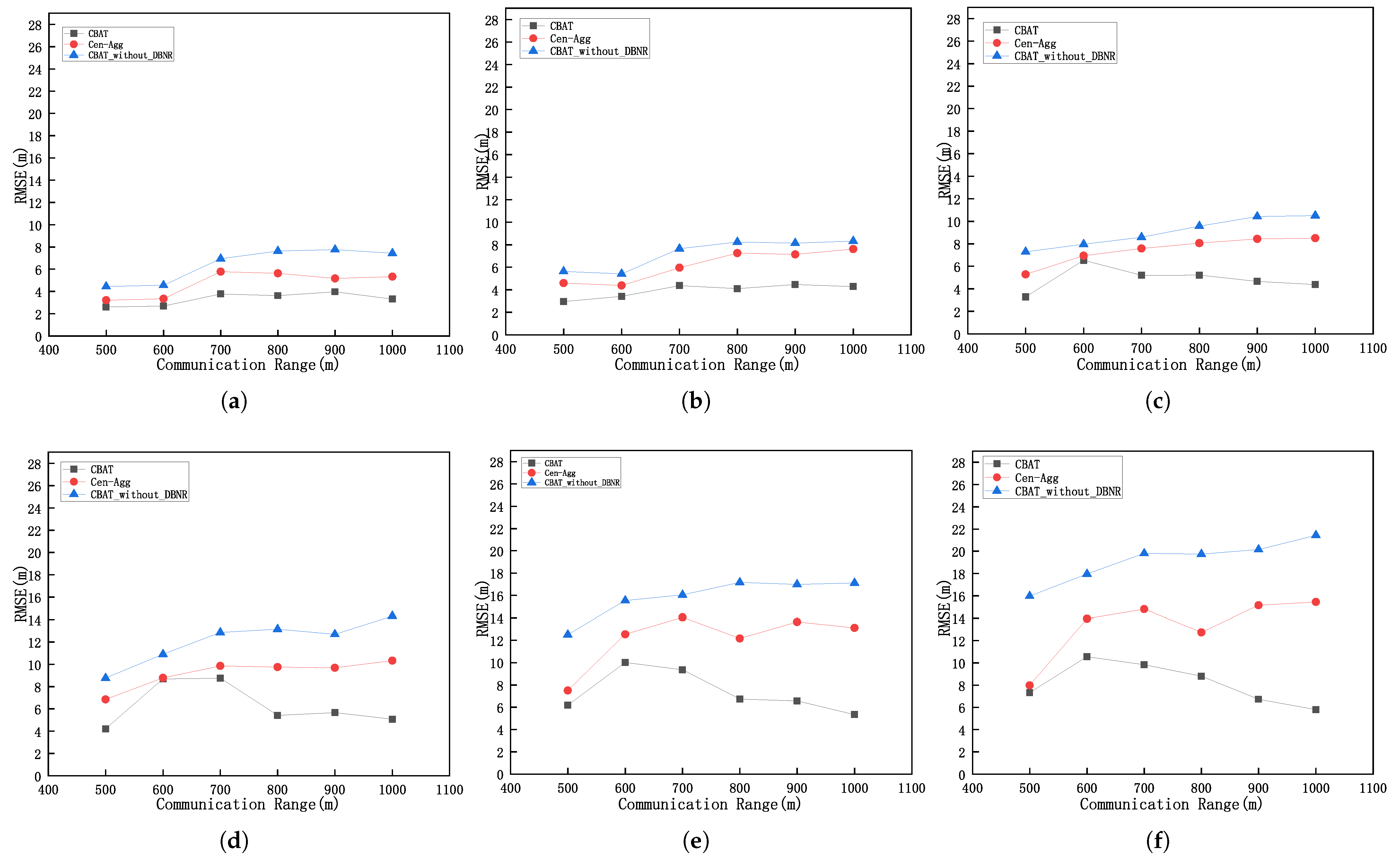
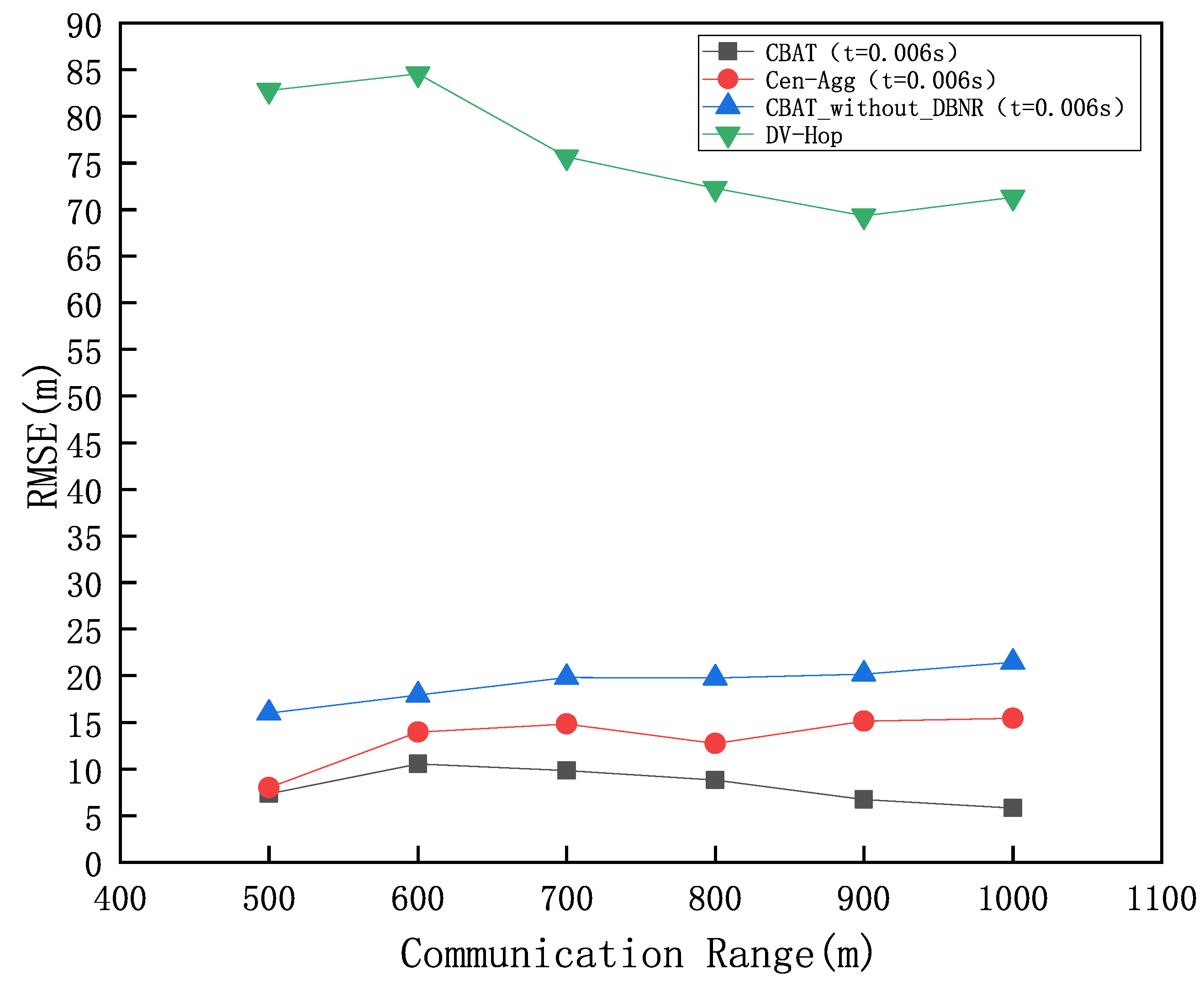
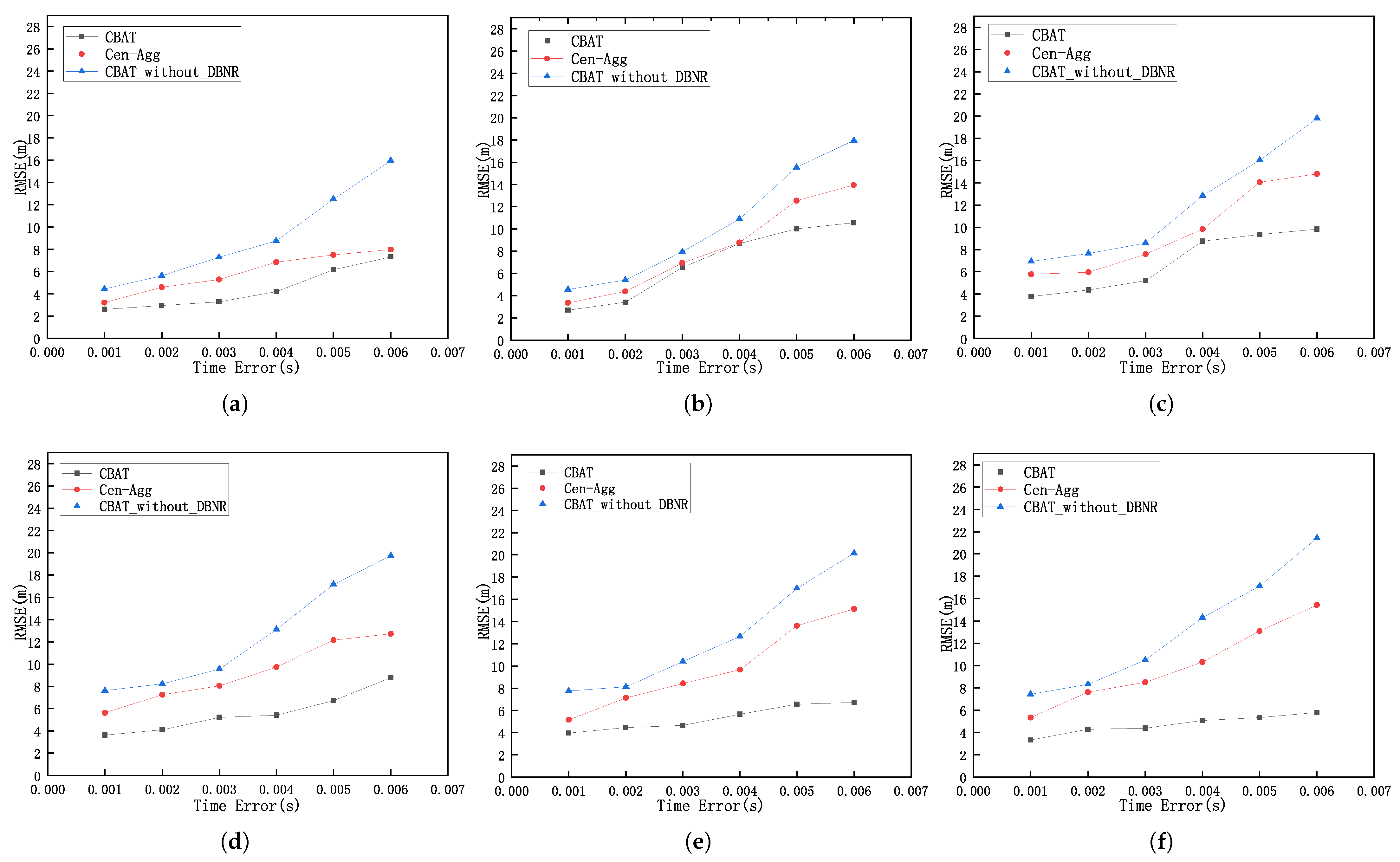
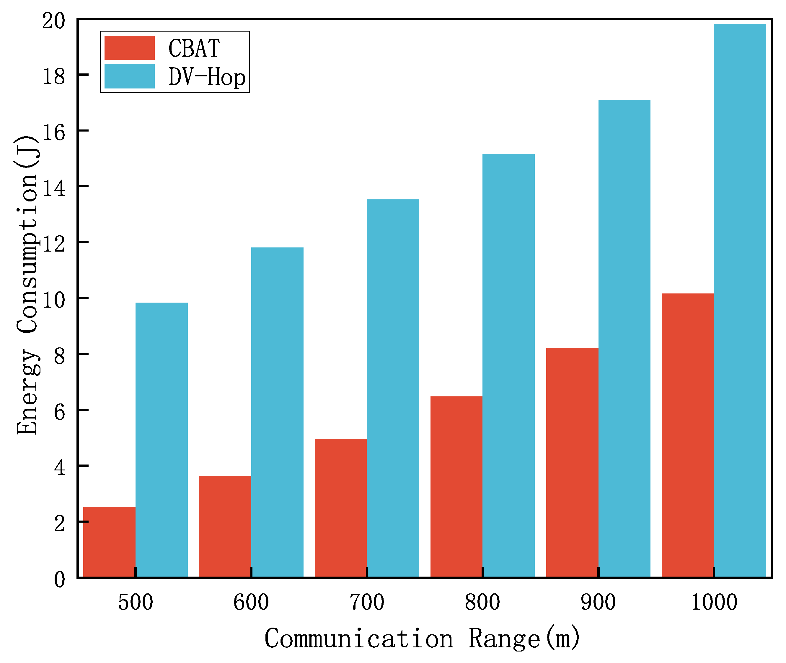
Experimental results indicate that the proposed algorithm achieves a localization coverage rate of up to 98% and significantly reduces localization errors compared to traditional algorithms such as DV-Hop and Cen-Agg. Furthermore, by leveraging vessels for computation and localization, the algorithm eliminates the computational and energy burdens on sensor nodes, substantially reducing communication energy consumption and effectively prolonging the network’s lifetime.