Nonlinear Compound Function-Based Course-Keeping Control for Ships in Rough Seas

Abstract

To ensure the safe navigation of ships in rough seas while reducing steering gear energy consumption and losses, a steering control system with small rudder output angles, low steering frequency, and high control performance was designed. A third-order closed-loop gain-shaping algorithm was employed in the development of the controller, with the ultimate control strategy derived by embedding a nonlinear compound function between the proportional derivative (PD) controller and the second-order oscillation link to enhance control effectiveness. A nonlinear Nomoto model of the “Yupeng” ship was employed for simulation validation. The simulation results illustrated a 14.5% improvement in overall control performance achieved by the proposed controller compared to a nonlinear feedback controller. The controller’s robustness was additionally validated through the application of the Norrbin ship model. The proposed controller enhances the stability of ships in rough seas, effectively limiting the maximum rudder angle during turns and reducing the average rudder angle and steering frequency during navigation. This design aligns with practical requirements for maritime operations in heavy weather, contributing significantly to the economic, safe, and efficient navigation of ships.

1. Introduction

With the continuous expansion of global trade and the growth of maritime transport [1], the safe navigation of ships has become particularly important [2]. Rough sea conditions such as high winds and waves pose greater challenges to the safe navigation of ships, making it extremely difficult to maintain a predetermined course. Scholars have studied the control of ship movements and unmanned vessels in rough seas [3,4]. However, in high winds and waves, ships not only need to steer frequently but sometimes even use large rudder angles to maintain stable navigation [5]. Therefore, the precise course control of ships is crucial for the economic and safe operation of ships, as well as for achieving effective motion control. While achieving precise control, it is also possible to reduce energy consumption [6,7].

Therefore, some scholars have explored and researched the problem of course-keeping control. Deng et al., in [8], proposed a model-based event-triggered control approach to track the activities of under-actuated surface ships to effectively control the closed-loop system. The method maximizes the reduction of learning parameters while achieving the tracking control of under-actuated surface vessels. Zhao et al., in [9], proposed a novel path-following control algorithm for surface vessels based on global course constraint (GCC) for the first time, and the path-following control algorithm takes the global course constraint as the goal. Min et al. in [10] suggested a second-order CGSA (closed-loop gain-shaping algorithm). First, a linear controller is designed using a second-order closed-loop gain-shaping algorithm. Then, the nonlinear modification technique is used to realize the final control law. The algorithm uses nonlinear modifications to reduce the rudder angle and steering frequency, providing innovative ideas for ship energy efficiency and environmental sustainability. Du et al., in [11], suggested a technique that integrates the Nussbaum gain function with a dynamic surface to address the challenge of maintaining the course under unknown control direction conditions, thereby enhancing the ship’s course control capability. Ren, in [12], proposed a method that uses T-S fuzzy approximation to handle uncertain ship dynamics and command filtering to simplify backstepping control for the ship course-keeping problem. Wang et al., in [13], proposed a CFD-based method, using naoe-FOAM-SJTU with an overset grid and a newly developed feedback controller, to simulate the free-running ONR Tumblehome ship model under course-keeping control in waves, addressing the problem of accurately predicting ship behavior in complex hydrodynamic conditions. Tuo et al., in [14], introduced a reliability-centered fixed-time non-singular terminal sliding mode control approach for the dynamic orientation of moored ships under conditions of uncertainties and unknown interferences. Zhang et al., in [15], designed an enhanced multiplicative event-triggered condition with a succinct estimation model, investigating the utilization of the multiplicative event-triggered mechanism for achieving a robust adaptive fault tolerance mechanism for unmanned surface vessels. Acanfora et al., in [16], proposed a method suitable for oceangoing ships, providing an autonomous routine for the avoidance of two dangerous phenomena involving excessive motions of the ship, e.g., the synchronous roll and the parametric resonance, both taking place in rough seas. Chen et al., in [17], proposed a method to generate information on ocean winds, wind-induced waves, and the strong Kuroshio western boundary current through modern weather and ocean models and then provide this information to ship maneuvering models to construct a numerical ship’s navigation system. Islam et al., in [18], proposed robust integral backstepping, synergetic, and terminal synergetic controllers for good course-keeping performance and reducing the energy consumption in course-keeping control for ships.

Most of the above studies focus on nonlinear modification technology and nonlinear feedback technology [19,20], as well as energy consumption and course-keeping under normal sea conditions [21,22]. However, when ships navigate in rough seas, the impact of high winds and waves can significantly reduce rudder effectiveness, severely affecting navigation stability and the effectiveness of course-keeping. Therefore, how to ensure safe and stable navigation through effective course control technology in rough seas remains a key issue in maritime technology research [23].

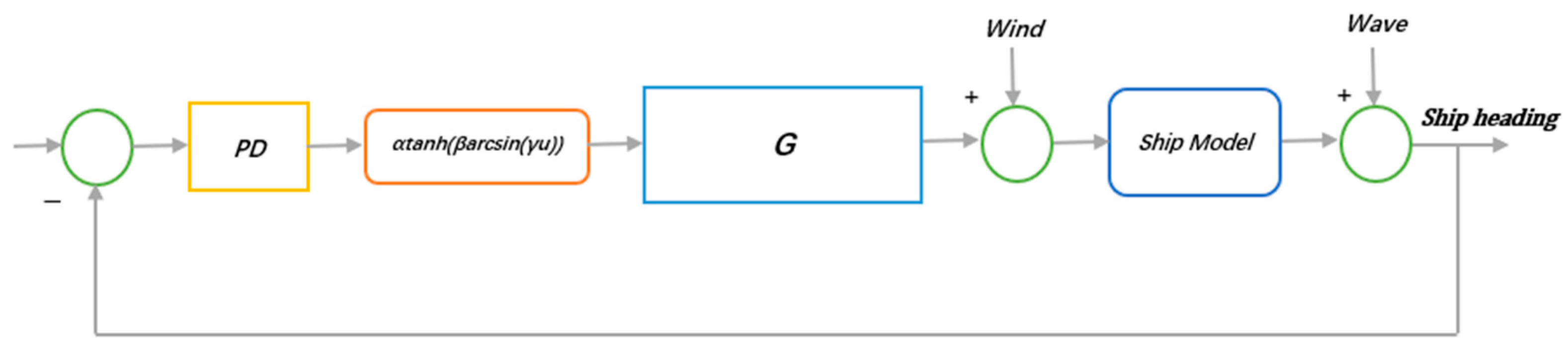
In this paper, the nonlinear composite function is integrated in series between the PD controller and the second-order oscillation link to propose a simple and robust control mechanism. Through comprehensive theoretical analysis and simulation experiments under different models, the effectiveness of the proposed controller is rigorously verified. The innovations presented in this paper can be summarized as follows:

(1)

For the first time, the controller has been enhanced using a nonlinear compound function to limit the maximum rudder angle during turns, thereby increasing the ship’s safety in rough seas.

(2)

A novel nonlinear embedded control strategy has been introduced, which not only reduces the average rudder angle and frequency of steering during navigation but also enhances course control accuracy.

The rest of this article is below. Section 2 describes the establishment of two mathematical models of ship motion: the Nomoto model and the Norrbin model. In Section 3, a controller based on a closed-loop gain-shaping algorithm is designed, and then a nonlinear composite function is embedded between the PD controller and the second-order oscillation link to improve, and the stability of the controller and the robustness of the system are demonstrated. 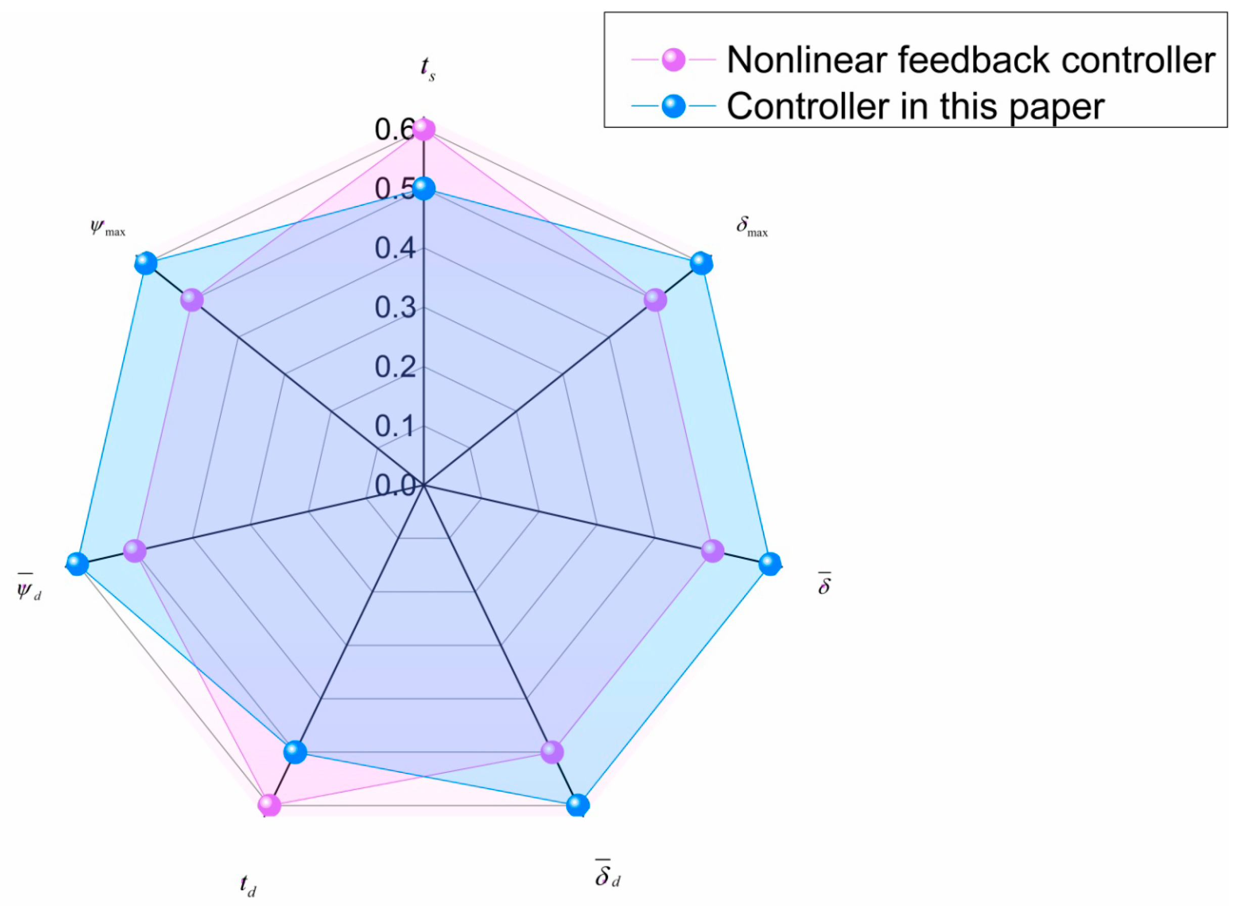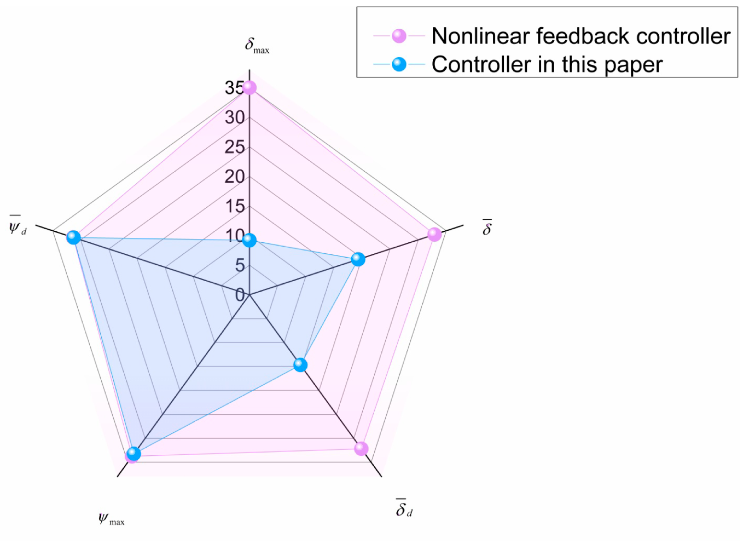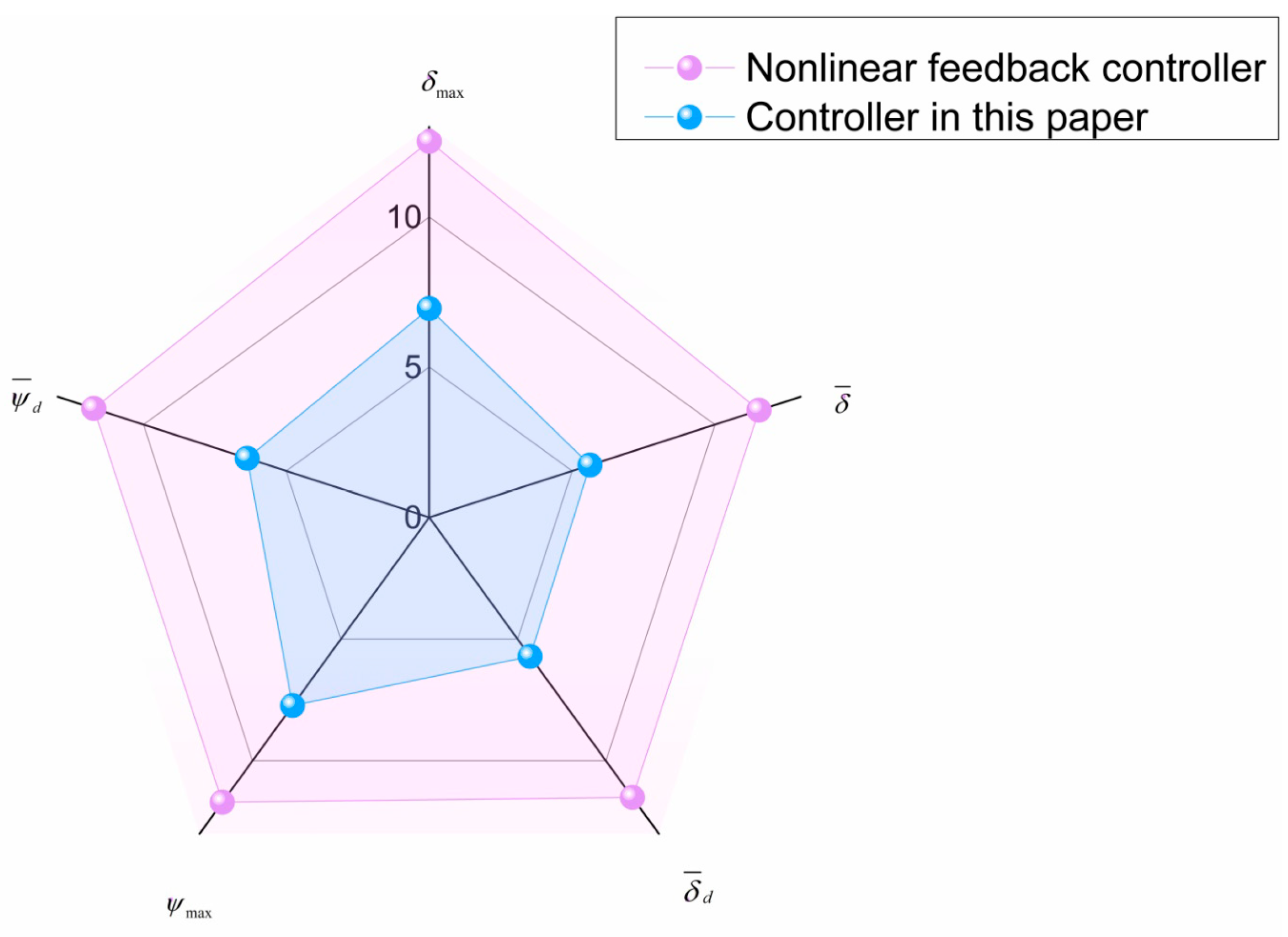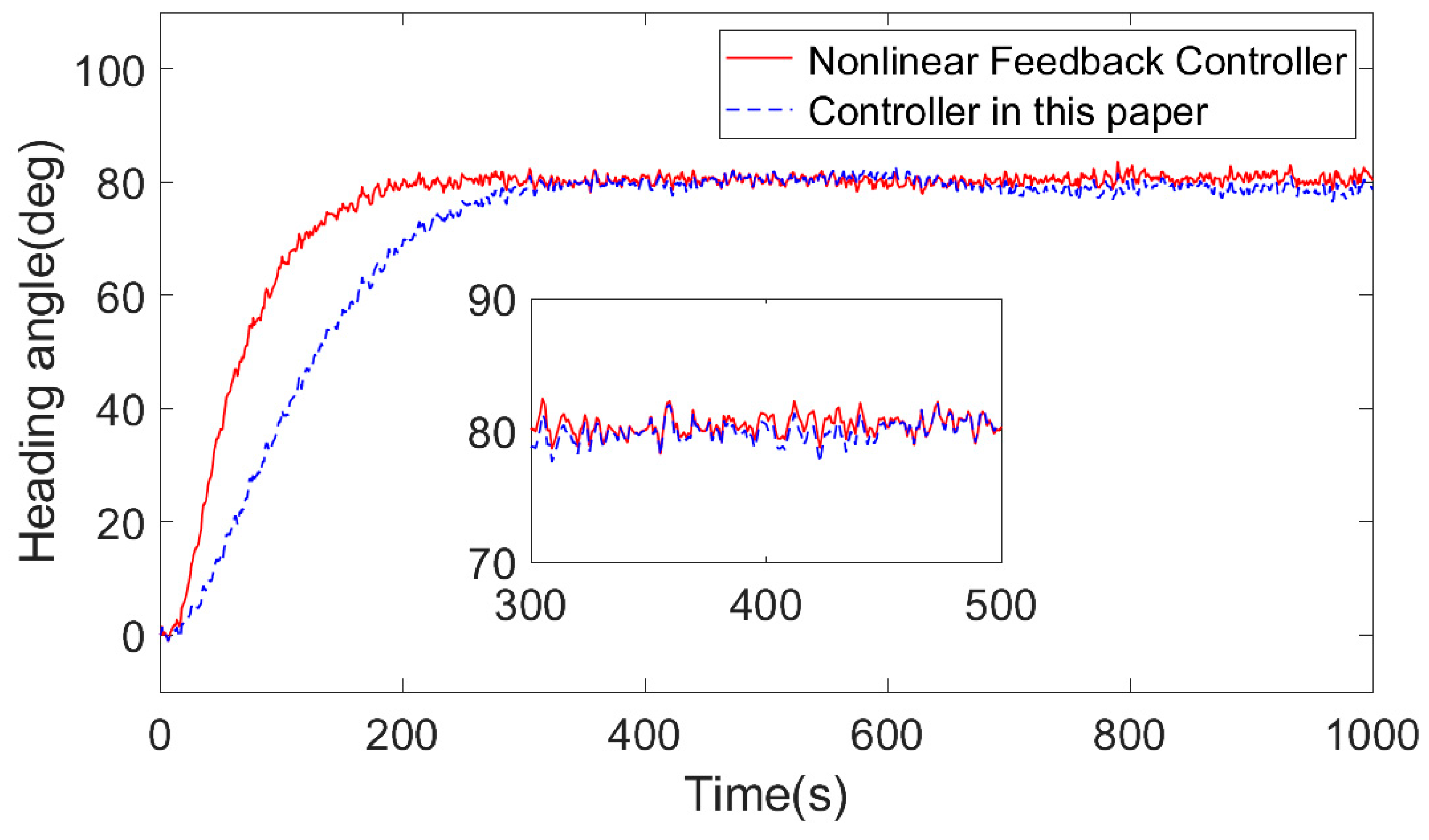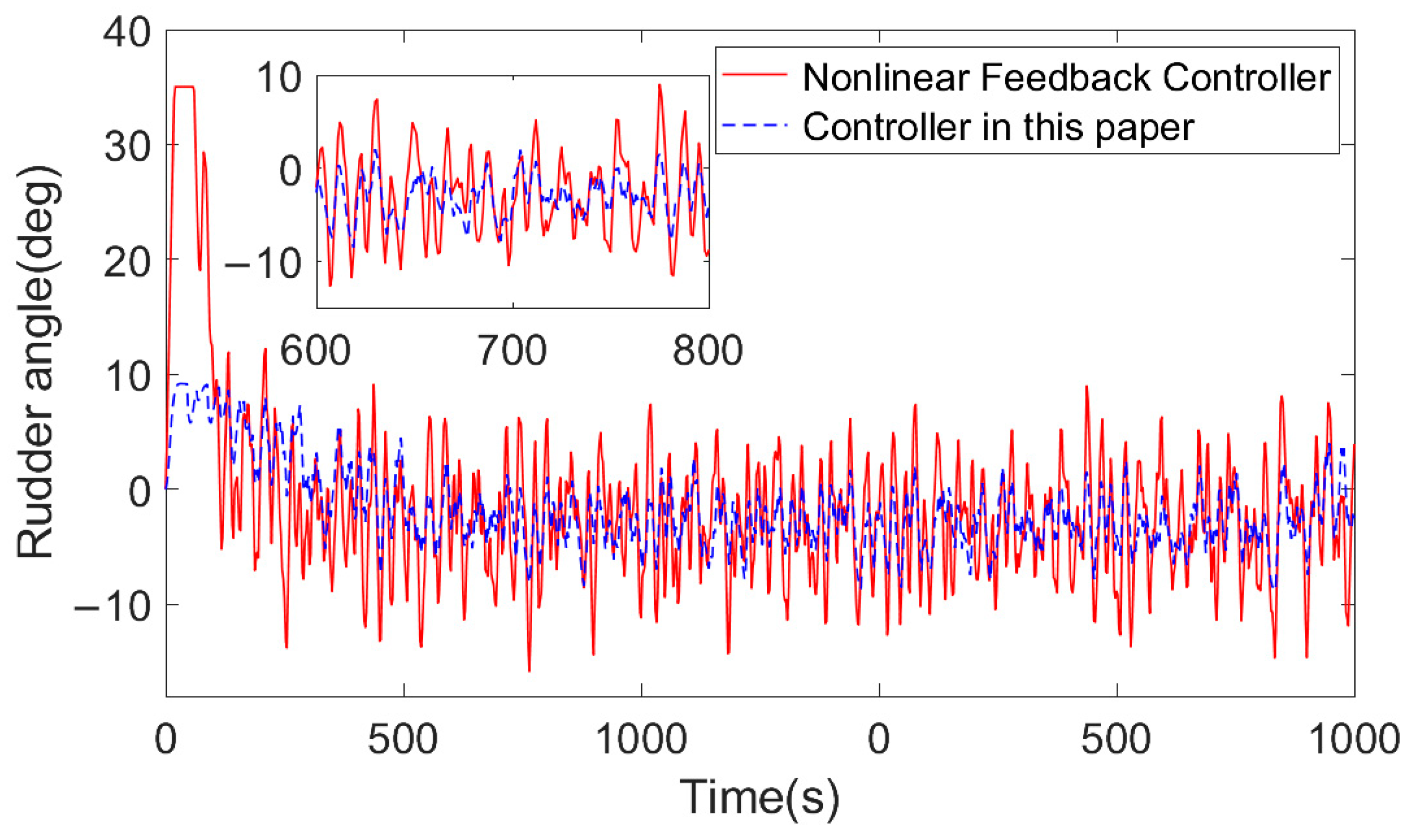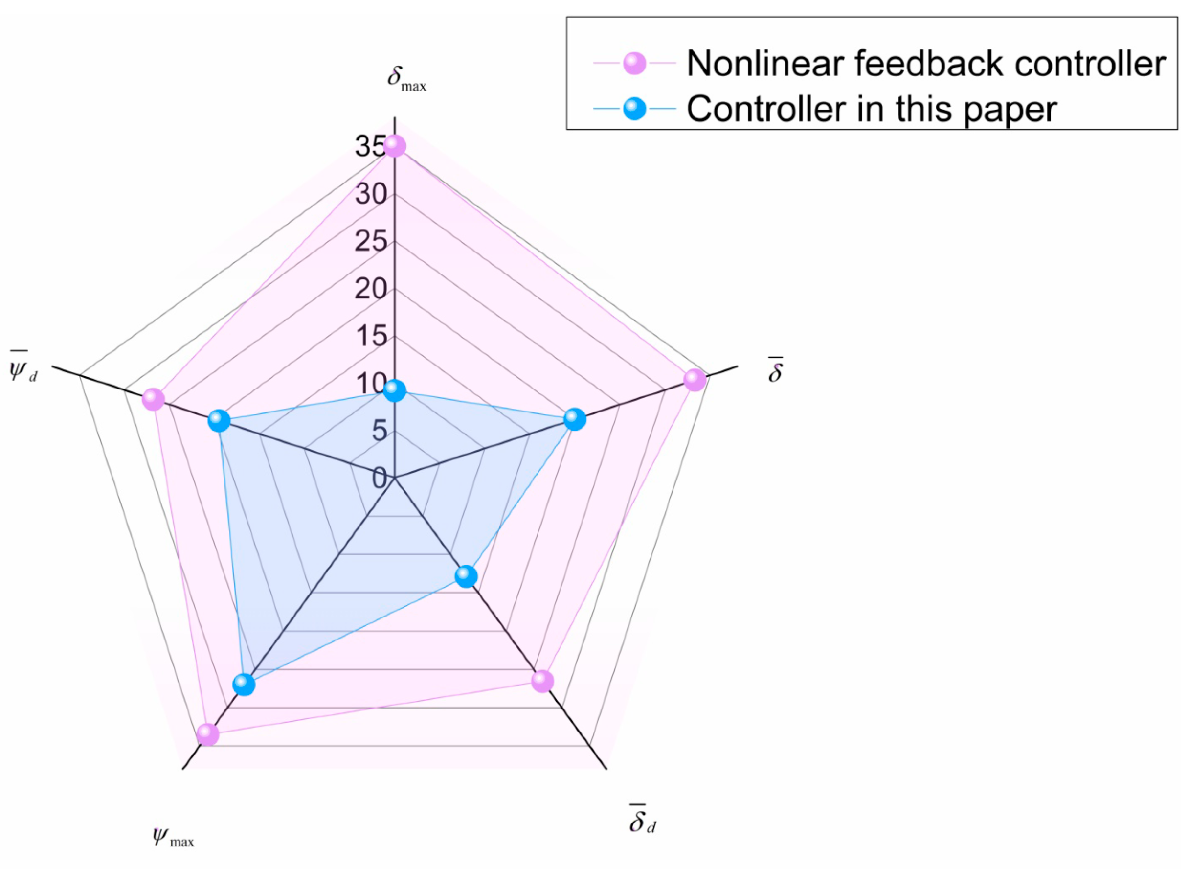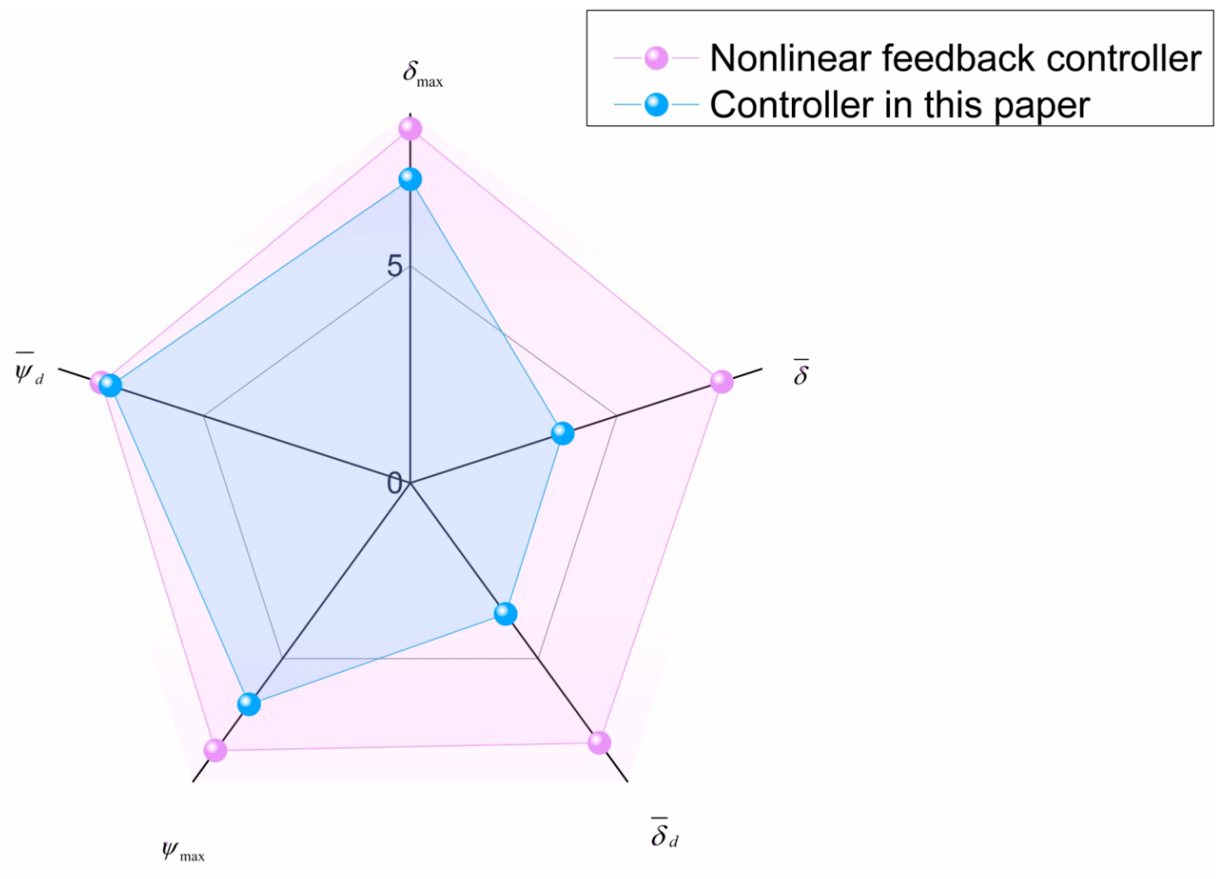Simulation experiments are carried out in Section 4, and the performance of the controller is represented by a radar chart. The selected performance index is calculated by the radar chart area, and the comprehensive index of the controller is obtained. The results show that the control effect of the controller effectively achieves the purpose of course control, reduces the rudder angle output, and achieves a good energy-saving effect.

2. Ship Motion Mathematical Model

2.1. Nonlinear Nomoto Mathematical Model for Ships

The mathematical model of ship motion selected in this paper is the response-type nonlinear Nomoto model [24]. The second-order Nomoto model is

$$\ddot{\psi }+{\displaystyle \frac{K_0}{T_0}}\left(A\dot{\psi }+B{\dot{\psi }}^3\right)={\displaystyle \frac{K_0}{T_0}}\delta$$

(1)

Additionally, $\dot{\psi }\to {\delta }_f:{\delta }_f=\left(A\dot{\psi }+B{\dot{\psi }}^3\right)-{\displaystyle \frac{1}{K_0}}\dot{\psi }=\left(A-{\displaystyle \frac{1}{K_0}}\right)\dot{\psi }+B{\dot{\psi }}^3$, where $\ddot{\psi }$ is the rate of yaw acceleration, $K_0$ is the turning index, $T_0$ is the following index, $\dot{\psi }$ is the yaw rate $\delta$ is the angle of rudder, and $A$ and $B$ are the nonlinear coefficients of the ship’s yaw rate. Ignoring the nonlinear terms in the equation results in a transfer function-type linear Nomoto model used for controller design: $G_{\psi \delta }={\displaystyle \frac{K_0}{s\left(T_{0}s+1\right)}}$.

2.2. Nonlinear Norrbin Mathematical Model for Ships

Norrbin introduced a simplified form of nonlinear fluid dynamics for analyzing ship parameter identification issues:

$$F_{NON}^{\prime }=\left(\begin{array}{c}{Y}_{NON}^{\prime }\\ N_{NON}^{\prime }\end{array}\right)=\left(\begin{array}{c}C{f}_Y\left(u,r\right)\\ C{f}_N\left(u,r\right)\end{array}\right)$$

(2)

where $f_Y\left(u,r\right)$ and $f_N\left(u,r\right)$ are expressions related to the yaw rate r and forward speed u, and the scale coefficient C is a dimensionless transverse flow coefficient, typically ranging from 0.3 to 0.8. The Norrbin model’s superiority lies in its clear theoretical basis and ease of application without requiring specific hull structure data except for the ship’s draft and length [25].

3. Controller Design

3.1. Controller Design Based on CGSA

In light of ship course-keeping control [26], we employ a closed-loop gain-shaping control algorithm (CGSA) that offers simplicity in solution and ensures excellent control performance and robust stability. This is also a simplified S/T mixed-sensitivity approach. Given the sensitivity function $S$ ($S=1/1+GK$, where $G$ represents the controlled object and $K$ is the controller) and the complementary sensitivity function $\left(T=GK/1+GK\right)$, we propose a CGSA. Figure 1 illustrates a typical S&T curve of singular value. To ensure robust stability, the spectrum of the closed-loop system must be low-pass, with a maximum singular value of 1, ensuring precise tracking of the reference signal without any steady-state error.

Assuming the closed-loop system’s bandwidth frequency is 1 (strictly speaking, it is the handover frequency), with the closure slope of the system’s closed-loop transfer function frequency set at −60 dB/dec, and assuming that the singular value curve of T closely approximates the spectral curve of a third-order inertial link with a peak singular value of 1, we obtain the following:

$${\displaystyle \frac{1}{{\left(T_{1}s+1\right)}^2}}={\displaystyle \frac{GK}{1+GK}}$$

(3)

By plugging the transfer function of the linear Nomoto model into Equation (3), the robust controller obtained from the third-order CGSA can be represented as follows [10]:

$$K=\left({\displaystyle \frac{T_{0}s}{K_0{T}_1}}+{\displaystyle \frac{1}{K_0{T}_1}}\right)\left({\displaystyle \frac{1}{T_1^2{s}^2+3T_{1}s+3}}\right)$$

(4)

During practical operations, the ship exhibits significant inertia, leading to prolonged control adjustments. A positive constant can be introduced to the proportional component of the PD link in Equation (4) to derive the controller as depicted in Equation (5):

$$K=\left({\displaystyle \frac{T_{0}s}{K_0{T}_1}}+{\displaystyle \frac{1}{K_0{T}_1}}+\rho \right){\displaystyle \frac{1}{T_1^2{s}^2+3T_{1}s+3}}$$

(5)

Introducing a constant $\rho$ within the proportional derivative controller framework, selecting a value between 1 and 10 for $\rho$ can significantly decrease the adjustment time of the system while maintaining stability [10].

To eliminate the impact of the net difference in CGSA control, a minute constant term can be introduced into the transfer function’s denominator to eliminate the effect of the net difference on ship control.

3.2. Controller Improvement Based on Nonlinear Modification

To simulate adverse sea conditions, a Beaufort level 8 wind and wave disturbance is incorporated into the controller for limitation. The rudder angle under the wind disturbance is calculated using the formula mentioned in [27]:

$${\delta }_{wind}=K^0\left({\displaystyle \frac{V_R}{V}}\right)\sin \left(\gamma \right)$$

(6)

Furthermore, the white noise substitution technique proposed by Kallstrom is employed in this study for processing. The white noise substitution technique proposed by Kallstrom is a method used to analyze and stabilize systems affected by noise and uncertainty. This technique involves replacing the original stochastic signals with white noise, allowing for a clearer assessment of system dynamics and performance under varying conditions. The deviation resulting from these white noises is directly proportional to the square of the absolute wind speed. The formula is as follows:

$${\sigma }_Y=0.2{\rho }_A{V}_T^2{\left|C_Y\left({\gamma }_R\right)\right|}^2{L}^2$$

(7)

$${\sigma }_N=0.2{\rho }_A{V}_T^2{\left|C_N\left({\gamma }_R\right)\right|}^2{L}^3$$

(8)

Here, ${\rho }_A$ is the air density, $L$ is the length of the ship, and $C_Y\left({\gamma }_R\right)$ and $C_N\left({\gamma }_R\right)$ are the dimensionless coefficients of wind force and wind moment, respectively.

The transfer function h(s) of the wave model obtained under the influence of an eight-level wind is given by Equation (9):

$$h\left(s\right)={\displaystyle \frac{1.3353s}{s^2+0.5153s+0.2655}}$$

(9)

In this paper, the function $\alpha \tanh \left(\beta \arcsin \left(\gamma u\right)\right)$ is chosen, which combines the hyperbolic tangent function and arcsine, modifying the linear control law (5). The function is primarily a gain regulator. $\alpha$, $\beta$, and $\gamma$ are used to adjust the amplitude of the input signal and the sensitivity of the response. By adjusting the $\alpha$, $\beta$, and $\gamma$ parameters, the controller can make a trade-off between stability and speed of response. Appropriate parameter selection can optimize the transition response of the system to avoid excessive response or excessive slowness. Due to the introduction of a nonlinear compound function in series between the PD controller and the second-order oscillation link, the final improved control law is nonlinear. The control system structure diagram is shown in Figure 2.

3.3. Stability Analysis

This paper uses the Nyquist stability criterion [28] in the frequency domain approach for analytical stability of a nonlinear compound function embedded third-order CGSA controller [29]. An analysis was conducted on the stability of the nonlinear Nomoto ship mathematical model along with a third-order CGSA controller [30]. A controller designed rooted in the Nomoto ship mathematical model alongside a third-order CGSA can yield the system’s open-loop transfer function as indicated by [25]:

$$\begin{gathered} G\left(s\right)={\displaystyle \frac{\left(T_{0}s+1+\rho K_0{T}_1\right)}{T_{1}s\left(T_{0}s+1\right)\left(T_1^2{s}^2+3T_{1}s+3\right)}} \\ ={\displaystyle \frac{1/T_1\left[s+\left(\rho K_0{T}_1+1\right)/T_0\right]}{s\left(s+1/T_0\right)\left[s+\left(3-\sqrt{3}j\right)/2T_1\right]\left[s+\left(3+\sqrt{3}j\right)/2T_1\right]}} \end{gathered}$$

(10)

Figure 3 illustrates the corresponding Nyquist plot.

Define N to represent the count of intersections of the curve with the passive real half-axis to the left of (−1, $j_0$), $N_{+}$ to denote the cross count from top to bottom to the left of (−1, $j_0$), $N_{-}$ to denote the cross count from bottom to top to the left of (−1, $j_0$), Z to stand as the number of poles of the closed-loop transfer function in the right half-plane, and P to denote the poles of the open-loop transfer function G(s) in the right half-plane. Z = P − ($N_{+}$ − $N_{-}$). Only when P = 0, $N_{+}$ = 0, $N_{-}$ = 0, and Z = P − ($N_{+}$ − $N_{-}$) = 0 can the closed-loop system be judged to be stable. Therefore, the proposed controller is stable when Z = 0.

Figure 3 shows the change curve of the controller in this paper when the frequency is $0\to +\infty$. It can be deduced that there are no poles on the right half-plane of the cyclic transfer function, that is, P = 0. The Nyquist curve drawn by the open-loop transfer function crosses the real axis from bottom to top through the left side of (−1, $j_0$). So, $N_{+}$ = 0, and $N_{-}$ = 0. Then,

$$Z=P-(N_{+}-N_{-})=0$$

(11)

(1) Expand to the first order using the Taylor series to obtain

$$\alpha \tanh \left(\beta \arcsin \left(\gamma u\right)\right)=\alpha \beta \gamma u$$

(12)

Impact on system stability: Consider a desired heading change represented as a step signal with a specified magnitude ${\psi }_r$. The Laplace transform’s final value law can be utilized to ascertain the steady-state value for the heading angle:

$$\begin{array}{l}\psi \left(\infty \right)=\underset{s\to 0}{\lim } s{\displaystyle \frac{G\alpha \beta \gamma K}{1+G\alpha \beta \gamma K}}{\displaystyle \frac{{\psi }_r}{s}}\\ =\underset{s\to 0}{\lim }{\displaystyle \frac{\frac{K_0}{s\left(T_{0}s+1\right)}\left(\frac{T_{0}s}{K_0{T}_1}+\frac{1}{K_0{T}_1}+\rho \right)\frac{\alpha \beta \gamma }{T_1^2{s}^2+3T_{1}s+3}}{1+\frac{K_0}{s\left(T_{0}s+1\right)}\left(\frac{T_{0}s}{K_0{T}_1}+\frac{1}{K_0{T}_1}+\rho \right)\frac{\alpha \beta \gamma }{T_1^2{s}^2+3T_{1}s+3}}}{\psi }_r\\ ={\psi }_r\end{array}$$

(13)

Consequently, the system’s steady-state behavior remains unaffected by the nonlinear modification technique and a zero-output steady-state error.

(2) Influence on the dynamic performance of the system: The transfer function of the unified frame of a closed-loop system is

$${\displaystyle \frac{\psi }{{\psi }_r}}={\displaystyle \frac{G\alpha \beta \gamma K}{1+G\alpha \beta \gamma K}}$$

(14)

When $\alpha \beta \gamma <1$, based on the CGSA, the open-loop transfer function GK of the system complies with the criterion of high gain at low frequencies and low gain at high frequencies. Thus, within the low-frequency domain, Equation (15) is consistent with the norm feedback system $GK/1+GK$ Despite the presence of $\alpha \beta \gamma$, changes in $\alpha \beta \gamma$ exert minimal influence on the dynamic functioning of the system.

(3) Influence on the controller output: Write the transfer function from input ${\psi }_r$ to controller output $\delta$:

$${\displaystyle \frac{\delta }{{\psi }_r}}={\displaystyle \frac{K\alpha \beta \gamma }{1+G\alpha \beta \gamma K}}$$

(15)

The introduction of $\alpha \beta \gamma$ leads to a decrease in the control output due to the more pronounced reduction in the numerator compared to the denominator in Equation (15). This leads to no poles in the right half-plane of the closed-loop transfer function, ensuring system stability.

3.4. Robustness Analysis

The purpose of this section is to explore the specific model perturbation forms of the CGSA. Based on the small gain theory and the $H_{\infty }$ mixed-sensitivity algorithm, we derive the fundamental disturbance model for the closed-loop gain-shaping algorithm.

Figure 4 illustrates a typical $H_{\infty }$ control problem. Within the framework of $H_{\infty }$ control, disturbances are integrated into the design concept through nonlinear composite functions to ensure that the robustness and stability of the control object set can be maintained while the controller is in place. For the traditional $H_{\infty }$ control problem in Figure 4, the small gain theory is first derived, and then the correlation between the model disturbance and the closed-loop transfer function of the system is obtained, as shown in Equation (16):

$${‖GK/\left(1+GK\right)\Delta ‖}_{\infty }={‖T\Delta ‖}_{\infty }<1$$

(16)

It can be seen from Equation (16) that the model disturbance $\Delta$ cannot be too large, so that the gain of the closed-loop transfer function $GK/\left(1+GK\right)$ is kept within a reasonable range, thus ensuring the stability of the closed-loop system.

By considering Figure 1 and the characteristics of the CGSA, we arrive at the following result [31]:

$$\begin{gathered} {‖T‖}_{\infty }\cdot {‖S‖}_{\infty }<1 \\ {‖TS‖}_{\infty }<1 \end{gathered}$$

(17)

Using Equations (16) and (17), we can obtain

$${‖\Delta ‖}_{\infty }={‖S‖}_{\infty }={‖1-T‖}_{\infty }$$

(18)

Based on Equation (18), the model disturbance form of the CGSA is similar to that of the sensitivity function S, and it should satisfy the corresponding conditions: ${‖\Delta ‖}_{\infty }<1$.

The foundation of the CGSA lies in the singular value curve derived from the weight function formulation within the $H_{\infty }$ robust control theory. Therefore, model perturbations are incorporated into the design, with the robust stability of the model validated through the $H_{\infty }$ theory. According to the findings of the small gain theory and the $H_{\infty }$ mixed-sensitivity method, it can be inferred that the model perturbation pattern in CGSA is consistent with the pattern of the sensitivity function S. This result is significant for determining the allowable magnitude of model disturbances when designing robust controllers using the CGSA.

As shown in Figure 5 Bode plot, the magnitude of S is significantly lower than 0 dB at low frequencies. This indicates excellent disturbance rejection capabilities in this frequency range. The peak magnitude of S, which is related to the maximum sensitivity to disturbances, appears to be around 0 dB. This implies that the system does not amplify disturbances significantly at any frequency.

The magnitude of T is close to 0 dB at low frequencies, indicating good tracking performance. At higher frequencies, the magnitude of T rolls off, providing noise attenuation and ensuring robustness against high-frequency uncertainties. The peak magnitude of T is also around 0 dB, which ensures that the system remains stable even with some modeling errors or uncertainties.

Remark 1.

In this section, we use the third-order CGSA to design a linear controller. The third-order CGSA itself has a simple form. A nonlinear compound function is connected between a traditional PD controller and a second-order oscillator, ensuring the final control law form, which makes the controller easy to implement.

Remark 2.

Embedding the nonlinear compound function into the third-order CGSA can enhance the response of the ship control system. This technology achieves more precise and gentle control in rough seas by adjusting the output rudder angle, reducing steering frequency and control input. It can enable ships to sail more safely and with greater energy savings in harsh sea conditions.

4. Simulation Experiments

In this section, the simulation object is the “Yupeng” practice ship of Dalian Maritime University, and the controller’s efficacy is validated through the application of the Simulink toolbox. This paper proposes a nonlinear compound function embedded in the third-order CGSA controller, which is compared with the nonlinear feedback controller mentioned in reference [13].

Table 1. Particulars of “Yupeng” ship.

Parameter	Unit	Parameter Value
$L$	$\mathrm{m}$	189
$B$	$\mathrm{m}$	27.8
$X_c$	$\mathrm{m}$	−1.8
$A_{\delta }$	${\mathrm{m}}^2$	38
$V$	$\mathrm{k}\mathrm{n}$	17.26
$\nabla$	${\mathrm{m}}^3$	42,293.0
$C_b$	/	0.72
$d_m$	$\mathrm{m}$	11

displays the important parameters of the “Yupeng” ship. From these parameters, $K_0$ = 0.38, $T_0$ = 298.44, $A$ = 11.98, and $B$ = 24,095.52 are derived. Additionally, take the value $\alpha =0.48$, $\beta =2.6$, and $\gamma =0.5$. The maximum rudder angle is set to 35° with a rudder speed cap of 5°/s.

To examine system robustness, the experiment was carried out under severe sea conditions, with the wind force at Beaufort level 8, the set heading of the ship during simulation at 080°, the simulation time set to 1000 s, and the fixed step length set to 1. Simulation experiments were conducted under the nonlinear Nomoto and Norrbin models, respectively.

To facilitate the comparison of the effects of the two controllers, this paper selects five indicators: delay time $t_d$, setting time $t_s$, and ${\psi }_{\max }$, ${\overline{\psi }}_d$, $\overline{\delta }$, ${\overline{\delta }}_d$, and ${\delta }_{\max }$ in classical control theory.

We define the following:

$${\psi }_{\max }=\max \left|{\psi }_r-\psi \left(t\right)\right|$$

(19)

$${\overline{\psi }}_d={\displaystyle \frac{1}{n}}{\displaystyle \sum _{t=0}^{n-1}\left|{\psi }_r-\psi \left(t\right)\right|}$$

(20)

$$\overline{\delta }={\displaystyle \frac{1}{n}}{\displaystyle \sum _{t=0}^{n-1}\left|\delta \left(t\right)\right|}$$

(21)

$${\overline{\delta }}_d={\displaystyle \frac{1}{n}}{\displaystyle \sum _{t=0}^{n-1}\left|\delta \left(t+1\right)-\delta \left(t\right)\right|}$$

(22)

$${\delta }_{\max }=\max \left|\delta \right|$$

(23)

${\psi }_{\max }$ and ${\overline{\psi }}_d$ assess the system’s response performance, while ${\delta }_{\max }$, $\overline{\delta }$, and ${\overline{\delta }}_d$ evaluate the energy consumption and smoothness of the control algorithm.

4.1. Simulation Experiment Based on Nonlinear Nomoto Model

Through simulation experiments through Simulink, the controller mentioned under the nonlinear Nomoto model and the heading simulation control effect of the controller in this paper can be obtained as shown in Figure 6, and the steering situation is shown in Figure 7.

The results calculated from the heading control effect diagram and steering situation diagram are shown in

Table 2. Controller parameters based on the Nomoto model.

Controller\Parameters	${\mathit{t}}_{\mathit{s}}\left(\mathit{s}\right)$	${\mathit{t}}_{\mathit{d}}\left(\mathit{s}\right)$	${\mathit{\delta }}_{\mathbf{max}}\left(°\right)$	$\overline{\mathit{\delta }}\left(°\right)$	${\overline{\mathit{\delta }}}_{\mathit{d}}\left(°/\mathbf{s}\right)$	${\mathit{\psi }}_{\mathbf{max}}\left(°\right)$	${\overline{\mathit{\psi }}}_{\mathit{d}}\left(°\right)$	Composite Index
Nonlinear feedback controller	248.9	69.4	35.0	4.7137	2.1155	4.2306	1.2538	0.8913
The controller in this paper	303.7	113.2	9.2	2.5411	1.0144	3.4785	0.7268	0.7623
Change	22.0%	63.1%	−73.7%	−46.1%	−52.0%	−17.8%	−42.0%	−14.5%

:

${\psi }_{\max }$ and ${\overline{\psi }}_d$ gauge the system’s responsiveness. ${\delta }_{\max }$ is the maximum rudder angle. The controller in this paper enhances $t_s$ by 22.0% and $t_d$ by 63.1%, as shown in Table 2. ${\psi }_{\max }$ and ${\overline{\psi }}_d$ decreased by 17.8% and 42%, respectively. This is attributed to its slower response speed and greater accumulated error in the steering phase. During the actual navigation of the ship, the ship’s rudder turning speed is slow and the angle is small, which can better control the direction of the ship and avoid losing balance or losing control of the ship due to rapid rudder turning. Such an operation method can more effectively cope with the challenges brought by strong winds and waves and ensure the safe navigation of the ship. Figure 6 shows that the controller in this paper has no static error after reaching the set heading for the first time and stabilizes around 80° without overshooting.

This article is a simulation experiment conducted in a non-dynamic environment. In order to verify the anti-interference ability of the controller, a constant wind value of 3° is introduced in the simulation experiment. Therefore, the influence of the constant wind value is compensated when processing the rudder angle data, thus reducing the $\overline{\delta }$ of this paper’s control algorithm by 46.1%. ${\overline{\delta }}_d$ exhibits a significant decrease of 52%. The mentioned controller has a maximum rudder angle of 35°, while the controller in this paper limits it to 9.2°, which greatly reduces the rudder angle output. Decreasing the rudder angle and rudder speed can mitigate steering gear wear, while enhancing the ship’s speed to attain the objectives of energy saving and carbon reduction. Limit large rudder angles in strong winds and waves. Steering with a small angle of 9.2° is beneficial to the safety of the ship. From the point of view of evaluating the controller, the disadvantage is that the steering is slow, and the performance of the controller is worse, but from the perspective of analyzing the controller, the decline in the performance of the indicator t has little impact on the effect of the research in this paper, and the performance of other indicators required in this paper is good, and the advantage of slow steering is that it is conducive to ship safety.

This paper uses the form of a radar chart to describe the overall controller performance. The lower the indicator, the better the performance. Therefore, points are assigned in a ranking manner. The first place is assigned 0.5 points, and the second place is assigned 0.6 points, thereby drawing a radar chart. As shown in Figure 8, by calculating the radar chart area, the area of the mentioned controller is 0.8913, and the area of the controller in this paper is 0.7623. Therefore, the overall performance of the controller in this paper is improved by 14.5% compared with the mentioned controller.

Through calculation, it can be obtained that the average heading of the controller mentioned after 400 s of the simulation experiment is 81.1893°. The mean heading for this controller is 79.9671°, which is closer to the target heading of 80°, which reflects its stability and accuracy.

The simulation time of 1000 s is divided into two stages for analysis: before 400 s and after 400 s.

Table 3. The rudder angle parameters before 400 s were simulated based on the Nomoto model.

Controller\Parameters	${\mathit{\delta }}_{\mathbf{max}}\left(°\right)$	$\overline{\mathit{\delta }}\left(°\right)$	${\overline{\mathit{\delta }}}_{\mathit{d}}\left(°/\mathbf{s}\right)$	${\mathit{\psi }}_{\mathbf{max}}\left(°\right)$	${\overline{\mathit{\psi }}}_{\mathit{d}}\left(°\right)$	Composite Index
Nonlinear feedback controller	35.0	6.0632	2.2037	2.3993	0.6601	121.5203
The controller in this paper	9.2	3.5625	1.0050	2.3617	0.6582	22.0354
Change	−73.7%	−41.2%	−54.4%	−1.6%	−0.3%	−81.9%

presents rudder angle parameters pre-400 s, indicating a 41.2% reduction in $\overline{\delta }$ and a 54.4% decrease in ${\overline{\delta }}_d$ due to the proposed controller. Both ${\psi }_{\max }$ and ${\overline{\psi }}_d$ also show reductions of 1.6% and 0.3%, respectively. The pre-400 s stage signifies the ship’s turning phase, the smaller rudder angle allows the ship to reach the target course more safely, accurately, and smoothly.

Table 4. The rudder angle parameters after 400 s were simulated based on the Nomoto model.

Controller\Parameters	${\mathit{\delta }}_{\mathbf{max}}\left(°\right)$	$\overline{\mathit{\delta }}\left(°\right)$	${\overline{\mathit{\delta }}}_{\mathit{d}}\left(°/\mathbf{s}\right)$	${\mathit{\psi }}_{\mathbf{max}}\left(°\right)$	${\overline{\mathit{\psi }}}_{\mathit{d}}\left(°\right)$	Composite Index
Nonlinear feedback controller	12.5157	3.8156	1.2392	4.2306	1.3535	38.2286
The controller of this paper	6.9564	1.8603	0.6155	2.7973	0.7342	10.9224
Change	−44.4%	−51.2%	−50.3%	−33.9%	−45.8%	−71.4%

illustrates post-400 s simulation results, showcasing reductions of 44.4% in ${\delta }_{\max }$, 51.2% in $\overline{\delta }$, and 50.3% in ${\overline{\delta }}_d$, alongside 33.9% and 45.8% decreases in ${\psi }_{\max }$ and ${\overline{\psi }}_d$. In the process of navigation practice, a smaller rudder angle is always used to reduce the steering amplitude so that the ship can travel toward the target course more smoothly and accurately.

Using the numerical values of the five indicators without weighting, the radar charts before and after the simulation time of 400 s are drawn to obtain Figure 9 and Figure 10, respectively. The area of the radar chart is calculated to obtain the comprehensive performance of the five indicators of the controller in this paper compared to the mentioned controller in the simulation. They increased by 81.9% and 71.4%, respectively, before and after 400 s.

4.2. Simulation Experiment Based on Nonlinear Norrbin Model

Through simulation experiments through Simulink, the simulation control effect of the controller mentioned in the nonlinear Norrbin model and the heading of the controller in this paper can be obtained as shown in Figure 11, and the steering situation is shown in Figure 12.

The results calculated from the heading control effect diagram and steering situation diagram are indicated in

Table 5. Controller parameters based on the Norrbin model.

Controller\Parameters	${\mathit{t}}_{\mathit{s}}\left(\mathit{s}\right)$	${\mathit{t}}_{\mathit{d}}\left(\mathit{s}\right)$	${\mathit{\delta }}_{\mathbf{max}}\left(°\right)$	$\overline{\mathit{\delta }}\left(°\right)$	${\overline{\mathit{\delta }}}_{\mathit{d}}\left(°/\mathbf{s}\right)$	${\mathit{\psi }}_{\mathbf{max}}\left(°\right)$	${\overline{\mathit{\psi }}}_{\mathit{d}}\left(°\right)$	Composite Index
Nonlinear feedback controller	188.6	53.9	35.0	4.9910	2.0507	3.5848	0.8416	0.8913
The controller of this paper	303.8	106.5	9.2	2.7398	1.0128	2.9676	0.8014	0.7623
Change	61.1%	97.6%	−73.7%	−45.1%	−50.6%	−17.2%	−4.8%	−14.5%

.

Points are assigned based on the controller ranking method under the Norrbin model. The first place is assigned 0.5 points and the second place is assigned 0.6 points. The resulting radar chart is the same as Figure 8. Draw the radar charts before and after the simulation time of 400 s, resulting in Figure 13 and Figure 14, respectively.

Table 6. The rudder angle parameters before 400 s were simulated based on the Norrbin model.

Controller/Parameters	${\mathit{\delta }}_{\mathbf{max}}\left(°\right)$	$\overline{\mathit{\delta }}\left(°\right)$	${\overline{\mathit{\delta }}}_{\mathit{d}}\left(°/\mathbf{s}\right)$	${\mathit{\psi }}_{\mathbf{max}}\left(°\right)$	${\overline{\mathit{\psi }}}_{\mathit{d}}\left(°\right)$	Composite Index
Nonlinear feedback controller	35.0	6.7510	0.8389	2.3804	0.7045	128.5257
The controller in this paper	9.2	4.0510	0.4066	1.9192	0.5128	21.5883
Change	−73.7%	−40.0%	−51.5%	−19.4%	−27.2%	−83.2%

shows the rudder angle parameters based on the Norrbin model before 400 s, and

Table 7. The rudder angle parameters after 400 s were simulated based on the Norrbin model.

Controller/Parameters	${\mathit{\delta }}_{\mathbf{max}}\left(°\right)$	$\overline{\mathit{\delta }}\left(°\right)$	${\overline{\mathit{\delta }}}_{\mathit{d}}\left(°/\mathbf{s}\right)$	${\mathit{\psi }}_{\mathbf{max}}\left(°\right)$	${\overline{\mathit{\psi }}}_{\mathit{d}}\left(°\right)$	Composite Index
Nonlinear feedback controller	8.1527	3.8133	1.2191	3.5848	0.8785	23.9757
The controller in this paper	6.9923	1.8654	0.6144	2.9676	0.8532	11.6555
Change	−14.2%	−51.1%	−49.6%	−17.2%	−2.9%	−51.4%

illustrates the simulation results after 400 s for the Norrbin model. It can be seen from Table 5 that the t indicator lengthens the response time of the controller. This is a disadvantage from the controller’s perspective, but it is good from the perspective of navigation practice. During navigation practice, especially in strong winds and waves, a slow rudder turn rate and small steering angle can enhance the ship’s safety and stability during turns. The smaller the $\delta$ index, the better. Reducing the steering amplitude can also enable the ship to move toward the target course better and more accurately. Therefore, the increase in the index has little impact on the results of this study, and other key indicators perform well. Despite the slower response time, it still meets the real needs of navigation. In addition, this indicator shows the same downward trend as that of the Nomoto model, which indicates that the controller in this article has sufficient accuracy.

Consequently, the controller inherits the effective control capabilities of the simple and robust controller while increasing its resistance to interference, improving energy-saving efficiency, and enhancing smoothness. The reduced rudder angle and steering frequency make it ideal for broader applications, particularly in rough seas. At the same time, two mathematical models, nonlinear Nomoto and nonlinear Norrbin, were used in the simulation, and the steering gear characteristics and wind and wave interference were added, which is equivalent to generating model perturbation. Under these conditions, the satisfactory control results indicate that the control algorithm presented in this paper possesses significant robustness.

5. Conclusions

This paper focuses on ship course-keeping by designing a simplified yet robust control strategy utilizing a CGSA. The strategy enhances the controller by embedding a nonlinear composite function between the PD controller and the second-order oscillator. This scheme offers significant advantages over existing methods: it not only effectively achieves course-keeping control but also reduces rudder angle output and improves the control accuracy. Utilizing the nonlinear Nomoto model of the training ship “Yupeng”, the average rudder angle was reduced by approximately 46%, and the average rate of rudder angle change decreased by about 52%. The system’s structure is straightforward, with relatively uncomplicated parameter adjustments. Furthermore, experiments employing the nonlinear Norrbin model validated the controller’s effectiveness and robustness in rough seas. In actual ship operations, a balance must be struck between heading maintenance performance and energy efficiency. While simulations show slower response times, faster response times increase the frequency of ruddering, and frequent steering significantly increases fuel consumption. The proposed controller prioritizes moderate heading holding accuracy and reduces steering frequency, thereby improving overall operational efficiency. The roll response as a method for evaluating ship seakeeping has not been discussed in detail. In future studies, we plan to increase the analysis of roll response based on the existing simulation framework. This will provide a more reliable basis for optimizing design and operational practices.

References

1. Ozturk, U.; Akda, M.; Ayabakan, T. A Review of Path Planning Algorithms in Maritime Autonomous Surface Ships: Navigation Safety Perspective. Ocean. Eng. 2022, 251, 111010. [Google Scholar] [CrossRef]
2. Chen, C.; Sasa, K.; Ohsawa, T.; Kashiwagi, M.; Prpic-Orsic, J.; Mizojiri, T. Comparative Assessment of NCEP and ECMWF Global Datasets and Numerical Approaches on Rough Sea Ship Navigation Based on Numerical Simulation and Shipboard Measurements. Appl. Ocean Res. 2020, 101, 102219. [Google Scholar] [CrossRef]
3. Li, J.Q.; Zhang, G.Q.; Shan, Q.H.; Zhang, W.D. A Novel Cooperative Design for USV-UAV Systems: 3-D Mapping Guidance and Adaptive Fuzzy Control. IEEE Trans. Control Netw. Syst. 2023, 10, 564–574. [Google Scholar] [CrossRef]
4. Yin, J.C.; Wang, N. Predictive Trajectory Tracking Control of Autonomous Underwater Vehicles Based on Variable Fuzzy Predictor. Int. J. Fuzzy Syst. 2021, 23, 1809–1822. [Google Scholar] [CrossRef]
5. Lin, B.; Zheng, M.; Han, B.; Chu, X.; Zhang, M.; Zhou, H.; Ding, S.; Wu, H.; Zhang, K. PSO-Based Predictive PID-Backstepping Controller Design for the Course-Keeping of Ships. J. Mar. Sci. Eng. 2024, 12, 202. [Google Scholar] [CrossRef]
6. Bai, W.; Li, T.; Long, Y.; Chen, C.L.P.; Xiao, Y.; Li, W.; Li, R. A Novel Adaptive Control Design for a Class of Nonstrict-Feedback Discrete-Time Systems via Reinforcement Learning. IEEE Trans. Syst. Man Cybern. Syst. 2024, 54, 1250–1262. [Google Scholar] [CrossRef]
7. Piao, Z.; Guo, C.; Sun, S. Research into the Automatic Berthing of Underactuated Unmanned Ships under Wind Loads Based on Experiment and Numerical Analysis. J. Mar. Sci. Eng. 2019, 7, 300. [Google Scholar] [CrossRef]
8. Deng, Y.J.; Zhang, X.K.; Im, N.; Zhang, G.Q.; Zhang, Q. Model-Based Event-Triggered Tracking Control of Underactuated Surface Vessels with Minimum Learning Parameters. IEEE Trans. Neural Netw. Learn. Syst. 2020, 31, 4001–4014. [Google Scholar] [CrossRef]
9. Zhao, B.G.; Zhang, X.K.; Liang, C.L. A Novel Path-Following Control Algorithm for Surface Vessels Based on Global Course Constraint and Nonlinear Feedback Technology. Appl. Ocean Res. 2021, 111, 102635. [Google Scholar] [CrossRef]
10. Min, B.X.; Zhang, X.K.; Wang, Q. Energy Saving of Course Keeping for Ships Using CGSA and Nonlinear Decoration. IEEE Access 2020, 8, 141622–141631. [Google Scholar] [CrossRef]
11. Du, J.L.; Abraham, A.; Yu, S.H.; Zhao, J. Adaptive Dynamic Surface Control with Nussbaum Gain for Course-Keeping of Ships. Eng. Appl. Artif. Intell. 2014, 27, 236–240. [Google Scholar] [CrossRef]
12. Ren, J. Adaptive Fuzzy Control via Command Filtering and Backstepping for Ship Course-Keeping. Appl. Math. Inf. Sci. 2012, 6, 733–739. [Google Scholar]
13. Wang, J.; Zou, L.; Wan, D. CFD Simulations of Free Running Ship under Course Keeping Control. Ocean Eng. 2017, 141, 450–464. [Google Scholar] [CrossRef]
14. Tuo, Y.L.; Wang, S.S.; Peng, Z.H.; Guo, C. Reliability-Based Fixed-Time Nonsingular Terminal Sliding Mode Control for Dynamic Positioning of Turret-Moored Vessels with Uncertainties and Unknown Disturbances. Ocean Eng. 2022, 248, 110748. [Google Scholar] [CrossRef]
15. Zhang, G.Q.; Chu, S.J.; Huang, J.S.; Zhang, W.D. Robust Adaptive Fault-Tolerant Control for Unmanned Surface Vehicle via the Multiplied Event-Triggered Mechanism. Ocean Eng. 2022, 249, 110755. [Google Scholar] [CrossRef]
16. Acanfora, M.; Krata, P.; Montewka, J.; Kujala, P. Towards a Method for Detecting Large Roll Motions Suitable for Oceangoing Ships. Appl. Ocean Res. 2018, 79, 49–61. [Google Scholar] [CrossRef]
17. Chen, C.; Shiotani, S.; Sasa, K. Study on a Numerical Navigation System in the East China Sea. Appl. Ocean Res. 2015, 53, 257–266. [Google Scholar] [CrossRef]
18. Islam, M.M.; Siffat, S.A.; Ahmad, I.; Liaquat, M. Robust Integral Backstepping and Terminal Synergetic Control of Course Keeping for Ships. Ocean Eng. 2021, 221, 108532. [Google Scholar] [CrossRef]
19. Ma, L.; Zong, G.D.; Zhao, X.D.; Huo, X. Observed-Based Adaptive Finite-Time Tracking Control for a Class of Nonstrict-Feedback Nonlinear Systems with Input Saturation. J. Frankl. Inst.-Eng. Appl. Math. 2020, 357, 11518–11544. [Google Scholar] [CrossRef]
20. Sandeepkumar, R.; Rajendran, S.; Mohan, R.; Pascoal, A. A Unified Ship Manoeuvring Model with a Nonlinear Model Predictive Controller for Path Following in Regular Waves. Ocean Eng. 2022, 243, 110165. [Google Scholar] [CrossRef]
21. Ji, C.X.; El-Halwagi, M.M. A Data-Driven Study of IMO Compliant Fuel Emissions with Consideration of Black Carbon Aerosols. Ocean Eng. 2020, 218, 108241. [Google Scholar] [CrossRef]
22. Gonzalez-Prieto, J.A.; Perez-Collazo, C.; Singh, Y. Adaptive Integral Sliding Mode Based Course Keeping Control of Unmanned Surface Vehicle. J. Mar. Sci. Eng. 2022, 10, 68. [Google Scholar] [CrossRef]
23. Belibassakis, K.A.; Filippas, E.S. Ship Propulsion in Waves by Actively Controlled Flapping Foils. Appl. Ocean Res. 2015, 52, 1–11. [Google Scholar] [CrossRef]
24. Nomoto, K.; Taguchi, T.; Honda, K.; Hirano, S. On the Steering Qualities of Ships. ISP 1957, 4, 354–370. [Google Scholar] [CrossRef]
25. Li, G.S.; Zhang, X.K. Research on the Influence of Wind, Waves, and Tidal Current on Ship Turning Ability Based on Norrbin Model. Ocean Eng. 2022, 259, 111875. [Google Scholar] [CrossRef]
26. Kim, D.; Tezdogan, T. CFD-Based Hydrodynamic Analyses of Ship Course Keeping Control and Turning Performance in Irregular Waves. Ocean Eng. 2022, 248, 110808. [Google Scholar] [CrossRef]
27. Källström, C.G.; Åström, K.J. Experiences of System Identification Applied to Ship Steering. Automatica 1981, 17, 187–198. [Google Scholar] [CrossRef]
28. Hsu, L.; Cunha, J.P.V.S.; Costa, R.R.; Lizarralde, F.; Nunes, E.V.L.; Oliveira, T.R.; Peixoto, A.J. Nyquist Criterion for Chattering Avoidance and Global Stability in Observer-Based Sliding-Mode Control with Parasitics. J. Frankl. Inst.-Eng. Appl. Math. 2024, 361, 106658. [Google Scholar] [CrossRef]
29. Zhang, Q.; Zhang, M.J.; Hu, Y.C.; Zhu, G.B. Error-Driven-Based Adaptive Nonlinear Feedback Control of Course-Keeping for Ships. J. Mar. Sci. Technol. 2021, 26, 357–367. [Google Scholar] [CrossRef]
30. Budak, G.; Beji, S. Controlled Course-Keeping Simulations of a Ship under External Disturbances. Ocean Eng. 2020, 218, 108126. [Google Scholar] [CrossRef]
31. Feng, T.; Hu, Q.; Xu, L.; Shao, L. A H∞/Mixed SensitivityBased Dynamic Inversion Algorithmfor BTT Missile System. In Proceedings of the 2013 International Conference on Mechatronic Sciences, Electric Engineering and Computer (MEC), Shenyang, China, 20–22 December 2013; IEEE: New York, NY, USA, 2013; pp. 2720–2724. [Google Scholar]
Figure 1. S&T singular value curve.
Jmse 13 00534 g001
Figure 2. Simulation structure diagram.
Jmse 13 00534 g002
Figure 3. Nyquist curve.
Jmse 13 00534 g003
Figure 4. A typical H control problem. (a) Perturbation Model. (b) Multiplicative Perturbation.
Jmse 13 00534 g004
Figure 5. Bode plot.
Jmse 13 00534 g005
Figure 6. Comparison of heading simulation results between the controller mentioned under the Nomoto model and the controller in this paper.
Jmse 13 00534 g006
Figure 7. Simulation results of the controller rudder angle based on the controller mentioned under the Nomoto model and this paper.
Jmse 13 00534 g007
Figure 8. Radar chart based on nonlinear Nomoto model.
Jmse 13 00534 g008
Figure 9. Radar chart in first 400 s based on nonlinear Nomoto model.
Jmse 13 00534 g009
Figure 10. Radar chart after first 400 s based on nonlinear Nomoto model.
Jmse 13 00534 g010
Figure 11. Comparison of heading simulation results between the controller mentioned under the Norrbin model and the controller in this paper.
Jmse 13 00534 g011
Figure 12. Simulation results of the controller rudder angle based on the controller mentioned in the Norrbin model and this paper.
Jmse 13 00534 g012
Figure 13. Radar chart in the first 400 s based on a nonlinear Norrbin model.
Jmse 13 00534 g013
Figure 14. Radar chart after the first 400 s based on a nonlinear Norrbin model.
Jmse 13 00534 g014