Abstract
Episodic sedimentary processes with significant changes in sedimentation rate have occurred on the East Hainan Coast, the inner shelf of the South China Sea, since the Last Glacial Maximum. In particular, the early-Holocene (~11.5–8.7 ka) rapid sedimentation at a mean rate of ~4.90 m/ka is crucial to understand the processes of terrigenous input to the ocean, carbon cycling and climate control in coastal-neritic sedimentary evolution. However, the chronological framework and the detailed environmental evolution remain uncertain. In this study, core sediments collected from the East Hainan Coast (code: NH01) were used to revisit the characteristics of luminescence signals by comparing the dating results using the blue-light stimulated luminescence (blue-OSL) ages and previously published post-infrared blue-light stimulated luminescence (pIR-blue OSL) ages. The results showed that both the ages agreed with each other for the fine-grained quartz fraction. The refined chronology of the early-Holocene deposits on the East Hainan Coast with higher resolution suggested that the sedimentation rate was ~0.60 m/ka before 10.97 ka, while it increased abruptly to ~5.89 m/ka during the period of 10.97–9.27 ka. According to the refined OSL chronology and the high-resolution (~2.5 cm) titanium intensity using X-ray fluorescence (XRF) scanning, the rapid sedimentation during the early Holocene was likely controlled by increased terrigenous input. The variation in Ti flux reflected the differential response between two meltwater pulse (MWP) events under the combined effects of enhanced early-Holocene monsoons and localized freshwater input. These findings highlight the compound controls of global ice-volume change, monsoon dynamics and coastal geomorphic evolution on sedimentary processes.
1. Introduction
Under the climate warming phase and rapid sea-level rise during the early Holocene, the global environment underwent significant changes [1,2]. Abrupt climate oscillations and hydroclimatic variability in the early Holocene recorded by various archives could be treated as a reference for the global environmental change pattern [3,4,5]. Thick sediments deposited in the continental shelves contained global and regional palaeoenvironmental information, especially for the marine–terrestrial interaction, sediment transportation and palaeoclimatological evolution [6,7]. The South China Sea (SCS), located in the eastern part of China, is an intersection of tropical heat amplifier and monsoon [8] (Figure 1), which is particularly sensitive to global climate change and sea-level oscillations [9,10]. Considerable accommodation space has been formed under the rapid rise of sea level since the last deglaciation, where massive terrigenous sediments have been deposited [11,12]. The sediments collected from the continental shelf of the SCS have been used to reconstruct climate fluctuations [13,14] and marine–terrestrial interaction on different timescales [15,16].
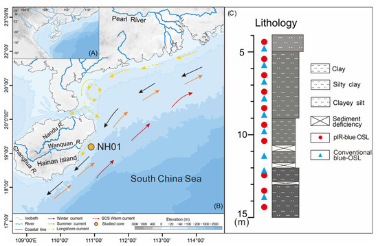
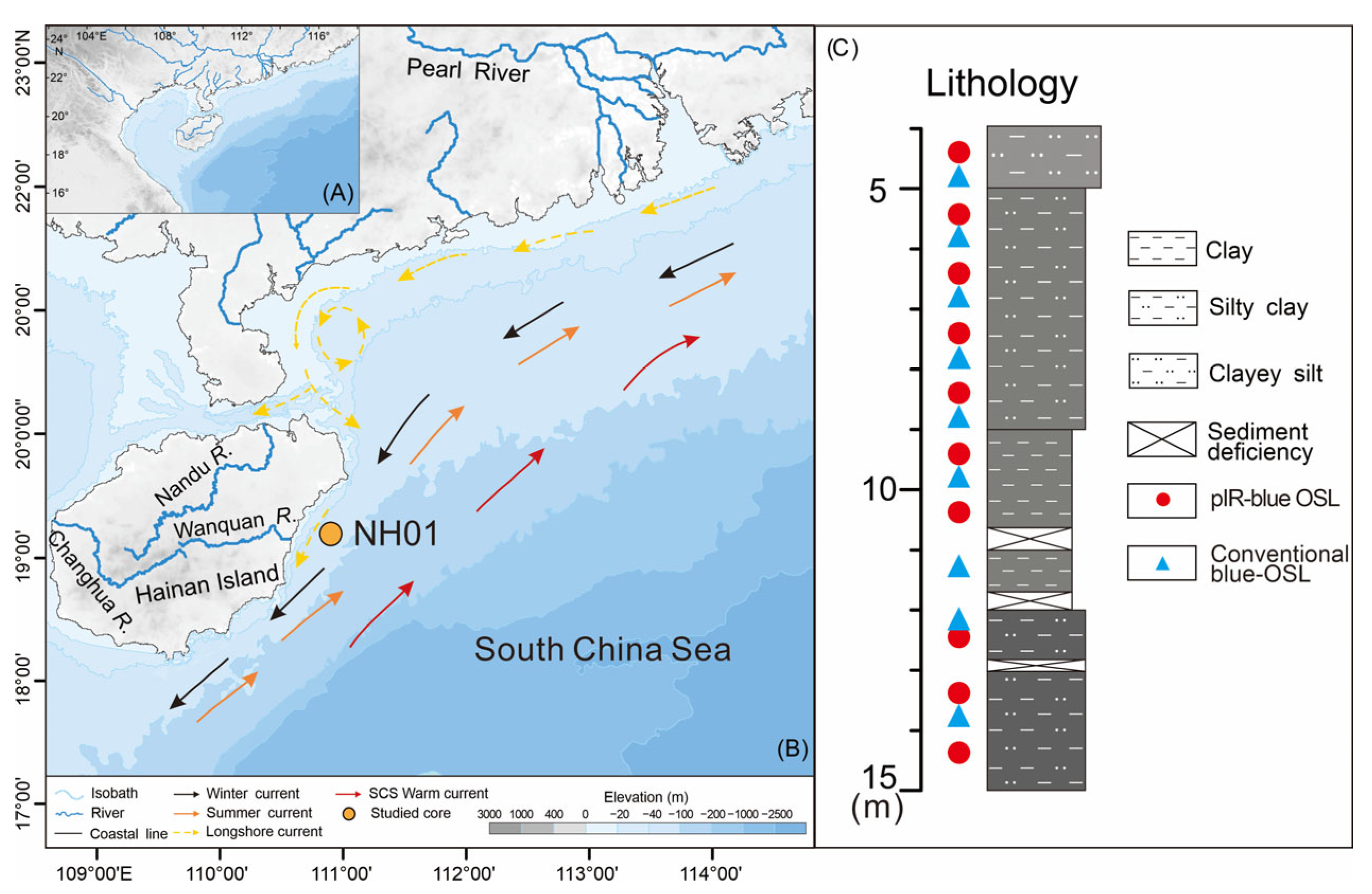
Figure 1.
(A,B) Study area and drilling site of core NH01. (C) Lithology characteristics, locations of the OSL samples core NH01 presented in this study, and those measured using the pIR-blue OSL protocol according to [17].
In the recently published work [17], the chronology of the core sediments from the East Hainan Coast, the inner shelf of the SCS, was established for the last 20 ka using the post-infrared blue-light stimulated luminescence (pIR-blue OSL) dating approach. The chronology and yielded sedimentation rate showed episodic deposition. In particular, a rapid deposition phase occurred in the early Holocene (~11.5–8.7 ka) [17]. Although the controlling factors of sea-level rise, precipitation and the resumed SCS longshore current to the early-Holocene sedimentation in the SCS continental shelf have been investigated in previous studies [13,14,15,16], the mechanism of the early-Holocene rapid sediment deposition remained uncertain. This is mainly related to the precision of the chronology and the accuracy of environmental reconstruction. A reliable geochronological constraint was crucial for interpreting the sedimentary evolution of the SCS continental shelf [18]. Optically stimulated luminescence (OSL) dating has been widely applied to various sedimentary environments, including marine, aeolian and alluvial sediments [17,19,20]. In recent years, marine sediments in the SCS continental shelf have been dated by the quartz OSL dating method [17,20,21]. OSL dating has been relatively advantageous compared to other methods, as the quartz and feldspar grains from in situ deposited clastic sediments have been directly dated [22]. However, it was shown that the sand-size quartz grains in the core sediments on the East Hainan Coast were contaminated by feldspar even after Hydrofluoric Acid (HF) etching, for which the blue-light stimulated OSL signal could be underestimated [23]. The post-infrared blue-light stimulated OSL (pIR-blue OSL) signal was used to largely reduce the effect of feldspar contamination, which, however, still probably slightly underestimated the real age [24].
The paleoenvironmental change could be reconstructed by using various environmental proxies, which correspond to different driving factors [25,26]. Among them, intensity and/or concentration change in the geochemical elements are thought to be related to the variation in sedimentary processes, such as erosion, transportation, weathering and deposition [27,28,29]. It has also been used to distinguish the source of sediments [30], to reconstruct marine–terrestrial interaction [31] and to investigate climate change [32] in the SCS.
In this study, the sediments in core NH01 from the SCS constrained to the period of early-Holocene were used for OSL dating and chemical element analysis (Figure 1). The fine-grained quartz samples were dated to refine the chronology of the early-Holocene deposits, associated with the period of rapid sedimentation. The high-resolution XRF scanning data (the intensities of Ti), with an interval of ~2.5 cm for the studied sequence, were interpreted. The objectives of this study are as follows: First, we aimed to compare the results of the conventional blue-OSL and pIR-blue OSL dating and to evaluate the impact of feldspar contamination. Second, it was aimed to better constrain the timing of the early-Holocene sedimentation. Finally, we aimed to interpret the intensity variation in the representative element (Ti) to understand the driving factors of sedimentary evolution on the East Hainan Coast, the inner shelf of the SCS, during the early-Holocene rapid depositional period.
2. Study Area
Hainan Island is located in the northwestern inner shelf of the SCS. Affected by the East Asian Summer Monsoon (EASM), Hainan Island experiences the northeastern monsoon wind in winter and the southwestern monsoon wind in summer [33]. The sediments of the East Hainan Coast have mainly come from the terrestrial input from the Chinese mainland and Hainan Island. The rivers originating from Hainan Island provide ~0.45 Mt./a sediments into the coastal area. The Pearl River exports 80 Mt./a sediments into the northern SCS [34].
The East Hainan Coast has a broad shelf, within the water depth of 100 m [35,36]. The sea surface temperature (SST) of the East Hainan Coast is 22.0–24.5 °C in winter and 27.4–31.0 °C in summer, respectively [37]. The seawater of the East Hainan Coast is controlled by the Guangdong Coastal Current (GCC), upwelling and SCS warm current. The GCC flows southwestward in winter and turns northeastward in summer affected by the EASM [33]. Upwelling is driven by the strong southwesterly summer monsoon and the topography [38]. A northeastward warm current exists in the shelf area [39]. In addition, a longshore current in the northern SCS is affected by the Pearl River runoff [17,40].
3. Samples and Methods
3.1. Materials and Samples
Core NH01
One sediment core, NH01, collected from the East Hainan Coast (19°15′ N, 110°57′ E, elevation: 73.5 m below sea-level) was analyzed (Figure 1). Sediments in the upper 13.80–4.80 m of the core were used for investigations of sedimentology and chronology in this study. The lithology of the core NH01 is shown in Figure 1C, which has been described and interpreted in detail in [17]. The sedimentary succession investigated in this study could be divided into three depositional units according to stratigraphic characteristics. The bottom unit (U3, 13.80–11.30 m) contains dark-gray silty clay. Shell debris was found in this unit, representing the depositional environment of marine–terrestrial interaction [17]. U2 (11.30–5.05 m) contains clay, silty clay and silty sand, with shell debris distributed at 8.80–8.70 m and 8.40–8.25 m, respectively [17]. The uppermost unit (U1, 5.05–4.80 m) consists of homogeneous gray silt, with shell debris distributed at 4.50–4.45 m and 1.45–1.43 m, respectively [17]. Both two upper units (U2 and U1) were likely formed under a neritic environment.
3.2. Luminescence Dating
3.2.1. Sample Preparation
All the luminescence samples were collected and dated under dim red light in the luminescence dating laboratory at China University of Geosciences Beijing (CUGB). Thirteen samples were collected from a depth interval of 15.40–4.80 m in the core NH01 in this study, and the results of eleven samples presented in the previous study were included for age comparison [17]. Fine-grained (FG, 4–11 μm) fractions were extracted for luminescence dating in this study. The outer 2 cm materials, which were potentially exposed to daylight, were used to measure the concentrations of uranium, thorium and potassium. The inner materials were treated with diluted 10% hydrochloric acid and 30% hydrogen peroxide to remove carbonates and organic matter, respectively. The FG fractions were settling according to Stokes’ law, and quartz grains were further extracted by fluorosilicic acid etching. The FG quartz grains were settled on aluminum aliquots using deionized water for equivalent dose (De) measurements.
3.2.2. Instrumentation and Methodology
Luminescence measurements were conducted using the automated Risø TL/OSL systems (DA-20) equipped with the 90Y/90Sr beta source, and the dose rate for FG quartz measurement was 0.09 Gy/s. The quartz OSL signal was stimulated by blue light-emitting diodes (LEDs, 470 ± 30 nm) and detected through a 7.5 mm Hoya U-340 filter. The conventional blue-OSL protocol was used for the De measurement in this study (Table 1). The conventional blue-OSL signal was calculated by subtracting the early background of 0.8–1.92 s from the first 0.8 s [41].

Table 1.
Single-aliquot regenerative-dose protocol for De measurements of quartz samples.
3.3. Dosimetry
The concentrations of uranium (ppm), thorium (ppm) and potassium (%) in the samples were measured by Inductively Coupled Plasma–Mass Spectrometry (ICP-MS) after drying and grinding. Based on the measured water contents and potential variation throughout geological history, the water content for all the samples was assumed to be 35 ± 5% [17]. Conversion factors [42] and beta attenuation [43] were used to calculate the external beta- and gamma-dose rates, respectively. A mean a-value of 0.04 ± 0.02 was applied for the dose rate calculation of the FG quartz [44]. In addition, the cosmic dose rate for each sample was calculated based on depth, altitude and geomagnetic latitude [45]. The dose rates for all samples are shown in Table 2.
Table 2.
Results of luminescence dating, including concentrations of U, Th and K, quartz environmental dose rate, De and ages.
3.4. X-Ray Fluorescence (XRF) Scanning
A total of 462 samples were collected from the core NH01 with an interval of 2.5 cm for X-ray fluorescence scanning using an XL2500 handheld XRF fluorescence spectrometer in the State Key Laboratory of Marine Geology of Tongji University. Titanium (Ti) has been widely used as a proxy for terrestrial input due to its geochemical stability and source-specific behavior [32,46]. In this study, the determined titanium intensity was used for paleoenvironmental reconstruction.
4. Results and Discussion
4.1. Revised Luminescence Chronology
4.1.1. Quartz Luminescence Characteristics and De Determination
According to [17], the preheat temperature was set to 200 °C for the De measurement of all samples. The De of FG quartz was measured using four aliquots. The decay curve and dose–response curve for the representative sample DS0354 are shown in Figure 2. The dose–response curves were fitted using the single saturating exponential function. The natural intensity was projected onto the dose–response curves to determine the De value for each aliquot. For those aliquots with an acceptable recycling ratio (0.9–1.1) and small recuperation (<5%), the De values were utilized for age determination. The standard error of the De value was calculated to present the De uncertainty in each sample. The range of the mean De values ranges from 29.79 ± 1.43 Gy to 39.16 ± 1.21 Gy. The quartz ages, calculated by dividing the mean De value by the environmental dose rate, range from 9.27 ± 0.56 ka to 12.18 ± 0.83 ka.
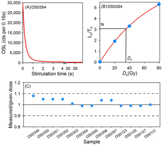
Figure 2.
Results of quartz OSL measurements, including decay curves of the natural OSL signals (A) and associated dose–response curve for the sample DS0354 (B). Dose recovery ratios for all samples are shown in (C).
4.1.2. Luminescence Ages and Sedimentation Rate
To assess the reliability of the preheat temperature applied in the single-aliquot regenerative dose (SAR) protocol, the dose recovery test was conducted for all samples. Three aliquots for each sample were first bleached and given a dose close to the De value. These aliquots were measured using the same SAR protocol as that for De determination. As shown in Figure 2C, the dose recovery ratios (measured dose/given dose) of all samples were within the range of 0.9–1.1, indicating that the preheat temperature was suitable for all samples.
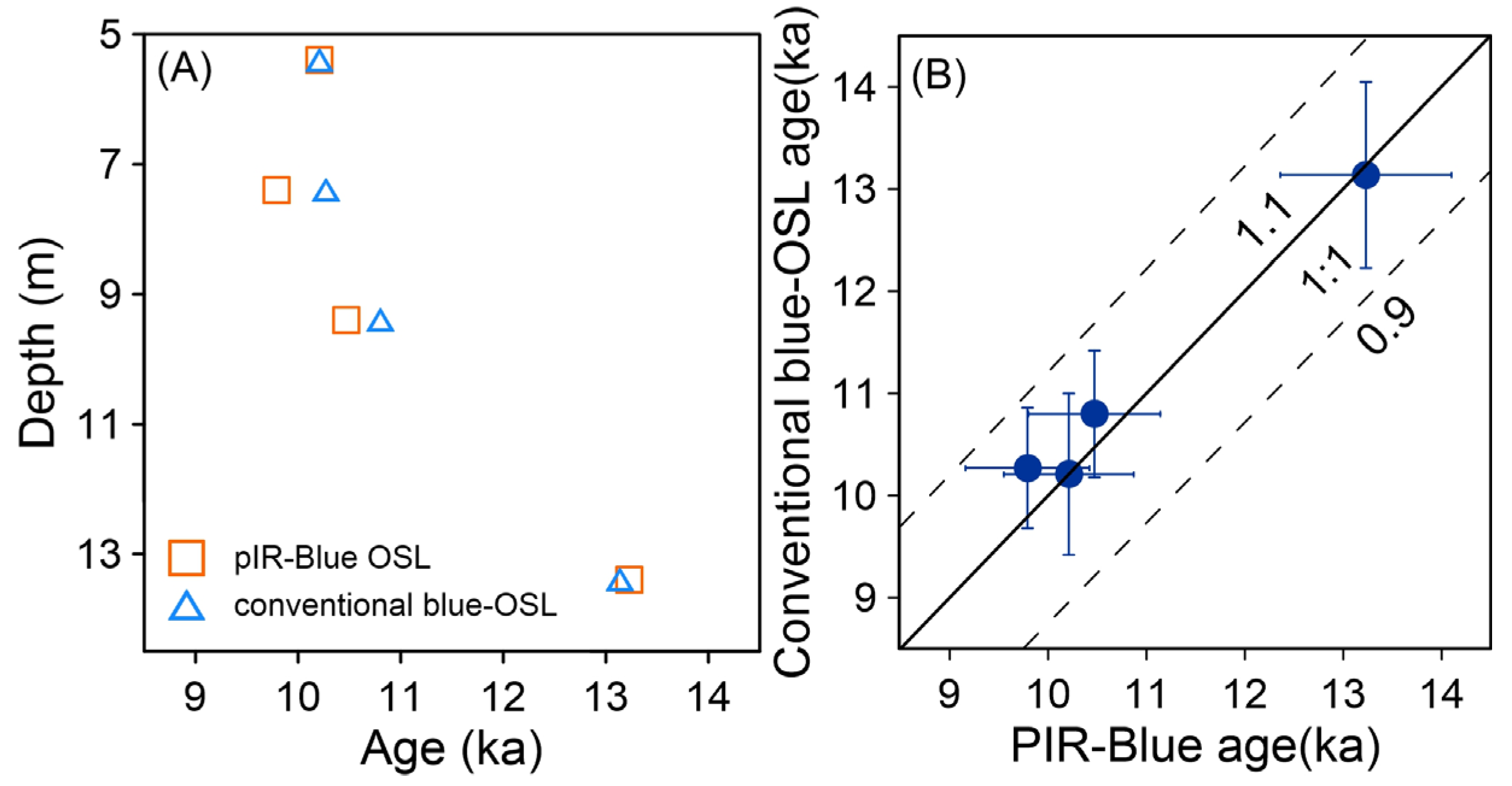
One potential problem in quartz OSL dating is contamination of the feldspar signals, which could lead to the underestimation of age [23]. This has been found in OSL dating using the sand-size quartz extracted from the core NH01, which was the main reason that the samples were dated using the pIR-blue OSL protocol [17]. However, the initial IR stimulation likely resulted in the signal loss of the lateral blue-light stimulated luminescence signal, and thus age underestimation, as concluded using raw sediments in [24]. Age comparison was carried out using four representative samples to evaluate the reliability of both the pIR-blue OSL and the conventional OSL results. As shown in Figure 3, the conventional blue-OSL ages agree with the corresponding pIR-blue OSL ages, suggesting that the initial IR stimulation did not affect the lateral blue-light stimulated OSL signal for the fine-grained quartz samples. All the ages presented both in this study and in [17] were used to establish the chronological framework.
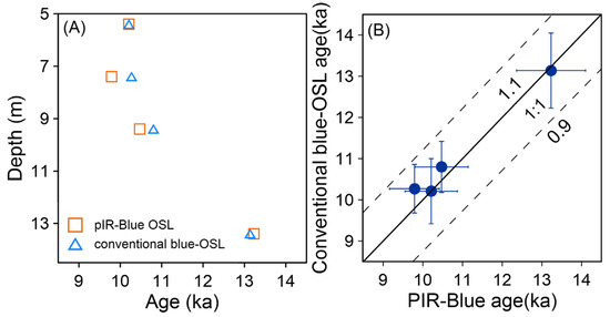
Figure 3.
Age comparisons between the conventional blue-OSL and pIR-blue OSL ages in lithological order (A) and in age-comparison plot (B).
The ‘Bacon’ age–depth model [47] was employed to establish the age–depth relationship for the section in the depth interval of 3.4–14.4 m in the core NH01. The age–depth model result drawn in Figure 4 shows that the refined chronology was more precise with relatively low-level uncertainty. The black line in Figure 4B showed the ratio of the refined median modeled ages over the previously published one [17], which tended towards 1.0. However, the modeled age uncertainty ratio (green line) of the refined one over the published one was generally lower than 1.0, especially for the time span of the early Holocene, suggesting that precision of the refined chronology was generally improved. According to the refined chronology, the sedimentation rate varied overall between 0.60 m/ka and 5.89 m/ka. The sedimentation rate was ~0.60 m/ka during 15.96–10.97 ka, which was higher than that in the period before the onset of the last deglaciation (19.70–15.96 ka) [17]. The sedimentation rate continued to rise to 5.89 m/ka during 10.97–9.27 ka.
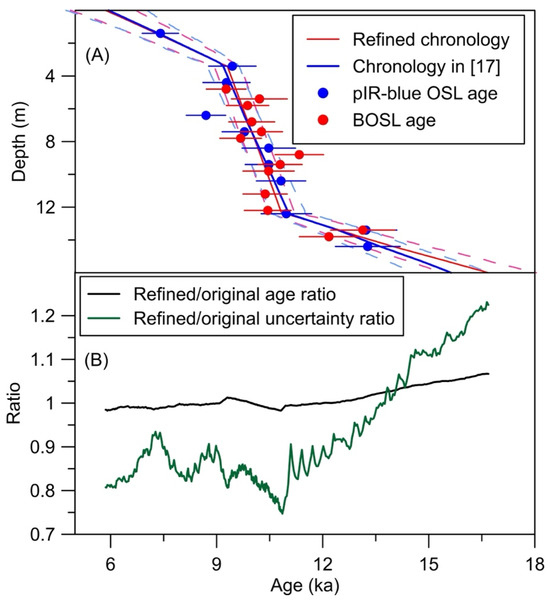
Figure 4.
Refined age–depth model and age comparison. (A) The refined OSL chronology was established using both the conventional blue-light stimulated OSL (BOSL, this study) and the pIR-blue OSL ages [17]. The dotted lines showed 95% intervals of uncertainty. (B) The refined modeled age and the associated age uncertainty were compared with those based on the pIR-blue OSL chronology [17] using the age and age uncertainty ratios, respectively.
4.2. Titanium Intensities, Flux and Environmental Implications
Significant climate change occurred during the Younger Dryas (YD) period and early Holocene [48,49,50]. The YD event was considered a millennium-scale extreme cooling event, interrupting the warming trend during the last deglaciation [51]. The rates of global sea-level rise consequently varied, but the sea level exhibited a generally rising trend [52]. Both climate warming and sea-level rise resulted in significant flux variation and geomorphological evolution in the northern continental shelf during the early Holocene [35,53,54,55,56]. The characteristics of rapid sedimentation during the early Holocene revealed in the core NH01 fortunately were ideal for investigating the details of sedimentary transportation and its driving factors [17]. Titanium as an indicator of terrigenous input was used in this study [46,57,58,59,60]. Apart from Ti intensity, the value of Ti accumulation was calculated by multiplying the intensity with the associated sedimentation rate determined by the Bacon age–depth model (Figure 4). It could be used to quantify the terrigenous (land-derived) material delivered to marine or lacustrine systems over time on the East Hainan Coast, reflecting both the Ti intensity and transport dynamics. In particular, the Ti flux represented the accumulation rate of Ti-bearing minerals (e.g., ilmenite, rutile) from continental weathering.
4.2.1. Ti Intensity and Flux Variation During ~16.0–7.0 ka
The Ti intensity results of the core NH01 are shown in Figure 5A. The range of variation for Ti element intensity was 1.04–4.21 × 10³, with an average value of 2.96 × 10³. From 16.0 to 14.2 ka, the Ti intensity showed a rapid increase trend. During 14.2–12.8 ka, the intensity first decreased and then increased. From 12.8 to 9.8 ka, the intensity of Ti was maintained at a relatively high level, and extremely high intensity was found at 10.5 and 9.8 ka, respectively. Then, the Ti element intensity began to decrease. Figure 5D shows the flux variation in the Ti element, which could be divided into three stages. The flux variation fluctuated slowly during the periods at 16.0–11.0 ka and 9.3–7.0 ka, while it increased extremely rapidly at 11.0 ka and remained high during 11.0–9.3 ka. Two distinct peaks of Ti flux were observed during the period of rapid change, centered at 10.5 and 9.8 ka, respectively. This interval of pronounced Ti flux variability exhibited remarkable synchronicity with the accelerated sedimentation rates recorded in the core NH01.
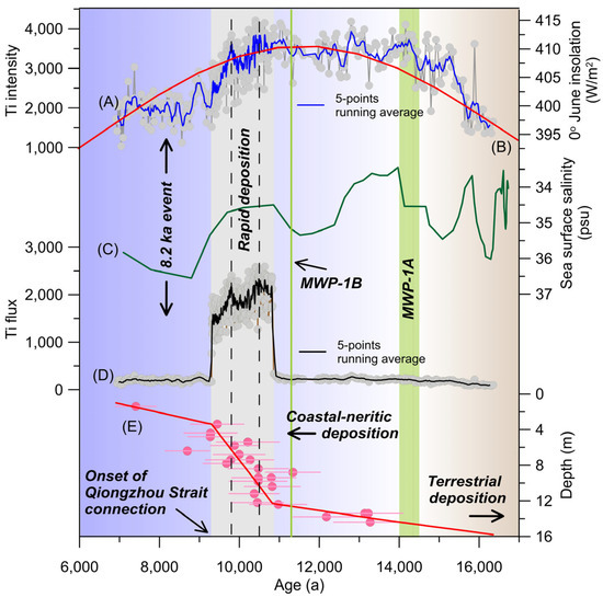
Figure 5.
The refined OSL chronology-based titanium intensity and flux variations and environmental correlations. (A) The titanium variation. The gray line with dot shows the measured Ti intensity. The blue line demonstrates Ti intensity variation with 5-points running average. (B) The red line shows the reconstructed solar insolation in tropical areas in June [61,62]. (C) The reconstructed sea surface salinity (SSS) curve is in green [63]. (D) The curve of titanium flux variation during ~16.0–7.0 ka according to titanium intensity and the sedimentation rate, for which the original data are shown in gray and the 5-points running average curve is in black. (E) The refined OSL chronology is demonstrated as the absolute ages by luminescence approach (pink dots) and the modelled age-depth relationship (pink line). The gradient blue and brown bars represent the coastal-neritic and terrestrial deposition during 7.0–14.3 ka and 14.3–17.0 ka, respectively. The green bars show the meltwater pulse 1A (~11.3 ka) and 1B (14.5–14.0 ka) events, respectively. The light-gray bar demonstrates the rapid depositional period according to the chronological framework.
4.2.2. Environmental Evolution on the East Hainan Coast During ~16.0–7.0 ka by the Refined OSL Chronology and Titanium Characteristics
During the period of approximately 16.0–11.0 ka, the global temperature gradually increased but remained relatively low. As glaciers gradually receded, sea levels began to rise from the low stand of −120 m [52], which rose to −55 m at 11.0 ka. Particularly, global warming during the Bølling–Allerød episode (ca. 14.7–12.9 ka) warming event caused the polar glacier meltwater to enter the global oceans [64]. According to the previous study, the summer solar insolation (near the equator) increased during 17.0 to 11.3 ka and then decreased from 11.3 to 6.0 ka (Figure 5B). It was consistent with the trend of Ti intensity variation, indicating the strengthening of the EASM during the last deglaciation [10]. Global warming in conjunction with polar glaciers melting resulted in two major meltwater pulse (MWP) events. Under the influence of MWP-1A, the sea level rose rapidly during 14.5–14.0 ka [64].
The sequences of sea surface salinity (SSS) in the northern SCS were reconstructed in [63]. As shown in Figure 5, the SSS rapidly decreased after MWP-1A. However, there was no significant decrease in the SSS after the occurrence of MWP-1B. A favorable correspondence still existed between MWP-1A and the SSS change curve under the possible hysteresis of salinity changes. On the contrary, the Ti flux showed a significant response to MWP-1B, showing a rapid increase trend after it, but was not sensitive to MWP-1A (Figure 5). The main cause of this phenomenon is likely due to differences in the input of terrestrial sediments. The strengthening of the EASM and the northward migration of the Intertropical Convergence Zone (ITCZ) occurred during the early Holocene, especially during MWP-1B [65,66,67,68,69,70]. Under the joint influence of both, the tropical atmospheric circulation and hydrological conditions brought abundant precipitation and a large amount of material deposition to the study area [66]. Terrestrial-derived sediments were transported to the coastal-neritic areas by runoff during the period of abundant precipitation, and subsequently further carried away by the coastal currents [71,72,73]. As a result, the Ti flux rapidly increased in the study area after MWP-1B, which was not observed after MWP-1A. Two abrupt increase points in Ti flux could be identified during the rapid deposition stage of 10.97–9.27 ka, namely at 10.5 and 9.8 ka, which might be due to the sudden strengthening of the monsoon. In addition, less vegetation coverage might also result in a high Ti flux, and the scarcity of vegetation exacerbates soil erosion, leading to an increase in terrestrial sediments. The pollen scarcity was observed in previous studies during the early Holocene [56]. However, the pollen concentration could have been diluted by the rapid sedimentation, resulting in difficulty in proving the impact of land cover.
The Ti flux significantly decreased after 9.27 ka (Figure 5), which might be attributed to several factors. Firstly, the continuously rising sea level connected the Qiongzhou Strait, which began to be invaded by seawater at around 10.0 ka and was fully submerged at around 8.5 ka [53,54], and then changed the geomorphology, sedimentary environment and ocean circulation patterns [74]. The increased water depth in the study area resisted the access of terrestrial sediments [52]. It also resulted in the changing of sediment transportation in the northern SCS [75]. For instance, sediments from the Pearl River could be carried and deposited into the Beibu Gulf, while most of these sediments had accumulated along the eastern of the Hainan Island before the Qiongzhou Strait was inundated [17]. Moreover, the decrease in Ti flux might be related to the weakening of monsoons caused by the 8.2 ka event. The weakened EASM has reduced precipitation and diminished terrestrial-derived sediments, which were transported to the coastal-neritic areas during the period of abrupt climate change [76].
5. Conclusions
This study established a high-resolution chronology of sedimentary sequences in the neritic area of the east coast of Hainan. A comparison of the pIR-blue OSL signal with the conventional blue-OSL signal was conducted in this study. We reconstructed the sedimentary evolution of the SCS continental shelf during the transformation from the YD period to the early Holocene using environmental proxy indicators. We draw our conclusions as follows:
- Both the pIR-blue OSL and conventional blue-OSL signal are applicable in this study. The feldspar contamination was almost negligible for the fine-grained quartz fraction.
- According to the refined chronology, two sedimentation stages were divided from the YD period to the early Holocene. The sedimentation rate was ca. 0.60 m/ka before 10.97 ka, while it increased abruptly (ca. 5.89 m/ka) during the period of 10.97–9.27 ka.
- During 16.00–9.27 ka, the evolution of both EASM and MWP events was driving the sedimentary process. MWP-1B triggered a surge in Ti flux at 10.5 and 9.8 ka due to the intensified monsoon-driven runoff and ITCZ-driven precipitation. In contrast, the Ti flux was not sensitive to MWP-1A due to the lack of input from terrestrial sediments. The sea-level rise (the connection of Qiongzhou Strait, ~8.5 ka) reconstructed the coastal geomorphology, diverting sediment transport pathways and isolating the study area from terrigenous inputs.
Author Contributions
Conceptualization and methodology, Y.L. (Yan Li), Y.X. and X.S.; formal analysis, M.C., Y.L. (Yang Li), W.L. and X.W.; original draft preparation, M.C., X.S., Y.L. (Yang Li) and Y.L. (Yan Li); review and editing, X.S., Y.X. and Y.L. (Yan Li). All authors have read and agreed to the published version of the manuscript.
Funding
This research was supported by the Hainan Provincial Joint Project of Sanya Yazhou Bay Science and Technology City, Grant (No. 2021JJLH0076), the Hainan Provincial Department of Finance Special Project of ‘Investigation and Evaluation of the Solid Mineral Resource Potentials in the South China Sea’ (No. T100732), the 111 Project (No. B20011) and the Shandong Provincial Natural Science Foundation (ZR2023QD154).
Institutional Review Board Statement
Not applicable.
Informed Consent Statement
Not applicable.
Data Availability Statement
Data are available on request the corresponding author (xiaosun@cugb.edu.cn).
Acknowledgments
We appreciate Wenjing Liu and Yibing Li for laboratory assistance.
Conflicts of Interest
The authors declare no conflicts of interest.
References
- Moros, M.; Andrews, J.T.; Eberl, D.D.; Jansen, E. Holocene history of drift ice in the northern North Atlantic: Evidence for different spatial and temporal modes. Paleoceanography 2006, 21. [Google Scholar] [CrossRef]
- Tan, L.; Xu, H. Editorial: Holocene Climate Changes in the Asia Pacific Region. Front. Earth Sci. 2021, 8, 622792. [Google Scholar] [CrossRef]
- Hong, Y.T.; Hong, B.; Lin, Q.A.; Shibata, Y.; Hirota, M.; Zhu, Y.X.; Leng, X.T.; Wang, T.; Yi, L. Inverse phase oscillations between the East Asian and Indian Ocean summer monsoons during the last 12,000 years and paleo-El Niño. Earth Planet. Sci. Lett. 2005, 231, 337–346. [Google Scholar] [CrossRef]
- Rasmussen, S.O.; Vinther, B.M.; Clausen, H.B.; Andersen, K.K. Early Holocene climate oscillations recorded in three Greenland ice cores. Quat. Sci. Rev. 2007, 26, 1907–1914. [Google Scholar] [CrossRef]
- Yao, S.; Ling, C.; Lu, H.; Meng, Y.; Li, C.; Yu, S.Y.; Xue, B.; Wang, G. Palynological and sedimentological evidence for early mid-Holocene hydroclimatic variability in the Ningshao Plain, East China. Palaeogeogr. Palaeoclimatol. Palaeoecol. 2024, 637, 111997. [Google Scholar] [CrossRef]
- Choi, S.J.; Merritts, D.J.; Ota, Y. Elevations and ages of marine terraces and late Quaternary rock uplift in southeastern Korea. J. Geophys. Res. Solid Earth 2008, 113. [Google Scholar] [CrossRef]
- Liu, J.; Zhang, X.; Mei, X.; Zhao, Q.; Guo, X.; Zhao, W.; Liu, J.; Saito, Y.; Wu, Z.; Li, J.; et al. The sedimentary succession of the last~ 3.50 Myr in the western South Yellow Sea: Paleoenvironmental and tectonic implications. Mar. Geol. 2018, 399, 47–65. [Google Scholar] [CrossRef]
- Yin, A.; Harrison, T.M. Geologic evolution of the Himalayan-Tibetan orogen. Annu. Rev. Earth Planet. Sci. 2000, 28, 211–280. [Google Scholar] [CrossRef]
- Liu, W.T.; Xie, X. Spacebased observations of the seasonal changes of South Asian monsoons and oceanic responses. Geophys. Res. Lett. 1999, 26, 1473–1476. [Google Scholar] [CrossRef]
- Shintani, T.; Yamamoto, M.; Chen, M.T. Paleoenvironmental changes in the northern South China Sea over the past 28,000 years: A study of TEX86-derived sea surface temperatures and terrestrial biomarkers. J. Asian Earth Sci. 2011, 40, 1221–1229. [Google Scholar] [CrossRef]
- Ge, Q.; Liu, J.P.; Xue, Z.; Chu, F. Dispersal of the Zhujiang River (Pearl River) derived sediment in the Holocene. Acta Oceanol. Sin. 2014, 33, 1–9. [Google Scholar] [CrossRef]
- Li, M.; Ouyang, T.; Tian, C.; Zhu, Z.; Peng, S.; Tang, Z.; Qiu, Z.; Zhong, H.; Peng, X. Sedimentary responses to the East Asian monsoon and sea level variations recorded in the northern South China Sea over the past 36 kyr. J. Asian Earth Sci. 2019, 171, 213–224. [Google Scholar] [CrossRef]
- Zhou, L.; Yang, Y.; Wang, Z.; Jia, J.; Mao, L.; Li, Z.; Fang, X.; Gao, S. Investigating ENSO and WPWP modulated typhoon variability in the South China Sea during the mid–late Holocene using sedimentological evidence from southeastern Hainan Island, China. Mar. Geol. 2019, 416, 105987. [Google Scholar] [CrossRef]
- Cao, L.; Liu, J.; Shi, X.; He, W.; Chen, Z. Source-to-sink processes of fluvial sediments in the northern South China Sea: Constraints from river sediments in the coastal region of South China. J. Asian Earth Sci. 2019, 185, 104020. [Google Scholar] [CrossRef]
- Zong, Y.; Huang, K.; Yu, F.; Zheng, Z.; Switzer, A.; Huang, G.; Wang, N.; Tang, M. The role of sea-level rise, monsoonal discharge and the palaeo-landscape in the early Holocene evolution of the Pearl River delta, southern China. Quat. Sci. Rev. 2012, 54, 77–88. [Google Scholar] [CrossRef]
- Bradley, S.L.; Milne, G.A.; Horton, B.P.; Zong, Y. Modelling Sea level data from China and Malay-Thailand to estimate Holocene ice-volume equivalent sea level change. Quat. Sci. Rev. 2016, 137, 54–68. [Google Scholar] [CrossRef]
- Li, Y.; Li, Y.; Chen, M.; Xue, Y.; Zhang, J.; Wang, L.; Tong, C.; Yi, L. Sediment flux variation and environmental implications in the East Hainan Coast, South China Sea during the last 20 ka—A luminescence chronological investigation. Mar. Geol. 2025, 480, 107453. [Google Scholar] [CrossRef]
- Kaufman, D.; McKay, N.; Routson, C.; Erb, M.; Davis, B.; Heiri, O.; Jaccard, S.; Tierney, J.; Datwyler, C.; Axford, Y.; et al. A global database of Holocene paleotemperature records. Sci. Data 2020, 7, 1–34. [Google Scholar] [CrossRef]
- Fuchs, M.; Owen, L.A. Luminescence dating of glacial and associated sediments: Review, recommendations and future directions. Boreas 2008, 37, 636–659. [Google Scholar] [CrossRef]
- Zhong, J.; Ling, K.; Yang, M.; Shen, Q.; Abbas, M.; Lai, Z. Radiocarbon and OSL dating on cores from the Chaoshan delta in the coastal South China Sea. Front. Mar. Sci. 2022, 9, 1030841. [Google Scholar] [CrossRef]
- Jiang, T.; Liu, X.; Yu, T.; Hu, Y. OSL dating of late Holocene coastal sediments and its implication for sea-level eustacy in Hainan Island, Southern China. Quat. Int. 2018, 468, 24–32. [Google Scholar] [CrossRef]
- Preusser, F.; Degering, D.; Fuchs, M.; Hilgers, A.; Kadereit, A.; Klasen, N.; Krbetschek, M.; Richter, D.; Spencer, J.Q. Luminescence dating: Basics, methods and applications. EG Quat. Sci. J. 2008, 57, 95–149. [Google Scholar] [CrossRef]
- Wintle, A.G.; Murray, A.S. A review of quartz optically stimulated luminescence characteristics and their relevance in single-aliquot regeneration dating protocols. Radiat. Meas. 2006, 41, 369–391. [Google Scholar] [CrossRef]
- Roberts, H.M.; Wintle, A.G. Luminescence sensitivity changes of polymineral fine grains during IRSL and [post-IR] OSL measurements. Radiat. Meas. 2003, 37, 661–671. [Google Scholar] [CrossRef]
- Wang, L.; Hu, S.; Yu, G.; Ma, M.; Wang, Q.; Zhang, Z.; Liao, M.; Gao, L.; Ye, L.; Wang, X. Magnetic characteristics of sediments from a radial sand ridge field in the South Yellow Sea, eastern China, and environmental implications during the mid-to late-Holocene. J. Asian Earth Sci. 2018, 163, 224–234. [Google Scholar] [CrossRef]
- Shilling, A.M.; Colcord, D.E.; Karty, J.; Hansen, A.; Freeman, K.H.; Njau, J.K.; Stanistreet, I.G.; Stollhofen, H.; Schich, K.D.; Toth, N.; et al. Biogeochemical evidence from OGCP Core 2A sediments for environmental changes preceding deposition of Tuff IB and climatic transitions in Upper Bed I of the Olduvai Basin. Palaeogeogr. Palaeoclimatol. Palaeoecol. 2020, 555, 109824. [Google Scholar] [CrossRef]
- Hussain, A.; Al-Ramadan, K. A core-based XRF scanning workflow for continuous measurement of mineralogical variations in clastic reservoirs. MethodsX 2022, 9, 101928. [Google Scholar] [CrossRef] [PubMed]
- Almenningen, S.; Roy, S.; Hussain, A.; Seland, J.G.; Ersland, G. Effect of mineral composition on transverse relaxation time distributions and MR imaging of tight rocks from offshore Ireland. Minerals 2020, 10, 232. [Google Scholar] [CrossRef]
- Hussain, A.; Haughton, P.D.; Shannon, P.M.; Turner, J.N.; Pierce, C.S.; Obradors-Latre, A.; Barker, S.P.; Martinsen, O.J. High-resolution X-ray fluorescence profiling of hybrid event beds: Implications for sediment gravity flow behaviour and deposit structure. Sedimentology 2020, 67, 2850–2882. [Google Scholar] [CrossRef]
- Li, T.; Li, X.; Zhang, J.; Luo, W.; Tian, C.; Zhao, L. Source identification and co-occurrence patterns of major elements in South China Sea sediments. Mar. Geol. 2020, 428, 106285. [Google Scholar] [CrossRef]
- Sun, Y.; Wu, F.; Clemens, S.C.; Oppo, D.W. Processes controlling the geochemical composition of the South China Sea sediments during the last climatic cycle. Chem. Geol. 2008, 257, 240–246. [Google Scholar] [CrossRef]
- Xie, J.; Zhao, B.; Zhan, Q.; Li, X. Review of geochemical applications for paleoenvironmental and paleoecological analyses. Shanghai Land Resour. 2015, 3, 64–70, (In Chinese with English Abstract). [Google Scholar]
- Zhang, J.; Wang, D.R.; Jennerjahn, T.; Dsikowitzky, L. Land–sea interactions at the east coast of Hainan Island, South China Sea: A synthesis. Cont. Shelf Res. 2013, 57, 132–142. [Google Scholar] [CrossRef]
- Liu, Z.; Tuo, S.; Colin, C.; Liu, J.T.; Huang, C.Y.; Selvaraj, K.; Chen, C.T.; Zhao, Y.; Siringan, F.P.; Boulay, S.; et al. Detrital fine-grained sediment contribution from Taiwan to the northern South China Sea and its relation to regional ocean circulation. Mar. Geol. 2008, 255, 149–155. [Google Scholar] [CrossRef]
- Xu, F.; Hu, B.; Dou, Y.; Liu, X.; Wan, S.; Xu, Z.; Tian, X.; Liu, Z.; Li, A. Sediment provenance and paleoenvironmental changes in the northwestern shelf mud area of the South China Sea since the mid-Holocene. Cont. Shelf Res. 2017, 144, 21–30. [Google Scholar] [CrossRef]
- Chen, Y.; Deng, B.; Chen, Y.; Wang, D.; Zhang, J. Holocene sedimentary evolution of a subaqueous delta off a typical tropical river, Hainan Island, South China. Mar. Geol. 2021, 442, 106664. [Google Scholar] [CrossRef]
- Locarnini, R.A.; Mishonov, A.V.; Baranova, O.K.; Boyer, T.P.; Zweng, M.M.; Garcia, H.E.; Reagan, J.R.; Seidov, D.; Weathers, K.W.; Paver, C.R.; et al. World Ocean Atlas 2018, Volume 1: Temperature. In NOAA Atlas NESDIS, 81; Mishonov, A., Ed.; National Centers for Environmental Information: Silver Spring, MD, USA, 2019; p. 52. [Google Scholar]
- Jing, Z.Y.; Qi, Y.Q.; Hua, Z.L.; Zhang, H. Numerical study on the summer upwelling system in the northern continental shelf of the South China Sea. Cont. Shelf Res. 2009, 29, 467–478. [Google Scholar] [CrossRef]
- Yin, J.; Huang, L.; Li, K.; Lian, S.; Li, C.; Lin, Q. Abundance distribution and seasonal variations of Calanus sinicus (Copepoda: Calanoida) in the northwest continental shelf of South China Sea. Cont. Shelf Res. 2011, 31, 1447–1456. [Google Scholar] [CrossRef]
- Li, K.Z.; Yin, J.Q.; Huang, L.M.; Lian, S.M.; Zhang, J.L.; Liu, C.G. Monsoon-forced distribution and assemblages of appendicularians in the northwestern coastal waters of South China Sea. Estuar. Coast. Shelf Sci. 2010, 89, 145–153. [Google Scholar] [CrossRef]
- Cunningham, A.C.; Wallinga, J. Selection of integration time intervals for quartz OSL decay curves. Quat. Geochronol. 2010, 5, 657–666. [Google Scholar] [CrossRef]
- Guérin, G.; Mercier, N.; Adamiec, G. Dose-rate conversion factors: Update. Anc. Tl 2011, 29, 5–8. [Google Scholar] [CrossRef]
- Mejdahl, V. Thermoluminescence dating: Beta-dose attenuation in quartz grains. Archaeometry 1979, 21, 61–72. [Google Scholar] [CrossRef]
- Rees-Jones, J. Optical dating of young sediments using fine-grain quartz. Anc. TL 1995, 13, 9–14. [Google Scholar] [CrossRef]
- Prescott, J.R.; Hutton, J.T. Cosmic ray contributions to dose rates for luminescence and ESR dating: Large depths and long-term time variations. Radiat. Meas. 1994, 23, 497–500. [Google Scholar] [CrossRef]
- Murray, R.W.; Leinen, M.; Isern, A. Biogenic flux of Al to sediment in the central equatorial Pacific Ocean: Evidence for increased productivity during glacial periods. Paleoceanography 1993, 8, 651–670. [Google Scholar] [CrossRef]
- Blaauw, M.; Christen, J.A. Flexible paleoclimate age-depth models using an autoregressive gamma process. Bayesian Anal. 2011, 6, 457–474. [Google Scholar] [CrossRef]
- Fang, K.; Cai, B.; Liu, X.; Lei, G.; Jiang, X.; Zhao, Y.; Li, H.; Seppä, H. Climate of the late Pleistocene and early Holocene in coastal South China inferred from submerged wood samples. Quat. Int. 2017, 447, 111–117. [Google Scholar] [CrossRef]
- Kong, D.; Wei, G.; Chen, M.T.; Peng, S.; Liu, Z. Northern South China Sea SST changes over the last two millennia and possible linkage with solar irradiance. Quat. Int. 2017, 459, 29–34. [Google Scholar] [CrossRef]
- Yan, T.; Yu, K.; Jiang, L.; Li, Y.; Zhao, N. Significant sea-level fluctuations in the western tropical Pacific during the mid-Holocene. Paleoceanogr. Paleoclimatol. 2024, 39, e2023PA004783. [Google Scholar] [CrossRef]
- Chen, X.; Wu, D.; Huang, X.; Lv, F.; Brenner, M.; Jin, H.; Chen, F. Vegetation response in subtropical southwest China to rapid climate change during the Younger Dryas. Earth-Sci. Rev. 2020, 201, 103080. [Google Scholar] [CrossRef]
- Lambeck, K.; Rouby, H.; Purcell, A.; Sun, Y.; Sambridge, M. Sea level and global ice volumes from the Last Glacial Maximum to the Holocene. Proc. Natl. Acad. Sci. USA 2014, 111, 15296–15303. [Google Scholar] [CrossRef]
- Zhao, H.; Wang, L.; Yuan, J. Origin and time of Qiongzhou Strait. Mar. Geol. Quat. Geol. 2007, 27, 33–40. [Google Scholar]
- Shi, M.; Chen, C.; Xu, Q.; Lin, H.; Liu, G.; Wang, H.; Wang, F.; Yan, J. The role of Qiongzhou Strait in the seasonal variation of the South China Sea circulation. J. Phys. Oceanogr. 2002, 32, 103–121. [Google Scholar] [CrossRef]
- Xiong, H.; Zong, Y.; Qian, P.; Huang, G.; Fu, S. Holocene sea-level history of the northern coast of South China Sea. Quat. Sci. Rev. 2018, 194, 12–26. [Google Scholar] [CrossRef]
- Dodson, J.; Li, J.; Lu, F.; Zhang, W.; Yan, H.; Cao, S. A late pleistocene and holocene vegetation and environmental record from Shuangchi Maar, Hainan Province, South China. Palaeogeogr. Palaeoclimatol. Palaeoecol. 2019, 523, 89–96. [Google Scholar] [CrossRef]
- Goldberg, E.D.; Arrhenius, G.O.S. Chemistry of Pacific pelagic sediments. Geochim. Cosmochim. Acta 1958, 13, 153–212. [Google Scholar] [CrossRef]
- Schroeder, J.O.; Murray, R.W.; Leinen, M.; Pflaum, R.C.; Janecek, T.R. Barium in equatorial Pacific carbonate sediment: Terrigenous, oxide, and biogenic associations. Paleoceanography 1997, 12, 125–146. [Google Scholar] [CrossRef]
- Murray, R.W.; Knowlton, C.; Leinen, M.; Mix, A.C.; Polsky, C.H. Export production and carbonate dissolution in the central equatorial Pacific Ocean over the past 1 Myr. Paleoceanography 2000, 15, 570–592. [Google Scholar] [CrossRef]
- Wei, G.; Liu, Y.; Li, X.; Shao, L.; Liang, X. Climatic impact on Al, K, Sc and Ti in marine sediments: Evidence from ODP Site 1144, South China Sea. Geochem. J. 2003, 37, 593–602. [Google Scholar] [CrossRef]
- Cheng, H.; Edwards, R.L.; Sinha, A.; Spötl, C.; Yi, L.; Chen, S.; Kelly, M.; Kathayat, G.; Wang, X.; Li, X.; et al. The Asian monsoon over the past 640,000 years and ice age terminations. Nature 2016, 534, 640–646. [Google Scholar] [CrossRef]
- Berger, A. Long-term variations of caloric insolation resulting from the Earth’s orbital elements. Quat. Res. 1978, 9, 139–167. [Google Scholar] [CrossRef]
- Yin, J.; Yang, X.; Zhou, Q.; Li, G.; Gao, H.; Liu, J. Sea surface temperature and salinity variations from the end of Last Glacial Maximum (LGM) to the Holocene in the northern South China Sea. Palaeogeogr. Palaeoclimatol. Palaeoecol. 2021, 562, 110102. [Google Scholar] [CrossRef]
- Liu, J.P.; Milliman, J.D. Reconsidering melt-water pulses 1A and 1B: Global impacts of rapid sea-level rise. J. Ocean Univ. China 2004, 3, 183–190. [Google Scholar] [CrossRef]
- Berger, A.; Loutre, M.F. Insolation values for the climate of the last 10 million years. Quat. Sci. Rev. 1991, 10, 297–317. [Google Scholar] [CrossRef]
- Haug, G.H.; Hughen, K.A.; Sigman, D.M.; Peterson, L.C.; Rohl, U. Southward migration of the intertropical convergence zone through the Holocene. Science 2001, 293, 1304–1308. [Google Scholar] [CrossRef]
- Bard, E.; Hamelin, B.; Delanghe-Sabatier, D. Deglacial meltwater pulse 1B and Younger Dryas Sea levels revisited with boreholes at Tahiti. Science 2010, 327, 1235–1237. [Google Scholar] [CrossRef] [PubMed]
- Zhou, X.; Sun, L.; Zhan, T.; Huang, W.; Zhou, X.; Hao, Q.; Wang, Y.; He, X.; Zhao, C.; Zhang, J.; et al. Time-transgressive onset of the Holocene Optimum in the East Asian monsoon region. Earth Planet. Sci. Lett. 2016, 456, 39–46. [Google Scholar] [CrossRef]
- Griffiths, M.L.; Johnson, K.R.; Pausata, F.S.; White, J.C.; Henderson, G.M.; Wood, C.T.; Yang, H.; Ersek, V.; Conrad, C.; Sekhon, N. End of Green Sahara amplified mid-to late Holocene megadroughts in mainland Southeast Asia. Nat. Commun. 2020, 11, 4204. [Google Scholar] [CrossRef] [PubMed]
- Huang, X.; Zhang, H.; Griffiths, M.L.; Zhao, B.; Pausata, F.S.; Tabor, C.; Shu, J.; Xie, S. Holocene forcing of East Asian hydroclimate recorded in a subtropical peatland from southeastern China. Clim. Dyn. 2023, 60, 981–993. [Google Scholar] [CrossRef]
- Kuehl, S.A.; Levy, B.M.; Moore, W.S.; Allison, M.A. Subaqueous delta of the Ganges-Brahmaputra River system. Mar. Geol. 1997, 144, 81–96. [Google Scholar] [CrossRef]
- Xu, G.; Bi, S.; Gugliotta, M.; Liu, J.; Liu, J.P. Dispersal mechanism of fine-grained sediment in the modern mud belt of the East China Sea. Earth-Sci. Rev. 2023, 240, 104388. [Google Scholar] [CrossRef]
- Liu, J.; Steinke, S.; Vogt, C.; Mohtadi, M.; Pol-Holz, R.; Hebbeln, D. Temporal and spatial patterns of sediment deposition in the northern South China Sea over the last 50,000 years. Palaeogeogr. Palaeoclimatol. Palaeoecol. 2017, 465, 212–224. [Google Scholar] [CrossRef]
- Chen, L.; Zhang, Y.F.; Li, T.J.; Yang, W.F.; Chen, J. Sedimentary environment and its evolution of Qiongzhou Strait and nearby seas since last ten thousand years. Earth Sci. 2014, 39, 696–704. [Google Scholar]
- Li, J.; Gao, J.; Wang, Y.; Li, Y.; Bai, F.; Cees, L. Distribution and dispersal pattern of clay minerals in surface sediments, eastern Beibu Gulf, South China Sea. Acta Oceanol. Sin. 2012, 31, 78–87. [Google Scholar] [CrossRef]
- Zhang, X.; Zhang, H.; Zhang, R.; Wang, J.; Wang, M.; Liang, Z.; He, M.; Wei, R.; Cheng, H. Spatiotemporal pattern of the East Asian monsoon hydroclimate during the 8.2 ka event inferred from a new speleothem multi-proxy record from SE China. Quat. Sci. Rev. 2025, 349, 109141. [Google Scholar] [CrossRef]


Disclaimer/Publisher’s Note: The statements, opinions and data contained in all publications are solely those of the individual author(s) and contributor(s) and not of MDPI and/or the editor(s). MDPI and/or the editor(s) disclaim responsibility for any injury to people or property resulting from any ideas, methods, instructions or products referred to in the content. |
© 2025 by the authors. Licensee MDPI, Basel, Switzerland. This article is an open access article distributed under the terms and conditions of the Creative Commons Attribution (CC BY) license (https://creativecommons.org/licenses/by/4.0/).