Adaptive Temporal Reinforcement Learning for Mapping Complex Maritime Environmental State Spaces in Autonomous Ship Navigation

Abstract

The autonomous decision-making model for ship navigation requires extensive interaction and trial-and-error in real, complex environments to ensure optimal decision-making performance and efficiency across various scenarios. However, existing approaches still encounter significant challenges in addressing the temporal features of state space and tackling complex dynamic collision avoidance tasks, primarily due to factors such as environmental uncertainty, the high dimensionality of the state space, and limited decision robustness. This paper proposes an adaptive temporal decision-making model based on reinforcement learning, which utilizes Long Short-Term Memory (LSTM) networks to capture temporal features of the state space. The model integrates an enhanced Proximal Policy Optimization (PPO) algorithm for efficient policy iteration optimization. Additionally, a simulation training environment is constructed, incorporating multi-factor coupled physical properties and ship dynamics equations. The environment maps variables such as wind speed, current velocity, and wave height, along with dynamic ship parameters, while considering the International Regulations for Preventing Collisions at Sea (COLREGs) in training the autonomous navigation decision-making model. Experimental results demonstrate that, compared to other neural network-based reinforcement learning methods, the proposed model excels in environmental adaptability, collision avoidance success rate, navigation stability, and trajectory optimization. The model’s decision resilience and state-space mapping align with real-world navigation scenarios, significantly improving the autonomous decision-making capability of ships in dynamic sea conditions and providing critical support for the advancement of intelligent shipping.

1. Introduction

The digitalization and intelligence of the maritime transportation industry are steadily progressing, with Maritime Autonomous Surface Ships (MASS) at the forefront of modern shipping innovation, garnering global attention. MASS offers a significant advantage in enhancing the safety and efficiency of shipping operations, particularly by reducing human errors and optimizing navigation decisions. However, in complex maritime environments, MASS continues to face several challenges, especially in collision avoidance decision-making tasks under real-world conditions. Existing research often suffers from overly simplistic environmental designs and lacks sufficient algorithmic robustness, failing to address issues such as the long-tail effect. This paper tackles challenges such as environmental uncertainty, high-dimensional state space, and inadequate decision robustness that autonomous vessels encounter in complex maritime navigation. It proposes an adaptive temporal reinforcement learning method, utilizing a simulation environment that closely mirrors real-world maritime conditions. This method simulates ship dynamics equations and introduces an adaptive temporal decision-making model. It integrates dynamic ship parameters (e.g., position, velocity, heading), environmental factors (e.g., wind speed, current velocity, wave height), and the motion trajectories of other vessels, while ensuring adherence to the COLREGs to achieve safe and efficient autonomous navigation and collision avoidance decision-making.

The ship navigation decision-making model incorporates various methods, including rule-based systems, game theory, expert systems, fuzzy logic, model predictive control, and deep reinforcement learning. The rule-based approach, the most fundamental decision-making method, relies on established navigation rules and logical reasoning, and is widely used in autonomous collision avoidance decision-making for ships. Zhang, Ruolan, and others proposed a decision-making method that combines rule-based and neural network approaches. Their results demonstrate strong robustness and collision avoidance capabilities, and the method can be extended to incorporate various sensor data, thereby enhancing the feasibility of unmanned navigation [1]. Perera, Lokukaluge P., and others addressed the issue of Mamdani inference failure in fuzzy logic-based collision avoidance decision-making by introducing smooth transition areas, optimizing the size of transition zones, and proposing a multi-level decision-making scheme. They developed a fuzzy inference system (FIS) based on IF-THEN rules [2]. Koch, Paul proposed a rule set based on electronic charts to enhance collision avoidance decision-making for unmanned vessels navigating narrow channels and operating under separation traffic schemes, thus, improving both autonomous navigation and compliance [3]. While rule-based methods can address autonomous decision-making challenges for unmanned vessels in localized areas, their poor generalization ability and over-reliance on predefined rules limit their broader applicability.

Fuzzy logic, which emulates human-like reasoning to handle uncertainty, is widely applied in autonomous collision avoidance and decision support systems. Perera, L.P. proposed an intelligent decision-making system based on fuzzy logic. This study analyzed the collision avoidance relationship between the own vessel and the target ship, developed a fuzzy inference system, and implemented it on the MATLAB platform [4]. Wu, Bing introduced a fuzzy logic-based ship-bridge collision warning method that comprehensively integrates ship characteristics, bridge parameters, and environmental factors. The study assessed collision risk through fuzzy inference and validated its effectiveness in ensuring safe navigation in bridge areas [5]. Wu, Bing also proposed a fuzzy logic-based decision-making method for selecting navigation strategies under inland waterway separation traffic schemes, analyzing dynamic factors such as free navigation, following, and overtaking vessels [6]. Liu, Wenwen presented a fuzzy logic-based multi-sensor data fusion algorithm, combining AIS and radar data to improve target vessel detection accuracy and optimizing computational efficiency with Kalman filtering [7]. Shi, Ziqiang developed a fuzzy logic-based method for regional multi-ship collision risk assessment, considering factors such as crossing angles, navigation environment, DCPA, and TCPA, and calculating risk weights using the Analytic Hierarchy Process (AHP) [8]. Fuzzy logic provides intuitive and efficient decision-making mechanisms for simple and well-defined tasks and environments. However, it faces challenges in high-dimensional problems, leading to excessive computational costs in more complex tasks.

Expert systems utilize knowledge bases and inference mechanisms to simulate human expert decision-making processes, with applications in rule-based reasoning, fault diagnosis, and intelligent decision support. Hanninen assessed the impact of enhanced navigation support information services—based on expert knowledge—on the risks of ship collisions and groundings in the Gulf of Finland, analyzing the results using a Bayesian network model. The findings indicate that this service can reduce accident probabilities [9]. Rudzki developed a decision support system based on expert systems to optimize ship propulsion system parameters, reducing fuel consumption and navigation costs. The system integrates a bi-objective optimization model to assist operators in making informed decisions under the manual control mode of controllable-pitch propellers [10]. A.Lazarowska proposed a decision support system based on expert systems for collision avoidance and path planning, employing a trajectory-based algorithm to calculate the optimal safe route [11]. Huang proposed an expert knowledge graph framework based on social network analysis (SNA), analyzing the functionality of knowledge graphs and quantifying network structure to identify factors that hinder knowledge dissemination and innovation. The results indicate that SNA can enhance the effectiveness of knowledge navigation and sharing [12]. S.Srivastava proposed a rule-based expert system approach for the automatic reconfiguration of U.S. Navy ship power systems to restore power to undamaged loads after battle damage or failure [13]. Expert systems offer strong interpretability and stability; however, they lack adaptive capabilities, and the construction of their knowledge base is time-consuming and labor-intensive.

Model Predictive Control (MPC) uses a system model to predict future states over a specified time horizon and optimizes control actions based on these predictions. Oh, So-Ryeok introduced an MPC method for waypoint tracking underactuated surface vessels with constrained inputs. This method incorporates an MPC scheme with Line-of-Sight (LOS) path generation capability [14]. Li Zhen et al. proposed a novel disturbance compensation MPC (DC-MPC) algorithm designed to satisfy state constraints in the presence of environmental disturbances. The proposed controller performs effectively in reducing heading errors, meeting yaw rate constraints, and managing actuator saturation constraints [15]. Yan Zheng et al. introduced an MPC algorithm for trajectory tracking control of underactuated vessels, which only have two available control inputs: longitudinal thrust and yaw torque [16]. Johansen et al. developed an MPC-based collision avoidance system for ships, which generates various control behaviors by adjusting heading offsets and propulsion commands. The system evaluates the compliance and collision risks of these behaviors by simulating and predicting the trajectories of obstacles and ships, ultimately selecting the optimal behavior [17]. While MPC can directly handle constraints and perform multi-objective optimization, it suffers from high computational complexity and struggles with high-dimensional nonlinear problems.

Reinforcement learning optimizes strategies through interaction with the environment and has been widely applied in autonomous ship decision-making. Li, Xiulai investigates the application of artificial intelligence, particularly the Q-learning algorithm, in unmanned vessel technology, aiming to improve autonomous decision-making capabilities and navigation accuracy [18]. Wang, Yuanhui introduces an enhanced Q-learning algorithm (NSFQ) for unmanned vessel path planning and obstacle avoidance, integrating a Radial Basis Function (RBF) neural network to accelerate convergence [19]. Chen, Chen presents a Q-learning-based path planning and control method, utilizing the Nomoto model to simulate the channel environment. This approach converts distance, obstacles, and no-go zones into reward or penalty signals, guiding the vessel to learn the optimal path and control strategy [20]. Yuan, Junfeng proposes a second-order ship path planning model that combines global static planning with local dynamic obstacle avoidance. The model employs Dyna-Sarsa (2) for global path planning, and bidirectional GRU is used to predict trajectory switching to local planning. Collision risk is ultimately mitigated through the FCC-A* algorithm [21]. Li, Wei suggests a risk-based approach for selecting remote-controlled ship navigation modes, combining System-Theoretic Process Analysis (STPA) to identify key risk factors and employing a Hidden Markov Model (HMM) to assess the risk levels of various control modes [22]. Biferale, L. applies reinforcement learning to solve the Zermelo problem, achieving the shortest-time navigation of ships in two-dimensional turbulent seas [23].

Deep reinforcement learning integrates the strengths of both deep learning and reinforcement learning, offering powerful autonomous learning capabilities. It continuously refines decision-making strategies through interaction with the environment. Wang Ning et al. proposed an optimal tracking control (RLOTC) scheme utilizing reinforcement learning [24]. Woo Joohyun developed a collision avoidance method for unmanned surface vehicles (USVs) based on deep reinforcement learning, designed to assess the need for collision avoidance and, if necessary, determine the direction of the avoidance action [25]. Li Lingyu et al. introduced a strategy that combines path planning and collision avoidance functions using deep reinforcement learning, with the enhanced algorithm effectively enabling autonomous collision avoidance path planning [26]. Zhao Luman et al. proposed an efficient multi-vessel collision avoidance method leveraging deep reinforcement learning, wherein the state of encountering vessels is directly mapped to the rudder angle command of the own vessel through deep neural networks (DNN) [27]. Wang Ning et al. employed a neural network-based actor-critic reinforcement learning framework to directly optimize controller synthesis derived from the Bellman error formula, transforming the tracking error into a data-driven optimal controller [28]. Guo Siyu utilized the DDPG algorithm combined with the artificial potential field method to optimize collision avoidance. The model was trained using AIS data and integrated into an electronic chart platform for experimentation [29]. Xu Xinli optimized collision avoidance timing by integrating a risk assessment model and applied the DDPG algorithm to design continuous control strategies, thereby improving the algorithm’s generalization capability. An accumulated priority sampling mechanism was introduced to enhance training efficiency [30]. Xu Xinli developed a USV navigation situation model, incorporating collision cones and COLREGs to quantify encounter scenarios, and formulated corresponding collision avoidance strategies [31]. Du Yiquan proposed a ship path planning method based on the improved DDPG and Douglas-Peucker (DP) algorithms, integrating LSTM to process historical state information and enhance decision accuracy [32]. Zheng, Yuemin designed a heading and forward velocity controller using linear active disturbance rejection control (LADRC) and optimized control parameters with the DDPG algorithm to improve robustness [33]. Cui, Zhewen et al. introduced an intelligent planning and decision-making method for MASS based on the Rapidly-exploring Random Tree Star (RRT-star) and an improved PPO algorithm [34]. While deep reinforcement learning eliminates the need for manual feature design and excels at handling complex decision-making tasks, it is hindered by long training times and a significant reliance on environmental models.

Rapidly Exploring Random Trees (RRT) is a randomized method that efficiently explores the entire search space by constructing a random tree. D. Jang et al. enhanced traditional sampling-based path-planning algorithms by incorporating oceanic conditions and the perspective of ship operators, proposing an optimized path-planning approach that yields shorter routes [35]. S.W. Ohn et al. considered open seas, restricted waters, and both two-ship and multi-ship interactions, integrating maritime practices and COLREGs. They proposed optimization requirements for local path planning of autonomous vessels and applied these to typical path planning algorithms [36]. Namgung H et al., based on a fuzzy inference system (FIS-NC), ship domain (SD), and velocity obstacle (VO) models, introduced a local path planning algorithm. This algorithm ensures that the autonomous vessel maintains a safe distance from the target vessel (TS) during passage, avoiding near-collision incidents, and optimizing heading deviation and collision avoidance efficiency [37]. Vagale A et al. conducted a comparative study of 45 relevant papers to evaluate the performance of current path planning and collision avoidance algorithms for autonomous surface vehicles. They focused particularly on the performance of these algorithms in ship operations and environmental contexts, with an emphasis on safety and risk [38]. Vagale A et al. also discussed ship autonomy, regulatory frameworks, guidance, navigation and control components, industry progress, and prior reviews in the field, highlighting the potential need for new regulations governing autonomous surface vehicles [39]. While RTT can effectively handle high-dimensional space problems, the paths it generates may not always be optimal.

The autonomous decision-making model for ships based on deep reinforcement learning has the capacity to adapt to various complex navigation environments by mapping the real-world navigation conditions to the state space that interacts with the deep reinforcement learning model, without compressing the spatial representation. This capability has become a key issue in autonomous ship decision-making research. It involves dealing with uncertainty factors in complex marine environments, such as the random variations in wind, waves, and currents, which affect ship stability. Additionally, the model must account for the nonlinear characteristics of the ship’s motion, allowing it to better adapt to real-world navigation scenarios. Moreover, COLREGs will serve as a fundamental constraint for collision avoidance decisions in unmanned vessels, ensuring that autonomous ships remain compliant and acceptable when interacting with manned vessels. Therefore, constructing a high-fidelity simulation environment that accurately reflects both the physical characteristics and the complexities of real-world navigation is crucial for advancing intelligent decision-making in autonomous ships. As shown in

Table 1. The influencing factors involved in the interactive environment of different ship navigation decision models’ design.

Reference	Technique	State Space						Action Space	Reward COLREGs
		Navigational Information			Water Flow Meteorological Factors	Perceived Information
		Position	Course	Speed	Wind, Wave, Current	Obstacle	Destination
[24]	Reinforcement learning-based optimal tracking control	√	√	√			√	Continuous	No
[25]	Semi- Markov decision process	√	√	√			√	Continuous	Yes
[26]	Deep Q Network	√	√	√		√	√	Continuous	Yes
[27]	Proximal Policy Optimization	√	√	√				Continuous	Yes
[20]	Q-Learning	√	√	√		√		Discrete	No
[28]	Data-driven performance-prescribed reinforcement learning control	√	√	√			√	Continuous	No
[34]	Proximal Policy Optimization	√	√	√		√	√	Continuous	Yes

, we have summarized the parameters for deep reinforcement learning state space mapping, including the configuration of the state space, whether the action space is discrete, and whether the reward function incorporates COLREGs.

The research presented in Table 1 primarily focuses on the development of a ship’s hydrodynamic model and the perception of external obstacles. However, limited attention has been given to the incorporation of hydrometeorological factors, resulting in simulation environments that fail to account for their impact on ship maneuverability. In contrast, real-world environmental factors, such as meteorological conditions, wave fluctuations, and currents, play a crucial role in determining the ship’s operational trajectory and decision-making. For example, container vessels, with their large wind-exposed areas, are significantly affected by wind direction and force, which influence their motion. Similarly, fishing vessels are more susceptible to water currents due to the underwater trawls used during fishing operations. To ensure the practical applicability of the strategies derived from MASS training, it is essential to incorporate comprehensive hydrometeorological factors into the simulation environment. While some studies use discrete action spaces to reduce computational complexity and accelerate convergence, the resulting ship trajectories are often overly simplistic and do not accurately reflect real-world navigational paths. Furthermore, in the design of reward functions, certain studies have neglected to include COLREG-related rewards, which diminishes the practical applicability of the resulting models.

The primary issues in current research on MASS-assisted collision avoidance decision-making are as follows:

• In the design of MASS-assisted collision avoidance models, a significant discrepancy exists between the simulated and real-world environments during MASS navigation. In some studies, ships are represented as rigid bodies or particles, with motion inputs limited to basic actions such as turning or stopping, neglecting the maneuverability differences among ship types. Moreover, the simulation environment lacks realistic obstacles and inter-ship interactions, preventing it from accurately replicating the motion states of MASS in maritime navigation. As a result, while the collision avoidance models perform well during training, they lack practical applicability. Additionally, some fixed simulation settings contribute to model overfitting. Lastly, several studies fail to integrate the learning of COLREGs into the reward functions, which hinders the generalization ability of the resulting models.
• The construction of complex state spaces faces the challenge of dimensional explosion. In maritime environments, which involve data on ship navigation and environmental factors, the state space mapping leads to a rapid increase in dimensionality. This, in turn, raises the computational and resource demands during training, making it more difficult for models to converge. Additionally, the excessively large state space may cause overfitting to specific local regions. Therefore, ensuring both the authenticity of the state space and the prevention of dimensional explosion is a critical issue requiring immediate attention.

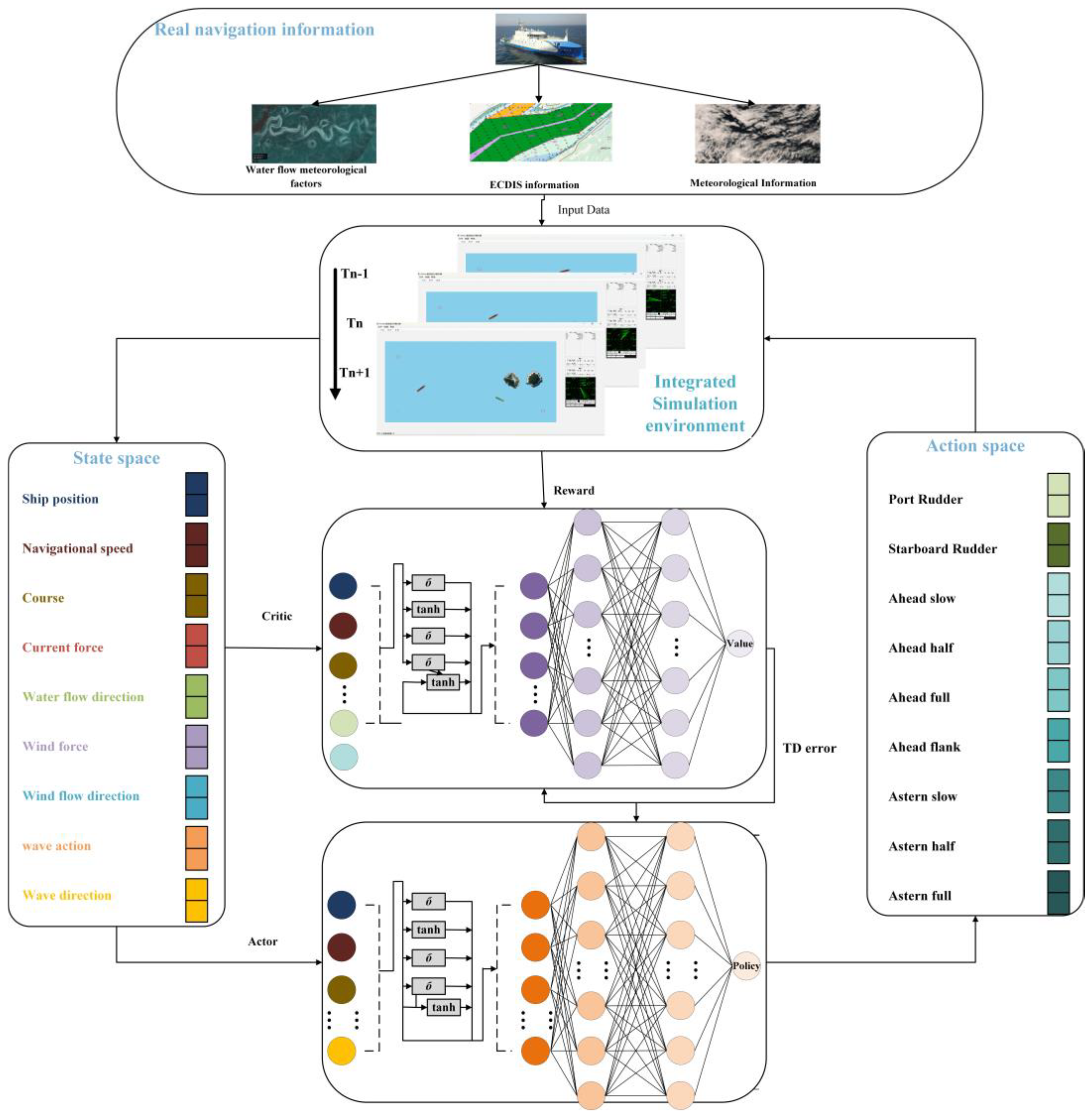
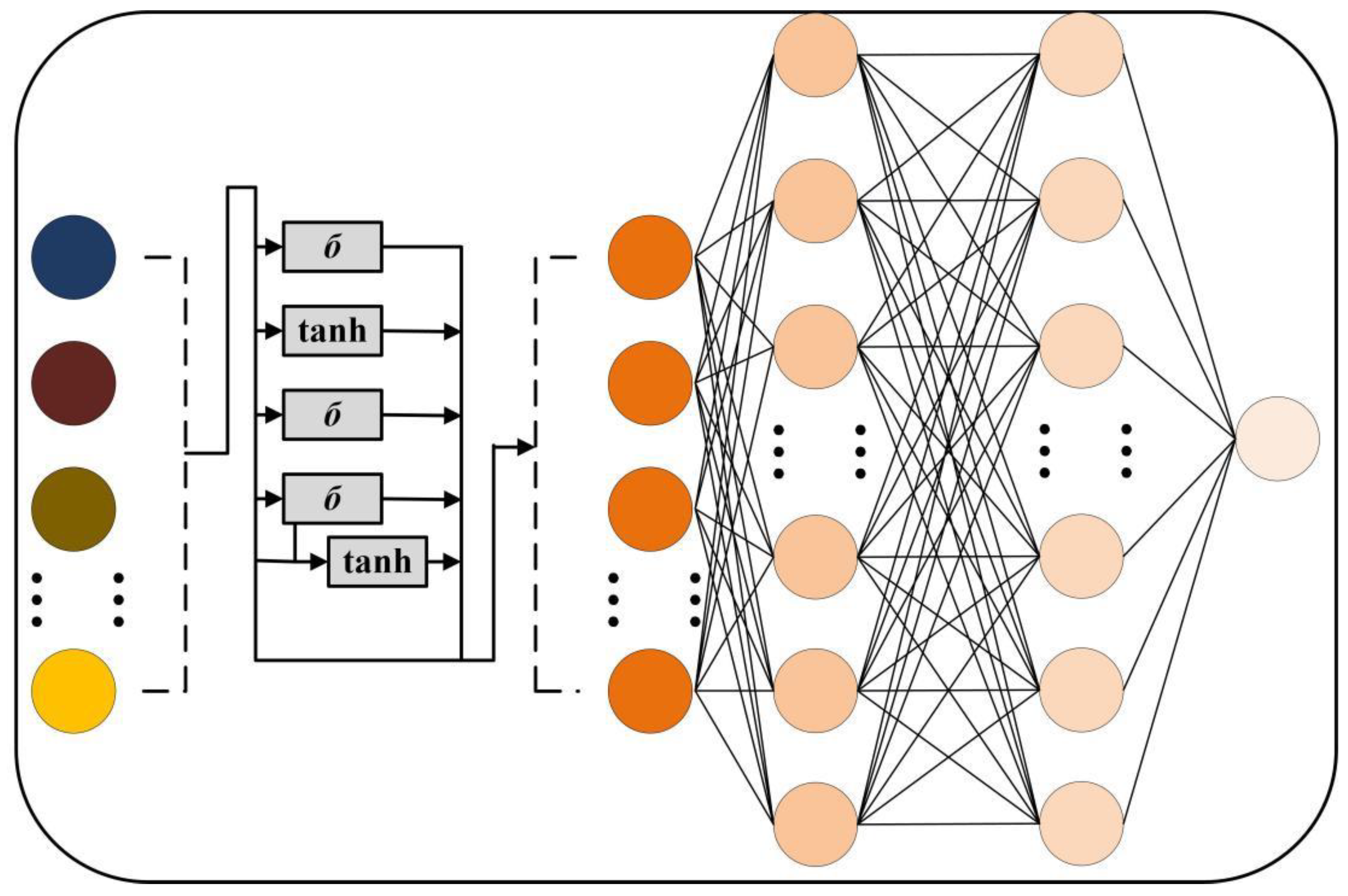
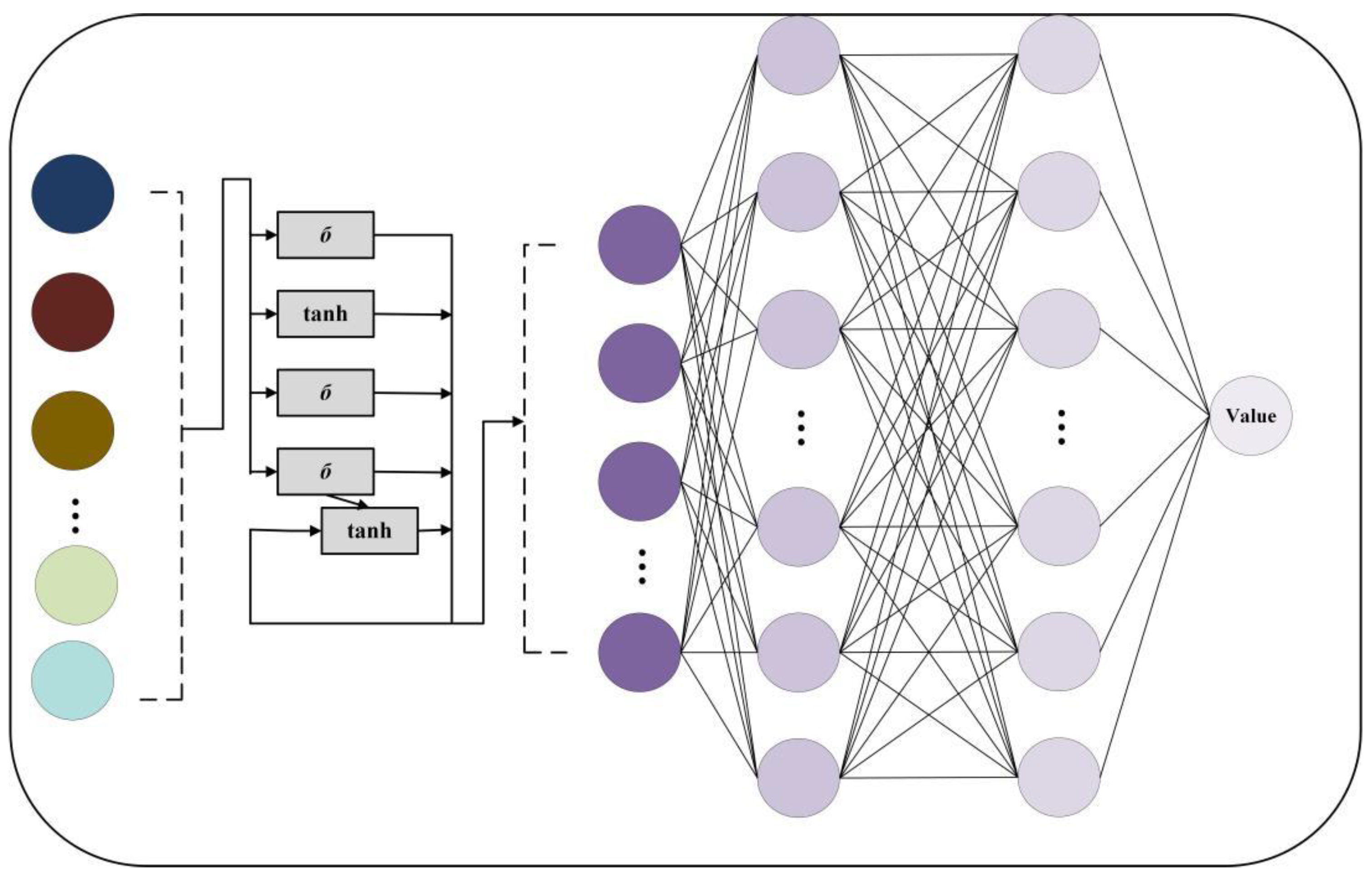
To address the limitations in existing research, this study aims to develop an intelligent decision-making model that accurately reflects real-world navigation data, thereby enhancing the autonomous navigation and collision avoidance capabilities of unmanned ships in complex marine environments. As shown in Figure 1, the system simulates real-world environmental factors, such as water currents, meteorological conditions, and electronic chart data (ECDIS), among others, to create a high-fidelity simulation environment. This enables the agent to train under dynamic conditions that closely resemble actual navigation scenarios. Within a reinforcement learning framework, the state space includes key environmental variables, such as ship position, speed, heading, flow fields, and wind/waves, allowing the agent to fully perceive the complexity of the external environment and optimize its decisions under varying meteorological and hydrodynamic conditions. The reinforcement learning architecture incorporates an Actor-Critic structure, where the Critic evaluates decision values and the Actor generates specific control commands (e.g., steering and engine control) through a policy network. This ensures the ship operates safely and efficiently while adhering to COLREGs. Reinforcement learning optimizes strategy through TD error, enhancing the agent’s collision avoidance and path planning abilities through continuous interactions. Ultimately, the system uses an end-to-end learning approach, enabling the unmanned ship to autonomously perceive, decide, and execute navigation tasks, thereby improving its adaptability and reliability in complex environments.

Figure 1 illustrates the overall architecture of the Adaptive Temporal Reinforcement Navigation Model (ATRNM) designed in this study for intelligent navigation decision-making in MASS. The model is built around an integrated simulation environment that replicates real-world navigation data, including water currents, meteorological conditions, ECDIS, and weather information. It interacts dynamically across multiple time steps (Tn − 1, Tn, Tn + 1). The state space incorporates external environmental variables, such as ship position, speed, heading, and wind/wave conditions. These data are processed by an Actor-Critic network, where the Critic evaluates the state value function and computes the TD error, while the Actor generates the optimal navigation strategy. Through the integration of LSTM networks, the model effectively captures temporal dependencies, improving its adaptability to complex and dynamic marine environments. The action space controls the ship’s rudder and propulsion system, adjusting the left and right rudders and varying forward and backward speeds to optimize the navigation path and ensure the effectiveness of the collision avoidance strategy. The overall architecture optimizes the strategy through a reinforcement learning framework (PPO), enabling the model to enhance its collision avoidance capabilities and navigation stability in dynamic environments, thereby providing efficient decision support for intelligent navigation in MASS.

The main contributions of this study are as follows:

First, the real-world ship navigation environment is accurately mapped into a reinforcement learning simulation environment through mathematical modeling. In this simulation, the unmanned ship is no longer modeled as a particle; instead, the forces exerted by the rudder and engine are applied to the ship’s stern. Furthermore, hydrometeorological factors are integrated into the environmental design. All relevant environmental information is incorporated into the state space, enabling the proposed PPO-LSTM model to gain a better understanding of the ship’s current navigation state. The LSTM’s processing of temporal information allows the unmanned ship to more effectively capture trends in the dynamic environment. This also helps mitigate potential issues of dimensionality explosion in the state space. Finally, incorporating the COLREGs into the reward function design ensures the practicality of the trained model.

The remainder of this study is organized as follows: Section 2 presents the preliminary work for the intelligent collision avoidance model, including the design of the simulation environment and the COLREG regulations. Section 3 describes the design of the unmanned ship’s intelligent decision-making model, which is trained using the policy gradient update method to develop a collision avoidance decision model. The model is trained with the improved PPO algorithm, and the designs of the state space, action space, and reward function are also detailed. Section 4 discusses the improved decision-making model, including algorithm enhancements and the construction of the temporal information network. Section 5 compares the model’s training performance in simulation experiments and presents the results of the trained strategy in the simulation environment. Finally, Section 6 provides conclusions and outlines future research directions.

2. Preliminary Preparations

This chapter introduces the design of the simulation environment and the regulations of COLREG. To accurately replicate the real-world navigation environment of ships in the reinforcement learning simulation, mathematical models of the ship and hydrometeorological factors are required. In the simulation environment, the forces exerted by hydrometeorological factors interact with the ship’s physical characteristics (e.g., propulsion, resistance), influencing its trajectory. Furthermore, COLREG requirements must be considered to ensure that the agent’s behavior adheres to legal regulations and safety standards in both simulated and real-world scenarios.

2.1. Modeling Real-World Complex Environments

During a ship’s voyage, hydrometeorological factors significantly influence its maneuverability. To effectively simulate these environmental effects, numerical methods based on physical models and stochastic processes are utilized. This section discusses the modeling of wind, waves, and currents, simplifying higher-order small quantities to reduce computational complexity, while retaining the influence of hydrometeorological factors on the ship’s maneuverability.

(1)

Simulation of wind

Wind affects the ship’s navigation path, speed, and stability. Under strong wind conditions, the lateral force exerted by the wind increases significantly, causing a deviation in the ship’s heading. In this model, both wind strength and direction are represented by a two-dimensional vector. The wind speed is controlled by a random number generator, with its magnitude fluctuating within a specified maximum wind speed range. Each time the simulation is updated, the wind direction is randomly selected within a range from 0 to 2π. This method of variation reflects the high degree of variability and randomness of wind in real-world conditions.

The mathematical expression for wind force is:

$${\mathrm{F}}_{\mathrm{wind}}=({\mathrm{v}}_{\mathrm{wind},\mathrm{x}},{\mathrm{v}}_{\mathrm{wind},\mathrm{y}})=(\mathrm{random}(-{\mathrm{v}}_{\max },{\mathrm{v}}_{\max }),\mathrm{random}(-{\mathrm{v}}_{\max },{\mathrm{v}}_{\max }\left)\right)$$

(1)

Here, F_wind represents the wind force magnitude; v_max denotes the maximum wind speed, which can be set during system initialization to account for severe sea conditions during model training. Random (−v_max, v_max) generates a random value within the specified wind speed range for simulating wind force.

The mathematical expression for wind direction is as follows:

$$\mathrm{W}=({\mathrm{w}}_{\mathrm{x}},{\mathrm{w}}_{\mathrm{y}})=(\mathrm{w}·\cos (\theta ),\mathrm{w}·\sin (\theta ))$$

(2)

Here, W represents the wind direction, and θ denotes the wind direction angle, measured in radians and randomly distributed within the range (0, 2π).

In the system, wind force updates follow a time-step process, where new values for wind speed and direction are randomly generated to simulate the continuous variation of wind.

(2)

Simulation of Currents

Ocean currents significantly affect the ship’s navigation path. In contrast to wind, the influence of currents is typically persistent and directional, meaning ocean currents generally change more gradually, though they may also cause long-term offset effects. In this system, the current is represented as a two-dimensional vector that describes its speed and direction.

The mathematical expression for the current force is as follows:

$${\mathrm{F}}_{\mathrm{current}}=({\mathrm{v}}_{\mathrm{current},\mathrm{x}},{\mathrm{v}}_{\mathrm{current},\mathrm{y}})$$

(3)

Here, F_current represents the magnitude of the current force; v_current,x and v_current,y represent the components of the current in the x-axis and y-axis directions, respectively. The principle is analogous to that of wind force.

The direction of the current is expressed as an angle. The initial direction is randomly generated within a specified range, and during each update, the direction is adjusted based on a given variance. This process allows for a change in the current’s direction, though not randomly; instead, the direction retains a certain degree of correlation.

The mathematical expression for the current direction is as follows:

$${\mathrm{F}}_{\mathrm{current}(\mathrm{t}+1)}={\mathrm{F}}_{\mathrm{current}}\left(\mathrm{t}\right)+\delta {\mathrm{F}}_{\mathrm{current}}$$

(4)

Here, F_current(t+1) represents the current direction at the next time step, while F_current(t) indicates the current direction at the present time step. δF_current denotes the adjustment, which is dependent on the current direction.

(3)

Wave Model

The influence of waves on maritime navigation is particularly pronounced, especially under adverse weather conditions, where wave forces can significantly affect vessel stability. The oscillatory effect of waves may induce vibrations during navigation, and in extreme cases, it can result in the vessel losing control or sustaining damage. Therefore, wave impacts must be carefully considered in the design of MASS.

The mathematical expression for wave force is as follows:

$${\mathrm{F}}_{\mathrm{wave}}=({\mathrm{V}}_{\mathrm{wave},\mathrm{x}},{\mathrm{V}}_{\mathrm{wave},\mathrm{y}})$$

(5)

Here, F_wave represents the wave force, while V_wave,x and V_wave,y denote the magnitudes of the wave force in the x-axis and y-axis directions, respectively.

The wave magnitude fluctuates periodically at a fixed frequency during each update, and the wave direction is random. The wave update formula is as follows:

$${\mathrm{F}}_{\mathrm{w}\mathrm{a}\mathrm{v}\mathrm{e}}\left(\mathrm{t}\right)=\left\{\begin{array}{c}\mathrm{r}\mathrm{a}\mathrm{n}\mathrm{d}\mathrm{o}\mathrm{m}\left(-{\mathrm{v}}_{\mathrm{w}\mathrm{a}\mathrm{v}\mathrm{e},\mathrm{m}\mathrm{a}\mathrm{x}},{\mathrm{v}}_{\mathrm{w}\mathrm{a}\mathrm{v}\mathrm{e},\mathrm{m}\mathrm{a}\mathrm{x}}\right)\\ \left(\mathrm{0,0}\right)\end{array}\right.\begin{array}{c}\mathrm{i}\mathrm{f} \mathrm{t} \mathrm{m}\mathrm{o}\mathrm{d} \mathrm{w}\mathrm{a}\mathrm{v}\mathrm{e} \mathrm{f}\mathrm{r}\mathrm{e}\mathrm{q}\mathrm{u}\mathrm{e}\mathrm{n}\mathrm{c}\mathrm{y}<\mathsf{ϵ}\\ \mathrm{o}\mathrm{t}\mathrm{h}\mathrm{e}\mathrm{r}\mathrm{w}\mathrm{i}\mathrm{s}\mathrm{e}\end{array}$$

(6)

Here, ϵ is the threshold used to determine whether the wave’s influence is updated at the current time step.

2.2. Modeling for Realistic Ship Maneuvering

This section explores the process of developing ship maneuvering models, with a particular emphasis on hydrodynamic modeling and the mathematical representation of maneuvering dynamics. We begin by analyzing the six degrees of freedom in ship motion and then focus on key maneuvers involved in collision avoidance, such as forward motion, yaw, and heave. By constructing a ship motion diagram in a still-water coordinate system, we introduce key parameters of maneuverability, including rudder angle input, yaw response, and the maneuverability index. Additionally, this section discusses how hydrometeorological factors are incorporated into the ship’s dynamic model.

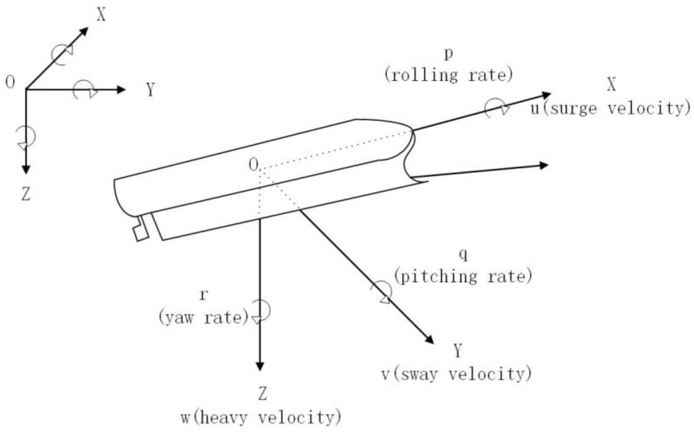
The motion of a ship is inherently complex and typically exhibits six degrees of freedom. As shown in Figure 2, these motions consist of three translational movements along the body-fixed coordinate axes and three rotational movements around these axes. The translational motions include forward speed along the X-axis, lateral speed along the Y-axis, and heaving speed along the Z-axis. The rotational motions include pitch angular velocity along the X-axis, roll angular velocity along the Y-axis, and yaw angular velocity along the Z-axis. During collision avoidance, the primary focus is on the ship’s forward motion, drift, and pitch. In contrast, heaving, yawing, and rolling motions have relatively minor effects.

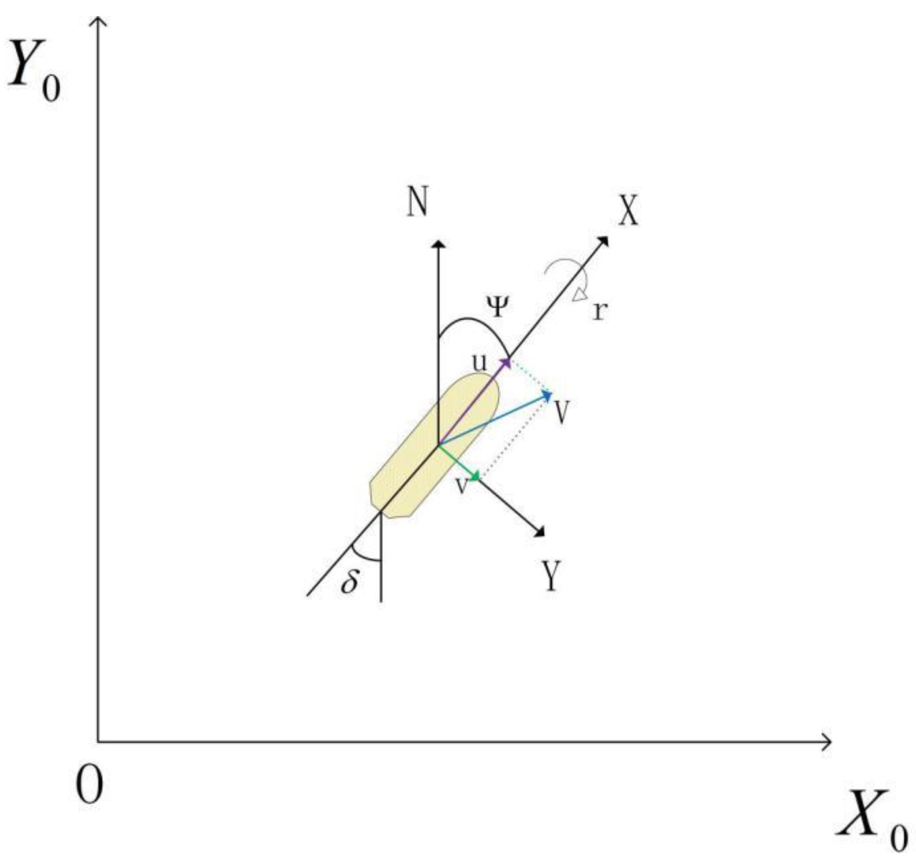
In Figure 3, the coordinate system X₀OY₀ represents the still-water coordinate system, with the X-axis aligned along the ship’s length, the Y-axis perpendicular to the X-axis, and N denoting the true north direction. In the X-direction, the ship’s pitch velocity and forward motion are considered, while the Y-direction represents the ship’s drift motion. The variable V indicates the actual direction of the ship’s motion. Ψ represents the ship’s heading, and β denotes the rudder angle. Here, only the ship’s drift and pitch motions are considered, and the resulting mathematical model is as follows:

$$\left[\begin{array}{c}\dot{\mathrm{v}}\\ \dot{\mathrm{r}}\end{array}\right]=\left[\begin{array}{cc}{\mathrm{a}}_{11}& {\mathrm{a}}_{12}\\ {\mathrm{a}}_{21}& {\mathrm{a}}_{22}\end{array}\right]\left[\begin{array}{c}\mathrm{v}\\ \mathrm{r}\end{array}\right]+\left[\begin{array}{c}{\mathrm{b}}_{11}\\ {\mathrm{b}}_{21}\end{array}\right]\delta$$

(7)

In Equation (7), δ represents the ship’s rudder angle input, and the coefficients a11, a12, a21, a22, b11, and b21 are determined by the ship’s basic parameters. The equation can be transformed into a simplified expression describing the effect of the rudder on the ship’s pitch response, as follows:

$${\mathrm{T}}_1{\mathrm{T}}_2\ddot{\mathrm{r}}+({\mathrm{T}}_1+{\mathrm{T}}_2)\dot{\mathrm{r}}+\mathrm{r}=\mathrm{K}\delta +\mathrm{K}{\mathrm{T}}_3\dot{\delta }$$

(8)

In Equation (8), K, T₁, T₂, and T₃ are maneuverability indices, which can be estimated using the ship’s basic parameters a11, a12, a21, a22, b11, and b21. Taking the Laplace transform of Equation (8) yields the transfer function, as expressed in Equation (9).

$${\mathrm{G}}_{\mathrm{r}\delta }(\mathrm{s})={\displaystyle \frac{\mathrm{r}(\mathrm{s})}{\delta (\mathrm{s})}}={\displaystyle \frac{\mathrm{K}(1+{\mathrm{T}}_{3^{\mathrm{S}}})}{(1+{\mathrm{T}}_{1^{\mathrm{S}}})(1+{\mathrm{T}}_{2^{\mathrm{S}}})}}$$

(9)

For a ship, which is a high-inertia vehicle, its dynamic characteristics are valid only in the low-frequency range. Therefore, we set s = jω→0, and after performing a series expansion while neglecting second and third order terms, we obtain the Nomoto model, as follows:

$${\mathrm{G}}_{\mathrm{r}\delta }(\mathrm{s})={\displaystyle \frac{\mathrm{K}}{1+{\mathrm{T}}_{\mathrm{S}}}}$$

(10)

Based on the relationship $\mathrm{r}=\dot{\psi }$, we replace r in Equation (10) with the ship’s heading angle ψ, resulting in the corresponding equation:

$${\mathrm{G}}_{\mathrm{r}\delta }(\mathrm{s})={\displaystyle \frac{\mathrm{K}}{1+{\mathrm{T}}_{\mathrm{S}}}}$$

(11)

$$\mathrm{T}\ddot{\psi }+\dot{\psi }=\mathrm{K}\delta$$

(12)

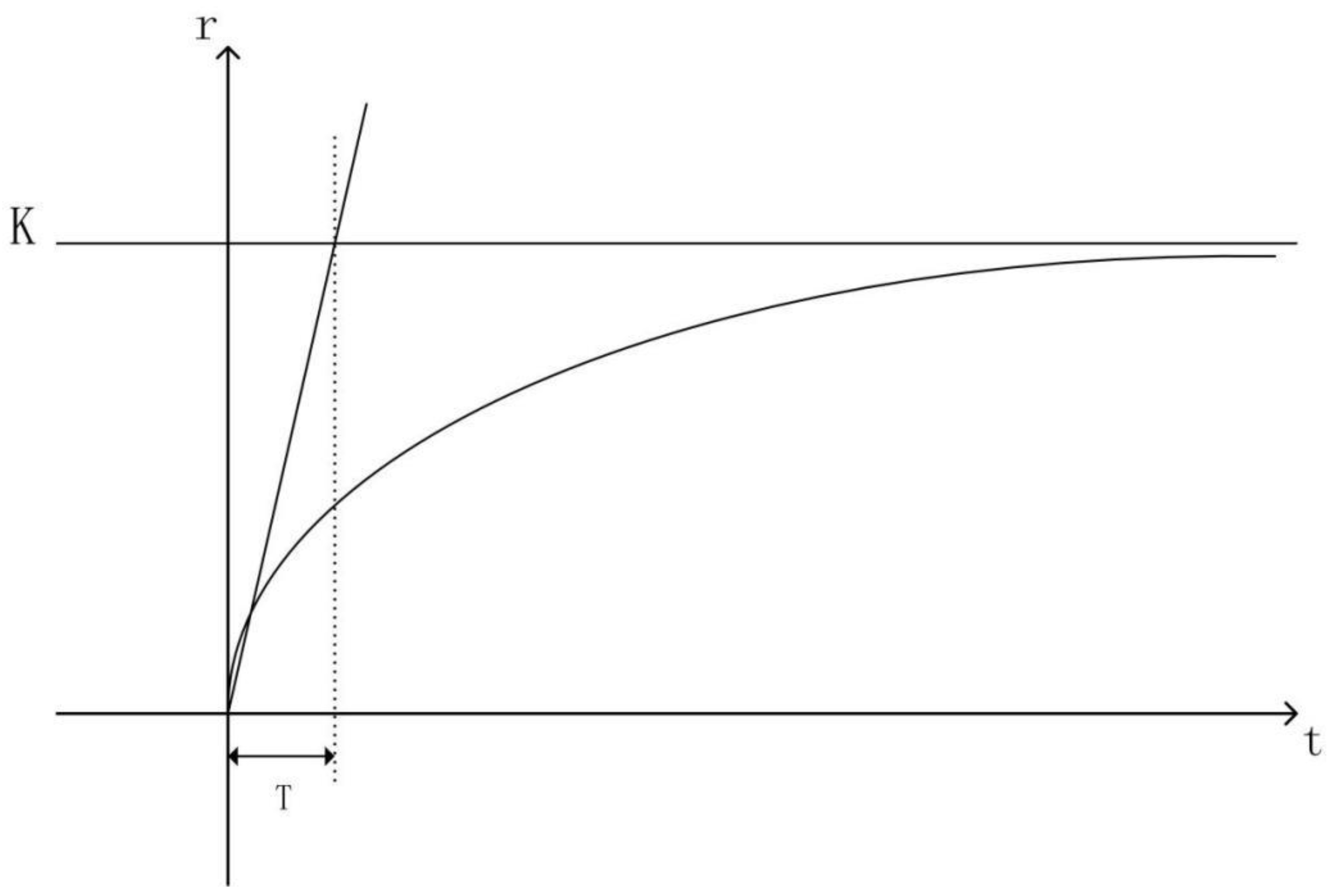
Equation (12) represents the first-order K-T equation for ship maneuvering. Figure 4 illustrates the output response of the first-order Nomoto model, clearly demonstrating the physical significance of the K and T indices. K represents the factor influencing the turning rate after the ship takes control; a larger K results in a higher turning rate, indicating better maneuverability. T denotes the key factor in determining the time required to reach the maximum turning rate, referred to as the time constant.

Considering the ship as a rigid body, as shown in Figure 4, when the ship steers with an arbitrary rudder angle $\delta$, the turning rate r is given by the formula above, which can be regarded as the ship’s steering motion equation. When the ship has a rudder angle input for steering, assuming its initial conditions are t = 0, $\delta$ = $\delta$₀, and r = 0, the yaw angle at any given time can be calculated using the KT formula in Equation (12):

$$\mathrm{r}=\mathrm{K}\delta (1-{\mathrm{e}}^{-\mathrm{t}/\mathrm{T}})$$

(13)

The ship’s heading is the time derivative of the yaw angle, and its relationship is as follows:

$$\psi =\mathrm{K}{\delta }_0(\mathrm{t}-\mathrm{T}+\mathrm{T}·{\mathrm{e}}^{-\mathrm{t}/\mathrm{T}})$$

(14)

The advantages of using the Nomoto model to develop the ship’s hydrodynamic model for simulation training are:

• The Nomoto model simplifies higher-order infinitesimals, resulting in a lower-order ship motion control model, which enhances computational efficiency and simulation accuracy.
• While the Nomoto model simplifies higher-order terms and the low-frequency range, the results from the low-frequency range in actual simulations closely align with those from higher-order models, ensuring the authenticity of the experiments.

Based on the previously introduced hydrodynamic model, a new ship motion model is proposed that integrates external environmental factors, including the ship’s rudder effect, propeller acceleration effect, and the influence of environmental factors such as wind speed, waves, and currents on ship motion.

(1)

Ship Motion Model Design

The ship’s motion can be represented by a dynamic model, typically governed by Newton’s second law, while accounting for both linear and nonlinear responses. Based on this, we assume that the ship’s motion on the water surface is described by variables such as velocity, position, and heading angle. The equation of motion for the ship can be expressed as follows:

$${\displaystyle \frac{\mathrm{d}\mathrm{r}(\mathrm{t})}{\mathrm{d}\mathrm{t}}}=\left({\displaystyle \genfrac{}{}{0pt}{}{\dot{\mathrm{x}}(\mathrm{t})}{\dot{\mathrm{y}}(\mathrm{t})}}\right)=\mathrm{v}\left(\mathrm{t}\right)\left({\displaystyle \genfrac{}{}{0pt}{}{\cos \left(\theta \left(\mathrm{t}\right)\right)}{\sin \left(\theta \left(\mathrm{t}\right)\right)}}\right)$$

(15)

Here, r(t) represents the ship’s position vector in a two-dimensional space, which varies over time t; $\dot{\mathrm{x}}\left(\mathrm{t}\right),\dot{\mathrm{y}}(\mathrm{t})$ represent the velocity components along the x-axis and y-axis are denoted, while v(t) represents the ship’s current speed.

The rudder effect is a key factor influencing the ship’s steering. Equations (13) and (14) quantify the rudder effect on steering for different ship types, based on the ship’s KT index. We considered six ship types, including tankers, fishing vessels, and passenger ships, to comprehensively assess the impact of varying maneuverability on collision avoidance.

Additionally, the ship’s speed variation is influenced by the propeller’s rotational speed and the power system’s efficiency. Let n(t) represent the propeller speed, and the propeller’s acceleration a(t) can be calculated using the propeller’s efficiency, the ship’s current speed v(t), and environmental resistance.

$$\mathrm{a}(\mathrm{t})={\mu }_{\mathrm{p}\mathrm{r}\mathrm{o}\mathrm{p}}·\mathrm{n}\left(\mathrm{t}\right)-\mathrm{D}\left(\mathrm{v}\left(\mathrm{t}\right)\right)$$

(16)

Here, $\mathrm{D}\left(\mathrm{v}\left(\mathrm{t}\right)\right)$ refers to the ship’s total resistance, which is typically influenced by factors such as the ship’s type and speed.

(2)

Ship Resistance Model Design

The primary resistance model considered for the ship includes viscous resistance (D_viscous(v(t))), wave resistance (D_wave(v(t))), air resistance (D_air(v(t))), and additional resistance (D_extra(v(t))). The specific mathematical expressions are as follows:

$$\begin{array}{c}\mathrm{D}(\mathrm{v}(\mathrm{t}))={\mathrm{D}}_{\mathrm{v}\mathrm{i}\mathrm{s}\mathrm{c}\mathrm{o}\mathrm{u}\mathrm{s}}(\mathrm{v}(\mathrm{t}))+{\mathrm{D}}_{\mathrm{w}\mathrm{a}\mathrm{v}\mathrm{e}}(\mathrm{v}(\mathrm{t}))+{\mathrm{D}}_{\mathrm{a}\mathrm{i}\mathrm{r}}(\mathrm{v}(\mathrm{t}))+{\mathrm{D}}_{\mathrm{e}\mathrm{x}\mathrm{t}\mathrm{r}\mathrm{a}}(\mathrm{v}(\mathrm{t}))\\ ={\mathrm{C}}_{\mathrm{v}\mathrm{i}\mathrm{s}\mathrm{c}\mathrm{o}\mathrm{u}\mathrm{s}}·{\mathrm{v}(\mathrm{t})}^2+{\mathrm{C}}_{\mathrm{w}\mathrm{a}\mathrm{v}\mathrm{e}}·{\mathrm{v}(\mathrm{t})}^{1.5}+{\mathrm{C}}_{\mathrm{a}\mathrm{i}\mathrm{r}}·{\mathrm{v}(\mathrm{t})}^2+{\mathrm{C}}_{\mathrm{e}\mathrm{x}\mathrm{t}\mathrm{r}\mathrm{a}}·{\mathrm{v}(\mathrm{t})}^2\end{array}$$

(17)

Here, $\mathrm{D}(\mathrm{v}(\mathrm{t}))$ represents the total resistance; C_viscous is the viscous resistance coefficient related to the ship’s shape and the properties of the water body; C_wave is the coefficient associated with the ship’s speed, shape, and the wave characteristics of the water body; C_air is the coefficient related to air density and the ship’s surface characteristics; and C_extra is the coefficient linked to the ship’s design and dynamic characteristics.

(3)

Interference from External Environmental Factors

We quantified the hydrometeorological factors discussed in Section 2.1 and integrated them with the ship’s dynamic model to derive the expression for the interference from external environmental factors as follows:

The influence of wind on ship motion is primarily reflected in the applied torque and resistance. Wind speed (V_wind’) and wind direction (${\theta }_{\mathrm{w}\mathrm{i}\mathrm{n}\mathrm{d}}$) influence the ship’s speed and heading, especially as the ship’s hull near the water surface experiences considerable wind pressure. The mathematical expression for the effect of wind on the ship’s speed and heading is given as follows:

$$\begin{array}{c}{{\mathrm{V}}_{\mathrm{w}\mathrm{i}\mathrm{n}\mathrm{d}}}^{\prime }={\mathrm{C}}_{\mathrm{w}\mathrm{i}\mathrm{n}\mathrm{d}}·{\mathrm{V}}_{\mathrm{w}\mathrm{i}\mathrm{n}\mathrm{d}}·\cos ({\theta }_{\mathrm{w}\mathrm{i}\mathrm{n}\mathrm{d}}-{\theta }_{\mathrm{s}\mathrm{h}\mathrm{i}\mathrm{p}})\\ ={\mathrm{C}}_{\mathrm{w}\mathrm{i}\mathrm{n}\mathrm{d}}·{\mathrm{V}}_{\mathrm{w}\mathrm{i}\mathrm{n}\mathrm{d}}·\cos ({\mathrm{C}}_{\mathrm{w}\mathrm{i}\mathrm{n}\mathrm{d}\_\mathrm{t}\mathrm{o}\mathrm{r}\mathrm{q}\mathrm{u}\mathrm{e}}·{\mathrm{V}}_{\mathrm{w}\mathrm{i}\mathrm{n}\mathrm{d}}·\sin ({\theta }_{\mathrm{w}\mathrm{i}\mathrm{n}\mathrm{d}}-{\theta }_{\mathrm{s}\mathrm{h}\mathrm{i}\mathrm{p}})-{\theta }_{\mathrm{s}\mathrm{h}\mathrm{i}\mathrm{p}})\end{array}$$

(18)

Here, V_wind’ represents the change in ship speed due to wind; C_wind is the wind influence coefficient on the ship, which depends on the ship’s type and the wind-exposed area of the hull; V_wind is the wind speed; $\theta$_wind is the wind direction (the angle between the wind direction and the ship’s heading); $\theta$_ship is the ship’s heading; ${\mathrm{C}}_{\mathrm{w}\mathrm{i}\mathrm{n}\mathrm{d}\_\mathrm{t}\mathrm{o}\mathrm{r}\mathrm{q}\mathrm{u}\mathrm{e}}$ is the wind torque influence coefficient.

The effect of the current is a significant external factor influencing the ship’s speed and heading. The current velocity (V_current) and direction ($\theta$_current) combine to affect the ship’s motion by altering its velocity and direction. The mathematical expression for the impact of the current on the ship’s speed and heading is as follows:

$$\begin{array}{c}{{\mathrm{V}}_{\mathrm{c}\mathrm{u}\mathrm{r}\mathrm{r}\mathrm{e}\mathrm{n}\mathrm{t}}}^{\prime }={\mathrm{C}}_{\mathrm{c}\mathrm{u}\mathrm{r}\mathrm{r}\mathrm{e}\mathrm{n}\mathrm{t}}·{\mathrm{V}}_{\mathrm{c}\mathrm{u}\mathrm{r}\mathrm{r}\mathrm{e}\mathrm{n}\mathrm{t}}·\cos \left({\theta }_{\mathrm{c}\mathrm{u}\mathrm{r}\mathrm{r}\mathrm{e}\mathrm{n}\mathrm{t}}-{\theta }_{\mathrm{s}\mathrm{h}\mathrm{i}\mathrm{p}}\right)\\ ={\mathrm{C}}_{\mathrm{c}\mathrm{u}\mathrm{r}\mathrm{r}\mathrm{e}\mathrm{n}\mathrm{t}}·{\mathrm{V}}_{\mathrm{c}\mathrm{u}\mathrm{r}\mathrm{r}\mathrm{e}\mathrm{n}\mathrm{t}}·\cos \left({\mathrm{C}}_{\mathrm{c}\mathrm{u}\mathrm{r}\mathrm{r}\mathrm{e}\mathrm{n}\mathrm{t}\_\mathrm{t}\mathrm{o}\mathrm{r}\mathrm{q}\mathrm{u}\mathrm{e}}·{\mathrm{V}}_{\mathrm{c}\mathrm{u}\mathrm{r}\mathrm{r}\mathrm{e}\mathrm{n}\mathrm{t}}·\sin \left({\theta }_{\mathrm{c}\mathrm{u}\mathrm{r}\mathrm{r}\mathrm{e}\mathrm{n}\mathrm{t}}-{\theta }_{\mathrm{s}\mathrm{h}\mathrm{i}\mathrm{p}}\right)-{\theta }_{\mathrm{s}\mathrm{h}\mathrm{i}\mathrm{p}}\right)\end{array}$$

(19)

Here, V_current’ represents the change in ship speed due to the current; C_current is the current influence coefficient; V_current denotes the current speed; $\theta$_current and $\theta$_ship represent the directions of the current and the ship’s heading, respectively; and ${\mathrm{C}}_{\mathrm{c}\mathrm{u}\mathrm{r}\mathrm{r}\mathrm{e}\mathrm{n}\mathrm{t}\_\mathrm{t}\mathrm{o}\mathrm{r}\mathrm{q}\mathrm{u}\mathrm{e}}$ is the current torque influence factor.

The impact of waves primarily manifests in two ways: first, the wave height affects the ship’s pitch; second, the energy of the waves is transmitted through the hull, subsequently altering the ship’s heading and speed. Since the effect of pitch on collision avoidance is minimal, it can be disregarded. Therefore, we simplify the wave impact as the relationship between wave height, wavelength, and the ship’s speed and heading. The mathematical expression is as follows:

$$\begin{array}{c}{\mathrm{V}}_{\mathrm{w}\mathrm{a}\mathrm{v}\mathrm{e}}={\mathrm{C}}_{\mathrm{w}\mathrm{a}\mathrm{v}\mathrm{e}}·{\mathrm{H}}_{\mathrm{w}\mathrm{a}\mathrm{v}\mathrm{e}}·\cos \left({\theta }_{\mathrm{w}\mathrm{a}\mathrm{v}\mathrm{e}}-{\theta }_{\mathrm{s}\mathrm{h}\mathrm{i}\mathrm{p}}\right)\\ ={\mathrm{C}}_{\mathrm{w}\mathrm{a}\mathrm{v}\mathrm{e}}·{\mathrm{H}}_{\mathrm{w}\mathrm{a}\mathrm{v}\mathrm{e}}·\cos \left({\mathrm{C}}_{\mathrm{w}\mathrm{a}\mathrm{v}\mathrm{e}\_\mathrm{t}\mathrm{a}\mathrm{r}\mathrm{q}\mathrm{u}\mathrm{e}}·{\mathrm{H}}_{\mathrm{w}\mathrm{a}\mathrm{v}\mathrm{e}}·\sin \left({\theta }_{\mathrm{w}\mathrm{a}\mathrm{v}\mathrm{e}}-{\theta }_{\mathrm{s}\mathrm{h}\mathrm{i}\mathrm{p}}\right)-{\theta }_{\mathrm{s}\mathrm{h}\mathrm{i}\mathrm{p}}\right)\end{array}$$

(20)

Here, V_wave represents the change in ship speed due to the waves; C_wave is the wave influence coefficient, which primarily depends on the ship’s shape and the wave frequency; H_wave denotes the wave height; $\theta$_wave and $\theta$_ship represent the wave direction and the ship’s heading, respectively; and ${\mathrm{C}}_{\mathrm{w}\mathrm{a}\mathrm{v}\mathrm{e}\_\mathrm{t}\mathrm{a}\mathrm{r}\mathrm{q}\mathrm{u}\mathrm{e}}$ is the wave torque influence factor.

2.3. COLREG Rules

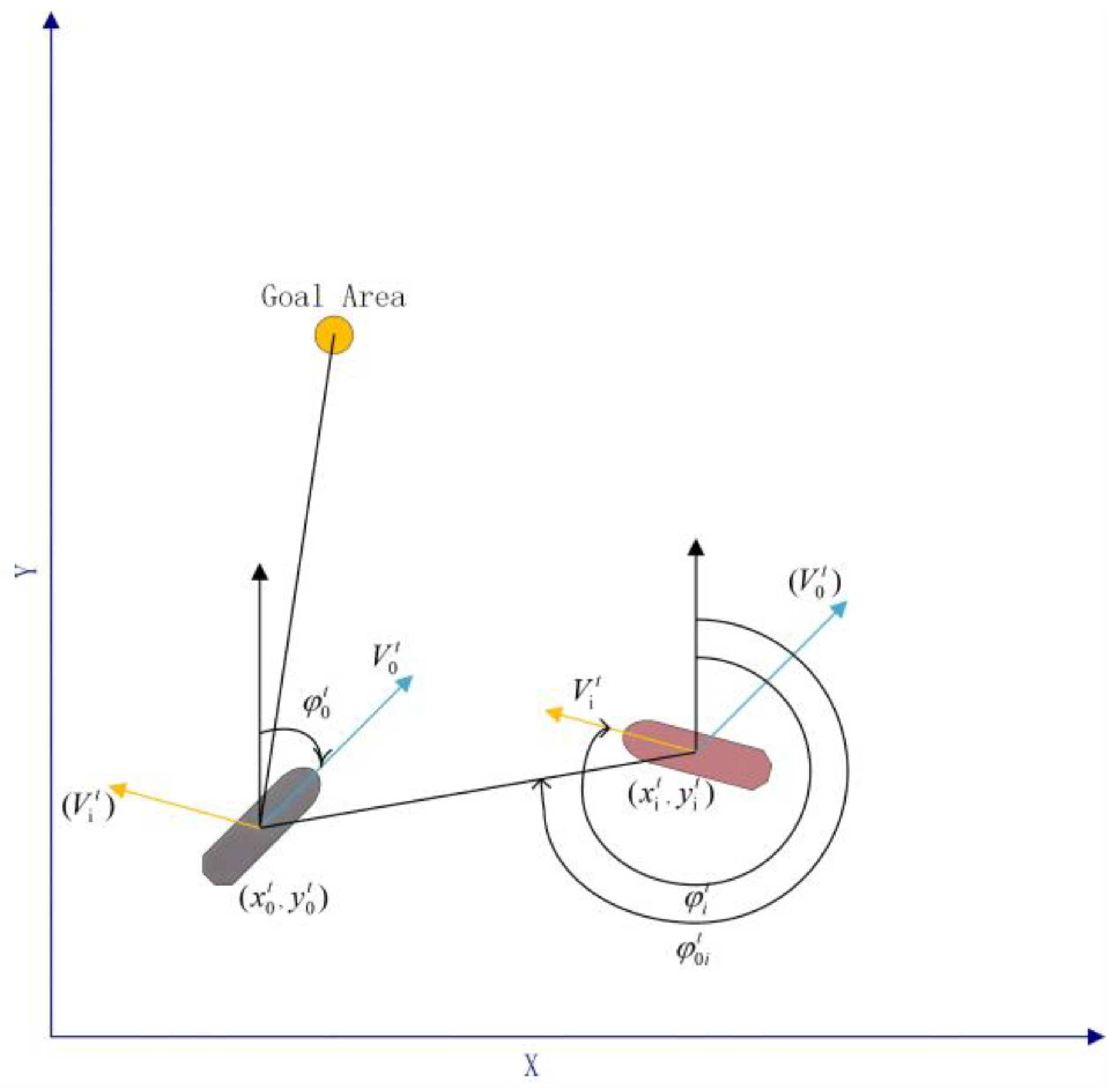
The first step in collision risk assessment is to evaluate the potential for collision. According to the COLREGs, “every ship should use all available means to assess the risk of collision under the prevailing environmental conditions”. In practice, collision risks are often evaluated based on the Time to Closest Point of Approach (TCPA) and Closest Point of Approach (CPA) warnings displayed on electronic charts. In Figure 5, the two ships are identified as presenting a collision risk, which necessitates the calculation of TCPA and CPA to determine the likelihood of a collision.

Based on the relationships between DCPA and MINDCPA, as well as TCPA and MINTCPA, ships on the radar can be classified into three categories: (1) when DCPA > MINDCPA and TCPA > MINTCPA, the target ship is deemed safe and no collision risk exists; (2) when DCPA < MINDCPA and TCPA < MINTCPA, the target ship is considered dangerous but not immediately threatening, and evasive action should be considered; (3) when DCPA < MINDCPA and TCPA < MINTCPA, the target ship is highly dangerous, and immediate evasive action is required.

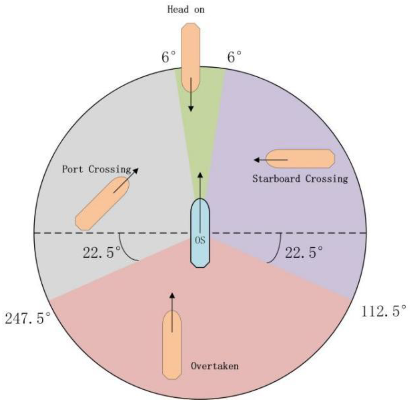
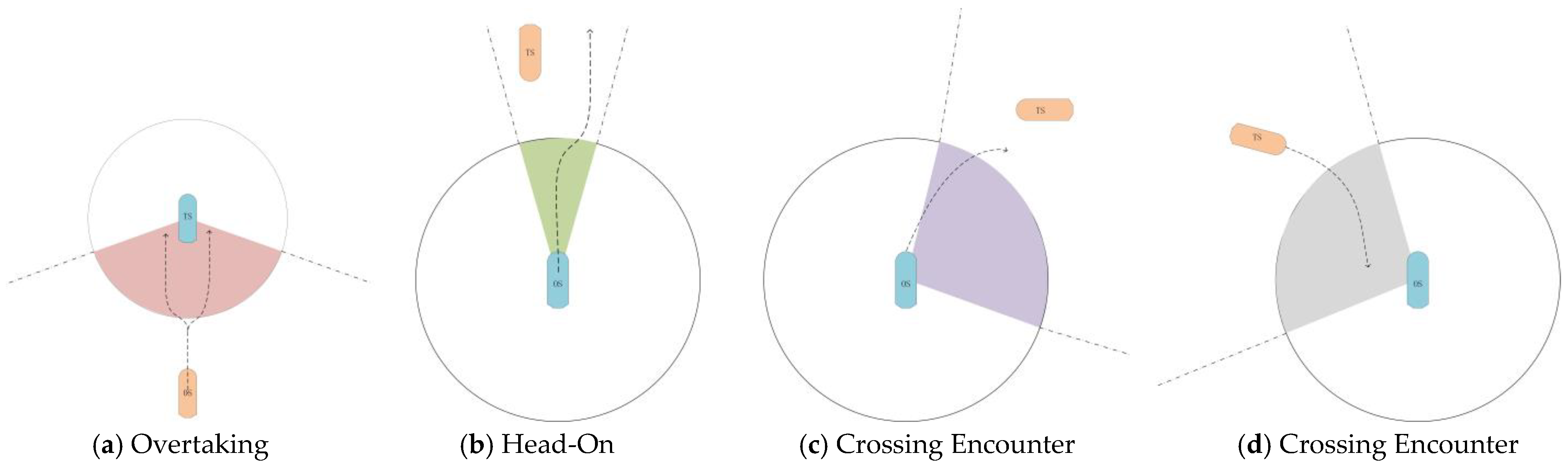
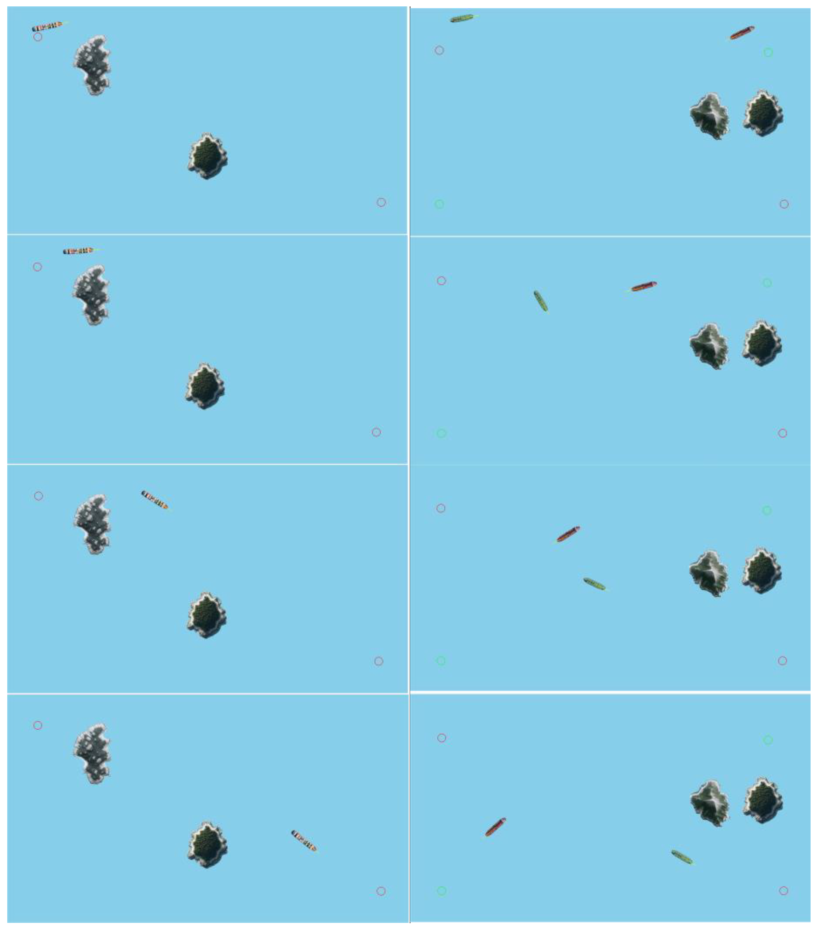
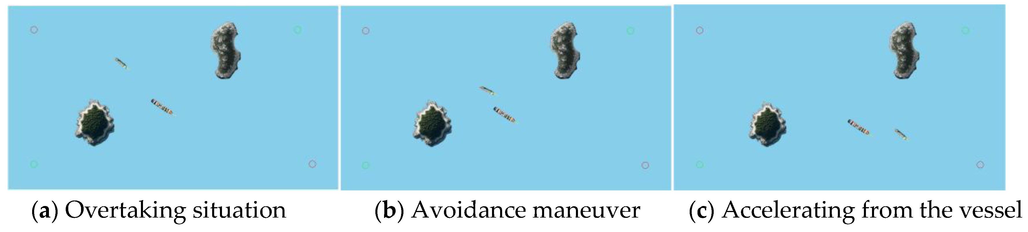
After assessing the collision risk between two ships, it is essential to evaluate their encounter situation, as shown in Figure 6. Based on the relative positions of the target ship and the own ship, the encounter can be classified into four types. Depending on the specific encounter, the own ship must take appropriate collision avoidance measures in accordance with the rules. As shown in Figure 7a, when a ship approaches another vessel from 22.5° to its stern, the ships are in an overtaking situation. The overtaking vessel must yield to the vessel ahead. 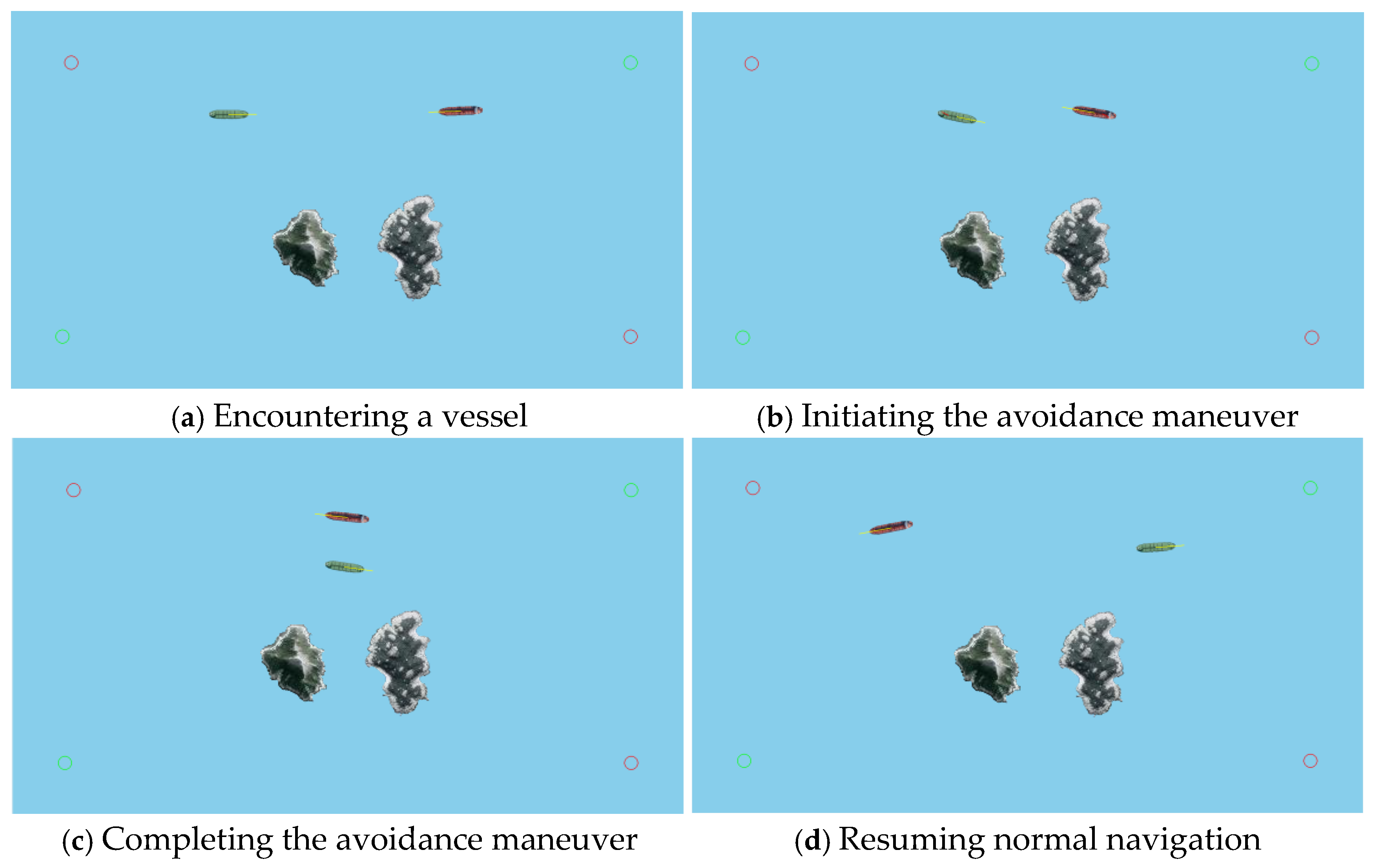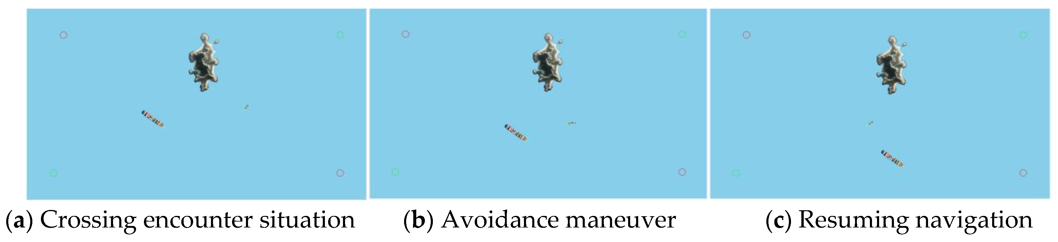Figure 7b illustrates that when two motorized ships meet on opposite or nearly opposite courses, creating a collision risk, they must pass each other on the left side. In the case of a crossing collision risk between the two ships, the right-of-way and give-way relationship must first be determined. As shown in Figure 7c, when the target ship is positioned on the right side of the own ship (6° to 112.5°), the own ship is the give-way vessel, and the target ship is the stand-on vessel. The own ship should actively steer to the right and pass the target ship on the left side. Figure 7d shows that when the target ship is positioned on the left side of the own ship (247.5° to 354°), the own ship is the stand-on vessel, and the target ship is the give-way vessel. The target ship should actively steer to the right and pass the own ship on the left side.

3. Methodology

3.1. Definition of State Space and Action Space

In the context of state space, a more complex configuration can provide a clearer description of the agent’s actual environment. However, overly redundant state space configurations can lead to erroneous strategy choices during training, as they may introduce irrelevant state factors. Thus, it is crucial to select the necessary and comprehensive state values for the state space. Based on the simulation environment designed in Chapter 2, we categorize the state space into maritime environmental information, which includes “wind, waves, and currents”. These are represented by vectors in both the X and Y axes, resulting in a total of six vectors. The state space also includes navigation information such as “ship position, heading, and speed”, with each ship having six parameters of navigation data. Furthermore, the state space incorporates information about the positions of obstacles and target points within the environment.

In this experiment, we use a continuous action space. The action space is defined by changes in “throttle” and “rudder angle”. Compared to previous discrete action spaces that limit the ship’s motion to directions like up, down, left, or right, the continuous action space introduces a delayed change in the ship’s motion state. This design aligns with real-world navigation inputs and more accurately reflects the ship’s actual motion states. Additionally, the trained model produces smooth trajectories during navigation in the simulation environment, ensuring compliance with maritime requirements.

3.2. Calculation of the Reward Function

The reward function is designed to direct the agent’s training process towards convergence in alignment with the desired objectives. In this model, the reward function (Equation (21)) comprises three components: navigation, posture, and safety rewards.

$$\mathrm{R}={\mathrm{R}}_{\mathrm{s}}+{\mathrm{R}}_{\mathrm{p}}+{\mathrm{R}}_{\mathrm{N}}$$

(21)

(a)

Navigation Rewards

The navigation reward R_N is designed to assist the autonomous ship in perceiving both the direction and distance to its destination in an unknown environment. It focuses on the ship’s navigation path and its progress toward reaching the destination. Therefore, the navigation reward is divided into three components: the distance reward r_d, the progress reward r_c, and the destination achievement reward r_g. The distance reward r_d is calculated based on the real-time distance between the ship and the target point, offering continuous directional guidance to the agent. The progress reward r_c reinforces the continuity of the voyage, preventing the ship from wandering or deviating from its course. The destination achievement reward r_g explicitly defines the ship’s destination. The specific reward function is as follows:

$${\mathrm{r}}_{\mathrm{d}}=-{\displaystyle \frac{{\mathrm{d}}_{\mathrm{c}}}{1000}}$$

(22)

$${\mathrm{r}}_{\mathrm{c}}=0.2,\mathrm{if} {\mathrm{d}}_{\mathrm{c}}<{\mathrm{d}}_{\mathrm{l}}$$

(23)

$${\mathrm{r}}_{\mathrm{g}}=20,\mathrm{if} {\mathrm{d}}_{\mathrm{c}}<50$$

(24)

$${\mathrm{R}}_{\mathrm{N}}={\mathrm{r}}_{\mathrm{d}}+{\mathrm{r}}_{\mathrm{c}}+{\mathrm{r}}_{\mathrm{g}}$$

(25)

(b)

Posture rewards

The attitude-related reward RP ensures that the actions taken during the autonomous ship’s navigation adhere to maritime requirements. This enables the agent to not only maintain stable heading control and speed regulation during training but also achieve the ideal docking posture upon reaching the target. The attitude-related rewards are categorized into heading reward r_a, speed reward r_v, and final posture reward r_f. The heading reward r_a is calculated based on the angle between the ship and the target point, guiding the agent to learn smooth steering control and avoid abrupt rudder angle changes. The speed reward r_v encourages the agent to develop reasonable acceleration and deceleration patterns by setting the optimal cruising speed. Finally, the final posture reward r_f ensures that the ship reduces its speed upon reaching its destination. The specific reward functions are as follows:

$${\theta }_{\mathrm{t}\mathrm{a}\mathrm{r}\mathrm{g}\mathrm{e}\mathrm{t}}={\mathrm{t}\mathrm{a}\mathrm{n}}^{-1}\left({\displaystyle \frac{{\mathrm{y}}_{\mathrm{t}\mathrm{a}\mathrm{r}\mathrm{g}\mathrm{e}\mathrm{t}}-\mathrm{y}}{{\mathrm{x}}_{\mathrm{t}\mathrm{a}\mathrm{r}\mathrm{g}\mathrm{e}\mathrm{t}}-\mathrm{x}}}\right)\times {\displaystyle \frac{180}{\mathsf{\pi }}}$$

(26)

$${\mathrm{r}}_{\mathrm{a}}=-{\displaystyle \frac{\left|\left({\theta }_{\mathrm{t}\mathrm{a}\mathrm{r}\mathrm{g}\mathrm{e}\mathrm{t}}-{\theta }_{\mathrm{h}\mathrm{e}\mathrm{a}\mathrm{d}\mathrm{i}\mathrm{n}\mathrm{g}}\right)\right|}{180}}$$

(27)

$${\mathrm{r}}_{\mathrm{v}}=-{\displaystyle \frac{\left|\mathrm{v}-0.7\times {\mathrm{v}}_{\mathrm{m}\mathrm{a}\mathrm{x}}\right|}{{\mathrm{v}}_{\mathrm{m}\mathrm{a}\mathrm{x}}}}$$

(28)

$${\mathrm{r}}_{\mathrm{f}}={\mathrm{r}}_{\mathrm{a}\mathrm{n}\mathrm{g}\mathrm{l}\mathrm{e}}+{\mathrm{r}}_{\mathrm{s}\mathrm{p}\mathrm{e}\mathrm{e}\mathrm{d}}$$

(29)

$${\mathrm{R}}_{\mathrm{p}}={\mathrm{r}}_{\mathrm{a}}+{\mathrm{r}}_{\mathrm{v}}+{\mathrm{r}}_{\mathrm{f}}$$

(30)

In this context, ${\theta }_{\mathrm{t}\mathrm{a}\mathrm{r}\mathrm{g}\mathrm{e}\mathrm{t}}$ represents the relative bearing to the target point, while ${\theta }_{\mathrm{h}\mathrm{e}\mathrm{a}\mathrm{d}\mathrm{i}\mathrm{n}\mathrm{g}}$ denotes the current heading of the ship. v refers to the current speed, and ${\mathrm{v}}_{\mathrm{m}\mathrm{a}\mathrm{x}}$ indicates the ship’s preset maximum speed (which is dependent on the ship type). ${\mathrm{r}}_{\mathrm{a}\mathrm{n}\mathrm{g}\mathrm{l}\mathrm{e}}$ corresponds to the rudder angle reward, where ${\mathrm{r}}_{\mathrm{a}\mathrm{n}\mathrm{g}\mathrm{l}\mathrm{e}}$ equals 20 when the angle between the relative bearing and the target heading is less than 30 degrees. ${\mathrm{r}}_{\mathrm{s}\mathrm{p}\mathrm{e}\mathrm{e}\mathrm{d}}$ represents the speed reward, with ${\mathrm{r}}_{\mathrm{s}\mathrm{p}\mathrm{e}\mathrm{e}\mathrm{d}}$ equal to 20 when the achieved speed is less than 30% of the maximum speed.

(c)

Security-related rewards

The design of safety-related rewards primarily addresses the issue of ship collisions. However, merely penalizing the agent for each collision does not effectively achieve the goal of collision avoidance. This is primarily because, in this experimental design, the ship is not modeled as a simple point mass. Therefore, the delayed effects of rudder angle and commands on the ship’s motion must be considered during collision avoidance maneuvers. Accordingly, the design of safety-related rewards incorporates penalties for potential collision risks. These designs enable the agent to make collision avoidance decisions in advance during training while ensuring that its decision-making complies with COLREG requirements. The specific reward designs are as follows:

$${\mathrm{R}}_{\mathrm{r}\mathrm{i}\mathrm{s}\mathrm{k}}=-5+{\mathrm{R}}_{\mathrm{d}\mathrm{i}\mathrm{s}\mathrm{t}\mathrm{a}\mathrm{n}\mathrm{c}\mathrm{e}}+{\mathrm{R}}_{\mathrm{h}\mathrm{e}\mathrm{a}\mathrm{d}\mathrm{i}\mathrm{n}\mathrm{g}}+{\mathrm{R}}_{\mathrm{v}}+{\mathrm{R}}_{\mathrm{a}\mathrm{c}\mathrm{t}\mathrm{i}\mathrm{o}\mathrm{n}}$$

(31)

$${\mathrm{R}}_{\mathrm{c}\mathrm{o}\mathrm{l}}=\left\{\begin{array}{lllll}0,& & & & \mathrm{i}\mathrm{f} \mathrm{A}\mathrm{c}\mathrm{t}\mathrm{i}\mathrm{o}\mathrm{n}\mathrm{s} \mathrm{b}\mathrm{a}\mathrm{s}\mathrm{e}\mathrm{d} \mathrm{o}\mathrm{n} \mathrm{C}\mathrm{O}\mathrm{L}\mathrm{R}\mathrm{E}\mathrm{G}\mathrm{s}\\ \rho {\mathrm{R}}_{\mathrm{N}},& \mathrm{o}\mathrm{t}\mathrm{h}\mathrm{e}\mathrm{r}\mathrm{w}\mathrm{i}\mathrm{s}\mathrm{e}& & & \end{array}\right.$$

(32)

$${\mathrm{R}}_{\mathrm{s}}={\mathrm{R}}_{\mathrm{c}\mathrm{o}\mathrm{l}\mathrm{l}\mathrm{i}\mathrm{s}\mathrm{i}\mathrm{o}\mathrm{n}}+{\mathrm{R}}_{\mathrm{b}\mathrm{o}\mathrm{u}\mathrm{n}\mathrm{d}\mathrm{a}\mathrm{r}\mathrm{y}}+{\mathrm{R}}_{\mathrm{r}\mathrm{i}\mathrm{s}\mathrm{k}}+{\mathrm{R}}_{\mathrm{c}\mathrm{o}\mathrm{l}}$$

(33)

In this context,${\mathrm{R}}_{\mathrm{d}\mathrm{i}\mathrm{s}\mathrm{t}\mathrm{a}\mathrm{n}\mathrm{c}\mathrm{e}}$ and ${\mathrm{R}}_{\mathrm{h}\mathrm{e}\mathrm{a}\mathrm{d}\mathrm{i}\mathrm{n}\mathrm{g}}$ are penalties related to the bearing and distance between the ship and other vessels, with specific designs as outlined in r_d and r_g. ${\mathrm{R}}_{\mathrm{a}\mathrm{c}\mathrm{t}\mathrm{i}\mathrm{o}\mathrm{n}}$ represents the operation reward, where a penalty of −0.05 is applied when a new action is taken to ensure the ship’s stability during normal navigation. ${\mathrm{R}}_{\mathrm{c}\mathrm{o}\mathrm{l}\mathrm{l}\mathrm{i}\mathrm{s}\mathrm{i}\mathrm{o}\mathrm{n}}$ is the collision reward, where a penalty of −100 is imposed when a collision occurs. ${\mathrm{R}}_{\mathrm{b}\mathrm{o}\mathrm{u}\mathrm{n}\mathrm{d}\mathrm{a}\mathrm{r}\mathrm{y}}$ is the boundary reward, where a penalty of −50 is applied if the ship collides with the boundary. R_col represents the collision avoidance rule penalty, and $\rho$ is the weight of this penalty. Initially, $\rho$ is set to 0 to minimize the impact of the collision avoidance rules on the model’s initial convergence. As the agent’s success rate improves, $\rho$ is gradually increased.

4. Decision-Making Model Architecture Design

This chapter primarily introduces the design and interaction of neural networks in intelligent ship decision-making models. It focuses on the Actor-Critic networks within the model, the LSTM-based Actor-Critic architecture, and improvements to the algorithm.

4.1. Actor-Critic Architecture Design

In this study, the ship selects actions based on the continuously changing state space to perform collision avoidance, learning the policy through feedback from the reward value. The Actor-Critic architecture optimizes the decision-making process through the Actor and Critic networks. As shown in Figure 8, the Actor network generates action policies based on the current state of the environment. The input state information (e.g., ship’s heading, speed, wind, waves, current, etc.) is passed through an LSTM network, where it is fused with the information from the previous time step, then input into the Actor network, which outputs a policy choice for the agent to act upon. In Figure 9, the primary role of the Critic network is to evaluate the value of the policy generated by the Actor. The input to the Critic network is also the current state of the environment and the action taken by the agent, but its output is the value (Value) of taking a specific action in that state. The Critic evaluates the Actor’s choices by calculating the state-action value function (Q-value) or the state value function (V-value). The Critic’s goal is to continuously estimate future rewards and assist the Actor in improving its policy through this evaluation. In Figure 9, we observe that the Critic calculates through multiple layers of neurons and ultimately outputs a value that represents the expected return of taking a specific action in the current state. The Critic network provides gradient information to the Actor, guiding it to optimize the policy.

4.2. LSTM-Based Actor-Critic Architecture

We enhance the policy network and value function network’s ability to capture temporal state information by incorporating LSTM networks. The core of this architecture lies in the closed-loop learning system formed between the Actor network π(s,θ) and the Critic network v(s,w). The Actor network processes the temporal state information through a 64-dimensional LSTM layer, which maintains and updates the historical memory of the ship’s motion—essential for understanding its inertia characteristics and predicting motion trends. It then extracts features through two additional 64-dimensional fully connected layers and generates a probability distribution for actions corresponding to rudder angle and throttle selection. The Critic network utilizes a two-layer, 64-dimensional fully connected structure to directly evaluate the value of the current state, providing temporal advantage estimates to update the policy.

During training, the TD error δ and GAE advantage estimate  computed by the Critic network provide precise directions for policy improvement in the Actor network. The Actor network, in turn, refines the policy using the truncated objective function Lppo(θ) from PPO. The LSTM layer plays a critical role in this process. It not only helps the Actor network preserve the continuity of state transitions, ensuring smoother control commands, but also enables the prediction of future states, allowing the system to plan and adjust control strategies proactively. The pseudocode is as the following Algorithm 1:

Algorithm 1. Adaptive Temporal Reinforcement Navigation Model, ATRN

Input: Environment “env”, policy network π(s,θ) using LSTM, value function v(s, w), LSTM hidden size: 64, Number of LSTM layers: 1, Actor network (‘π’): [64, 64], Critic network (v): [64, 64], Activation function: Tanh, PPO clipping parameter ε, Discount factor γ and GAE parameter λ

Initialization:

Initialize policy parameter “θ”

Initialize value function parameter “w”

Initialize LSTM hidden states “h_π, h_v”

Loop (for each episode):

Reset environment and obtain initial state “S”

Reset LSTM hidden states “h_π, h_v”

Loop while “S” is not terminal:

Sample action “A ~ π(·|S, h_π, θ)”

Take action “A”, observe next state “S′”, reward “R”

Compute TD error: “δ ← R + γ v(S′, w) − v(S, w)”

Compute advantage estimate using GAE:

Â(S) = δ + γ λ Â(S′)

Update Critic network (value function update):

w ← w + αʷ ∇_w (δ2)

Compute PPO surrogate objective:

Lppo(θ) = min(r(θ) Â, clip(r(θ), 1 − ε, 1 + ε) Â)

where r(θ) = π(A|S, θ)/π_old(A|S, θ_old)

Update Actor network:

θ ← θ + α× ∇θ Lppo

Update LSTM hidden states: “h_π, h_v”

Move to next state: “S ← S′”

Output: Optimized policy parameter “θ′”, Optimized value function weights “w′”

4.3. Algorithm Improvement

In complex navigational environments, the agent must accurately predict the ship’s movement trends based on historical data and develop long-term collision avoidance strategies. Traditional real-time decision-making models often fail to meet these demands, resulting in decision instability, irregular navigation trajectories, and a significant lack of long-term planning capacity. To address this challenge, this study enhances the model’s temporal processing capability by incorporating an LSTM layer into the policy network. Specifically, we implemented an LSTM unit with a hidden layer dimension of 64 in both the Actor and Critic networks to process time-series data. This enhancement allows the model to store and leverage historical state information, leading to a more precise understanding of the ship’s movement patterns. The LSTM layer, through its gating mechanism, selectively retains crucial historical data, enabling the model to develop an accurate understanding of the ship’s movement trends and providing a more robust foundation for decision-making.

In the reinforcement learning process for autonomous ship navigation, the selection of the learning rate directly impacts the model’s convergence and training stability. The standard PPO algorithm typically employs a fixed learning rate during training, which presents significant drawbacks in tasks such as ship control, where high precision is crucial. Due to the complex state and action spaces in ship control, a fixed learning rate struggles to maintain an optimal parameter update step size throughout different training phases. A learning rate that is too large can lead to policy oscillations, particularly during the docking phase, which requires fine control. Conversely, a learning rate that is too small can significantly reduce training efficiency and extend the model’s convergence time. To address this issue, we propose an adaptive learning rate adjustment mechanism based on training progress. Specifically, we use an enhanced Adam optimizer that dynamically adjusts the learning rate to accommodate the requirements of various training phases. During the early training stages, a relatively large learning rate (3 × 10⁻⁴) is used to accelerate the exploration of the strategy space. As training progresses, the system automatically adjusts the learning rate based on the trends in policy loss and task completion rate. This adaptive mechanism is implemented through the optimizer’s parameter settings:

$${\theta }_{\mathrm{t}}={\theta }_{\mathrm{t}-1}-{\displaystyle \frac{{\alpha }_0}{1+\lambda \mathrm{t}}}\cdot {\displaystyle \frac{{\widehat{\mathrm{m}}}_{\mathrm{t}}}{\sqrt{{\widehat{\mathrm{v}}}_{\mathrm{t}}}+\mathsf{ϵ}}}$$

(34)

In this context, ${\alpha }_0$ = 3 × 10⁻⁴ denotes the initial learning rate. $\lambda$ is a hyperparameter that governs the decay of the learning rate. t represents the current training step, and as time progresses, the learning rate gradually decreases to accommodate the varying demands of different training stages.

In an autonomous ship navigation system, the state space comprises various physical quantities of different scales, including position (measured in meters), heading angle (ranging from 0 to 360 degrees), and velocity (in meters per second), among others. These physical quantities differ significantly in their value ranges, and directly inputting them into the neural network may cause training instability and hinder convergence. For instance, the ship’s position coordinates could be in the order of several kilometers, while velocity is typically only a few meters per second. This disparity in numerical scales can lead to gradient vanishing or explosion issues during backpropagation in the network. To address this challenge, this study proposes a comprehensive state space normalization scheme.

The position information was normalized based on the environmental dimensions:

$${\mathrm{n}\mathrm{o}\mathrm{r}\mathrm{m}}_{\mathrm{x}}={\displaystyle \frac{\mathrm{x}}{\mathrm{W}\mathrm{I}\mathrm{N}\mathrm{D}\mathrm{O}{\mathrm{W}}_{\mathrm{W}}\mathrm{I}\mathrm{D}\mathrm{T}\mathrm{H}}}, {\mathrm{n}\mathrm{o}\mathrm{r}\mathrm{m}}_{\mathrm{y}}={\displaystyle \frac{\mathrm{y}}{\mathrm{W}\mathrm{I}\mathrm{N}\mathrm{D}\mathrm{O}{\mathrm{W}}_{\mathrm{H}}\mathrm{E}\mathrm{I}\mathrm{G}\mathrm{H}\mathrm{T}}}$$

(35)

The heading information was transformed into sine and cosine components:

$$\mathrm{s}\mathrm{i}\mathrm{n}\left(\theta \right)=\mathrm{s}\mathrm{i}\mathrm{n}\left(\mathrm{heading} \mathrm{rad}\right), \mathrm{c}\mathrm{o}\mathrm{s}\left(\theta \right)=\mathrm{c}\mathrm{o}\mathrm{s}\left(\mathrm{heading} \mathrm{rad}\right)$$

(36)

The velocity information was normalized relative to the ship’s maximum speed:

$$\mathrm{V}={\displaystyle \frac{\mathrm{v}}{{\mathrm{v}}_{\mathrm{m}\mathrm{a}\mathrm{x}}}}$$

(37)

5. Experiment and Results

5.1. Model Training

This study utilized Linux version 5.4.0-200-generic as the operating system, an Intel Xeon E5-2698 v4 CPU (2.20 GHz), and a Tesla V100-DGXS-32GB GPU with 32GB of memory. The programming language was Python 3.10.15, the deep learning framework used was PyTorch 2.5.0, and the CUDA version employed was 12.4.

The ATRN model is configured with a learning rate of 0.0005 and an initial discount factor of 0.9. During training, the batch size is set to 64, and the total number of steps is 1,000,000. The discount factor is later adjusted to 0.95, and the maximum gradient norm is limited to 0.5. In the LSTM network, the hidden layer consists of 64 units. For optimization, the Adam algorithm is used with an epsilon value of 0.0001 and betas set to (0.9, 0.999). Model evaluation is conducted every 20 epochs.

As illustrated in Figure 10, during environment initialization, the number and locations of islands, as well as the number and types of ships, are defined. The maneuvering performance differs among ship types. Ship 1 is a bulk carrier, Ship 2 is an oil tanker, and Ship 3 is a passenger ship. The blue circles denote the starting and destination points of the bulk carrier, the red circles denote those of the oil tanker, and the green circles denote those of the passenger ship. In Figure 10, the yellow lines on the ships indicate their speed, while the rudder effect at the stern is represented by the red vectors.

The AIS information of the ships in the experiment, as depicted in Figure 10, includes the ship’s MMSI, type, speed, heading, rudder angle, and course command. This data allows MASS to effectively assess the ship’s current navigation status and provides a realistic simulation of actual navigation scenarios. Additionally, Figure 10 records the ship’s actions at each time step, including course commands and rudder angle information. The radar in Figure 10 clearly displays the relative bearing and distance between the two ships. The state space of the navigation information is presented in

Table 2. Initialization of ships for autonomous navigation decision-making model simulation training.

Type	Start Point	Goal Point	Initial Speed	Initial Heading	KT Index
Cargo ship	Random corner	Diagonal corner	0	295.3°	K = 0.03 T = 20
Tanker	Random corner	Diagonal corner	0	122.0°	K = 0.05 T = 40
Passenger ship	Random corner	Diagonal corner	0	302.2°	K = 0.02 T = 15

, while the initialization of environmental data, including wind, waves, and currents, is detailed in

Table 3. Initial setup of simulation training environment for autonomous ship navigation decision-making model.

Type of Environment	Direction	Force Size	Max Force Size
Wind	Random	10 knots	30 knots
Wave	Random	1 knots	5 knots
Current	Random	1 knots	5 knots

.

During model training, the environment is reset when the ship reaches its destination or collides with another ship, an island, or a boundary. The pre-designed reward function ensures that the collision avoidance maneuvers of MASS adhere to COLREGs while optimizing the navigation path, thereby facilitating the iterative refinement of the optimal strategy. Additionally, by integrating a temporal information network into the PPO algorithm (ATRN), the model can effectively utilize historical data to optimize decision-making. The introduction of the temporal information network significantly enhances the model’s ability to analyze temporal patterns. Dynamic changes in the marine environment exhibit strong temporal correlations, where factors such as wind speed, ocean currents, and the ship’s motion inertia are not independent or random, but instead follow distinct temporal patterns. The temporal information network, utilizing gating mechanisms, effectively stores and retrieves critical historical information, allowing intelligent ships to consider a series of past states and minimize the interference of short-term data on long-term strategies. This capability enables ATRN to more accurately predict future states in complex environments, thus, improving the formulation of navigation strategies.

5.2. Model Comparison

This study presents a comparative analysis of the PPO, DDPG, A3C, and ATRN algorithms, demonstrating that the proposed ATRN model outperforms the other three models in training performance within a maritime simulation environment.

We conducted 1,000,000 training iterations for each algorithm. Figure 11 shows the average reward curves for the four algorithms during the training process. The ATRN model’s average reward steadily increased throughout training, stabilizing at a higher level and eventually converging to a reward value of approximately −180, clearly surpassing the performance of the other three algorithms.

Although the average reward values of PPO and A3C remained relatively stable, they ultimately converged around −260, with noticeable fluctuations. In contrast, DDPG displayed significantly lower reward values, falling below −320, and exhibited substantial fluctuations, indicating its limitations in both environmental adaptability and decision-making capabilities.

Figure 12, Figure 13 and Figure 14 also show that ATRN exhibits a clear advantage in both per-episode reward (rollout/ep_rev_mean) and per-episode length (rollout/ep_len_mean). Throughout the training process, ATRN’s per-episode reward and length remained stable, demonstrating greater stability and longer durations in the final stages. In contrast, DDPG and A3C displayed less satisfactory performance, with lower reward values and larger fluctuations, highlighting deficiencies in both the stability and consistency of task completion.

Figure 15, Figure 16, Figure 17 and Figure 18 present the training parameter curves for the algorithms. From the loss curve (train/policy_gradient_loss), ATRN clearly outperforms the other algorithms, exhibiting smaller fluctuations and greater stability, which indicates a smoother training process. Although PPO demonstrates stability during certain stages, its loss curve still shows larger fluctuations compared to ATRN. In contrast, both A3C and DDPG display substantial fluctuations in loss throughout the training process, highlighting the instability of their training. Furthermore, ATRN’s training strategy gradient loss shows greater stability compared to the other three algorithms.

5.3. Simulation Results

The simulation results are divided into two scenarios: a single vessel reaching its destination and multiple vessels encountering each other. These scenarios are used to validate the applicability and superiority of ATRN in various navigation tasks.

In the single-vessel experiment, the vessel controlled by ATRN adjusts its course smoothly, avoiding unnecessary path deviations and ensuring a more efficient navigation trajectory. Additionally, in dynamic environments with factors such as wind speed and ocean currents, ATRN’s ability to analyze temporal information allows it to adjust the sailing direction proactively, preventing the need for large adjustments in course and speed. The resulting navigation path is shown in Figure 19.

In the two-vessel experiment, we focus on the maneuvering problem of collision avoidance. We aim to ensure that the vessel can perform appropriate actions in various encounter scenarios, while ensuring that the collision avoidance measures it employs adhere to COLREG. As shown in Figure 19, when the vessels encounter each other head-on, both vessels adopt small rudder angles to pass on the right side of the opposing vessel’s bow. In the case of a crossing encounter, the decision-making of the intelligent vessel follows the COLREG rules, with the stand-on vessel maintaining course and the give-way vessel taking evasive action. Overall, ATRN utilizes its temporal information modeling capabilities to enable vessels to make more stable and efficient collision avoidance decisions in multi-vessel environments, minimizing abrupt adjustments and enhancing navigation safety.

5.4. Local Encounter Experiments

In the two-vessel local collision avoidance scenarios, we conducted three distinct tests: head-on encounter (Figure 20), overtaking (Figure 21), and crossing encounter (Figure 22). To ensure the generalizability of the results, we also tested various vessel types.

In Figure 20a, the bulk carrier is heading 87.3° from west to east, while the tanker is heading 267.7° from east to west. Both vessels maintain constant speed and heading. As the distance between them decreases, the radar detects the other vessel, prompting both ships to take collision avoidance measures in accordance with head-on encounter rules. Specifically, both the bulk carrier and the tanker apply a 15° right rudder for avoidance, as shown in Figure 20b. As a result of these maneuvers, the vessels successfully pass each other on the port side during the head-on encounter, as illustrated in Figure 20c. Subsequently, both vessels maintain their initial headings and continue their course, as depicted in Figure 20d.

In Figure 21, the passenger vessel, heading 128.8° and traveling at 15.4 knots, overtakes a container ship positioned three nautical miles ahead. The passenger vessel then applies a 10° left rudder turn to overtake the container ship on its port side, as shown in Figure 21b. After overtaking, the vessel sets its course and accelerates, departing at high speed, as illustrated in Figure 21c.

In Figure 22a, the radar on the container ship detects a fishing vessel at a distance of 4.5 nautical miles. At this moment, the container ship is heading 125.3° at a speed of 19.4 knots, while the fishing vessel is heading 257.8° at the same speed of 19.4 knots. The vessels are in a crossing encounter situation. According to the COLREG regulations, the container ship is the stand-on vessel, and the fishing vessel is the give-way vessel. As a result, the container ship maintains its heading and speed, while the fishing vessel alters its course by taking a 25° right rudder when three nautical miles away from the container ship, to avoid a collision, as shown in Figure 22b. The fishing vessel then passes behind the container ship, as shown in Figure 22c.

6. Discussion

This study proposes a novel ATRN model by addressing key challenges such as the exponential explosion in the state space resulting from complex environmental information, the restrictions on ship collision avoidance maneuvers imposed by the COLREGs, and the temporal variation of maritime environmental factors. The model integrates a temporal feature network with the PPO algorithm, where high-dimensional input vectors undergo processing through the temporal network and normalization, enabling efficient agent learning. This normalization helps mitigate the issue of exponential explosion caused by excessively large values in the state space. In the temporal information network, we use an improved Adam optimizer to adjust the learning rate dynamically. As training progresses, the learning rate adapts to changes in the loss function, ensuring more reasonable model updates. Despite several improvements to address exponential explosion, the model’s convergence speed remains suboptimal. To reduce the computational load in the environmental simulation, we simplified certain factors, resulting in idealized assumptions, such as neglecting small-scale hydrodynamic disturbances and tidal effects.

Future research will focus on the following three aspects: 1. Enhanced environmental simulation: Future studies will increase the complexity of the simulation environment to more accurately replicate real maritime conditions. This will involve using Computational Fluid Dynamics (CFD) methods to simulate more precise ocean dynamic characteristics, thereby improving the adaptability of intelligent ship models. 2. The introduction of accelerated models, such as Artificial Potential Fields (APF): The convergence speed of deep reinforcement learning in complex environments remains a significant challenge. Future work will explore the integration of methods such as Artificial Potential Fields (APF) and path optimization heuristics (e.g., RRT)

7. Conclusions

The fidelity of the environment and the excessively high dimensionality of the state space represent significant challenges for current reinforcement learning methods. This paper introduces a simulation-based interactive environment that faithfully replicates real maritime navigation and presents an autonomous ship navigation decision-making model based on the Adaptive Temporal Reinforcement Learning method. Considering the influence of the ship’s propeller and rudder on its motion, the ship is modeled in the simulation not as a simple point mass but as a system where the propeller acts on the stern, thus, affecting the ship’s movement and orientation. The paper employs the LSTM method to enhance the agent’s ability to retain temporal features of the state space (e.g., wind, waves, and currents) and integrates it with an improved PPO algorithm for efficient policy iteration, thereby improving decision-making stability and adaptability. The main contributions of this paper are as follows: (1) The precise mapping of the state space to the real environment increases the model’s practicality while partially addressing the issue of dimensional explosion in high-dimensional state spaces. (2) Compared to other policy optimization-based DRL models, the proposed model achieves higher reward values and a higher success rate.

The simulation results show that the reward value of the proposed ATRN model steadily increases over time, yielding higher rewards in more complex maritime environments. In the later stages of training, ATRN’s reward value stabilizes around -200, while those of other algorithms remain around -300, reflecting a 30% improvement. This highlights the model’s stability and efficiency in the strategy optimization process. When confronted with dynamically changing maritime conditions, the ATRN model adjusts its strategy with greater accuracy, demonstrating substantial potential in improving decision-making precision, accelerating convergence, and responding to complex environmental changes. Its success rate is 20% higher than that of the other three models, achieving superior results in complex collision avoidance and navigation decisions. In encounter scenario experiments, the ATRN model effectively recognizes encounter situations and performs collision avoidance maneuvers in head-on, overtaking, and crossing scenarios in accordance with COLREG requirements.