Abstract
Seafloor hydrothermal vent areas are potential sources of polymetallic sulfide deposits and exhibit distinct mineralization structures under different tectonic settings. The Daxi Vent Field (DVF), located on the Carlsberg Ridge in the northwestern Indian Ocean, represents a basalt-hosted hydrothermal system. To investigate the alteration zone structure of the DVF, high-resolution near-bottom bathymetric and magnetic data were collected during the Chinese DY57 expedition in 2019. Based on the results of magnetic anomaly data processing, including reduction to a level surface and Euler deconvolution, the location and depth of the magnetic sources were identified. In addition, two 2.5D magnetic forward models crossing the active and inactive vent fields were constructed. The results indicate that the range of the alteration zone in the active vent at the DVF extends up to 120 m in width and 80 m in depth, while the hydrothermal deposit at the extinct vent on the northeastern side extends up to 220 m along the ridge axis with a thickness of 30 m.
1. Introduction
Modern seafloor hydrothermal activity, together with its distinctive deep-sea ecosystems and promising metalliferous seafloor massive sulfide (SMS) deposits, has become a central focus of contemporary research [1]. SMS deposits, enriched with a diverse array of metals—most notably copper (Cu) and gold (Au)—have attracted considerable attention as potential alternatives to terrestrial mineral resources. Moreover, the co-occurrence of additional metals, such as silver (Ag), zinc (Zn), and lead (Pb), further enhances the prospects for their co-extraction as valuable by-products [2]. Magnetic anomaly characteristics in seafloor hydrothermal systems are closely linked to hydrothermal hosted-rock type [3]. In mafic hydrothermal systems, significant “bull’s-eye” low magnetic areas are present due to the alteration or thermal demagnetization of magnetic minerals in basalt, diabase, and gabbro [4,5,6]. In ultramafic-hosted hydrothermal systems, serpentinization of peridotite produces abundant magnetite. The high hydrogen content in hydrothermal fluids prevents magnetite oxidation, resulting in pronounced magnetic anomalies [7,8]. However, hydrothermal systems are usually only a few hundred meters across, and the magnetic anomalies they generate are therefore difficult to detect from the surface level. Therefore, near-bottom magnetic anomaly detection is an effective method for investigating the structure of a hydrothermal deposit [9]. For example, Caratori Tontini et al. [10] utilized near-bottom magnetic data combined with topographic constraints near the Brothers Volcano in New Zealand to perform three-dimensional inversion. They discovered that the area hosts both focused and diffuse vent systems, each underlain by hydrothermal conduits and low-magnetization anomaly zones, both influenced by hydrothermal alteration. Moreover, the hydrothermal conduits associated with the focused vents display vertically oriented, tubular structures, whereas those linked to the diffuse vents are inclined, extending laterally, and predominantly confined to shallow depths. Caratori Tontini et al. [11] further conducted near-bottom magnetic surveys at varying altitudes over the ASHES high-temperature hydrothermal vent field on the Juan de Fuca Ridge. They observed rapid attenuation of magnetic field strength with increasing altitude, suggesting a small and shallow alteration zone. Their three-dimensional focused inversion also revealed that the weak magnetic zones align with hydrothermal vent distributions, suggesting fluid migration pathways formed by faulting. Szitkar et al. [12], building on near-bottom magnetic data processing by Tivey [13] at the TAG hydrothermal field, applied reduction to the magnetic pole and identified that the primary source of low magnetic anomalies at TAG is a network of alteration zones beneath the sulfide mounds. Cocchi et al. [14] conducted a comprehensive analysis of near-bottom magnetic anomalies at caldera-hosted hydrothermal systems, illustrating how magnetic signatures can delineate the spatial extent of hydrothermal alteration and constrain the structural controls on fluid circulation. Their investigation of the Palinuro and Brothers volcanoes demonstrated that hydrothermal up-flow zones are systematically associated with demagnetized regions, primarily governed by caldera-related fault structures that enhance permeability pathways. Thus, analyzing the magnetic anomaly characteristics of hydrothermal vent fields provides a viable approach for inferring the internal structures of ore deposits.
The Daxi Vent Field (DVF), situated on the Carlsberg Ridge, is a basalt-hosted hydrothermal system located within a central rift valley. This study combines near-bottom magnetic data and bathymetric data to analyze the characteristics and sources of magnetic anomalies at the DVF. We constructed two 2.5D forward models of magnetic anomalies [15,16] to reveal the shallow magnetic source distribution and the alteration zone structure of the DVF. These findings provide a basis for constructing a geological model of seafloor polymetallic sulfide deposits.
2. Geological Setting
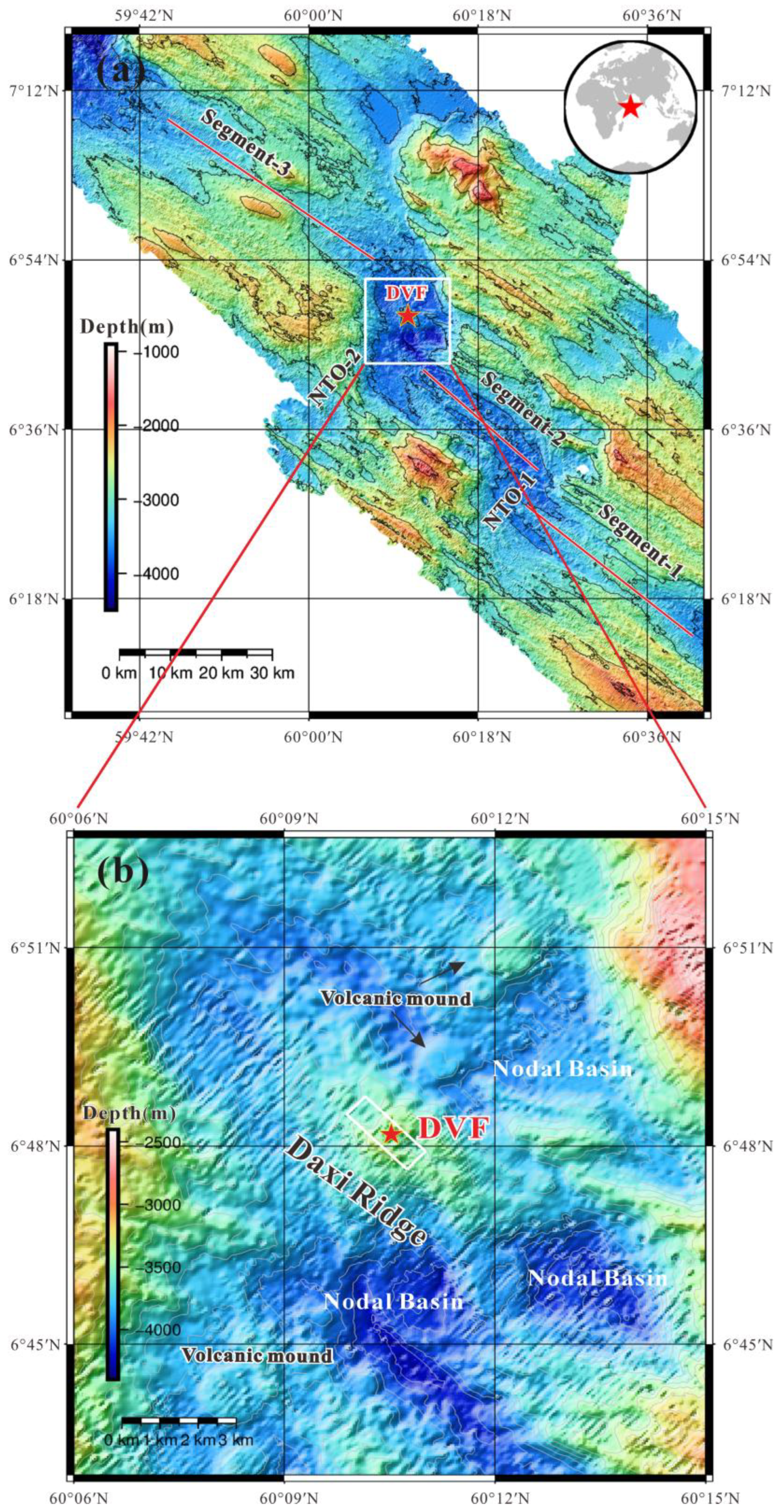
The slow-spreading Carlsberg Ridge is located in the northwestern Indian Ocean, spanning from 2° S to 10° N and 57° E to 60° E, with a total length of approximately 1500 km and a full spreading rate of 22–32 mm/yr [17,18]. The DVF (6°48′ N, 60°10′ E) is situated on a rift valley within a non-transform offset (NTO) zone between two second-order ridge segments with a water depth of ~3500 m (Figure 1). The DVF was first discovered during an investigation of hydrothermal plumes using a towed visual survey system in the Chinese DY33 expedition in 2015 [19]. Investigations revealed three hydrothermal mounds at the DVF. The largest mound, referred to as the Central Mound, is located in the middle, while the other two are named the Northeastern Mound (NE Mound) and the Southwestern Mound (SW Mound) based on their orientations. The Central Mound has a diameter of 180 m, a height of 50 m, and is situated at a depth of approximately 3480 m. Its summit hosts numerous black smoker chimneys, some of which are extinct. The active venting zone spans about 80 m and includes eight chimneys taller than 10 m. The largest active chimney is referred to as “Baochu Pagoda,”. The altered basalt along with brown hydrothermal deposits have been observed on its western flank. The surface of the NE Mound is covered with a layer of brown iron oxide deposits, and an extinct chimney with siliceous material inside has been identified [20]. The SW Mound, approximately 16 m high, is similar in shape and size to the NE Mound. However, as it differs from typical volcanic mounds [21], the SW Mound is inferred to be hydrothermal in origin.

Figure 1.
(a) Bathymetric map of the survey area on the Carlsberg Ridge. (b) Location of the Daxi Vent Field (DVF). The bathymetric data were acquired using multibeam sonar during the Chinese DY24 expedition, with a resolution of 50 m. The white rectangle in panel (b) indicates the range of the near-bottom survey area conducted using the autonomous underwater vehicle (AUV).
3. Data and Methods
3.1. Data Acquisition and Process
In 2019, high-resolution near-bottom magnetic and bathymetric data around the DVF were collected using the “Qianlong III” AUV (Second Institute of Oceanography, Ministry of Natural Resources, Hangzhou, China). “Qianlong III” is a 4500 m-class, untethered, unmanned submersible independently developed by China, measuring approximately 3.5 m in length and weighing about 1.5 tons. It has a maximum speed of 3 knots and can operate continuously for up to 42.8 h. The AUV was programmed to maintain a constant altitude of 100 m above the seafloor, and its attitude (heading, pitch, and roll) was controlled by the onboard inertial navigation system. The bathymetric data were collected using a side-scan sonar mounted on the underside of the AUV. The raw bathymetric data were processed and interpolated into a seafloor terrain grid with a resolution of 1 m. A three-component fluxgate magnetometer was mounted at the stern of the AUV, which continuously acquired high-resolution three-component magnetic data during near-bottom operations and stored them in a self-contained acquisition unit.
The near-bottom magnetic data were first corrected for vehicle-induced magnetic interference to eliminate the effects of the AUV’s magnetic field during measurements. Calibration and correction procedures proposed by Honsho et al. [22] and Bloomer et al. [23] were applied. The magnetic anomaly was then derived by removing the International Geomagnetic Reference Field (IGRF). Considering the short duration of the near-bottom measurement and the fact that the amplitude of the geomagnetic diurnal variation is much smaller than that of the near-bottom magnetic anomaly, we did not perform a diurnal correction. Figure 2 shows the magnetic anomalies.
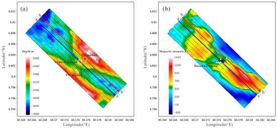
Figure 2.
(a) Near-bottom bathymetric map of the DVF. (b) Near-bottom magnetic anomaly of the DVF. The white triangles in the central part of the map represent inactive hydrothermal vents and the black triangles indicate active hydrothermal vents. The track lines of the AUV are shown in the figure (black solid lines).
3.2. Methods
3.2.1. Magnetic Anomaly Leveling
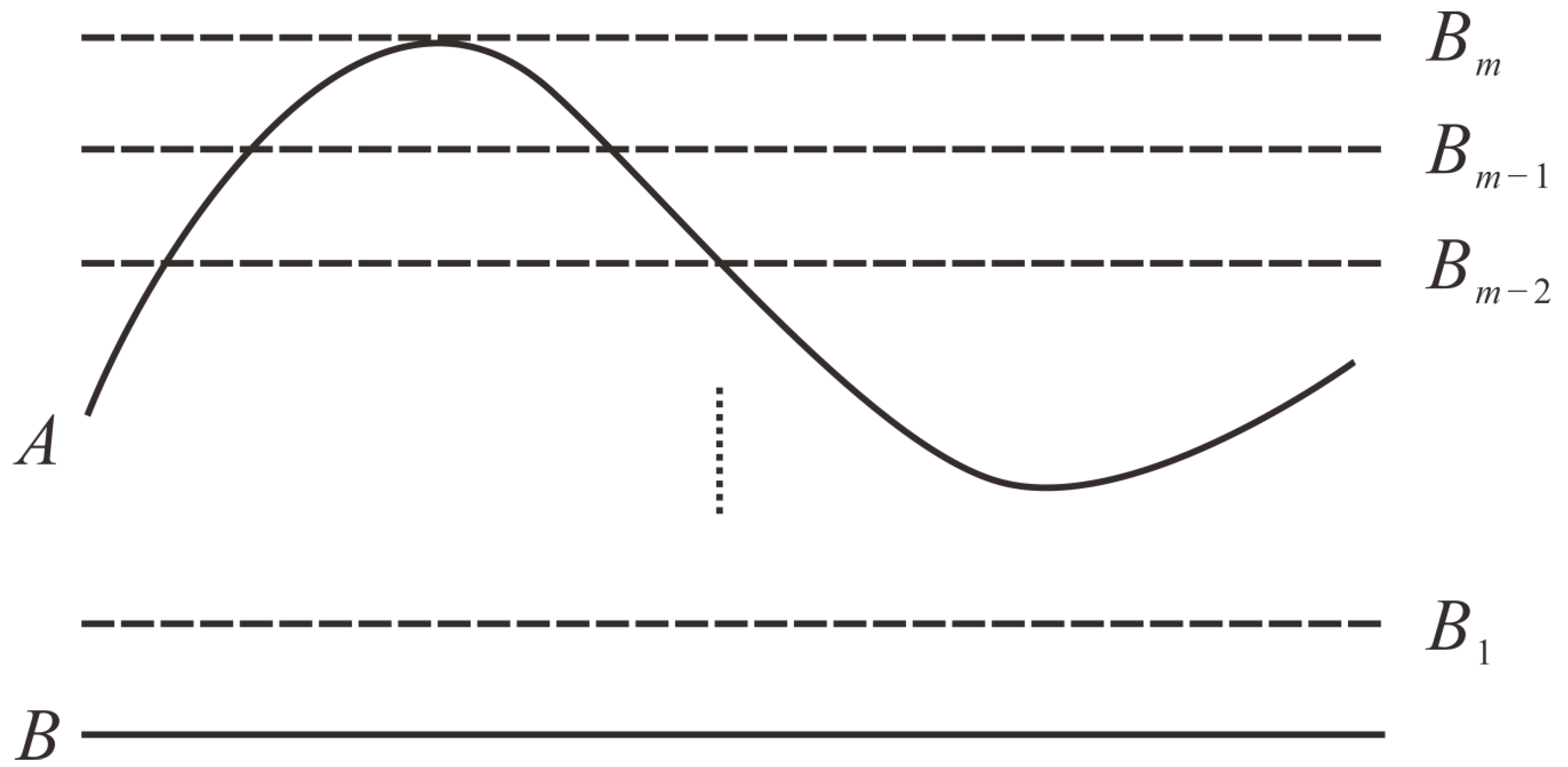
During AUV operations, a terrain-following mode is typically used to maintain a constant altitude above the seafloor, ensuring higher resolution. As a result, the near-bottom magnetic observation surface becomes undulating. However, Fourier transform-based frequency-domain data processing requires the observation surface to be flat. Therefore, we employ the interpolation-iteration method proposed by Xu et al. [24] to level the magnetic anomaly onto a flat surface located 100 m above the highest point of the surveyed terrain profile. The basic procedure of this method is as follows:
- Dividing the space between the top horizontal surface (Bm) and the lower horizontal surface (B) of the undulating observation surface (A) into several equal-spaced sub-surfaces (Bi), as Figure 3 shows;
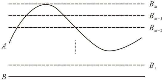 Figure 3. Schematic diagram of the interpolation-iteration leveling method.
 - the magnetic potential field values of the undulating observation surface (A) are projected onto the bottom horizontal surface (B) and used as the initial potential field values of that surface;
- the potential field values of each sub-horizontal surface (Bi) are calculated using frequency-domain upward continuation. These values are interpolated to approximate the potential field of the undulating observation surface (A);
- the residuals between the observed and approximated magnetic anomaly values of the undulating observation surface (A) are calculated and used to correct the magnetic anomaly values on the bottom horizontal surface (B). This process is repeated iteratively until the residuals between the observed and approximated potential field values of the undulating observation surface (A) fall within an acceptable error tolerance.
The magnetic anomaly data from the original observation surface (A) were upward continued in the frequency domain to a leveled reference surface (B), located 100 m above the highest point of the surveyed profile. After 30 iterations of correction, the results indicate that the residuals between the observed and approximated potential field values at the observation surface are less than 5 nT. Therefore, we conclude that the magnetic anomaly values on the leveled profile (B) can be reliably used for the subsequent Euler deconvolution analysis.
3.2.2. Euler Deconvolution
Euler deconvolution can determine the locations of magnetic sources with minimal prior geological information. Based on Euler’s homogeneous equation, this method effectively estimates the positions and depths of magnetic source [25]. The magnetic anomaly data, after being leveled as described in Section 3.2.1, were subjected to two-dimensional Euler deconvolution, and the calculation is expressed as follows:
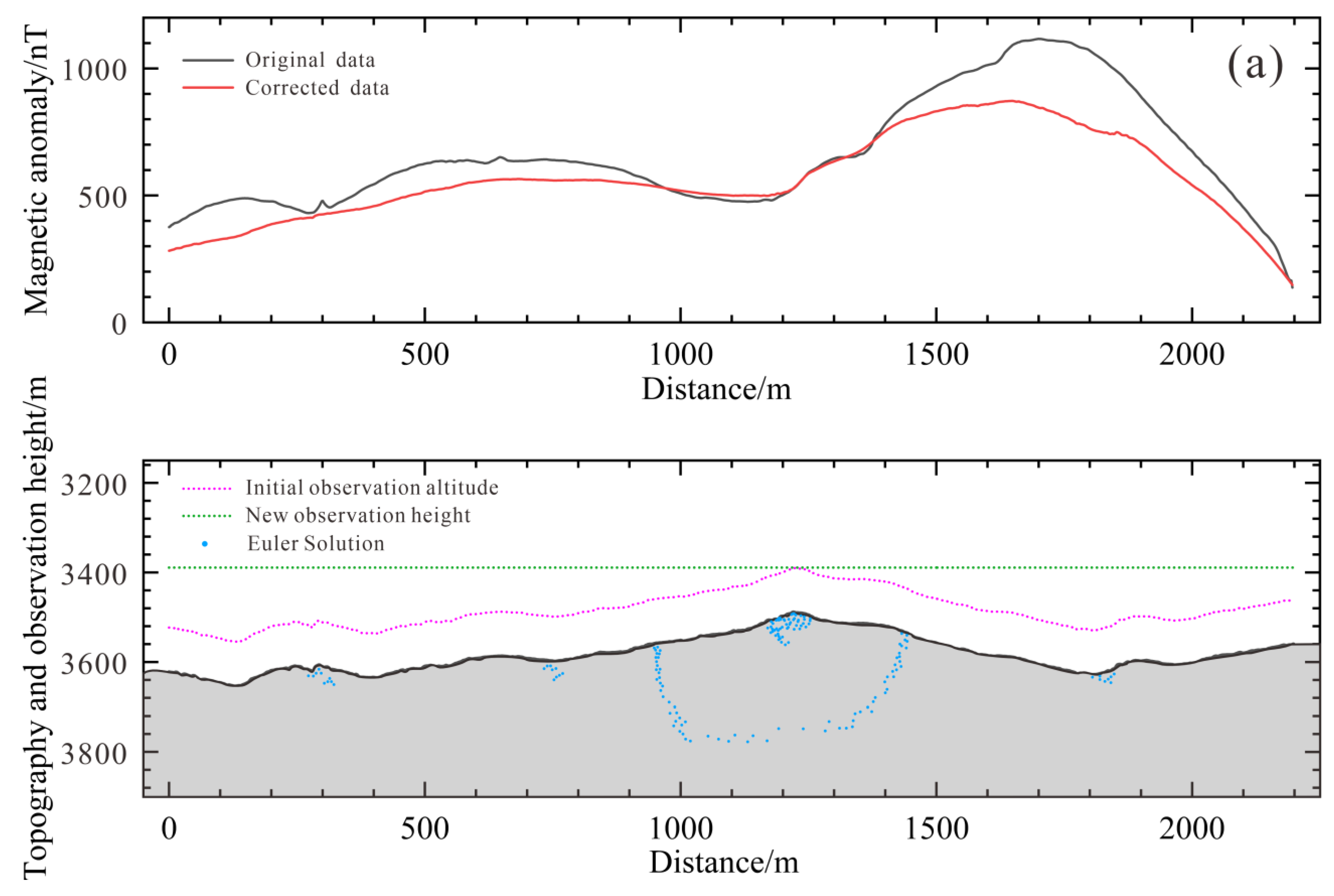
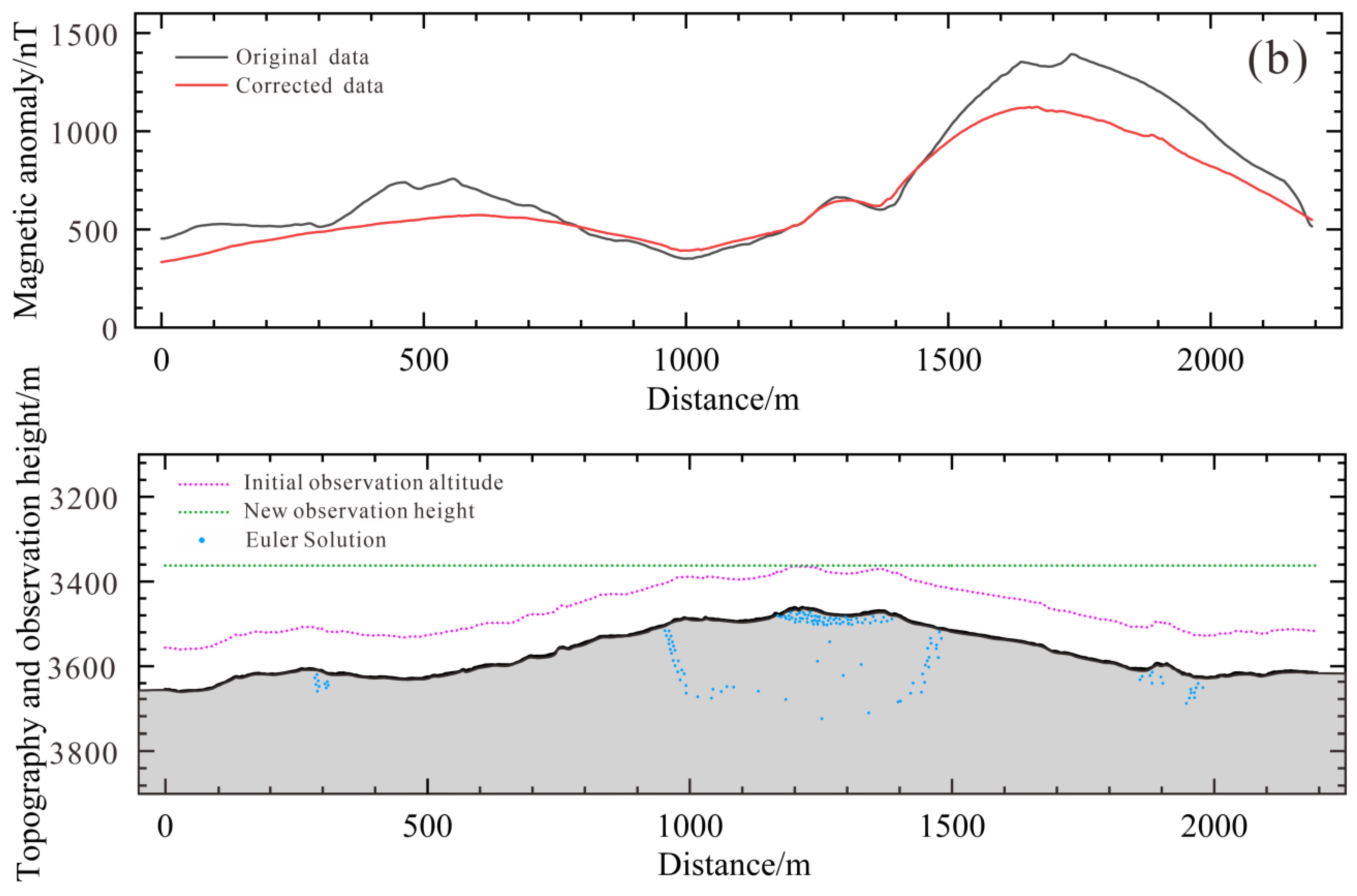
where (x0, z0) are the coordinates of the equivalent source point relative to the profile, and represent the horizontal and vertical derivatives of the magnetic anomaly, respectively, T(x) denotes the magnetic anomaly value, and N is the structural index, set to 1. It is closely related to the geometry of the magnetic bodies in the study area. This index is applicable to tabular structures, sills, and other intrusive geological features. To determine the optimal structural index, multiple tests were conducted using different N values ranging from 0 to 3. The results indicated that when N = 1, the clustering of solutions was most concentrated, making it the optimal structural index. The Euler deconvolution method typically employs a moving window approach to obtain inversion results, where the window size must balance the trade-off between exploration depth, data resolution, and numerical stability. Reid et al. [26] suggested that an optimal inversion performance can be achieved when the window size is 5 to 10 times the grid spacing. For this study area, considering the spectral characteristics of the magnetic anomaly field and the spatial scale of the survey region, a window size of 58 m was selected to obtain the most reliable Euler solutions. Finally, the overdetermined system of equations was solved using the least-squares method to obtain the Euler solutions, whose inversion results provide location information that can be used to delineate the boundaries of different subsurface magnetic bodies. Figure 4 shows the Euler solutions and leveling results.
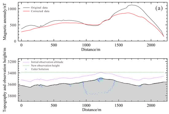
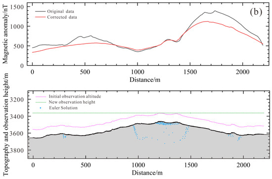
Figure 4.
(a) Leveling results across the active hydrothermal vent of the Central Mound; (b) leveling results across the inactive hydrothermal vent of the NE Mound. The Euler solutions are indicated in the figure.
3.2.3. Magnetic Forward Modeling
There are two magnetic anomaly profiles, aa′ and bb′, across the Central Mound and NE Mound of the DVF, respectively (Figure 2). Using the boundaries inferred from the Euler solutions along profiles aa′ and bb′ as constraints, two initial geological models were constructed. The magnetic forward modeling process begins with constructing a geological model and calculating the magnetic response, which is then compared with the observed data. Semi-automated trial-and-error and error approximation methods are subsequently applied to refine the magnetic structure of the model, achieving optimal agreement between the modeled magnetic anomaly and the observed data [15,16,27].
Before forward modeling, the following assumptions were made: (a) The geomagnetic inclination of the model is assumed to be consistent with the Earth’s magnetic inclination. In other words, the remanent magnetization is considered partially to be superimposed on the induced magnetization. Consequently, the assigned susceptibility values differ from the actual measured magnetic susceptibility of the rock samples and are used solely to represent the correspondence between geological bodies and their magnetic intensity. (b) The magnetic susceptibility within each calculation block is assumed to be uniform.
Based on the IGRF model, the parameters for calculating magnetic anomalies along the survey lines were set as follows: geomagnetic field intensity, 38,009 nT; magnetic declination, −1.701°; magnetic inclination, 0.179°; and survey line azimuth, 135°.
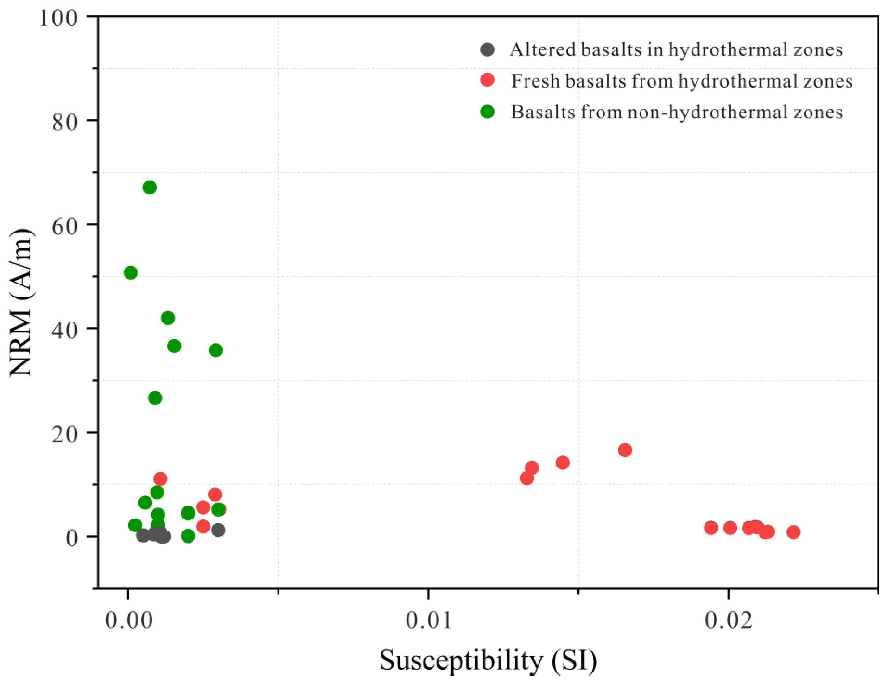
We compiled magnetic susceptibility and natural remanent magnetization (NRM) from basalt samples collected from the Rumble III hydrothermal field on the Kermadec Arc in the Pacific Ocean [28], the Loki’s Castle hydrothermal field on the Mohns Ridge [27], the Southwest Indian Ridge [29], and a non-hydrothermal zone on the Juan de Fuca Ridge [30]. These data were used as references to set our model. Figure 5 shows the compiled rock magnetic parameters. Fresh basalt from hydrothermal zones exhibits higher magnetic susceptibility (red circle). In non-hydrothermal zones, the NRM of basalt varies significantly (green circle), while altered basalts generally display low magnetic susceptibility and a low NRM. The relationships derived from these rock magnetic properties provide constraints for subsequent forward modeling.
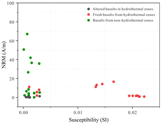
Figure 5.
Magnetic susceptibility and NRM of the basalts from mid-ocean ridge hydrothermal and non-hydrothermal zones.
4. Results and Discussion
The DVF is located on a small, neo-volcanic ridge within a non-transform offset environment. The only comparable geological setting is the Puy de Folles hydrothermal field, located on a large volcanic summit on the Mid-Atlantic Ridge, where a magma chamber is considered to be the heat source driving hydrothermal circulation [31]. Although the location and size of the magma chamber beneath the DVF remains unclear, bathymetric data and towed visual surveys indicate significant magmatic activity beneath the vent field [20].
As Figure 2b shows, the study area of the DVF along the NW–SE direction exhibits high magnetic anomalies at both ends. The southeastern side shows the highest magnetic anomaly, reaching approximately 1400 nT, whereas the northwestern side displays relatively lower anomaly values, ranging from 700 to 900 nT. The active hydrothermal area is located at the center of Figure 2b, where the magnetic anomaly values decrease significantly to a range of 300–500 nT. This low magnetic anomaly zone covers an area of approximately 10,500 m2. A smaller low magnetic anomaly zone is also observed around the extinct hydrothermal vent to the northeast, with anomaly values ranging from 400 to 500 nT, covering an area of approximately 400 m2. The entire study area displays a characteristic pattern of high magnetic anomalies at both ends and low anomalies in the center. The DVF is a basalt-hosted hydrothermal system. Fresh basalts that have not undergone hydrothermal alteration not only retain more of their primary magnetic minerals but also avoid thermal demagnetization and high-temperature oxidation and therefore exhibit higher magnetization intensities. This may be the reason for the high magnetic anomalies observed at both ends of the hydrothermal field.
4.1. The aa′ Profile Cross the Central Mound
Figure 6 shows the aa′ profile. The magnetic anomaly values range from 400 to 1100 nT, displaying a pattern of high anomalies at both ends and lower anomalies in the middle. The Central Mound is the only area in the DVF where hydrothermal venting has been observed. Multiple active chimneys are distributed across its summit, indicating significant hydrothermal activity. A Euler solution cluster appears below the hydrothermal vent, corresponding to the lowest magnetic anomaly zone in the hydrothermal system (Figure 6, yellow area). Towed visual imagery shows fresh hydrothermal sulfides and massive sulfide deposits on the surface. Based on its location, this area is inferred to consist of altered basalt and massive sulfide deposits, extending approximately 120 m along the NW–SE direction with a thickness of 80 m.
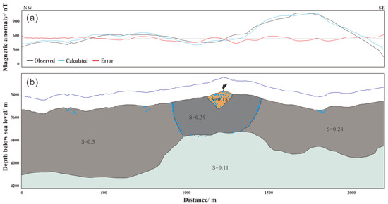
Figure 6.
Forward modeling of magnetic anomalies along profile aa′ (the location shown as the blue line in Figure 2). (a) Observed and calculated magnetic anomalies; (b) magnetic structure and Euler solution distribution. In (b), the blue dots represent Euler solutions, the yellow region denotes altered basalt and massive sulfide deposits, the dark gray region represents fresh basalt from the hydrothermal field, the light gray region indicates basalt from non-hydrothermal areas, and the green region represents gabbro. The blue line represents the observation surface at 100 m above the seafloor. S denotes magnetic susceptibility (SI).
In addition, a notable feature is the “U-shaped” Euler solution cluster surrounding the vent center. The “U-shaped” solution cluster is located at approximately 950 m and 1450 m along the survey line, symmetrically distributed around the hydrothermal vent. On both sides of the ‘U-shaped’ solution cluster the solutions are densely distributed and continuously aligned, whereas at the bottom, they become more scattered, extending to depths of 300 m below the seafloor. Based on magnetic forward modeling results, the “U-shaped” solution cluster is interpreted as representing a basaltic wall. The two sides of the “U-shape” may correspond to the boundaries between basaltic blocks with different magnetic properties. At approximately 300 m and 1800 m of the profile, several shallow Euler solution clusters are observed, which may represent shallow fractures with limited vertical extension.
4.2. The bb′ Profile Cross the NE Mound
Figure 7 shows the bb′ profile. The magnetic anomaly variation is similar to that of the Central Mound, but the anomaly values are higher, ranging from 400 to 1400 nT. Extinct vents have been identified in the NE Mound area, with no signs of hydrothermal activity. The NE Mound represents a hydrothermal deposit formed after a complete cycle of hydrothermal activity, and the geological bodies within the deposit are no longer active. The Euler solution cluster on this profile is mainly concentrated at the top of the mound, spanning approximately 220 m along the NW–SE direction and reaching a thickness of only 30 m. Forward modeling reveals low magnetization in this region. Towed visual surveys show hydroxide iron deposits on the surface, and mineralogical analysis of extinct chimney interiors indicates abundant siliceous material [20]. This suggests that the region is primarily composed of hydrothermal sulfide deposits and an associated network of vein layers. A “U-shaped” solution cluster also appears in the bb′ profile, with structural orientation, depth, and modeled magnetic susceptibility closely resembling those of the aa′ profile. The smaller Euler solution clusters are also observed at approximately 300 m and 1900 m along the profile, indicating the presence of shallow fractures or faults within the basaltic oceanic crust.
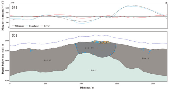
Figure 7.
Forward modeling of magnetic anomalies of the profile bb′ (profile location shown as the red line in Figure 2). (a) Observed and calculated magnetic anomalies; (b) magnetic structure and Euler solution distribution. In (b), the blue dots represent Euler solutions, the yellow region represents hydrothermal sulfide deposits and the network of vein layers, the dark gray region represents fresh basalt from the hydrothermal field, the light gray region indicates basalt from non-hydrothermal areas, and the green region represents gabbro. The blue line represents the observation surface at 100 m above the seafloor. S denotes magnetic susceptibility (SI).
4.3. Structure of the Hydrothermal Field
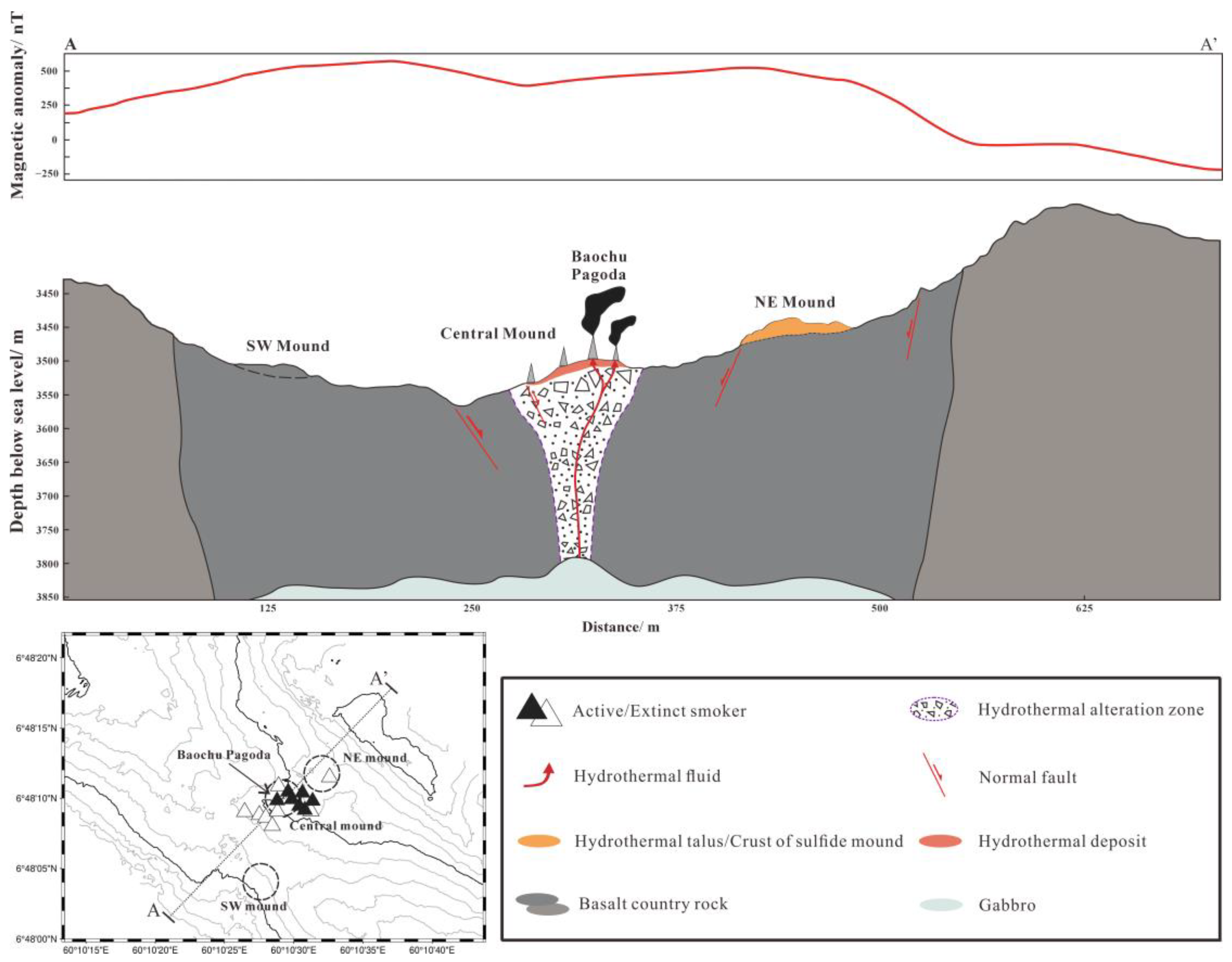
Analysis of the hydrothermal fluid geochemistry at the DVF suggests that the separation of hydrothermal fluids is the primary factor controlling metal enrichment in chimney structures [32]. This indicates a sufficient magmatic heat supply and crustal permeability in the basement, facilitating hydrothermal circulation within the neo-volcanic ridge. This model differs from traditional detachment fault-type seafloor massive sulfide deposits found in NTO systems [33,34]. Based on the fitting results of the aa′ and bb′ magnetic profiles, we constructed a schematic cross-sectional diagram perpendicular to the ridge axis, traversing the Central Mound and NE Mound, along with the corresponding magnetic anomalies (Figure 8). It is evident that the hydrothermal alteration zone at the Central Mound and the hydrothermal deposit at the NE Mound both correspond to magnetic anomaly lows. Small-scale fractures and faults, which are widely present in the DVF, enhance permeability. Even though magmatic supply in NTOs is relatively lower compared to segment centers [35], it remains sufficient to drive high-temperature hydrothermal circulation. This suggests that neo-volcanic ridges within NTOs at slow-spreading centers could be promising targets for hydrothermal area exploration.
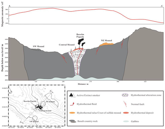
Figure 8.
Schematic cross-sectional diagram traversing both the Central Mound and NE Mound. The SW Mound, not directly intersected by the profile, is projected onto this plane.
5. Conclusions
Using near-bottom bathymetric and magnetic survey data collected by AUV at the Daxi Vent Field, located within a non-transform offset zone on the slow-spreading Carlsberg Ridge, we performed leveling and Euler deconvolution on magnetic profiles across the Central Mound and NE Mound. The boundaries of magnetic source bodies indicated by the Euler solutions were used as constraints for 2.5D forward modeling of the two magnetic profiles. The results indicate that the hydrothermal alteration zone at the active Central Mound extends approximately 120 m along the NW–SE direction, with a depth of about 80 m, while the hydrothermal deposit at the inactive NE Mound extends up to 220 m with a thickness of about 30 m. Fractures and faults are widely developed in the Daxi Vent Field, providing fluid pathways for seawater to penetrate deeper and participate in the hydrothermal circulation.
Author Contributions
Conceptualization, Z.W. and X.H.; Methodology, Z.W. and X.H.; Validation, Z.W., X.H., Y.W. and J.Z.; Formal analysis, Z.W. and X.H.; Investigation, Z.W., X.H. and Y.W.; Resources, Z.W. and X.H.; Data curation, Z.W. and X.H.; Writing—original draft, P.Z.; Writing—review & editing, P.Z., Z.W., X.H., J.Z. and Q.W.; Supervision, Z.W. and X.H.; Project administration, Z.W. and X.H.; Funding acquisition, Z.W. and X.H. All authors have read and agreed to the published version of the manuscript.
Funding
This research was funded by the National Key Research and Development Program of China (No. 2021YFF0501301), National Natural Science Foundation of China (Nos. 42076078, 42172231).
Institutional Review Board Statement
Not applicable.
Informed Consent Statement
Not applicable.
Data Availability Statement
Data are contained within the article.
Conflicts of Interest
The authors declare no conflict of interest.
References
- Rona, P.A. Resources of the Sea Floor. Science 2003, 299, 673–674. [Google Scholar] [CrossRef]
- Cathles, L.M. What processes at mid-ocean ridges tell us about volcanogenic massive sulfide deposits. Min. Depos. 2011, 46, 639–657. [Google Scholar] [CrossRef]
- Rona, P.A. Criteria for recognition of hydrothermal mineral deposits in oceanic crust. Econ. Geol. 1978, 73, 135–160. [Google Scholar] [CrossRef]
- Kent, D.V.; Gee, J. Magnetic alteration of zero-age oceanic basalt. Geology 1996, 24, 703–706. [Google Scholar] [CrossRef]
- de Ronde, C.E.J.; Hannington, M.D.; Stoffers, P.; Wright, I.C.; Ditchburn, R.G.; Reyes, A.G.; Baker, E.T.; Massoth, G.J.; Lupton, J.E.; Walker, S.L.; et al. Evolution of a Submarine Magmatic-Hydrothermal System: Brothers Volcano, Southern Kermadec Arc, New Zealand. Soc. Econ. Geol. 2005, 100, 1097–1133. [Google Scholar] [CrossRef]
- Szitkar, F.; Dyment, J.; Choi, Y.; Fouquet, Y. What causes low magnetization at basalt-hosted hydrothermal sites? Insights from inactive site Krasnov (MAR 16°38′ N). Geochem. Geophys. Geosyst. 2014, 15, 1441–1451. [Google Scholar] [CrossRef]
- Dyment, J.; Tamaki, K.; Horen, H.; Fouquet, Y.; Nakase, K.; Yamamoto, M.; Ravilly, M.; Kitazawa, M. A Positive Magnetic Anomaly at Rainbow Hydrothermal Site in Ultramafic Environment. Am. Geophys. Union 2005, 2005, OS21C-08. [Google Scholar]
- Charlou, J.L.; Donval, J.P.; Konn, C.; Ondréas, H.; Fouquet, Y.; Jean-Baptiste, P.; Fourré, E. High production and fluxes of H2 and CH4 and evidence of abiotic hydrocarbon synthesis by serpentinization in ultramafic-hosted hydrothermal systems on the Mid-Atlantic Ridge. Geophys. Monogr. Ser. 2010, 188, 265–296. [Google Scholar]
- Wu, T.; Tao, C.; Liu, C.; Li, H.; Wu, Z.; Wang, S.; Chen, Q. Geomagnetic Models and Edge Recognition of Hydrothermal Sulfide Deposits at Mid-ocean Ridges. Mar. Georesour. Geotecnol. 2015, 34, 630–637. [Google Scholar] [CrossRef]
- Tontini, F.C.; Davy, B.; De Ronde, C.E.J.; Embley, R.W.; Leybourne, M.; Tivey, M.A. Crustal magnetization of Brothers Volcano, New Zealand, measured by autonomous underwater vehicles; geophysical expression of a submarine hydrothermal system. Econ. Geol. Bull. Soc. Econ. Geol. 2012, 107, 1571–1581. [Google Scholar] [CrossRef]
- Tontini, F.C.; Crone, T.J.; de Ronde, C.E.J.; Fornari, D.J.; Kinsey, J.C.; Mittelstaedt, E.; Tivey, M. Crustal magnetization and the subseafloor structure of the ASHES vent field, Axial Seamount, Juan de Fuca Ridge; implications for the investigation of hydrothermal sites. Geophys. Res. Lett. 2016, 43, 6205–6211. [Google Scholar] [CrossRef]
- Cocchi, L.; Tontini, F.C.; Muccini, F.; de Ronde, C.E.J. Magnetic Expression of Hydrothermal Systems Hosted by Submarine Calderas in Subduction Settings: Examples from the Palinuro and Brothers Volcanoes. Geosciences 2021, 11, 504. [Google Scholar] [CrossRef]
- Szitkar, F.; Dyment, J.; Fouquet, Y.; Choi, Y.; Honsho, C. Absolute magnetization of the seafloor at a basalt-hosted hydrothermal site: Insights from a deep-sea submersible survey. Geophys. Res. Lett. 2015, 42, 1046–1052. [Google Scholar] [CrossRef]
- Tivey, M.A.; Rona, P.A.; Schouten, H. Reduced crustal magnetization beneath the active sulfide mound, TAG hydrothermal field, Mid-Atlantic Ridge at 26° N. Earth Planet. Sci. Lett. 1993, 115, 101–115. [Google Scholar] [CrossRef]
- Talwani, M.; Heirtzler, J.R. Computation of magnetic anomalies caused by two dimensional structures of arbitary shape. Comput. Miner. Ind. 1964, 1, 464–480. [Google Scholar]
- Rasmussen, R.; Pedersen, L.B. End corrections in potential field modeling. Geophys. Prospect. 1979, 27, 749–760. [Google Scholar] [CrossRef]
- Raju, K.K.; Chaubey, A.; Amarnath, D.; Mudholkar, A. Morphotectonics of the Carlsberg Ridge between 62°20′ and 66°20′ E, northwest Indian Ocean. Mar. Geol. 2008, 252, 120–128. [Google Scholar] [CrossRef]
- Han, X.; Wu, Z.; Qiu, B. Morphotectonic characteristics of the northern part of the Carlsberg Ridge near the Owen Fracture Zone and the occurrence of oceanic core complex formation. AGU Fall Meet. Abstr. 2012, 2012, OS13B-1722. [Google Scholar]
- Jiang, Z.; Han, X.; Wang, Y.; Qiu, Z. Characteristics of water chemistry and constituents of particles in the hydrothermal plume near 6°48′ N, Carlsberg Ridge, Northwest Indian Ocean. J. Mar. Sci. 2017, 35, 34–43. [Google Scholar] [CrossRef]
- Wang, Y.; Han, X.; Zhou, Y.; Qiu, Z.; Yu, X.; Petersen, S.; Li, H.; Yang, M.; Chen, Y.; Liu, J.; et al. The Daxi Vent Field: An active mafic-hosted hydrothermal system at a non-transform offset on the slow-spreading Carlsberg Ridge, 6°48′ N. Ore Geol. Rev. 2021, 129, 103888. [Google Scholar] [CrossRef]
- Jamieson, J.W.; Clague, D.A.; Hannington, M.D. Hydrothermal sulfide accumulation along the Endeavour Segment, Juan de Fuca Ridge. Earth Planet. Sci. Lett. 2014, 395, 136–148. [Google Scholar] [CrossRef]
- Honsho, C.; Ura, T.; Kim, K. Deep-sea magnetic vector anomalies over the Hakurei hydrothermal field and the Bayonnaise knoll caldera, Izu-Ogasawara arc, Japan. J. Geophys. Res. Solid Earth 2013, 118, 5147–5164. [Google Scholar] [CrossRef]
- Bloomer, S.; Kowalczyk, P.; Williams, J.; Wass, T.; Enmoto, K. Compensation of magnetic data for autonomous underwater vehicle mapping surveys. In Proceedings of the 2014 IEEE/OES Autonomous Underwater Vehicles (AUV), Oxford, MS, USA, 6–9 October 2014. [Google Scholar]
- Xu, S.; Yu, H. The Interpolation-Iteration Method for Potential Field Continuation from Undulating Surface to Plane. Chin. J. Geophys. 2007, 50, 1566–1570. [Google Scholar] [CrossRef]
- Reid, A.B.; Allsop, J.M.; Granser, H.; Millett, A.J.; Somerton, I.W. Magnetic interpretation in three dimensions using Euler deconvolution. Geophysics 1990, 55, 80–91. [Google Scholar] [CrossRef]
- Reid, A.B.; Ebbing, J.; Webb, S.J. Avoidable Euler Errors—The use and abuse of Euler deconvolution applied to potential fields. Geophys. Prospect. 2014, 62, 1162–1168. [Google Scholar] [CrossRef]
- Lim, A.; Brönner, M.; Johansen, S.E.; Dumais, M. Hydrothermal Activity at the Ultraslow-Spreading Mohns Ridge: New Insights From Near-Seafloor Magnetics. Geochem. Geophys. Geosyst. 2019, 20, 5691–5709. [Google Scholar] [CrossRef]
- Tontini, F.C.; de Ronde, C.E.J.; Kinsey, J.C.; Soule, A.; Yoerger, D.; Cocchi, L. Geophysical modeling of collapse-prone zones at Rumble III seamount, southern Pacific Ocean, New Zealand. Geochem. Geophys. Geosyst. 2013, 14, 4667–4680. [Google Scholar] [CrossRef]
- Bronner, A.; Sauter, D.; Munschy, M.; Carlut, J.; Searle, R.; Cannat, M.; Manatschal, G. Magnetic signature of large exhumed mantle domains of the Southwest Indian Ridge—Results from a deep-tow geophysical survey over 0 to 11 Ma old seafloor. Solid Earth 2014, 5, 339–354. [Google Scholar] [CrossRef]
- Johnson, H.P.; Tivey, M.A. Magnetic properties of zero-age oceanic crust; a new submarine lava flow on the Juan de Fuca Ridge. Geophys. Res. Lett. 1995, 22, 175–178. [Google Scholar] [CrossRef]
- Cherkashov, G.; Poroshina, I.; Stepanova, T.; Ivanov, V.; Bel’Tenev, V.; Lazareva, L.; Rozhdestvenskaya, I.; Samovarov, M.; Shilov, V.; Glasby, G.P.; et al. Seafloor massive sulfides from the northern equatorial Mid-Atlantic Ridge; new discoveries and perspectives. Mar. Georesour. Geotechnol. 2010, 28, 222–239. [Google Scholar] [CrossRef]
- Wu, X.; Han, X.; Wang, Y.; Garbe-Schönberg, D.; Schmidt, M.; Zhang, Z.; Qiu, Z.; Zong, T.; Zhou, P.; Yu, X.; et al. Geochemistry of vent fluids from the Daxi Vent Field, Carlsberg Ridge, Indian Ocean: Constraints on subseafloor processes beneath a non-transform offset. Mar. Geol. 2023, 455, 106955. [Google Scholar] [CrossRef]
- Canales, J.P.; Dunn, R.A.; Arai, R.; Sohn, R.A. Seismic imaging of magma sills beneath an ultramafic-hosted hydrothermal system. Geology 2017, 45, 451–454. [Google Scholar] [CrossRef]
- Melchert, B.; Devey, C.; German, C.; Lackschewitz, K.; Seifert, R.; Walter, M.; Mertens, C.; Yoerger, D.; Baker, E.; Paulick, H.; et al. First evidence for high-temperature off-axis venting of deep crustal/mantle heat: The Nibelungen hydrothermal field, southern Mid-Atlantic Ridge. Earth Planet. Sci. Lett. 2008, 275, 61–69. [Google Scholar] [CrossRef]
- Tivey, M.A.; Dyment, J. The magnetic signature of hydrothermal systems in slow spreading environments. In Diversity of Hydrothermal Systems on Slow Spreading Ocean Ridges; Rona, P.A., Devey, C.W., Dyment, J., Murton, B.J., Eds.; American Geophysical Union: Washington, DC, USA, 2010; Volume 188, pp. 43–66. [Google Scholar] [CrossRef]


Disclaimer/Publisher’s Note: The statements, opinions and data contained in all publications are solely those of the individual author(s) and contributor(s) and not of MDPI and/or the editor(s). MDPI and/or the editor(s) disclaim responsibility for any injury to people or property resulting from any ideas, methods, instructions or products referred to in the content. |
© 2025 by the authors. Licensee MDPI, Basel, Switzerland. This article is an open access article distributed under the terms and conditions of the Creative Commons Attribution (CC BY) license (https://creativecommons.org/licenses/by/4.0/).