Article

Research on Energy Dissipation Mechanism of Hump Characteristics Based on Entropy Generation and Coupling Excitation Mechanism of Internal Vortex Structure of Waterjet Pump at Hump Region

1
Wuhan Second Ship Design and Research Institute, Wuhan 430064, China
2
National Research Center of Pumps, Jiangsu University, Zhenjiang 212013, China
*
Author to whom correspondence should be addressed.
J. Mar. Sci. Eng. 2025, 13(3), 442; https://doi.org/10.3390/jmse13030442
Submission received: 13 January 2025 / Revised: 18 February 2025 / Accepted: 25 February 2025 / Published: 26 February 2025
(This article belongs to the Section Ocean Engineering)

Abstract

:
High-speed mixed-flow and axial-flow pumps often exhibit hump or double-hump patterns in flow–head curves. Operating in the hump region can cause flow disturbances, increased vibration, and noise in pumps and systems. Variable-speed ship navigation requires waterjet propulsion pumps to adjust speeds. Speed transitions can lead pumps into the hump region, impacting efficient and quiet operation. This paper focuses on mixed-flow waterjet propulsion pumps with guide vanes. Energy, entropy production, and flow characteristic analyses investigate hump formation and internal flow properties. High-speed photography in cavitation experiments focuses on increased vibration and noise in the hump region. This study shows that in hump formation, impeller work capacity decreases less than internal fluid loss in the pump. These factors lead to an abnormal increase in the energy curve. The impeller blades show higher pressure at peak conditions than in valley conditions. Valley conditions show more pressure and velocity distribution variance in impeller flow passages, with notable low-pressure areas. This research aids in understanding pump hump phenomena, addressing flow disturbances, vibration, noise, and supporting design optimization.

1. Introduction

The superior performance of mixed-flow pumps, including high flow capacity, operational efficiency, and resistance to cavitation, makes them a critical component in applications across the shipbuilding, agriculture, water management, and power sectors. [1,2]. Mixed-flow pumps, crucial in ship waterjet propulsion, major water conservancy initiatives, seawater desalination, pumped storage, and nuclear and thermal power plant cooling systems [3], require significant stability [4]. Waterjet propulsion pumps consist of an inlet waterway, a rotating impeller, stationary guide vanes, a contraction nozzle, a pump casing, and a shaft system, as shown in Figure 1. However, mixed-flow and axial-flow pumps with high specific speeds often display hump or double-hump patterns in their flow–head curves. Operation in the hump region can lead to issues like flow disturbances, increased vibration, and noise in the pump and overall system. As ships change speeds, waterjet propulsion pumps must adjust their rotational speeds to match. During speed transitions, pumps may enter the hump region, adversely affecting efficient and quiet ship operation, crew comfort, and military vessel stealth, potentially damaging the propulsion system.
The flow–head curve is a graph that describes the relationship between the pump head (H) and the flow rate (Q), typically obtained through experiments or numerical simulations. The unusual bend in the flow–head curve, termed the hump characteristic, is illustrated in Figure 2, where the horizontal axis represents QnD, a dimensionless parameter used to characterize the pump’s flow performance. It is typically defined as the ratio of the pump flow rate (Q) to a reference flow rate. The vertical axis represents EnD, a dimensionless parameter used to characterize the pump’s energy performance. It is usually defined as the ratio of the pump head (H) to a reference energy value. This phenomenon’s occurrence area is called the hump characteristics region, or the saddle region by some scholars. Scholars generally agree that the hump characteristics originate from a change in the pump’s flow state. However, two primary theories explain these characteristics: one attributes them to non-monotonic changes in hydraulic losses from varying pump flow states, and the other to changes in the impeller’s work capacity due to internal flow alterations. In centrifugal pumps, the performance stability correlates with the flow–head curve’s slope [5]: a larger absolute slope value indicates increased stability in the performance curve.
Long Yun and colleagues [6] propose that cavitation vortices, extending and fracturing between blades, decrease waterjet propulsion pump efficiency. Furthermore, cavitation on the pressure surface can obstruct flow passages, leading to flow separation and reduced pump head [7]. This leads to significant energy loss [8], deterioration of the internal flow field, increased flow-induced noise, and can even threaten the rotor blades’ service life, potentially damaging the impeller blades [9]. Weixiang Ye et al. [10] attribute the hump characteristics to a notable increase in energy losses within the mixed-flow pump impeller, significantly reducing blade loading near the leading edge, resulting in a head drop. Yang Jun et al., G Pavesi et al., Uroš Ješe et al., and O Braun et al. [11,12,13,14,15] assert that the dynamic and static interactions between the impeller and guide vanes, affecting flow structure and pressure pulsations, contribute to hump characteristics in the flow–head curve under pump conditions. Figure 3 shows a schematic representation of the effect of the hump region on the hydrodynamic performance of the pump.
This paper explores the causes of hump characteristics in mixed-flow waterjet propulsion pumps. Utilizing numerical simulations, this paper employs energy characteristic curve analysis, entropy production analysis, and flow characteristic analysis. It investigates the impeller’s work capacity, internal flow losses, and pump flow characteristics, uncovering how changes in impeller work capacity and internal flow losses contribute to hump characteristics formation.

2. Hydraulic Performance Testing and Numerical Simulation Methods

2.1. Pump Design Parameters

This experiment examines a mixed-flow waterjet propulsion pump with contraction guide vanes. The model pump features a 250 mm impeller inlet diameter, with its key design and structural parameters detailed in Table 1. Figure 4 depicts the main components of this experimental model pump.

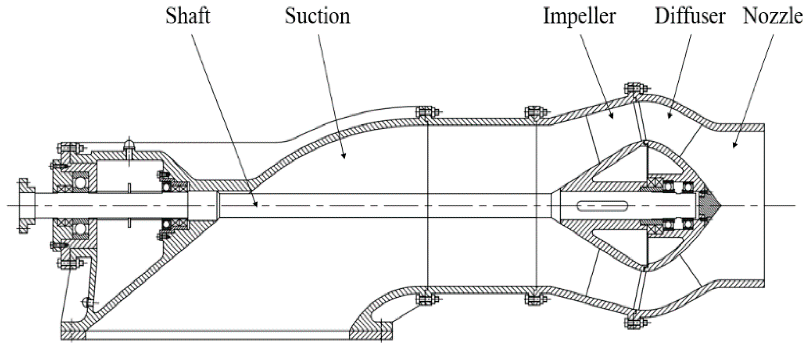
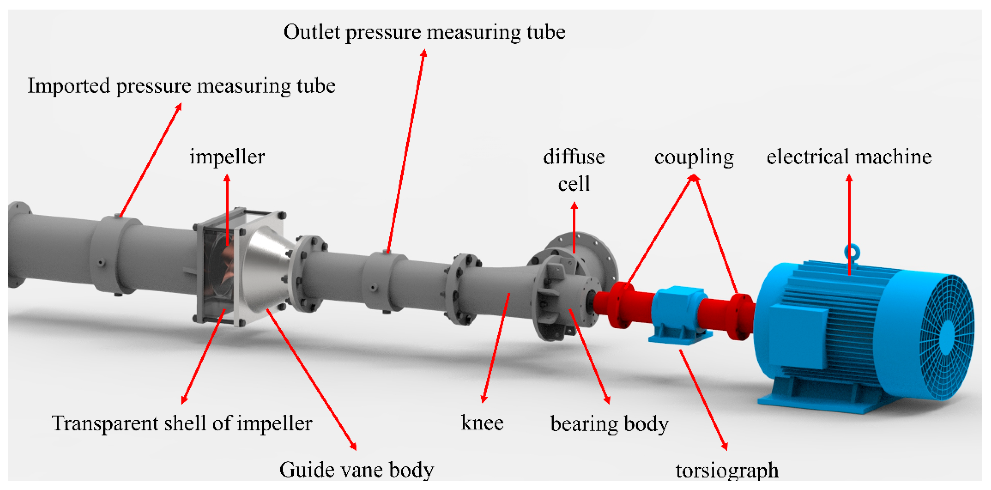
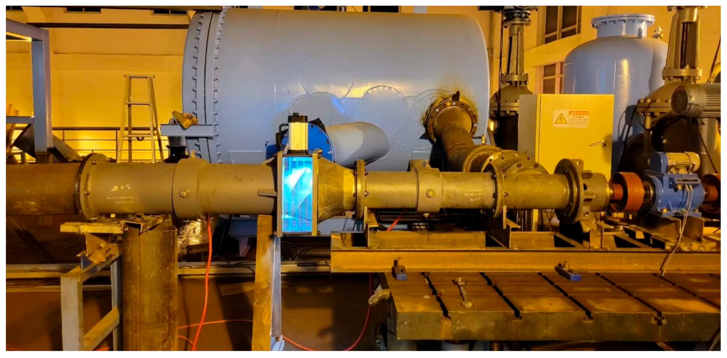
2.2. Structure and Parameters of the Test Pump

2.2.1. The Pressure Distribution Inside the Pump

The experiment was conducted on a closed test bench for axial (mixed) flow pumps at the National Research Center of Pumps, Jiangsu University, as previously utilized by our team in earlier studies [20]. As shown in the Figure 5, this setup included key components like a cavitation tank, vacuum pump, inlet valves, test pump section, and high-speed photography apparatus, among others. The testing system, developed by Jiangsu University’s TPA Research Center, provides precision measurements with an accuracy of 0.2% for power, 0.02% for flow rate, and 0.02% for pressure.

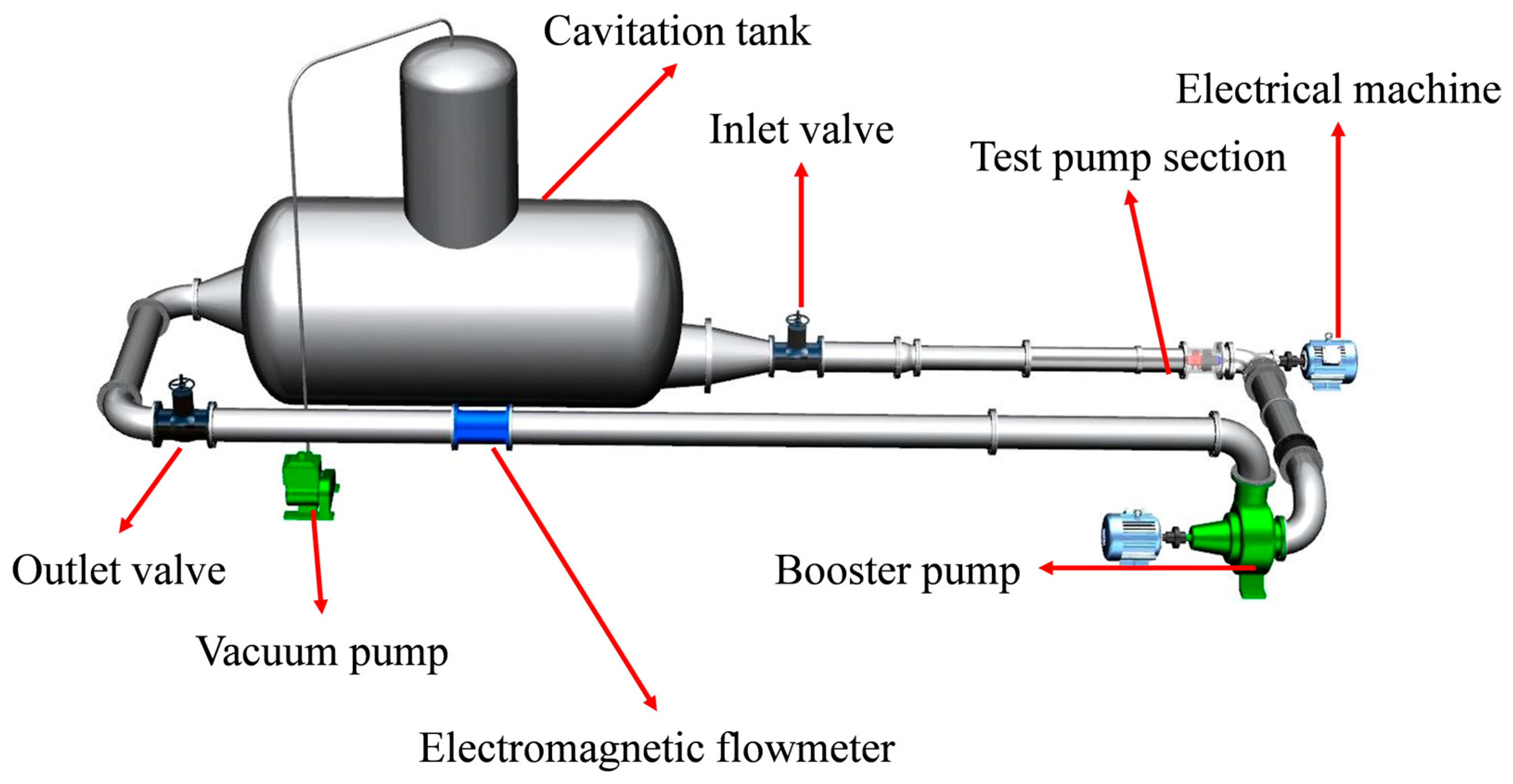
2.2.2. Test Principle and Method

Pressure measurements were made using instrument pressure transducers that converted pressure signals into electrical currents for the pump parameter measuring instrument. Pressure measurement points were positioned at two pipe diameters before the inlet flange and after the outlet flange, ensuring an outlet straight pipe length of at least four pipe diameters. Prior to testing, the pipeline was assembled as shown in Figure 6. The experimental setup is shown in Figure 7. Prior to filling the pipeline with water, a no-load calibration and zero adjustment of the torque meter were performed. The calibration coefficients at different speeds were recorded. During tests at varying speeds, the specific calibration coefficient was input into the torque meter control instrument to counteract mechanical losses from bearings and sealing components. All data were collected to complete the hydraulic performance test.

2.3. Experimental Study on Hydraulic Performance

The flow rates were adjusted and the corresponding test data were collected to complete the pump performance test at different speeds. To enhance the universality of the test results, the test data for flow rate (Q), head (H), and impeller torque (T) were dimensionless, transformed according to the International Electrotechnical Commission (IEC) as follows:
Q nD = Q n D 3
E nD = g H n 2 D 2
T nD = T ρ n 2 D 5
In the formulae, the flow coefficient QnD, the energy coefficient EnD, and the torque coefficient TnD are all dimensionless numbers, and the unit of flow Q is m3/s. The unit of rotation speed n is r/min; the unit of nominal diameter D of the impeller is m; the unit of head H is m; the unit of gravity acceleration g is m/s2; the unit of density ρ is kg/m3; and the unit of torque T is N·m.

2.4. Numerical Simulation Method of Hump Characteristics

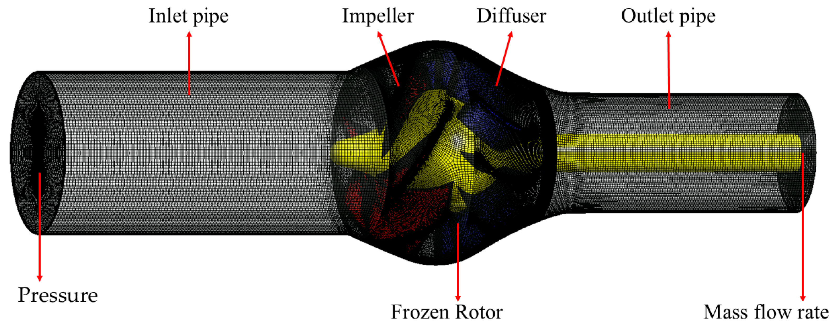
2.4.1. Computational Fluid Domain

This study examined a mixed-flow waterjet propulsion pump equipped with adjustable guide vanes. The commercial computational software ANSYS CFX 2021 R1 simulates the areas before the inlet and after the outlet as infinitely long straight pipes. Previous studies have shown minimal differences between the results obtained using elbow and straight pipe inflow configurations. Therefore, to conserve computational resources, this study utilized a straight pipe inflow approach for subsequent calculations [21]. Figure 8 displays the results of both numerical modeling approaches after dimensionless conversion.

2.4.2. Mesh Subdivision

TurboGrid generated hexahedral structured meshes for the impeller and guide vane fluid domains. Straight pipe sections were incorporated at the impeller inlet and the guide vane outlet. ICEM CFD was used to generate the hexahedral structured mesh. Figure 9 shows the overall computational mesh, and Figure 10 illustrates the local mesh of the hydraulic components. Boundary layer refinement was applied to all meshes, with the wall surface Y+ values for each component detailed in Table 2. This configuration ensures that the first mesh layer lies within the viscous sublayer, conforming to the requirements of the SST k-ω turbulence model.

2.4.3. Boundary Conditions

Hydraulic performance calculations for the model pump were conducted using ANSYS CFX 2021 R1. Simulations assumed the liquid phase as water at 25 °C, using default material properties from the software’s library. The SST k-ω model was employed as the turbulence model. The impeller fluid domain was designated as rotating, with varying speeds, as per calculation requirements, while other fluid domains remained stationary. The detailed settings are shown in Table 3.

2.4.4. Grid Independence Verification

Our team has finished the grid independence verification in previous research [22], as shown in Figure 11. Finally, Scheme 5 was selected for its finer resolution of the flow field structure, comprising around 12.54 million grids in total.

3. Hump Characteristics Analysis

The prevalent view identifies two key factors contributing to the hump phenomenon in pump flow–head curves. These factors are variations in impeller performance and changes in internal flow losses. Yet, a unified consensus on the hump effect’s extent across different pump types remains elusive. This chapter employs numerical simulations to explore the hump phenomenon’s causes in mixed-flow jet propulsion pumps. This study uses energy characteristic curve analysis, entropy production analysis, and flow characteristic analysis to examine how impeller performance changes and internal flow losses influence hump formation.

3.1. Hump Characteristics Analysis Method

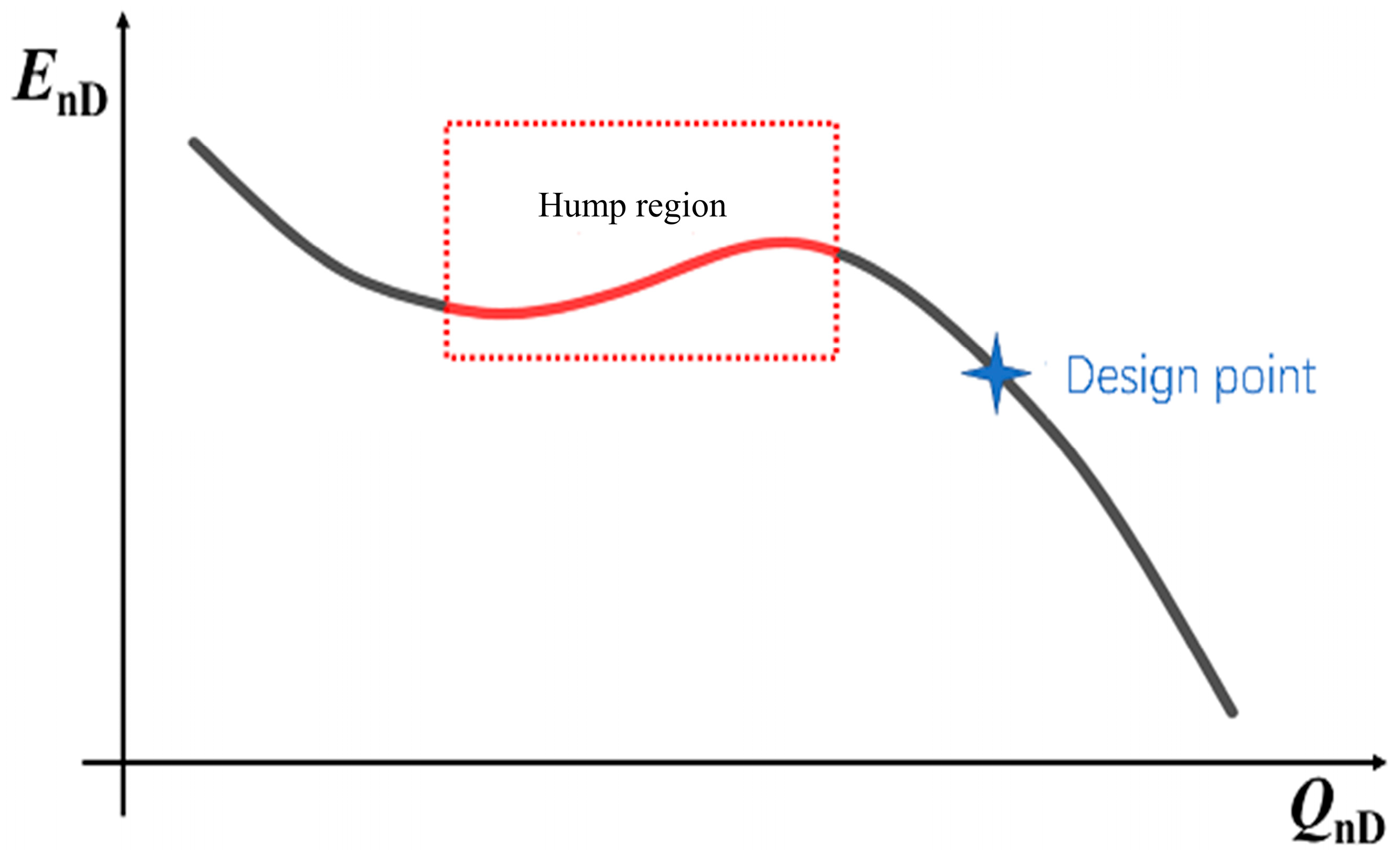
3.1.1. Energy Characteristic Curve Analysis Method

The theoretical energy coefficient Et, the energy coefficient EnD, and the hydraulic loss energy coefficient Eloss can all be considered as functions of the flow coefficient QnD. To simplify the expressions, EnD (QnD), Et (QnD), and Eloss (QnD) will be abbreviated as EnD, Et, and Eloss, respectively, in the following discussion. Given that Eloss is defined as a negative value, the following relationship exists among these energy coefficients:
E nD Q nD = E t Q nD + E loss Q nD
E loss = k = 1 4 E loss - k
In the equation, the value of k is taken as 1, 2, 3, and 4, which correspond to the inlet pipe, impeller, guide vane, and outlet pipe, respectively.
The variation trend of the energy characteristic curve can be represented by the slope:
k E nD = d E nD d Q nD
k E t = d E t d Q nD
k E loss = d E loss d Q nD
k E nD = k E t + k E loss
k E loss = k = 1 4 d E loss - k d Q nD
Since the data can only be obtained at different flow coefficient operating points during experiments or numerical simulations, the hydraulic performance curve consists of discrete points. Therefore, the above equations need to be discretized as follows:
k e = e i + 1 e i ( Q nD ) i + 1 ( Q nD ) i
In this equation, e represents the factors EnD, Et, and Eloss, while k(e) represents the slope of the corresponding curve for factor e.
Equation (6) indicates that the slope of the EnD curve equals the slope of the Et curve plus the sum of the slopes of the hydraulic loss energy coefficient Eloss curves for all components. When the slope of the EnD curve is negative, the energy characteristic curve does not exhibit a hump. However, when the slope of the EnD curve changes from negative to positive, the energy characteristic curve develops a hump.
By determining the sign of k(EnD), we can assess whether a hump phenomenon will occur in the energy characteristic curve. That is, by comparing the sign of k(Et) with the sum of k(Eloss), we can predict the emergence of the hump. In other words, the hump phenomenon is caused by the transition of k(EnD) from negative to positive, which is related to the changes in k(Et) and k(Eloss).
Taking the derivative of Equation (6) with respect to QnD yields:
d d Q nD d E nD d Q nD = d d Q nD d E t d Q nD + d d Q nD d E loss d Q nD
Equation (9) indicates that the change in the slope of the EnD curve is equal to the sum of the changes in the slopes of the Et curve and the Eloss curve. By solving the second derivatives of Et and Eloss, we can quantitatively assess the contribution of their variations to the formation of the hump.
To better describe the changes in the slopes of the energy coefficient curves, the concept of “Deflection Degree” (Df) is introduced, which is expressed as follows:
D f E nD = d d Q nD d E nD d Q nD
D f E t = d d Q nD d E t d Q nD
D f E loss - k = d d Q nD d E loss - k d Q nD
D f E loss = d d Q nD k = 1 4 d E loss - k d Q nD = k = 1 4 D f E loss - k
D f E nD = D f E t + D f E loss = D f E t + k = 1 4 D f E loss - k
Similarly, the above equations undergo the following discretization process:
D f e = e i + 1 e i ( Q nD ) i + 1 ( Q nD ) i e i e i - 1 ( Q nD ) i ( Q nD ) i - 1 ( Q nD ) i + 1 ( Q nD ) i
In the equation, Df(e) represents the change in the slope of the curve corresponding to factor e, i.e., the degree of deflection of the curve. The larger the absolute value of Df(e) at a certain flow rate condition, the greater the deflection of the corresponding factor e curve at that condition.
The deflection degree Df(e) can assess the degree of deflection of the curve corresponding to factor e at a specific flow rate condition, but it does not directly reflect the contribution of factor e to the deflection of the EnD energy characteristic curve. To address this, the concept of “Deflection Contribution Factor” (Cf) is introduced, which is expressed as follows:
C f E t = D f E t D f E nD
C f E loss = D f E loss D f E nD
C f E t + C f E loss = 1
In other words, at a certain flow rate condition, the deflection contribution factor Cf(e) for factor e is equal to the ratio of the deflection degree Df(e) of that factor to the deflection degree Df(end) of the energy coefficient. The magnitude of this ratio represents the contribution of factor e to the deflection of the EnD energy characteristic curve at a specific flow rate condition, or in other words, the contribution of factor e to the formation of the hump in the EnD energy characteristic curve at that flow rate condition.

3.1.2. Entropy Generation Analysis Method

According to the second law of thermodynamics, the dissipation caused by irreversible factors in an irreversible process is called entropy generation, and entropy generation is always positive. During the operation of the waterjet pump, undesirable flow conditions such as backflow, vortices, and flow separation lead to irreversible energy dissipation. The entropy generation analysis method can be used to locate and assess energy dissipation within the waterjet pump. The energy dissipation forms in the pump can be divided into five types: direct dissipation, turbulent dissipation, wall dissipation, average temperature gradient dissipation, and fluctuating temperature gradient dissipation. Since the specific heat capacity of water is relatively high, the temperature of the waterjet pump is considered constant during operation. Therefore, in this study, energy dissipation caused by heat transfer is neglected, and only direct dissipation, turbulent dissipation, and wall dissipation are analyzed.
For Newtonian fluids, the direct dissipation entropy generation rate caused by the time-averaged velocity can be calculated by the following equation:
S gen , D = μ T 2 ( u x ) 2 + ( v y ) 2 + ( w z ) 2 + ( v x + u y ) 2 + ( w x + u z ) 2 + ( v z + w y ) 2
In the equation, μ represents the dynamic viscosity of the fluid; u, v, and w are the components of the local velocity of the fluid particle in the Cartesian coordinate system; and T is the local temperature of the fluid particle.
The turbulent dissipation entropy generation rate caused by fluctuating velocities can be calculated by the following equation:
S gen , D = μ T 2 ( u x ) 2 + ( v y ) 2 + ( w z ) 2 + ( v x + u y ) 2 + ( w x + u z ) 2 + ( ν z + w y ) 2
The numerical simulation in this paper adopts the Reynolds-averaged method and cannot directly obtain the turbulent dissipation entropy generation rate Sgen,D caused by fluctuating velocity components. In this case, following the method proposed by Kock and Herwig [23], the turbulent entropy generation is correlated with the turbulent eddy viscosity frequency ω omega in the SST k-ω turbulence model for calculation. The calculation formula is as follows:
S gen ,   D   = β ρ ω k T
In the formula, β = 0.09; ω is the turbulent eddy viscosity frequency; ρ is the fluid density; and k represents the turbulent kinetic energy.
Due to the presence of wall effects, wall friction losses cannot be neglected. The wall dissipation entropy generation rate can be calculated using the following equation:
S gen , W = τ v T
In the formula, τ represents the wall shear stress, and v is the velocity near the wall.
The entropy generation of energy dissipation in different forms can be calculated using the following equations:
Δ S gen , D = V S gen , D d V
Δ S gen ,   D   = V S gen ,   D   d V
Δ S gen , W = A S gen , W d A
In the equations, V represents the volume of the computational domain and A represents the wall area.
The total entropy generation inside the pump can be calculated using the following equation:
Δ S gen = Δ S gen , D + Δ S gen ,   D   + Δ S gen , W
The head loss caused by the increase in entropy generation is:
h S = T Δ S gen m g
In the formula, mm represents the mass flow rate of the pump.

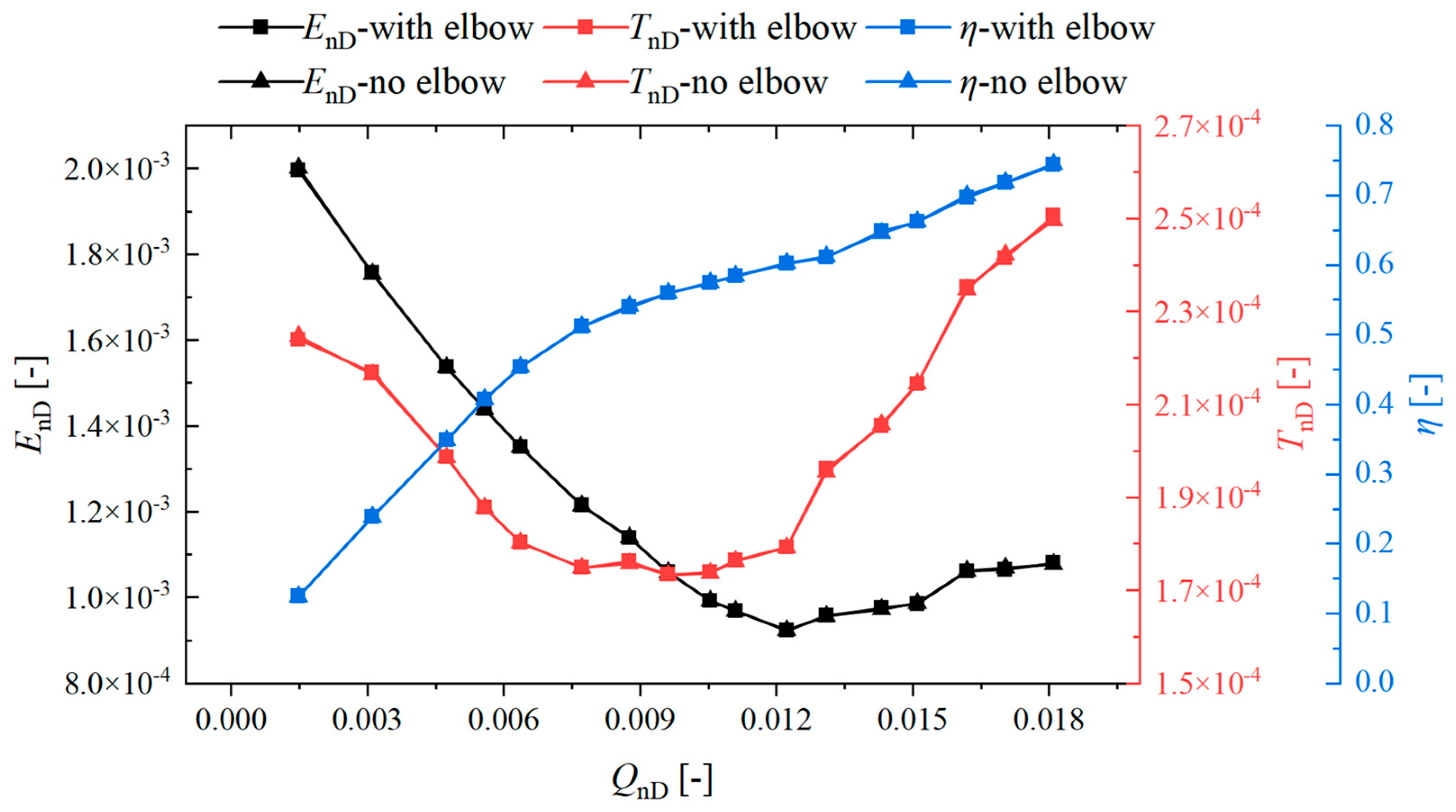
3.2. Energy Characteristic Curve Analysis

The hydraulic performance curve at a rotational speed of 750 r/min has been selected for analysis. During experiments, the second dip in the energy characteristic curve is approximately located at QnD = 0.012, and the peak is approximately at QnD = 0.015. At the dip, the difference between experimental and numerical simulation energy coefficients is around 10%, but they are essentially consistent in terms of flow coefficient. At the peak, the difference between experimental and numerical simulation energy coefficients is about 5%, with a flow coefficient deviation of approximately 20%. The experimental energy characteristic curve hump falls within the coverage range of the numerical simulation energy characteristic curve hump. The non-dimensionalized theoretical energy coefficient curves, including Et, EnD, and Eloss, are shown in Figure 12a. The yellow highlighted region in the figure represents the hump region. Figure 12b displays the slopes of these energy coefficient curves, with the hump position corresponding to the region where the curve slope changes from negative to positive and then back to negative. Figure 12c illustrates the changes in the curvature of the energy coefficient curves. From the graphs, it can be observed that before entering the hump region, the EnD energy coefficient curve maintains an upward curvature trend. In this trend, the descent of the EnD energy coefficient curve gradually decreases, and it starts to rise after reaching the valley. In the middle of the hump region, the curvature of the EnD energy coefficient curve changes from positive to negative, indicating that it starts to curve downward. Finally, the EnD energy coefficient curve gradually descends after reaching the peak.
The enlarged hump region in Figure 13 is shown. Although the theoretical energy coefficient (Et) curve consistently has a negative slope, indicating that the impeller’s work per unit fluid is always in a descending state, within the hump region, the slope of the theoretical energy coefficient (Et) curve is relatively small and, in some flow conditions, approaches zero. In contrast, the slope of the hydraulic loss energy coefficient (Eloss) curve is consistently positive. Ultimately, the sum of the slopes of the theoretical energy coefficient (Et) curve and the hydraulic loss energy coefficient (Eloss) curve is greater than zero, causing the energy characteristic curve to rise. From Figure 13b, it can be observed that the deviation of the theoretical energy coefficient (Et) curve plays a dominant positive role in the deviation of the energy coefficient (EnD) curve for QnD ≤ 0.013. However, at approximately QnD ≈ 0.014 and QnD ≈ 0.015, it has a negative effect, and at QnD ≥ 0.016, it has a positive effect of approximately equal magnitude to the deviation of the hydraulic loss energy coefficient (Eloss) curve. In the range 0.013 < QnD < 0.016, the contributions of the deviation of the theoretical energy coefficient (Et) curve and the hydraulic loss energy coefficient (Eloss) curve fluctuate significantly, suggesting significant changes in the internal flow state of the pump within this flow range.

3.3. Analysis of Entropy Generation in Pump

Figure 14 shows entropy production distribution contour maps at various axial heights in the impeller and guide vane passages, illustrating their distribution characteristics at valley and peak operating conditions. The figure reveals that at both valley and peak operating conditions, areas of high entropy production in the impeller passage are primarily near the blade tip. The guide vane passage exhibits high entropy production regions at various axial heights, with differing distribution patterns. Entropy production increases at the guide vanes’ inlet and decreases at the outlet with rising axial height. Additionally, at the valley condition, a high entropy production region is observed between the impeller and guide vane clearances near the hub. This is likely due to reduced axial spacing in that area, causing substantial flow disturbance from the interaction between rotating and stationary components. Furthermore, at the valley condition, overall entropy production in the impeller and guide vane passages across various axial heights exceeds that at the peak condition. The interaction between the impeller and guide vanes causes variations in entropy production distribution across different flow passages.

3.4. Analysis of Flow Characteristics in Pump

An analysis of internal flow characteristics, focusing on the relationship between flow structure, impeller performance, and internal flow losses at valley and peak conditions, is conducted using numerical simulation results.
(1) Blade load distribution
The aerodynamic forces on impeller blades correspond to their load distribution. Figure 15 shows the average load distribution on blades at various azimuthal positions for both valley and peak conditions. The figure indicates that at peak conditions, the pressure distribution on the impeller blades’ pressure side is higher and more uniform than at valley conditions. The pressure difference between the blade’s pressure and suction sides is more uniformly distributed at peak conditions and increases gradually with azimuthal angle. In contrast, at valley conditions, the pressure difference distribution between the pressure and suction sides is significantly varied.
The pressure difference is smaller near the blade’s leading edge and larger near the trailing edge, potentially causing flow separation. The area enclosed by the pressure distribution curve partly represents the impeller’s aerodynamic performance. The figure shows that for span ≥ 0.7, the impeller’s aerodynamic performance is better at peak than at valley flow conditions, with increasing performance difference from blade root to tip.
Figure 15 shows the average load distribution on all impeller blades. However, when the pump operates in the peak region, the flow inside the pump is quite complex, and there may be significant differences in the distribution patterns on different blades. To represent the pressure distribution on different blades of the impeller, the concept of pressure fluctuation coefficient Cp is introduced. It is used to characterize the magnitude of pressure variation on different blades relative to the average pressure on the blades. The expression for the pressure fluctuation coefficient Cp is as follows:
C p = P P ¯ 1 2 ρ U 2
In the formula, P is the pressure on different blades, the unit is Pa; P is the average pressure of all blades, the unit is Pa; ρ is the fluid density, the unit is kg/m3; and U is the circumferential velocity at the top of the inlet edge of the impeller blade, and the unit is m/s.
Figure 16 and Figure 17 show the pressure fluctuation coefficients on impeller blades at different circumferential positions. The left side of the figures represents the pressure side of the blades, while the right side represents the suction side. These figures illustrate the variations in pressure fluctuation coefficients during both valley and peak flow conditions.
Figure 16 illustrates that during valley flow conditions, there are notable variations in pressure fluctuations among different circumferential positions of the pressure side of the blades. In the front-middle section in the streamwise direction, the pressure side experiences significant pressure fluctuations. These fluctuations are relatively consistent across different circumferential positions. Towards the rear section in the streamwise direction, the pressure side still exhibits significant pressure fluctuations, but the discrepancies between circumferential positions become more evident. As circumferential height increases, the pressure fluctuations decrease in the rear section. It is worth noting that among the blades during the valley operating condition, Blade 5 and Blade 6 display larger pressure fluctuations compared to the other blades. On the other hand, during the valley operating condition, the suction side of the blade displays lower pressure fluctuations in the front section in the streamwise direction. However, as circumferential height increases, the pressure fluctuation on the suction side of the blade becomes more pronounced. In the middle to rear section in the streamwise direction, the suction side experiences relatively high pressure fluctuations, but these fluctuations decrease as circumferential height increases. Similar to the pressure side, when examining the pressure fluctuations on the suction side of the blades during the valley operating condition, Blade 1 and Blade 6 exhibit larger pressure fluctuations compared to the other blades. In conclusion, during valley flow conditions, significant variations in load distribution exist among different blades. Blade 1 shows higher pressure fluctuations on its suction side, while Blade 5 and Blade 6 have larger pressure fluctuations on both their pressure and suction sides. The flow patterns within the two channels formed by these three blades may exhibit increased complexity.
From Figure 17, it is evident that during peak flow conditions, the overall pressure fluctuations on the blades of the impeller are significantly smaller compared to valley flow conditions. There are only slight increases in pressure fluctuations in specific regions. These regions include the rear section in the streamwise direction at lower circumferential heights and the front section in the streamwise direction at higher circumferential heights. The areas with relatively higher pressure fluctuations are primarily observed on Blade 1’s suction side, Blade 2’s pressure side, and Blade 2’s suction side.
(2) Pressure distribution in the pump
To further analyze the pressure distribution and flow characteristics on different blade surfaces and within the flow passage at the conditions of valley and peak operating conditions, the pressure distribution contour maps at different spanwise heights within the impeller and guide vane regions are extracted, as shown in Figure 18. For convenience of description, the passage formed by Blade 1 and Blade 2 is referred to as Passage 1, and the others are denoted in the same manner. As can be seen from Figure 18a, at the valley operating condition, there is a region of low pressure in Passage 6, resulting in the pressure on certain areas of the suction side of Blade 1 and the pressure side of Blade 6 being lower than the average pressure on the blade. In Passage 5, the area’s pressure is slightly higher than in other passages, which ultimately leads to the pressure on certain areas of the pressure side of Blade 5 and the suction side of Blade 6 being lower than the average blade pressure. Additionally, scattered regions of high and low pressure within some passages were noted, indicating an uneven pressure distribution with significant variations, where complex flow structures such as backflow, secondary flow, and vortices may exist. Meanwhile, Figure 18b reveals that under the peak operating condition, only the pressure distribution near the leading edge area of Blade 2 at span = 0.9 shows a noticeable difference, while other areas exhibit higher consistency.
(3) Flow velocity distribution in the pump
In order to further investigate the state of flow within different channels under valley operating and peak operating conditions, the distribution of streamlines at different spanwise heights within the impeller and guide vane domains has been extracted, as illustrated in Figure 19. The distribution of streamlines on the axial cross-section is shown in Figure 20. Under valley operating conditions, there are significant recirculation vortices and flow separations within both the impeller and the guide vanes. With an increase in spanwise height, the occurrence of recirculation and separation progressively moves from the guide vanes to the impeller, where the formation of recirculation vortices obstructs the flow paths, ultimately leading to a reduction in the head of the waterjet propulsion pump. From Figure 19b, it is observable that at peak operating conditions, there is flow separation at higher spanwise locations of the impeller, and at lower spanwise positions of the guide vanes, smaller recirculation vortices are present. In regions other than these, the streamlines are smooth and evenly distributed, indicating a more regular flow pattern. The same observations can be inferred from Figure 20.

3.5. The Evolution Process of the Internal Rotating Stall of the Impeller in the Hump Region

To gain a deeper understanding of the rotating stall phenomenon within the impeller domain under valley operating conditions, the pressure distribution and velocity streamline diagrams at the spanwise height of span = 0.7 within the impeller domain were extracted for research and analysis.
Figure 21 shows the pressure distribution within the impeller at span = 0.7 under valley operating conditions. It is evident from the figure that the position of the stall vortex within the impeller corresponds closely to the low-pressure areas, with the circumferential propagation speed of the stall vortex being slower than the rotational speed of the blades. During valley operating conditions, two of the six flow channels in the impeller have large-scale stall vortex clusters. As the blades rotate, the position of the stall vortex clusters gradually moves from the suction side of one blade to the pressure side of the adjacent blade. Then, under the influence of the other blade, they are split into two smaller stall vortex clusters located near the inlet edge on both the pressure and suction sides of the same blade. With further rotation of the blade, the stall vortex on the pressure side weakens and eventually dissipates, while the vortex on the suction side strengthens and then repeats the aforementioned actions in a cyclical pattern.
When the stall vortex clusters transfer between channels, they are also accompanied by changes in the forces acting on the blades and the work done by them. When a stall vortex cluster is in the middle of a channel, although the channel is somewhat blocked, the difference in the forces acting on the blades on both sides of the channel is not significantly different from those in other channels. However, when the stall vortex cluster moves to the pressure side of a blade, the force state on that blade changes, the work done decreases, and the gap in the forces compared to other blades widens. During testing, it was found that when the pump enters the hump zone, the vibration and noise of the test pump intensify. The reason is that the change in the force state of individual blades disrupts the symmetrical distribution of forces on the impeller in space, causing vibration in the waterjet propulsion pump. As the stall vortex cluster continues to transfer, the blade with abnormal forces gradually recovers, and the next blade in the direction of the stall vortex propagation begins to change.

4. Experimental Study on Cavitation Structure in Hump Region

Operations in the hump region result in notably intensified vibrations and noise in pumps. Cavitation in impeller flow passages is observable through the impeller’s transparent casing. Cavitation notably impacts the thrust and propulsion efficiency of waterjet propulsors. Cavitation in waterjet pumps reduces propulsion efficiency and axial thrust, increasing vibration and noise, and can cause metallic erosion and damage to hydraulic component surfaces. This jeopardizes the operational stability of the waterjet propulsion system and the navigational safety of waterjet-propelled vessels. This chapter presents a study and analysis of the evolution of cavitation flow structures in pumps operating in the hump region, using high-speed photography technology.

4.1. The Critical Cavitation Stage of the Near Valley Condition

Figure 22 shows that during the critical cavitation phase near the surge valley, the flow channel predominantly exhibits vortex cavitation, cloud cavitation, and vertical cavitation vortices. These cavitation forms progress similarly to the first critical stage, with cloud cavitation starting near the impeller blade’s suction surface inlet edge. As the impeller rotates, cloud cavitation expands and eventually detaches, moving downstream with the rotating cavitation vortex clusters. Cavity size varies across flow channels; one channel is almost entirely blocked by cavities, while another is about one-third circumferentially blocked. At this point, the test pump exhibits an approximate 3% decrease in head under this flow condition compared to its initial state

4.2. The Critical Cavitation Stage of the Near Peak Condition

Figure 23 shows that during the critical cavitation phase near peak surge conditions, the flow channel mainly features vortex cavitation, blade tip leakage vortices, cloud cavitation, and vertical cavitation vortices. The cavitation flow structure evolution resembles that in the first critical phase, with cloud cavitation forming near the suction side’s inlet edge of the impeller blades. As the impeller rotates, this cavitation expands and detaches, moving downstream alongside the rotating cavitation vortex clusters. Compared to the first critical stage, cavity sizes within the flow channels have increased, though significant variance remains between different channels. In two adjacent channels, one might be nearly completely obstructed by cavities, while the other is about half-blocked circumferentially. At this stage, the test pump shows a 3% reduction in head under these flow conditions compared to the initial state.
The previous text reveals that the current model pump shows clear cavitation signs under both valley and peak operating conditions, even without using a vacuum pump to reduce inlet negative pressure. Cloud cavitation generation within a limited range is observable within the pump. As inlet negative pressure increases, cavitation bubbles begin to form, and cavity sizes progressively enlarge. At the valley operating condition, impeller channels mainly exhibit vortex cavitation, cloud cavitation, and vertical cavitation vortices. Conversely, at the peak operating condition, prevalent structures include vortex cavitation, blade tip leakage vortices, cloud cavitation, and vertical cavitation vortices. The main difference in cavitation flow between valley and peak conditions is the presence of blade tip leakage vortices at peak conditions, typically due to the pressure difference between the blade’s pressure and suction surfaces. At peak conditions, blade tip leakage vortices primarily occur at the blade tip’s front end, corresponding with areas of higher previously noted pressure difference. Additionally, at the same cavitation stage, cavity sizes inside the pump are slightly larger at peak conditions compared to valley conditions. The evolution process of cavitation structures is similar across different stages of development between valley and peak operating conditions.

5. Conclusions

This investigation employed experimental and numerical simulation methods to clarify the propulsion pump impeller’s performance, related internal flow losses, and flow dynamics. This study has provided insights into how variations in impeller performance and internal flow losses contribute to cavitation phenomena in the pump. Additionally, a comparative analysis was performed on the internal flow discrepancies between peak and valley operating conditions. The primary conclusions are as follows:
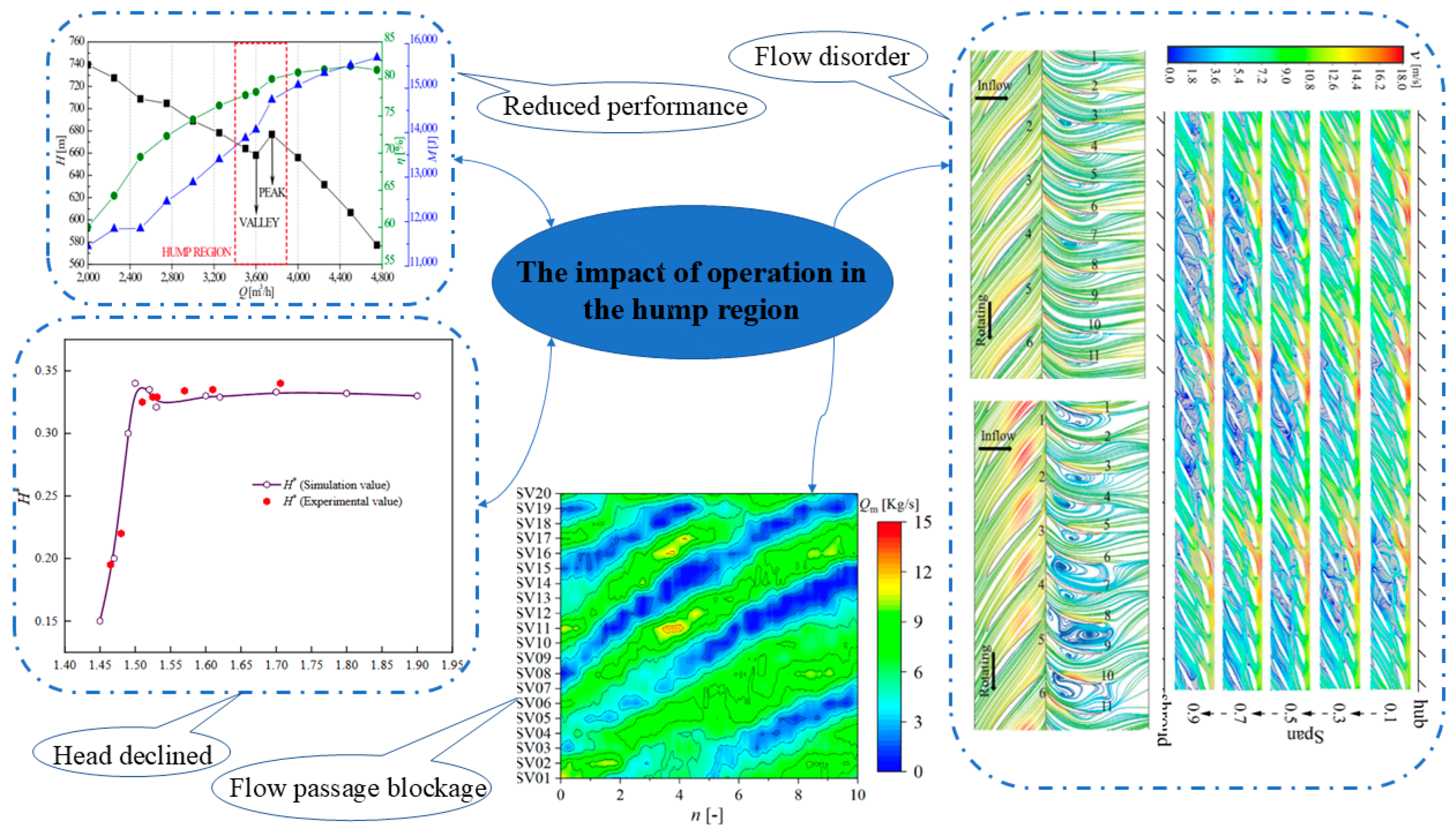
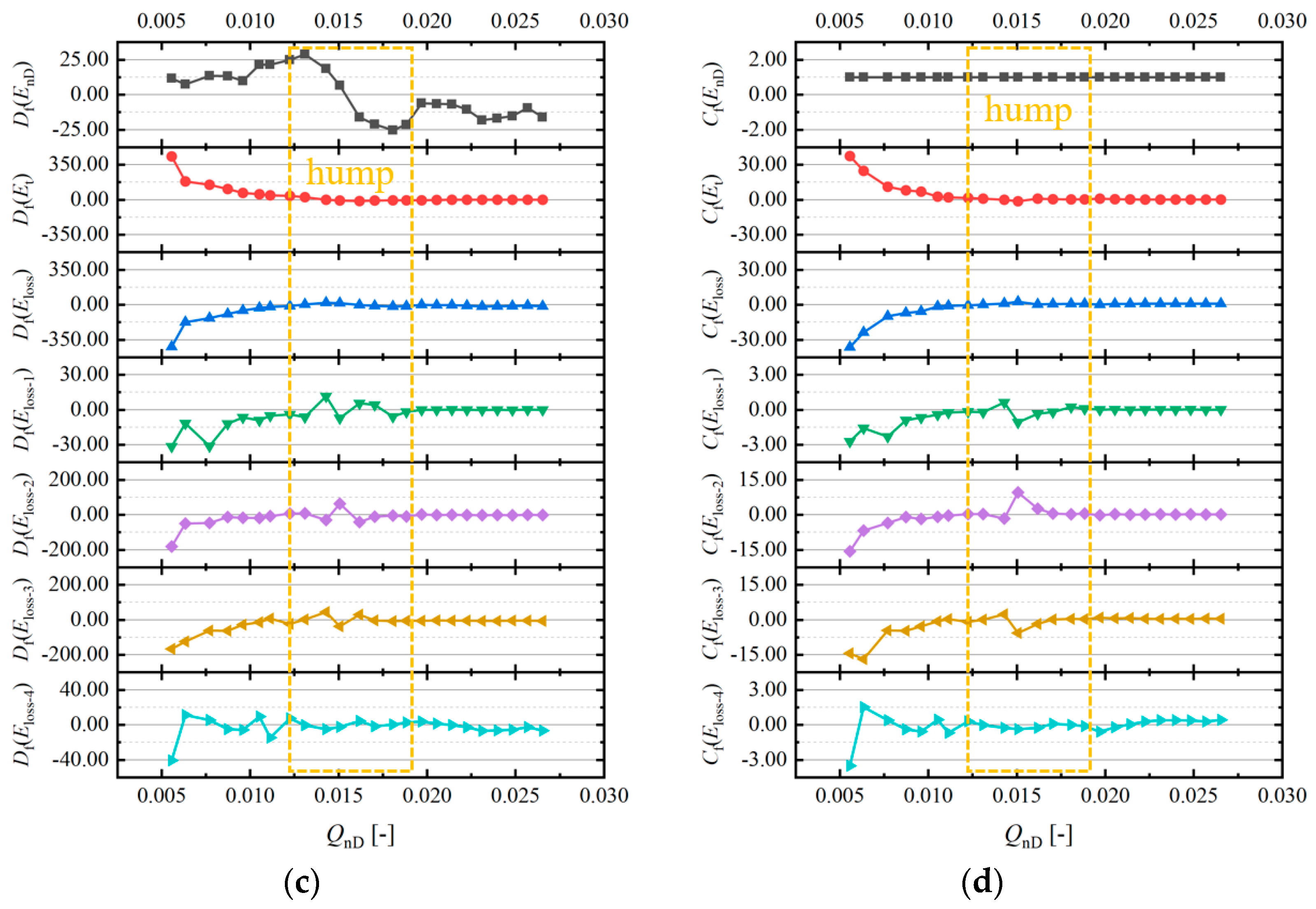
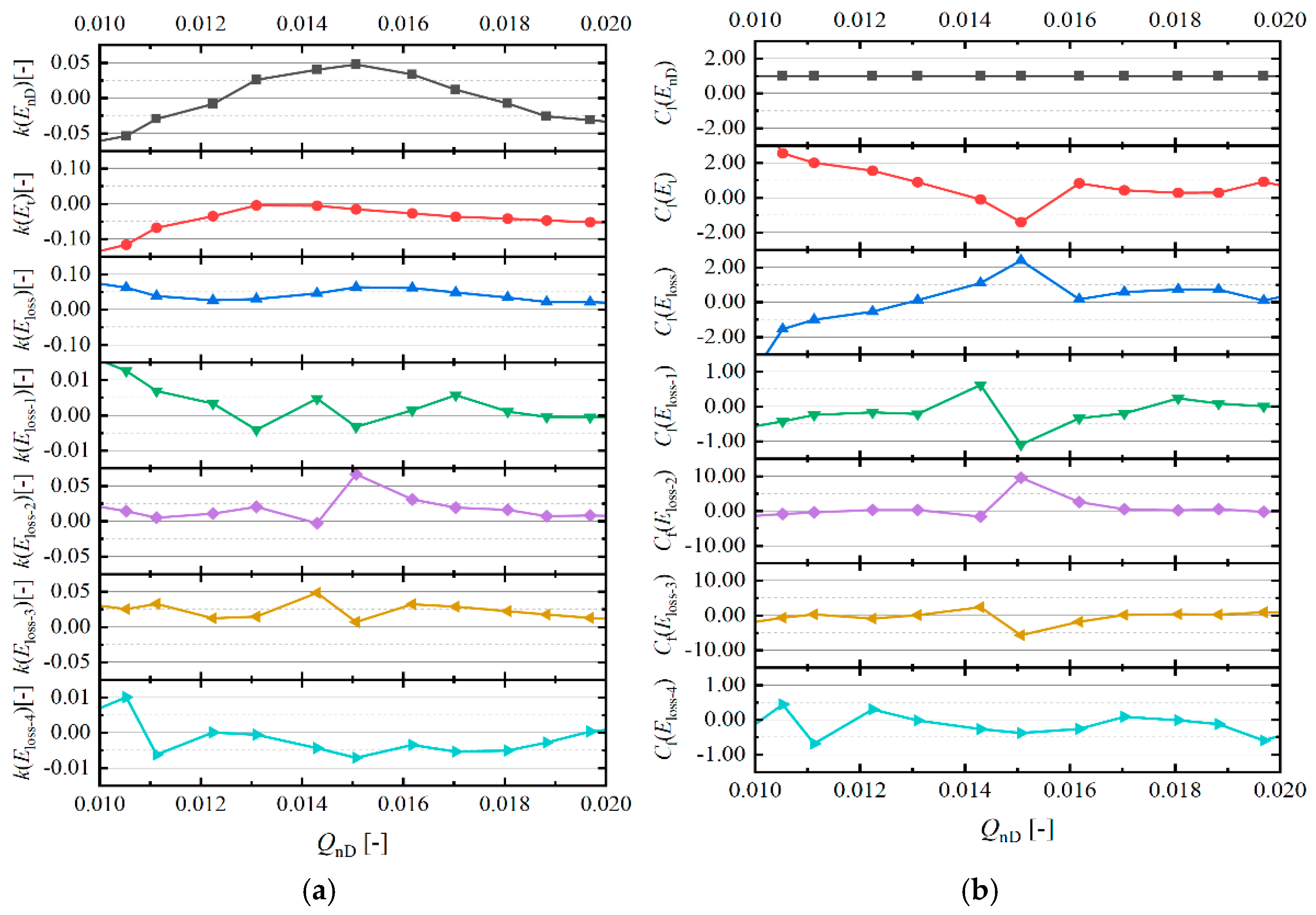
  • Utilizing a standard axial- or mixed-flow pump test bench and precise testing, this study compared impeller work on unit fluid and internal flow losses during hump formation through model pump energy characteristic curve analysis. The results indicate that at the onset of the hump, the decrease in work performed by the impeller on unit fluid diminishes, while internal fluid loss reduction increases. These factors collectively result in a counter-intuitive increase in the energy characteristic curve, contributing to hump formation.
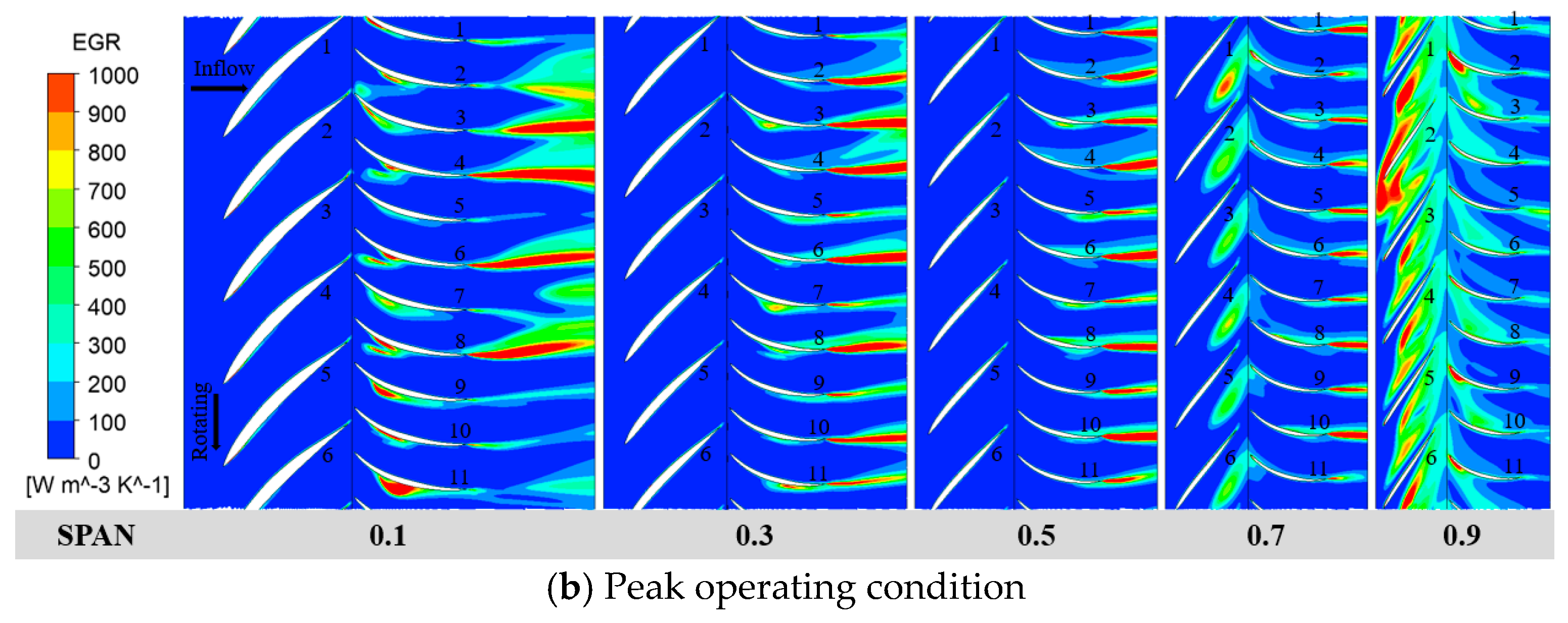
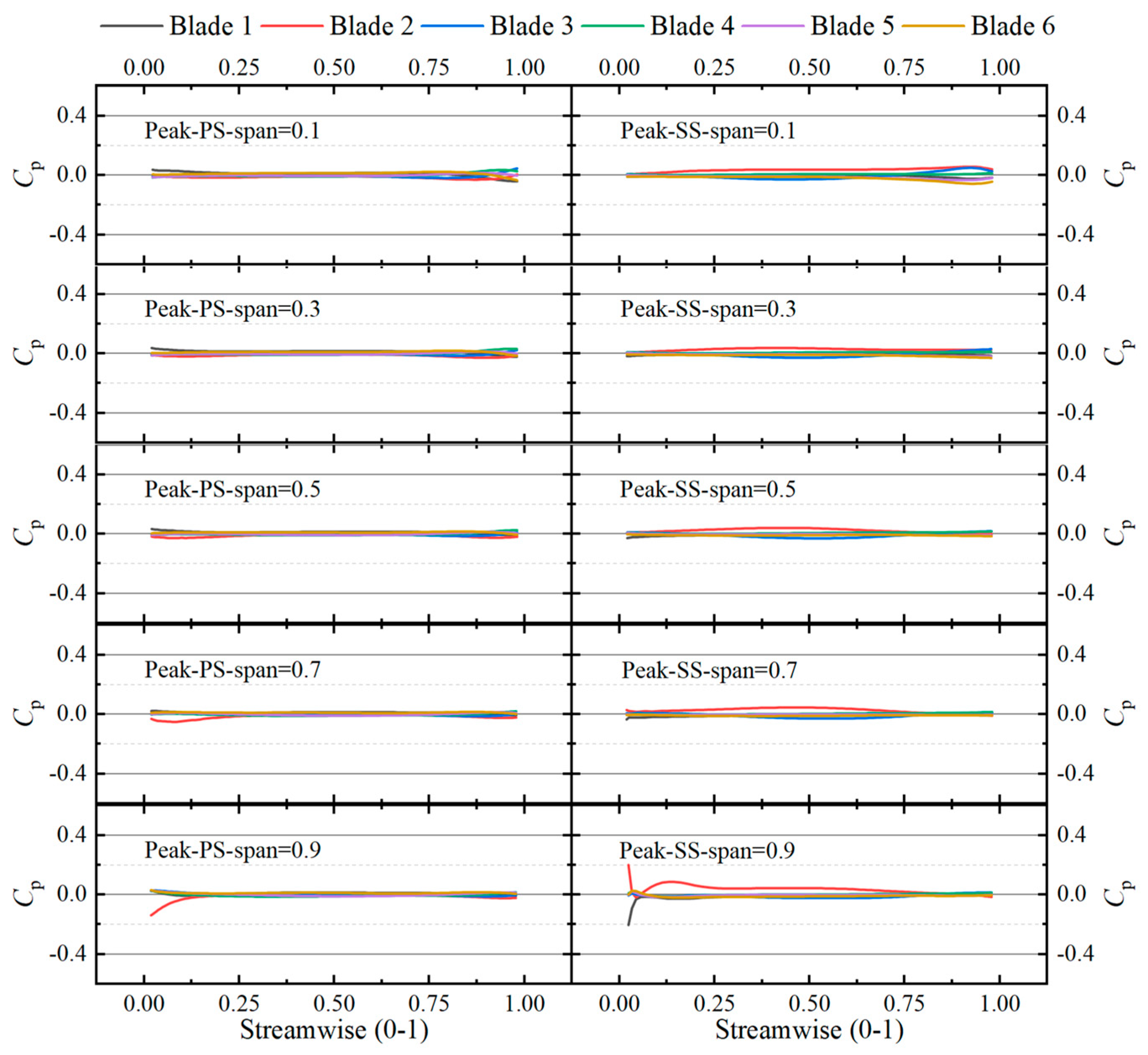
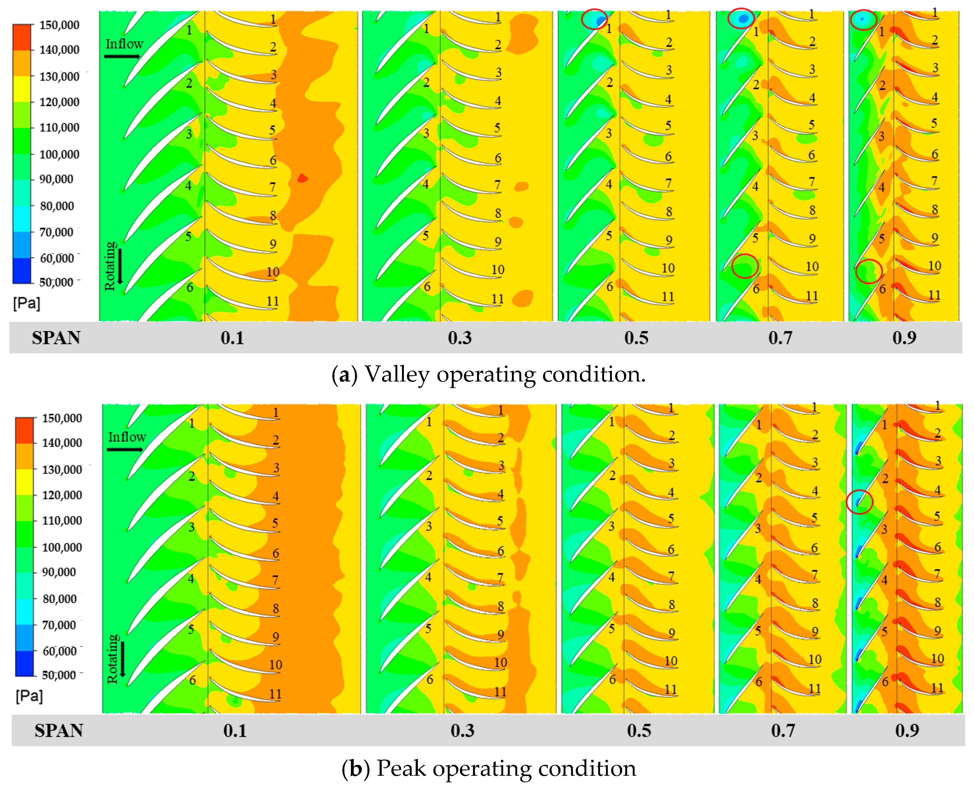
  • Compared to the valley condition, the impeller blades’ pressure surfaces at peak conditions exhibit higher and more uniform pressures, resulting in enhanced work performance. At the valley condition, flow losses primarily arise from the impeller, guide vanes, and draft tube, with guide vanes being the most significant contributors. At peak conditions, the loss distribution changes, showing reduced losses in the impeller and guide vanes, but increased losses in the draft tube. Turbulent dissipation is the main source of flow losses under both conditions. Particularly at the valley condition, substantial backflow vortices and flow separations near the impeller rim and guide vane hub increase flow losses, resulting in reduced head in the waterjet propulsion pump.
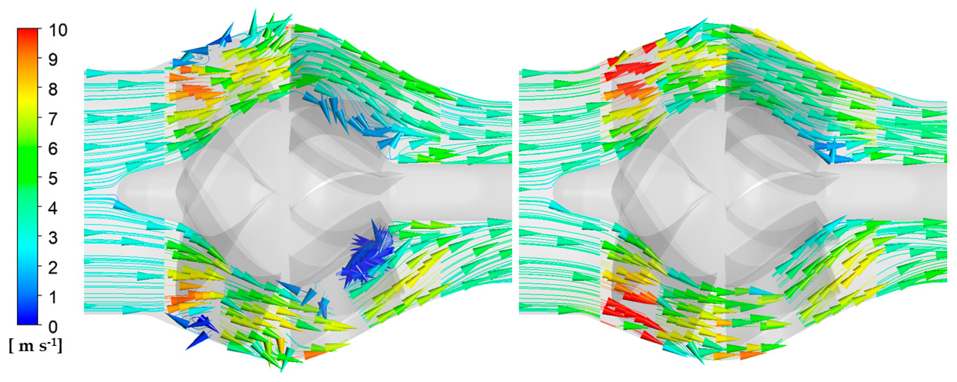
  • Under valley operating conditions, pressure and velocity distributions show significant variation across impeller channels, accompanied by prominent low-pressure areas that rotate with the impeller. These areas propagate circumferentially slower than the impeller’s rotation, leading to rotational stall, particularly in higher spanwise areas where vortices and flow separations occur. At peak conditions, pressure distribution is more uniform, and streamlines are smoother, with flow separation limited to high-span regions and minimal differences between channels. Overall, valley conditions reveal more intense vortex cores in the impeller and guide vanes, with large-scale vortex cores periodically growing and dissipating, alongside persistent vortices in the guide vane area.
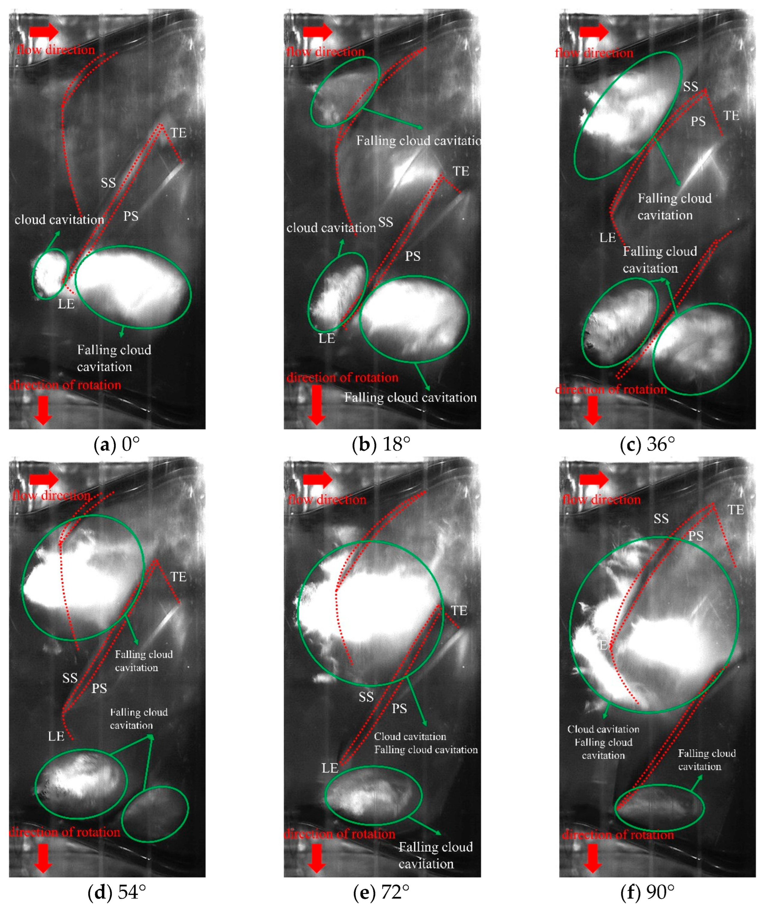
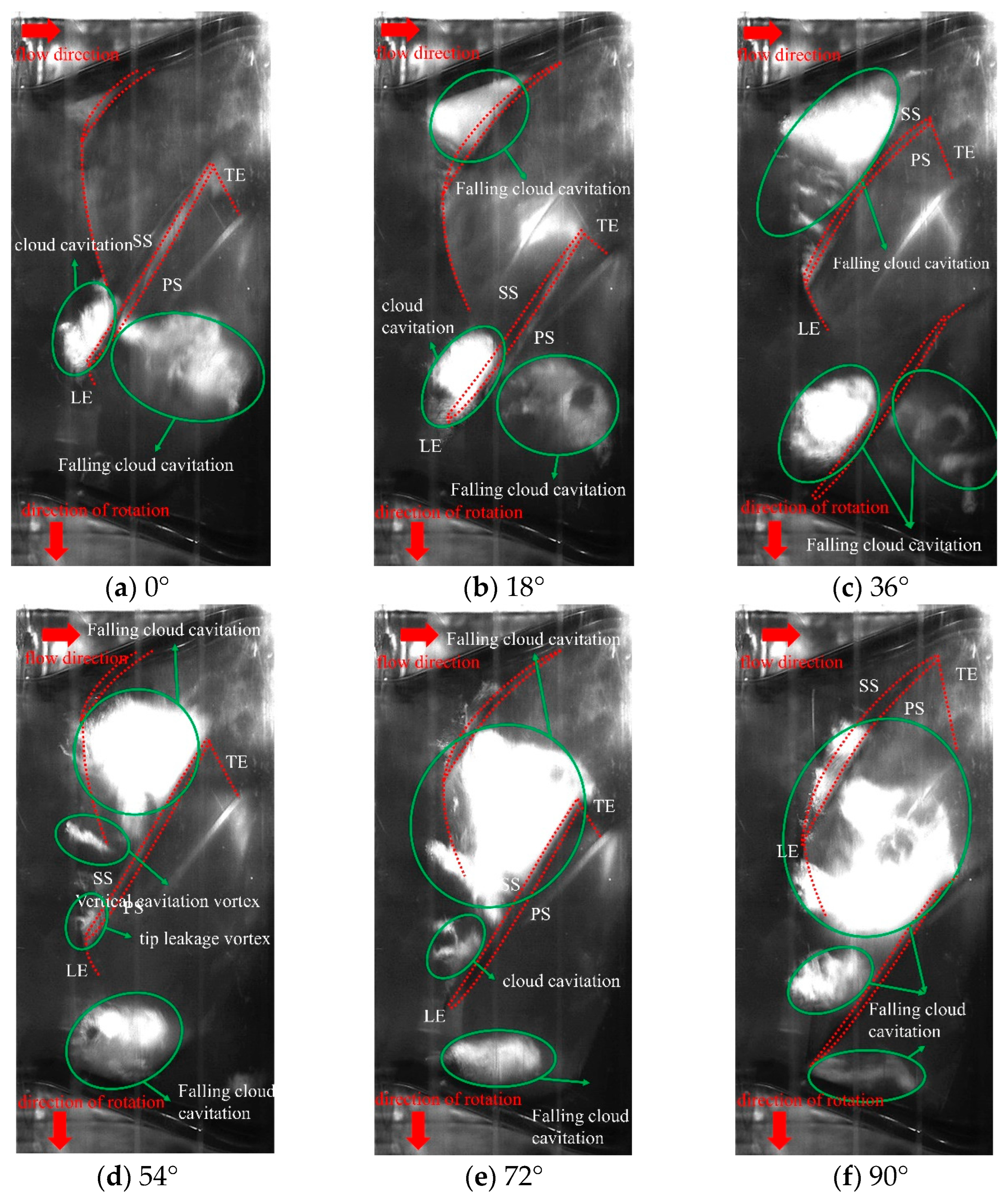
  • This study compares the evolution of cavitation flow structures during critical stages under near valley (QnD = 0.014) and peak (QnD = 0.016) operating conditions. The analysis highlights differences in cavitation flows within the pump, with forms like vortex cavitation, cloud cavitation, and vertical cavitation vortices noted at valley operating conditions. At peak conditions, cavitation forms are similar to those at valley conditions, but larger blade tip leakage vortices occur, attributed to increased pressure differences between the impeller blades’ pressure and suction sides.

Author Contributions

Conceptualization, Y.L.; Resources, M.L. and H.Y.; Writing—original draft, J.Z.; Writing—review & editing, C.T. All authors have read and agreed to the published version of the manuscript.

Funding

This work is funded by the China Postdoctoral Science Foundation Funded Project (Grant No. 2023M733355), Research Project of State Key Laboratory of Mechanical System and Vibration (Grant No. MSV202203), Natural Science Foundation of China (Grant No. 51906085, U20A20292), Jiangsu University Youth Talent Development Program (2020), and the Chunhui Program Cooperative Scientific Research Project of the Ministry of Education.

Institutional Review Board Statement

Not applicable.

Informed Consent Statement

Not applicable.

Data Availability Statement

Data will be made available upon request.

Conflicts of Interest

The authors declare that they have no known competing financial interests or personal relationships that could have appeared to influence the work reported in this paper.

References

  1. Li, W.; Zhou, L.; Shi, W.-D.; Ji, L.; Yang, Y.; Zhao, X. PIV experiment of the unsteady flow field in mixed-flow pump under part loading condition. Exp. Therm. Fluid Sci. 2017, 83, 191–199. [Google Scholar] [CrossRef]
  2. van Esch, B.P.M.; Kruyt, N.P. Hydraulic performance of a mixed-flow pump: Unsteady inviscid computations and loss models. J. Fluids Eng.-Trans. ASME 2001, 123, 256–264. [Google Scholar] [CrossRef]
  3. Heo, M.-W.; Kim, K.-Y.; Kim, J.-H.; Choi, Y.S. High-efficiency design of a mixed-flow pump using a surrogate model. J. Mech. Sci. Technol. 2016, 30, 541–547. [Google Scholar] [CrossRef]
  4. Suh, J.-W.; Yang, H.-M.; Kim, Y.-I.; Lee, K.-Y.; Kim, J.-H.; Joo, W.-G.; Choi, Y.-S. Multi-objective optimization of a high efficiency and suction performance for mixed-flow pump impeller. Eng. Appl. Comput. Fluid Mech. 2019, 13, 744–762. [Google Scholar] [CrossRef]
  5. Yun, L. Study on the Hydraulic Optimization Design Method and Cavitation of Waterjet Pump. Ph.D. Dissertation, Shanghai Jiao Tong University, Shanghai, China, 2018. [Google Scholar]
  6. Yun, L.; Chao, F.; Luyi, W.; Dezhong, W.; Youlin, C.; Rongsheng, Z. Experiment on cavitation flow in critical cavitation condition of water-jet propulsion pump. J. Beijing Univ. Aeronaut. Astronaut. 2019, 45, 1512–1518. [Google Scholar]
  7. Long, Y.; An, C.; Zhu, R.; Chen, J. Research on hydrodynamics of high velocity regions in a water-jet pump based on experimental and numerical calculations at different cavitation conditions. Phys. Fluids 2021, 33, 045124. [Google Scholar] [CrossRef]
  8. Niazi, S.; Stein, A.; Sankar, L. Numerical studies of stall and surge alleviation in a high-speed transonic fan rotor. In Proceedings of the 38th Aerospace Sciences Meeting and Exhibit, Reno, NV, USA, 10–13 January 2000; p. 225. [Google Scholar]
  9. Shahriyari, M.J.; Khaleghi, H.; Heinrich, M. A Model for Stall and Surge in Low-Speed Contra-Rotating Fans. J. Eng. Gas Turbines Power-Trans. Asme 2019, 141, 081009. [Google Scholar] [CrossRef]
  10. Ye, W.; Ikuta, A.; Chen, Y.; Miyagawa, K.; Luo, X. Numerical simulation on role of the rotating stall on the hump characteristic in a mixed fl ow pump using modi fi ed partially averaged Navier-Stokes model. Renew. Energy 2020, 166, 91–107. [Google Scholar] [CrossRef]
  11. Yang, J.; Yuan, S.; Pavesi, G.; Chun, L.; Zhou, Y. Study of hump instability phenomena in pump turbine at large partial flow conditions on pump mode. Jixie Goneheng Xuebao 2016, 52, 170–178. [Google Scholar] [CrossRef]
  12. Pavesi, G.; Yang, J.; Cavazzini, G.; Ardizzon, G. Experimental analysis of instability phenomena in a high-head reversible pump-turbine at large partial flow condition. In Proceedings of the 11th European Conference on Turbomachinery Fluid Dynamics and Thermodynamics, Madrid, Spain, 23–26 March 2015. [Google Scholar]
  13. Pavesi, G.; Cavazzini, G.; Ardizzon, G. Numerical Analysis of the Transient Behaviour of a Variable Speed Pump-Turbine during a Pumping Power Reduction Scenario. Energies 2016, 9, 534. [Google Scholar] [CrossRef]
  14. Jese, U.; Fortes-Patella, R.; Dular, M. Numerical study of pump-turbine instabilities under pumping mode off-design conditions. In Proceedings of the ASME-JSME-KSME Joint Fluids Engineering Conference (AJK-FED), Seoul, Republic of Korea, 26–31 July 2015. [Google Scholar]
  15. Braun, O.; Kueny, J.L.; Avellan, F. Numerical analysis of flow phenomena related to the unstable energy-discharge characteristic of a pump-turbine in pump mode. In Proceedings of the ASME Fluids Engineering Division Summer Meeting, Houston, TX, USA, 19–23 June 2005; pp. 1075–1080. [Google Scholar]
  16. Li, D.; Zhu, Y.; Lin, S.; Gong, R.; Wang, H.; Luo, X. Cavitation effects on pressure fluctuation in pump-turbine hump region. J. Energy Storage 2022, 47, 103936. [Google Scholar] [CrossRef]
  17. Long, Y.; Tian, C.; Li, Y.; Zhong, J. Internal Flow Mechanism of the Water jet Pump at Crest and Trough Conditions in the Hump Region. Ship Boat 2023, 34, 56. [Google Scholar]
  18. Yang, J.; Feng, X.; Liu, X.; Peng, T.; Chen, Z.; Wang, Z. The suppression of hump instability inside a pump turbine in pump mode using water injection control. Processes 2023, 11, 1647. [Google Scholar] [CrossRef]
  19. Zhu, R.; Shi, W.; Gan, G.; Li, H.; Yang, D.; Duan, Y.; Fu, Q. Transient Hydrodynamic Characteristics of a High-Speed Axial Flow Water-Jet Pump during Variable Speed Process. J. Mar. Sci. Eng. 2023, 11, 1965. [Google Scholar] [CrossRef]
  20. Han, H.; Long, Y.; Zhong, J. Research on the internal flow difference between peak and valley conditions of water jet propulsion pump during working at hump region. J. Mar. Sci. Eng. 2024, 12, 258. [Google Scholar] [CrossRef]
  21. Long, Y.; Zheng, Y.; Han, H.; Zhong, J.; Zhu, R. Research on hydraulic optimization design method of water-jet propulsion pump considering hump index. J. Braz. Soc. Mech. Sci. Eng. 2024, 46, 377. [Google Scholar] [CrossRef]
  22. Long, Y.; Zhou, Z.; Zhong, J.; Han, H. Experimental Study on Evolution of Cavitation Flow Structure in Hump Region of Waterjet Pump. J. Appl. Fluid Mech. 2024, 17, 2734–2744. [Google Scholar]
  23. Kock, F.; Herwig, H.J.I.J.O.H. Local entropy production in turbulent shear flows: A high-Reynolds number model with wall functions. Int. J. Heat Mass Transf. 2004, 47, 2205–2215. [Google Scholar] [CrossRef]
Figure 1. Schematic diagram of waterjet propulsion pump structure.
Jmse 13 00442 g001
Figure 2. Diagram of hump phenomenon.
Jmse 13 00442 g002
Figure 3. The effect of the hump region on the hydrodynamic performance of the pump [16,17,18,19].
Jmse 13 00442 g003
Figure 4. Components of the test model pump.
Jmse 13 00442 g004
Figure 5. Schematic of axial- or mixed-flow pump test loop [20].
Jmse 13 00442 g005
Figure 6. Installation diagram of the test pump section.
Jmse 13 00442 g006
Figure 7. Test site for the model pump.
Jmse 13 00442 g007
Figure 8. Numerical simulation results of two computational fluid domain schemes [21].
Jmse 13 00442 g008
Figure 9. Computational grid.
Jmse 13 00442 g009
Figure 10. Local grids of hydraulic components.
Jmse 13 00442 g010
Figure 11. Composition of grid numbers for different schemes and their CFD results [22].
Jmse 13 00442 g011
Figure 12. Analysis of energy characteristic curves. (a) Energy coefficient curve. (b) Slope change of energy coefficient curve. (c) Deflection change. (d) Variation of deflection contribution factor.
Jmse 13 00442 g012aJmse 13 00442 g012b
Figure 13. Analysis of energy characteristic curves in the hump region. (a) The slope change of the energy coefficient curve in the hump region. (b) The variation of the deflection contribution factor in the hump region.
Jmse 13 00442 g013
Figure 14. Distribution of entropy generation in pump.
Jmse 13 00442 g014aJmse 13 00442 g014b
Figure 15. The average load distribution in different spans.
Jmse 13 00442 g015
Figure 16. Pressure fluctuations of different blades of the impeller under valley operating condition.
Jmse 13 00442 g016
Figure 17. Pressure fluctuations of different blades of the impeller under peak operating condition.
Jmse 13 00442 g017
Figure 18. The pressure distribution under valley operating and peak operating conditions.
Jmse 13 00442 g018
Figure 19. Streamline distribution of inside the pump under valley and peak operating conditions.
Jmse 13 00442 g019
Figure 20. The axial cross-section streamline distribution under valley operating and peak operating conditions.
Jmse 13 00442 g020
Figure 21. The pressure distribution within the impeller at span = 0.7 under valley operating conditions.
Jmse 13 00442 g021
Figure 22. The cavitation flow structure and its evolution law under the critical cavitation stage in the near valley operating condition.
Jmse 13 00442 g022
Figure 23. The cavitation flow structure and its evolution law under the critical cavitation stage in the near peak operating condition.
Jmse 13 00442 g023
Table 1. Parameters of the test pump.
ParameterNumerical Value
Impeller inlet diameter250 mm
Number of impeller blades6
Number of guide vanes11
Exit diameter183 mm
Maximum design speed1500 r/min
Design point flow at the highest design speed1660 m3/h
Design point head at the highest design speed≥17 m
Tip clearance1 mm
Table 2. Wall Y+ values of each component.
UnitWall ShearWall MinimumWall MaximumWall AverageComponent Average
Inlet pipePipe wall1.08315.8824.1104.151
Propeller cap1.16817.7276.549
ImpellerHub0.0384.7392.0043.504
Blade0.05115.6734.212
Wheel rim0.13110.2023.198
DiffuserHub0.0497.1502.0753.714
Blade0.04110.3304.035
Wheel rim0.13110.2023.937
Outlet pipeAxis5.49512.7378.0007.518
Pipe wall5.3239.8577.368
Table 3. Setting of boundary conditions for steady calculation.
Settings ItemParameters
Inlet boundary conditionPressure
Outlet boundary conditionMass flow rate
Wall boundary conditionNo-slip wall
Turbulence modelSST k-ω
Interface between static and dynamicFrozen rotor
Convergent residuals (math.)10−4
Disclaimer/Publisher’s Note: The statements, opinions and data contained in all publications are solely those of the individual author(s) and contributor(s) and not of MDPI and/or the editor(s). MDPI and/or the editor(s) disclaim responsibility for any injury to people or property resulting from any ideas, methods, instructions or products referred to in the content.

