Article

Three-Dimensional In Situ Stress Distribution in a Fault Fracture Reservoir, Linnan Sag, Bohai Bay Basin

1
School of Geoscience, China University of Petroleum (East China), Qingdao 266580, China
2
National Key Laboratory of Deep Oil and Gas, China University of Petroleum (East China), Qingdao 266580, China
*
Authors to whom correspondence should be addressed.
J. Mar. Sci. Eng. 2025, 13(3), 436; https://doi.org/10.3390/jmse13030436
Submission received: 14 January 2025 / Revised: 10 February 2025 / Accepted: 21 February 2025 / Published: 25 February 2025
(This article belongs to the Section Geological Oceanography)

Abstract

:
The fault fracture body, consisting of faults, fracture zones, cracks, and the matrix, plays a crucial role in controlling oil and gas accumulation. Understanding its spatial distribution and analyzing the in situ stress field are essential for optimizing well design and fracturing operations. This study integrates geological, logging, and seismic data, and employs advanced techniques such as ant tracking to establish a skeletal model of the fault fracture body. Reverse modeling and optimization reconstruction are used to construct a three-dimensional geomechanical model of the fracture system. Machine learning techniques, specifically a back propagation (BP) neural network, are utilized to invert the boundary conditions of the study area. Finite element numerical simulation software is then applied to model the three-dimensional in situ stress field under coupled flow–solid interaction. The reservoirs in the study area are characterized by a dense structure, low porosity, and low permeability. The results indicate that the maximum horizontal principal stress in the fault fracture reservoir ranges from 68.0 to 72.8 MPa, while the minimum horizontal principal stress ranges from 58.2 to 63.1 MPa. The stress at fractures is lower than that in the surrounding matrix, and stress concentrations occur at both ends of the faults. The in situ stress field exhibits distinct subarea characteristics, with significant stress reductions across fault fractures and directional deflections at faults. These findings provide valuable insights for improving reservoir development efficiency and optimizing well operations in similar geological settings.

1. Introduction

Fault-fractured reservoirs have a significant influence on fluid flow by enhancing the effective permeability of the porous media, which refers to the ability of the rock to allow fluids to flow through it, considering the presence of fractures and other flow pathways [1,2]. The fracture exploitation system and its integration with faults, known as the fault fracture system, plays a more critical role in practical exploration and exploitation than individual faults or fractures [3]. Meanwhile, in situ stress serves as a vital parameter for well placement and sweet spot evaluation, significantly impacting the transportation and extraction processes. Therefore, understanding the distribution characteristics of the in situ stress field in fracture-seam reservoirs is an important way to improve the economic efficiency of oilfields.
Ever since the large-scale exploitation of fractured reservoirs began in the 1970s, the results of exploiting most fractured reservoirs have not been satisfactory. Even when frac reservoirs are exploited successfully and economically, recovery rates are typically maintained at 13–15%, indicating potential for improvement [4]. This situation is partly due to a limited understanding of fracture identification, distribution laws, and fluid flow dynamics within fractures [5]. Consequently, the accurate identification of complex fault and fracture information is pivotal for exploration and exploitation. Fracture identification methods can be categorized into direct methods, such as core observations, thin section and FE-SEM analysis, and FMI logging, and indirect methods, which involve processing and analyzing conventional logging curves [6]. In many naturally fractured reservoirs, fractures are often induced or reactivated by faulting, necessitating a combined modeling of faults and fractures. A reliable reservoir model of fault zones requires a comprehensive analysis of seismic and logging data to understand the tectonic characteristics of faults and fractures. Tuong et al. and Adrià et al. developed characteristic parameters from conventional logging data to highlight fracture responses and established a conventional logging fracture model [7,8]. Lyu et al. enhanced fracture identification accuracy within fault seams by introducing the integrated index method and fractal method [9]. Zhang et al. created a mathematical model for fracture permeability variation with pressure based on material balances in fractured reservoir production [10]. Laubach et al. proposed a method to record natural fracture trends in sandstone layers, applicable even in boreholes without visible fractures [11]. Velázquez et al. and Jarosinski et al. utilized the ANSYS finite element software to calculate stress fields and predict fracture distributions [12,13]. Sollberger et al. and Brossier et al. improved seismic interpretation by reducing inversion degrees of freedom, enhancing interpretation capabilities, and establishing three-dimensional lithofacies models using sequence index simulation algorithms [14,15]. Numerical simulation methods are essential for accurately describing the in situ stress field within reservoirs, providing stress values at different layers and facilitating the investigation of stress distribution characteristics. Miao et al. conducted numerical simulations to identify factors influencing in situ stress during flow–solid coupling, finding that stress distribution is closely related to the number and orientation of faults in the study area [16]. Moinfar et al. proposed a coupled flow and geomechanical model using an embedded discrete fracture Model (EDFM) for reservoirs with complex fracture networks [17]. Liu et al. obtained the in situ stress distribution law of vertical multi-interbedded layers with different lithologies by interpreting in situ stress logging results of a single well, combined with the geological, structural, and sedimentary characteristics of the block [18]. Papanastasiou et al. investigated the in situ stress field of the Levantine Basin of the Eastern Mediterranean using finite element analysis combined with the poroelasto-plasticity theory, finding that tectonic activity significantly increases horizontal stresses, and fault surface sliding conditions substantially impact the stress field [19].
Previous studies have significantly advanced the understanding of fracture identification and in situ stress field analysis in fractured reservoirs. At present, the understanding of the in situ stress field distribution in fault-fractured reservoirs is relatively limited. Existing numerical simulation models often resort to oversimplification, neglecting crucial geological features such as faults and fractures. To address these limitations, this study aims to construct a geomechanical model of a fractured reservoir, reflecting authentic stratigraphic conditions.
The lower sub-member of the 3rd member of Shahejie Formation fractured reservoir in the Jiangjiadian region of the Linnan Sag serves as a case study. This study investigates the three-dimensional in situ stress distribution in the shale reservoir of the Linnan Sag in the Bohai Bay Basin by integrating machine learning and numerical simulation methods. The BP neural network, a type of multilayer feedforward neural network, possesses robust nonlinear mapping capabilities, making it suitable for addressing the complex nonlinear relationships between stress and load in geological environments. By inputting the measured maximum and minimum horizontal principal stress values at well points into the trained BP neural network model, the boundary load values of the fracture model in the study area can be predicted.
The three-dimensional in situ stress field is simulated using finite element numerical simulation software, considering the coupling effects of fluid and solid mechanics. The control equations are established to simulate the stress field distribution within the reservoir. The analysis of the simulation results reveals the distribution characteristics and directional variations of the maximum and minimum horizontal principal stresses in the fracture reservoir under both uncoupled and coupled flow–solid conditions. The utilization of machine learning techniques enables the handling of complex nonlinear relationships, providing a more accurate representation of the stress–load interactions in actual formations compared to traditional linear models or empirical formulas. Traditional in situ stress simulation methods often neglect the interactions between fluid and rock skeleton, whereas the coupled flow–solid control equations offer a more realistic depiction of the stress distribution in reservoirs, especially when fluid flow significantly affects the mechanical properties of the rock.

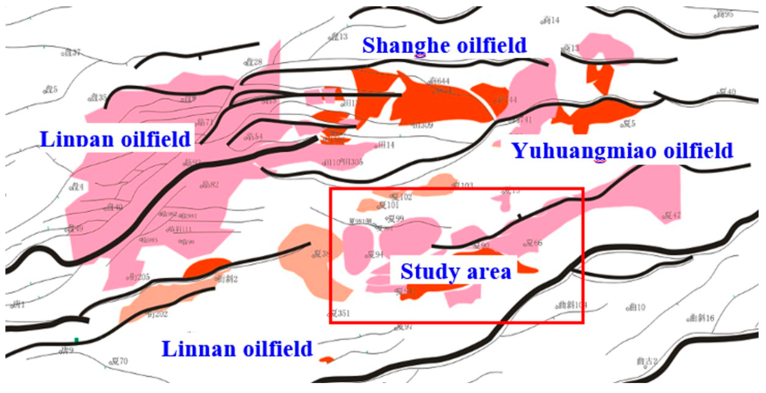
2. Geological Profile of the Study Area

2.1. Structural Characteristics of the Study Area

The study area is located in the Linnan Sag, which is part of the Huimin Depression in the Bohai Bay Basin, as shown in Figure 1. The tectonic evolution of the study area is complex and is primarily controlled by north–south trending faults, especially the northeast-striking Xiakou Fracture Zone. The main oil-bearing interval is the third member of the Shahejie Formation (Es3), which is characterized by a complex sedimentary environment, including shallow marine, deep marine, and submarine slope settings. The sedimentary characteristics of the Es3 member are marked by overall deep subsidence and water body expansion during the deposition period. The sediments are predominantly fine-grained, forming organic-rich shales with good potential for hydrocarbon generation. The sedimentary cycles of the Es3 member are distinct, with early deposition occurring in deepwater slope settings, a shift to shallow marine environments in the middle stage, and a return to deep marine conditions in the late stage. These complex tectonic and sedimentary characteristics have significant impacts on hydrocarbon generation, storage, and migration. The fault systems not only control the distribution of sedimentary environments but also provide pathways for hydrocarbon migration. The complex sedimentary cycles and lithologic variations result in heterogeneous reservoirs, posing challenges for hydrocarbon exploration and exploitation. The area extends from the Xiakou Fracture Zone in the south to the Central Backslope Belt in the north. The plunging anticlines of Jiangjadian and Waya are aligned along the descending plate of the Xiakou Fracture Zone, a tectonic boundary where one plate is subducting beneath another, extending from west to east. The tectonic evolution of the Jiangjiadian area is both regional and temporal, and it is intricately linked to the complex fracture system.

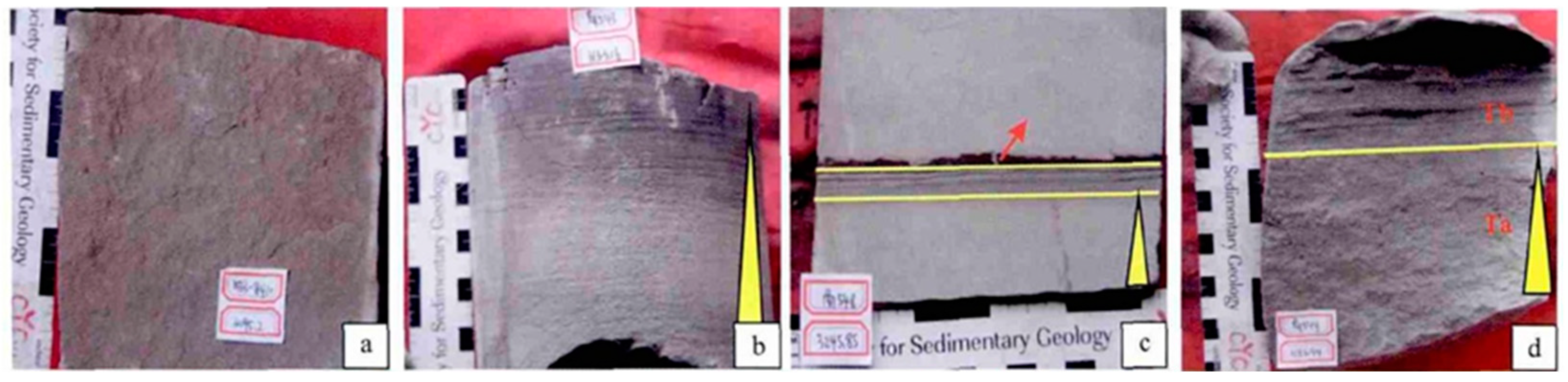
2.2. Sedimentary Characteristics of the Study Area

The depositional characteristics are closely related to the complex fault system. The 3rd member of the Shahejie Formation of the Linnan Sag in the Bohai Bay Basin is the primary oil-bearing interval, with overall deep subsidence and water body expansion during the deposition period. The sedimentary environment is complex, encompassing shallow marine, deep marine, and submarine slope settings. In deepwater environments, finer-grained sediments form organic-rich shale deposits (Figure 2). Shales in deepwater environments typically exhibit higher organic matter content and are primarily wetland–deepwater mixed facies, which have good oil and gas generation potential. The shale reservoirs of the lower sub-member of the 3rd member of the Shahejie Formation in the study area are dense, with low porosity and permeability. However, fractures are well developed, mainly consisting of high-angle and vertical fractures, forming a complex fracture network system, which enhances the gas and oil storage capacity.

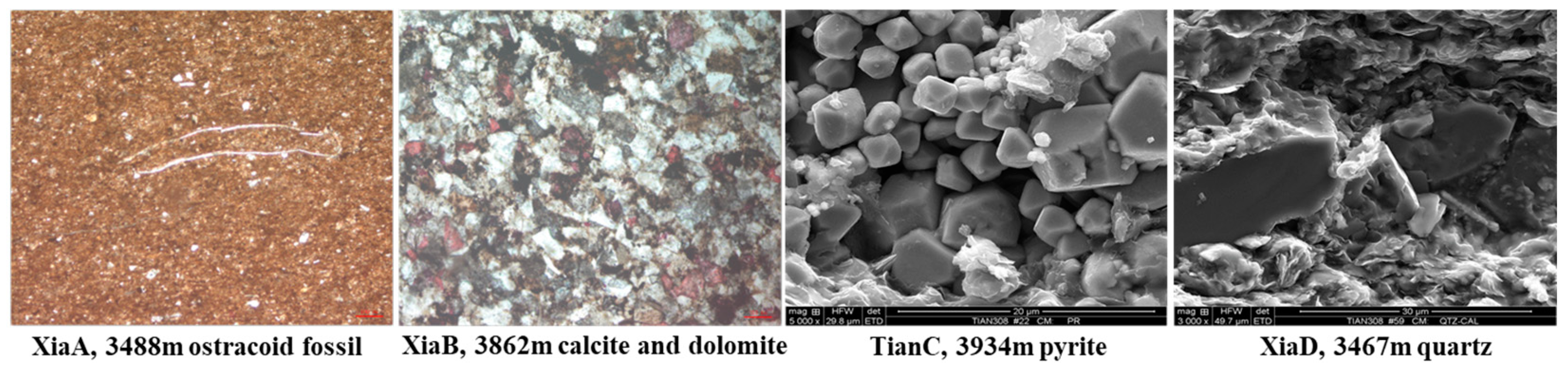
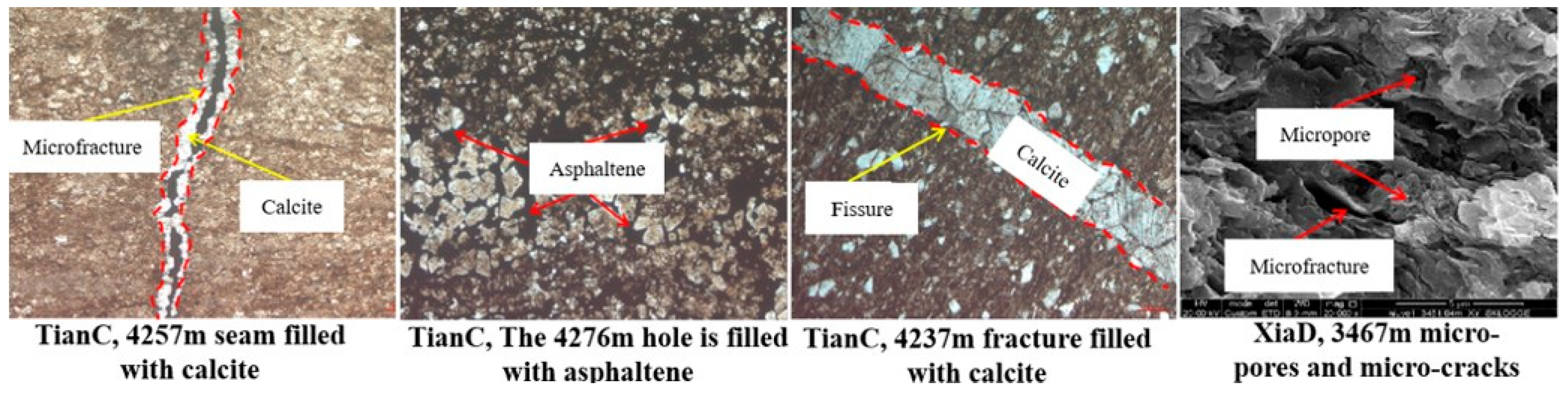
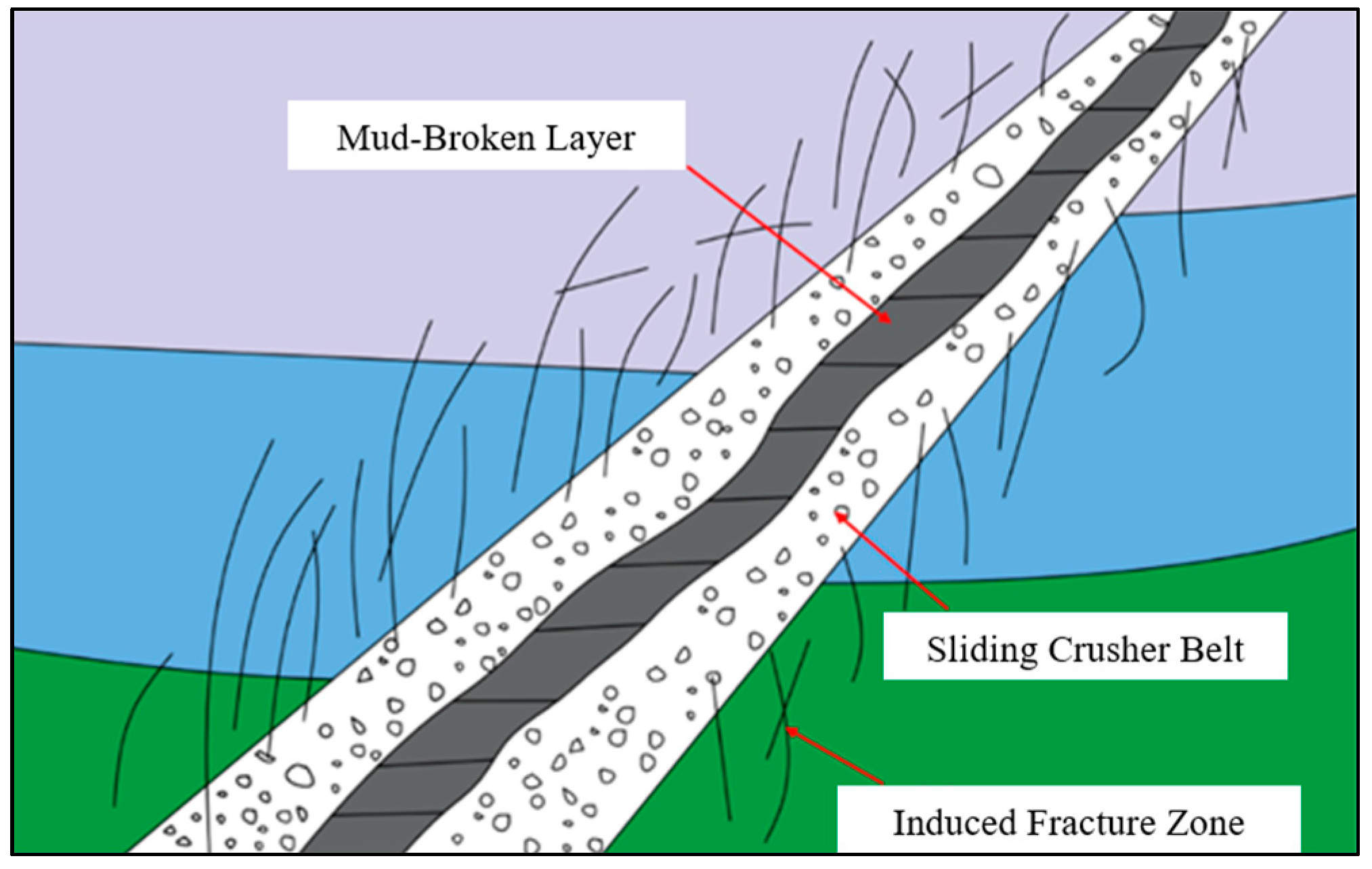
2.3. Characteristics of Reservoir Space in the Study Area

The main rock types of the lower sub-member of the 3rd member of Shahejie Formation reservoir in the study area are mudstone, siltstone, and sandy mudstone. The comprehensive analysis of the mud shale in the study area, utilizing a combination of X-ray diffraction (XRD), thin section microscopy, and scanning electron microscopy (SEM), provides detailed insights into its mineralogical composition and microstructural characteristics. The results indicate that the primary constituents of the mud shale are calcite and quartz, which form the fundamental framework of the rock. These minerals are commonly found in sedimentary environments and contribute significantly to the mechanical and physical properties of the shale. In addition to calcite and quartz, the mud shale also contains a variety of other minerals. Clay minerals, such as illite, kaolinite, and montmorillonite, are present and play a crucial role in determining the shale’s porosity and permeability. Dolomite, a carbonate mineral similar to calcite but with a higher magnesium content, is also identified. Potassium feldspar and plagioclase, both common silicate minerals, are found in smaller quantities. These minerals can influence the rock’s hardness and resistance to weathering. Minor amounts of pyrite and siderite are also detected. Pyrite, an iron sulfide mineral, can affect the redox conditions within the shale and may have implications for the presence of hydrocarbons. Siderite, an iron carbonate mineral, can contribute to the overall carbonate content of the rock. Other trace minerals may also be present, though in smaller quantities. Occasionally, the analysis reveals the presence of ostracods and phosphatic vertebrate fragments. Ostracods are small crustaceans whose fossilized shells can provide valuable information about the depositional environment and paleoecology of the area. Phosphatic vertebrate fragments, such as bone or tooth material, can offer insights into the faunal content and the conditions under which the sediments were deposited. Overall, this detailed mineralogical and microstructural analysis helps to characterize the mud shale’s composition and provides a foundation for understanding its geological history, physical properties, and potential for hydrocarbon storage and migration (Figure 3).
The types of reservoir space are classified into two main categories: pores and fractures. Pore types include intergranular micropores, intragranular pores, intramicropores, and dissolution pores; fracture types include bedding fractures, tectonic fractures, pressure fractures, and microfractures (Figure 4). Fractures can be further categorized into diagenetic fractures and tectonic fractures. Diagenetic fractures mainly include diagenetic bedding fractures and overpressure microfractures. The reservoir has undergone compaction and the precipitation and filling of authigenic minerals, leading to cementation of the rock and filling of fractures, resulting in relatively poor physical properties.

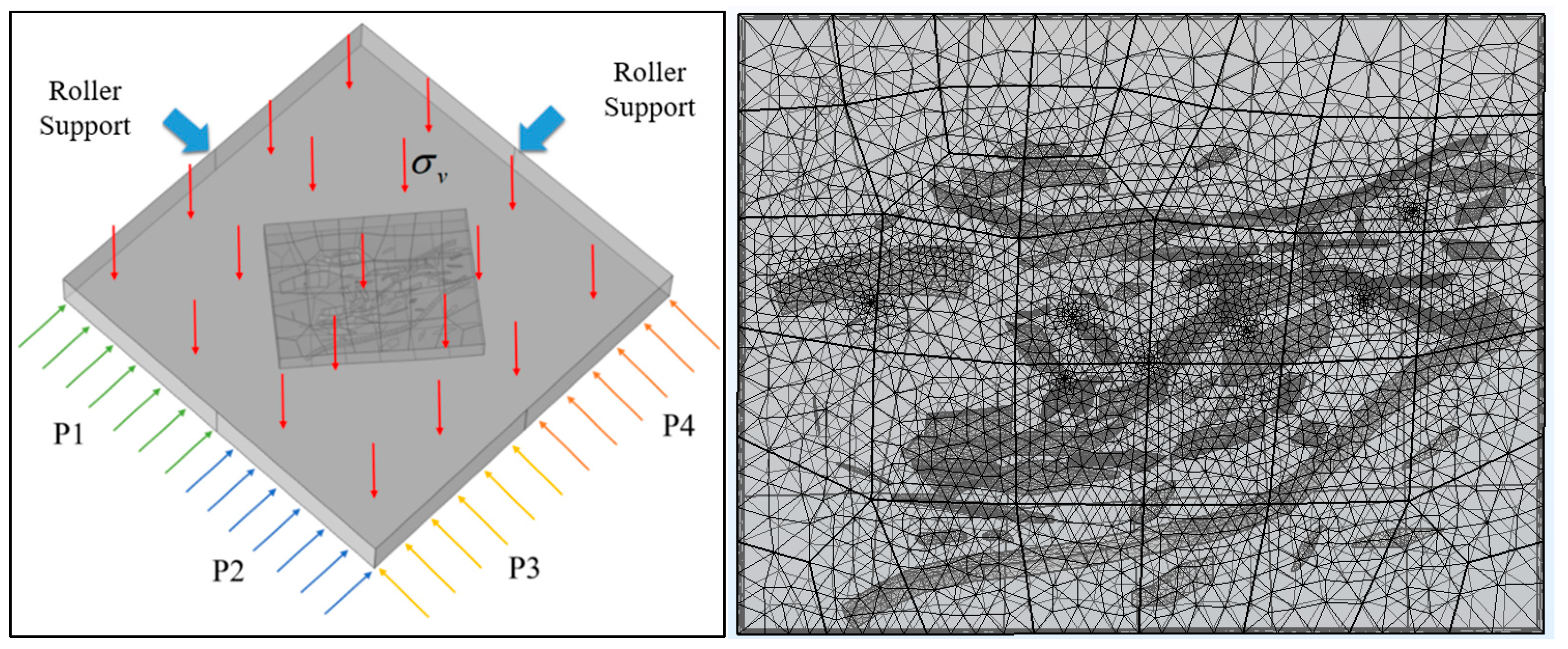
3. Geomechanical Modeling of Fault Fracture Body Reservoirs

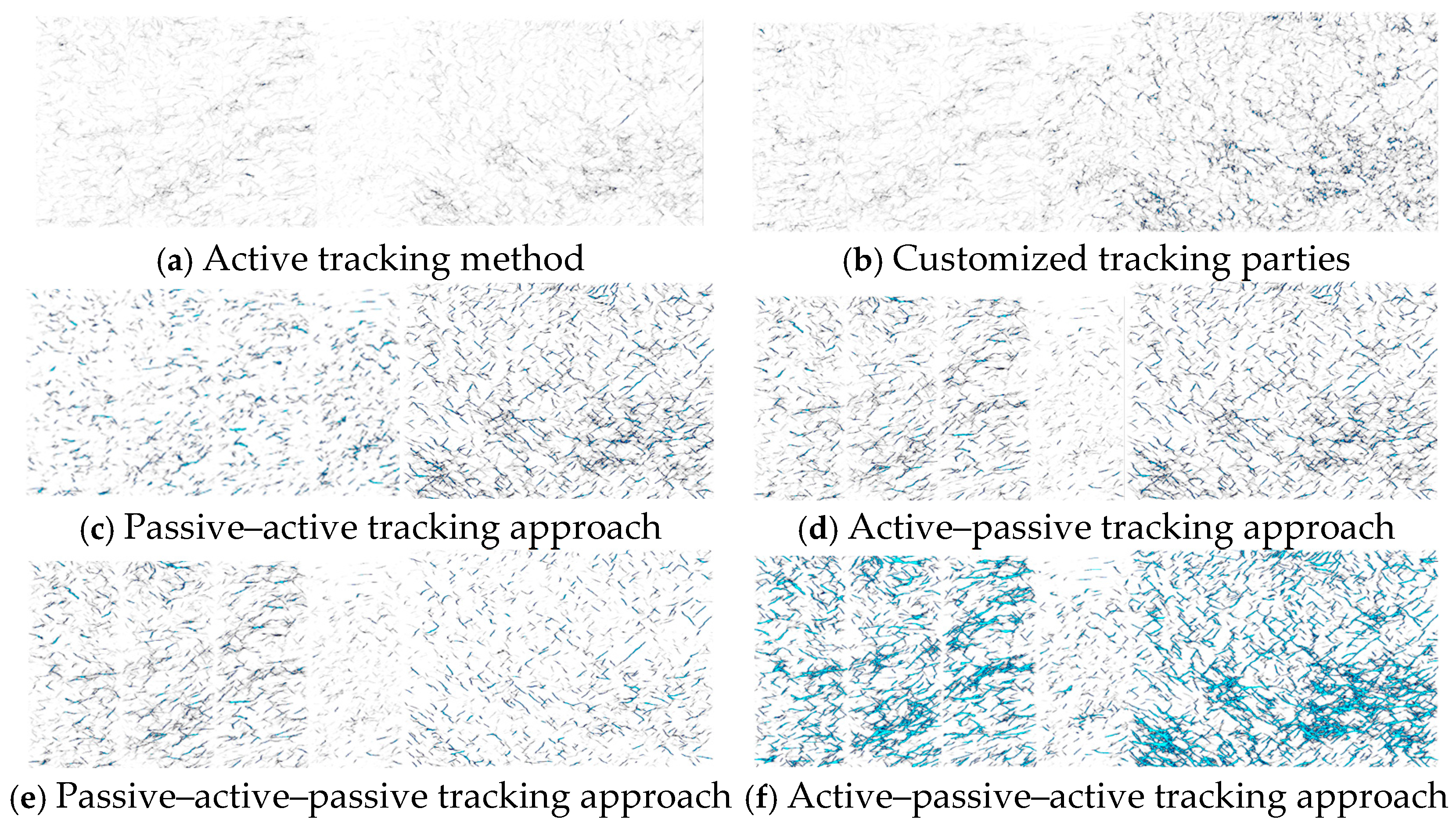
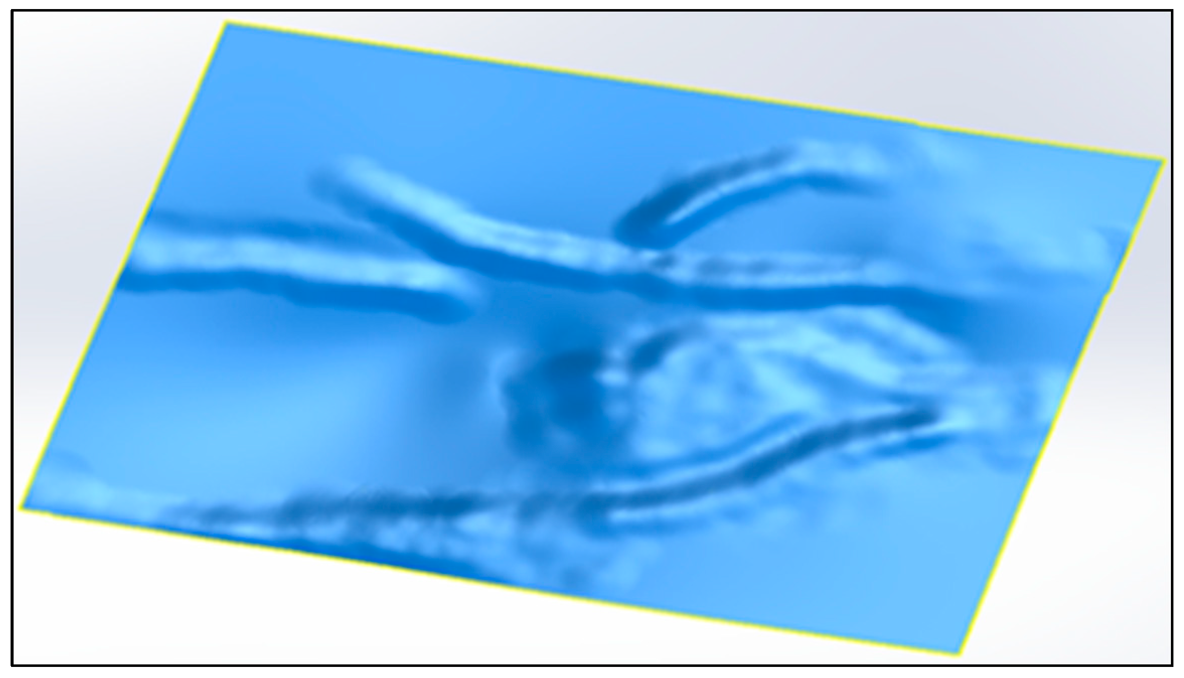
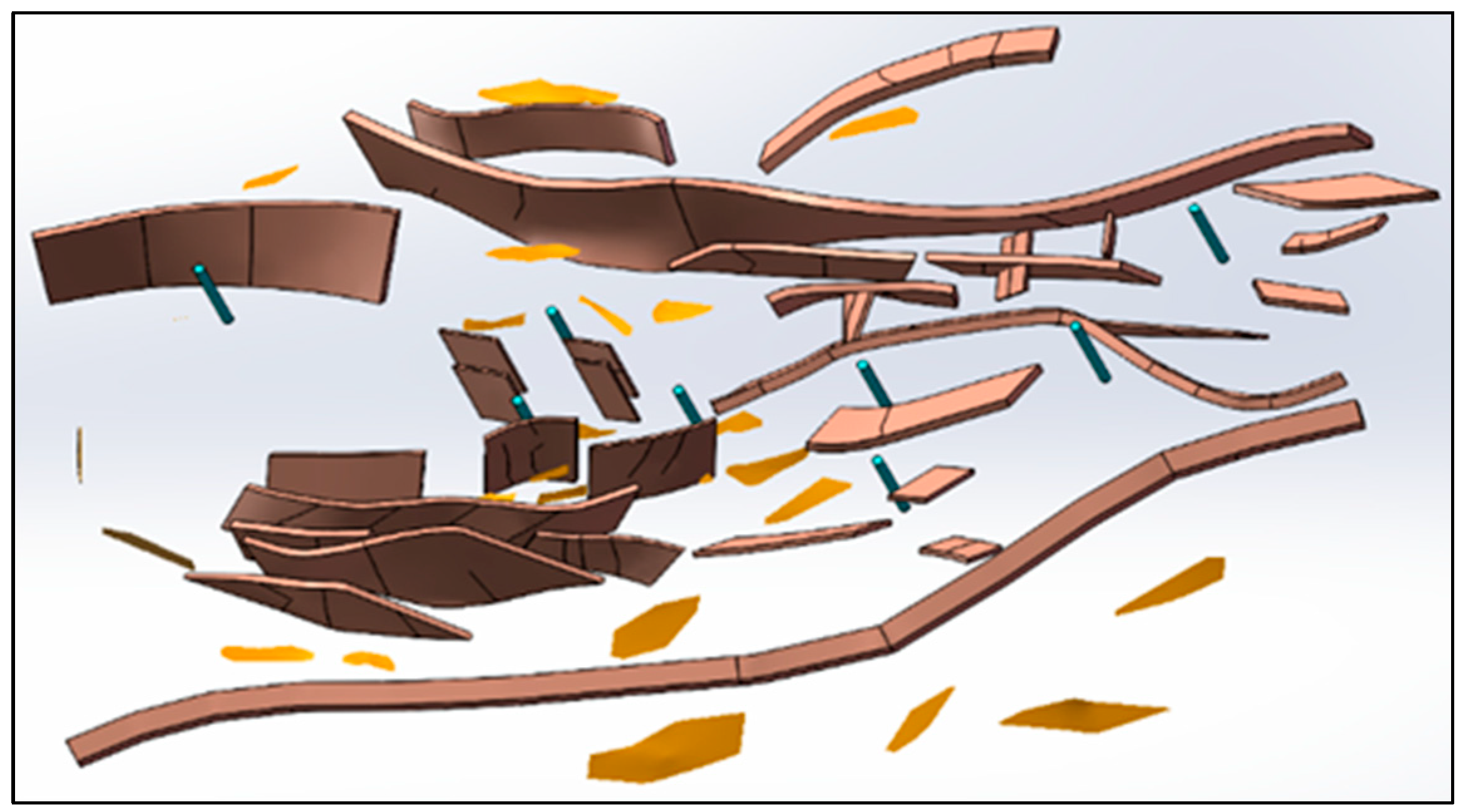
3.1. Skeleton Modeling of the Fault Fracture Body

Geological modelling, in terms of structure, sedimentological facies, and petrophysical properties, is an essential method for quantitatively understanding underground information. The main aim is to enhance the reliability of decision making for underground natural resource evaluation and recovery [20]. Geological modelling plays an important role for the work flow of gas/oil exploration and production. It provides a simulation pf the fundamental geological structures, sand body distributions, and petrophysical properties. Reserve volume calculations and dynamic reservoir simulation can be carried out based on the models [21]. The accuracy of these models depends on the techniques and methods used, and the reliability of the geological, well logging, and seismic data. Figure 5 shows that the middle and lower sub-member of the 3rd member of Shahejie Formation in the Jiangjiadian study area was developed using the well vibration combination method. This model provides valuable insights and understanding for reservoir analysis in the study area.
The Jiangjiadian study area exhibits complex geological structures, primarily influenced by numerous cross-faults, which are associated with the interaction of different fault systems and the resulting tectonic deformation. Properly managing the connectivity between these faults is crucial for ensuring high-quality meshing and accurate modeling. Individual adjustments were made to address this issue. Figure 6 illustrates the establishment of a new connection relationship between two faults, while fault-smoothing techniques were employed to enhance fault continuity. The fault model of the study area, once finally established, is shown in Figure 7.
After the establishment of the structural model, it becomes essential to ascertain the distribution of large natural fractures within the fracture system. These fractures typically develop near faults or other favorable tectonic sites and exhibit systematic variations in their development across different locations. First, an artificial intelligence technique called ant tracking is applied to generate an ant-tracking attribute cube. The ant-tracking attribute is the representation of the discontinuity in seismic data, and is often considered a good indicator for the existence of a natural fracture system [22,23,24]. In this study, automated ant-tracking technology was used to identify large natural cracks in the study area. The original seismic data undergoes a series of processing steps, including tectonic smoothing, boundary detection, boundary enhancement, and attribute extraction.
Three basic tracking methods (passive, active, and custom) were used to identify large natural cracks in the study area when using ant-tracking techniques. While passive and active tracking had fixed parameters, the customized method allowed for parameter adjustments based on specific situations. To enhance tracking accuracy, the ant body underwent multiple iterations based on previous results. The outcomes were comprehensively evaluated by comparing the effectiveness of various tracking methods, including active, customized, passive–active, active–passive, passive–active–passive, and active–passive–active. Details of the tracking parameter settings can be found in Table 1.
The initial boundary plays a pivotal role in determining the distribution of ants within the seismic body, influencing the overall distribution and computation time. The ant-tracking deviation restricts the degree to which ants can deflect. The ant step length permits ants to traverse a greater distance, albeit at a potential slight reduction in accuracy. The allowed illegal step length designates the maximum tracking distance in the absence of fracture information. The required legal step length establishes the number of steps necessary to identify valid fractures. The termination criterion is predicated on the percentage of illegal steps.
In this study, the effects of ant tracking under different methods were compared and analyzed. The seismic profiles of Xline 1188 and line1701 were taken as examples, as shown in Figure 8.
The color depth of the identification results and the spatial distribution of cracks indicate that the active–passive–active ant-tracking method is the most effective. This method furnishes a substantial amount of credible fracture information. Consequently, the results obtained from the active–passive–active ant-tracking method serve as the final crack recognition results and the basis for extracting the crack model. Figure 9 displays the extracted large natural fractures in the study area. The fracture model exhibits irregular facies sheets, which accurately represent the characteristics of fractures in real stratigraphic conditions. The fractures vary in direction and occurrence, spanning all layers. However, the majority of fractures are oriented in the NE direction, with a notable concentration of large fractures in the lower sub-member of the 3rd member of the Shahejie Formation.

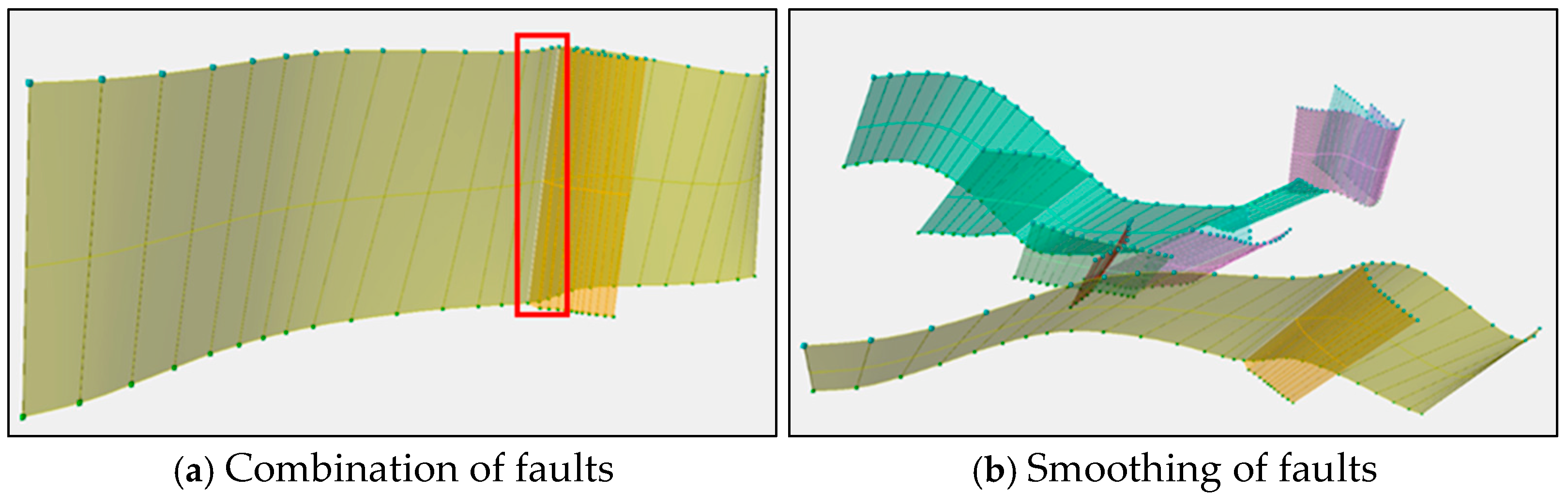
3.2. Principles of Fault Model Optimization

Previous studies and numerical simulations often simplified faults as simple surfaces, neglecting the complexity of real stratigraphic conditions. However, this approach does not capture the intricate structures observed in actual fractures. Figure 10 illustrates the internal architecture of the fault, which is composed of a fault mud at the core, a sliding fracture zone inundated with fractured rocks, and a peripherally located induced fracture zone exhibiting irregular development. The cracks identified through the ant-tracking technique include the large cracks within the induced fracture zone. Consequently, the subsequent optimization involves combining the fault mud with the sliding fracture zone, refining it as a new fault model based on the original fault surface. This process leads to the reconstruction of the fracture skeleton model as a fracture geomechanical model.

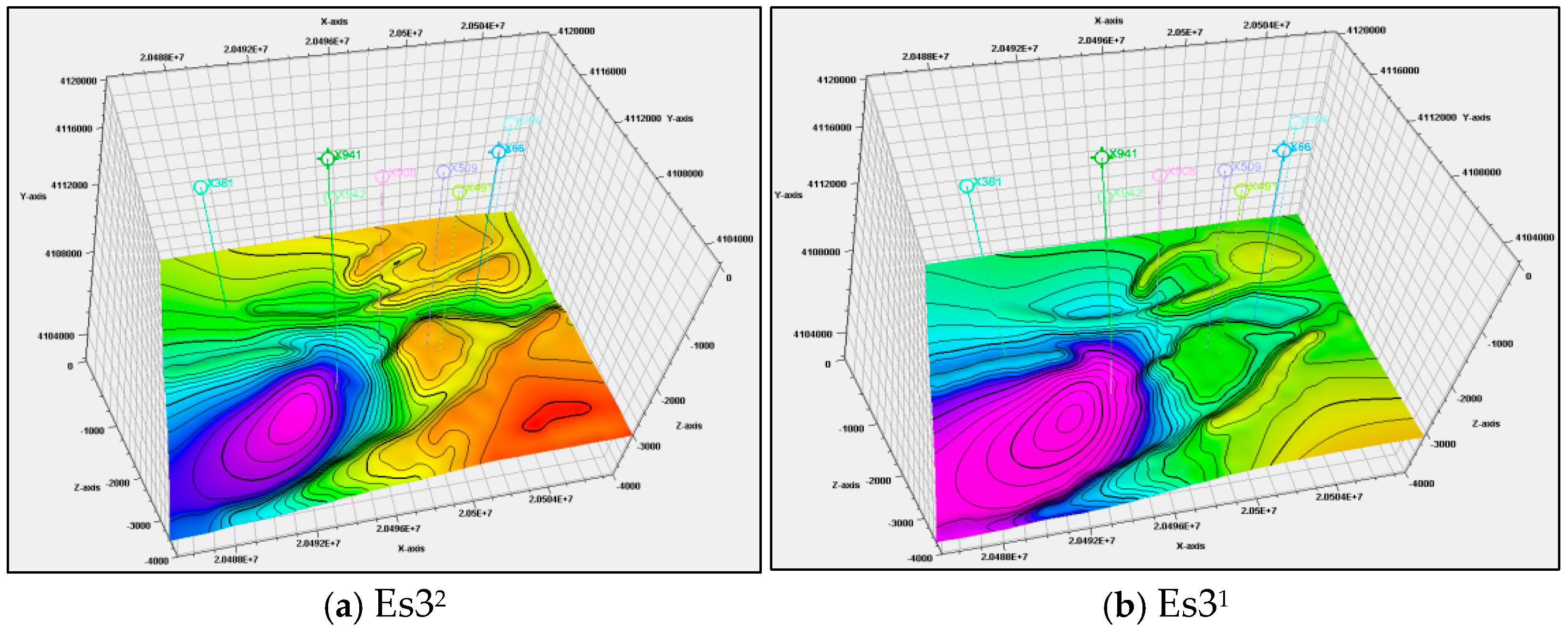
3.3. Inverse Reconstruction of Fault Fracture Body Reservoir Models

The Scan to 3D module in SolidWorks 2021 enables reverse modeling, commonly used in fine part design and 3D printing. By reconstructing the imported point cloud with the reverse function, reconstruction time is significantly reduced, and the model is restored to a high degree of accuracy. The established fault fracture body skeleton model is exported as extensive point clouds. Utilizing the Scan to 3D module, the fault surface model was reversely modeled and optimized, ensuring seamless integration between the 3D geological modeling software and the finite element software.
In order to restore the model information and achieve high precision reconstruction, it is necessary to optimize the point cloud through noise elimination and simplification. The segmentation of point cloud and the removal of points exceeding the average distribution are effective measures to eliminate noise. Simplification reduces the number of fixed points for grid features or overall data points, resulting in smaller and simpler files, and promoting effective mesh generation. However, excessive simplification risks sacrificing layer construction features. Thus, a 5% reduction control was applied while preserving original construction characteristics before mesh generation. Smoothing operations can be performed to address any imperfect or jagged areas in the mesh model (Figure 11).
It is important to use the inverse modeling method to generate the mesh model of the fractured reservoir and convert it into a surface. Enhanced surface details can maximize the recovery of local structural information. In order to simplify the subsequent finite element calculation, based on the fault distance of each fault in the study area, the fault plane model was successively optimized into the fault body model containing fault gouge and sliding fracture zone. Figure 12 depicts the resulting fault and lower sub-member of the 3rd member of the Shahejie Formation shale reservoir in the study area, obtained through reverse reconstruction.
In conducting numerical simulations of the in situ stress field within lower sub-member of the 3rd member of Shahejie Formation, it is imperative to apply appropriate seepage and mechanical boundaries to account for the coupling of seepage and stress. The boundary range of fracture fracture model of shale reservoir was expanded to reduce the local effect caused by boundary conditions. A novel transition zone was incorporated outside the pre-established model. The reservoir model within the area of study extended approximately 22.6 km by 16.8 km. A certain distance was extended in each horizontal direction to create the simulation transition zone. This established a geomechanical model of the fracture seam reservoir.

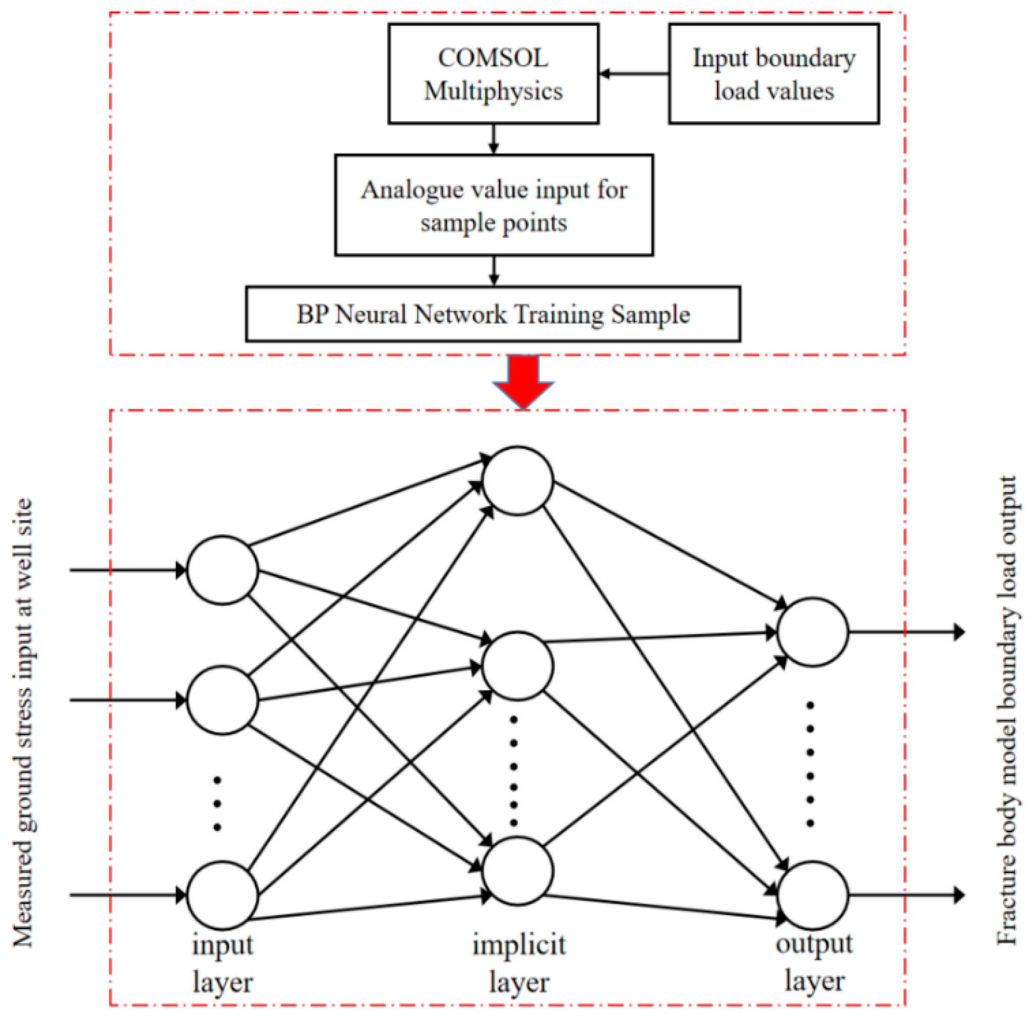
4. Machine Learning-Based Inversion of Boundary Conditions in the Study Area

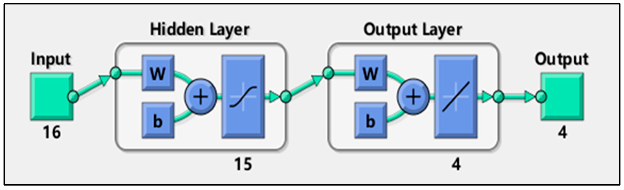
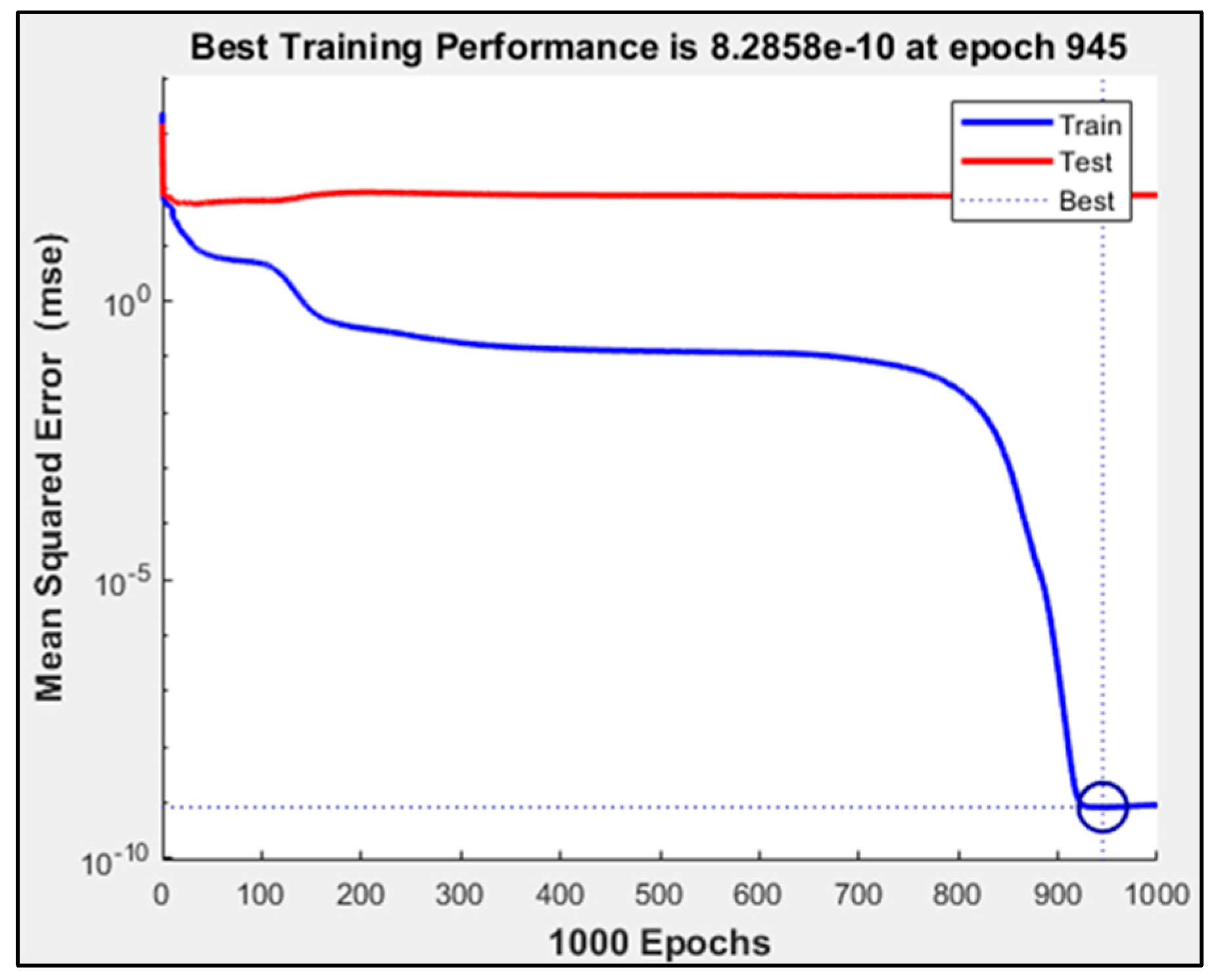
4.1. Principles of Machine Learning Model Prediction

In the geomechanical model, boundary conditions become requisite for the numerical simulation and analysis of the in situ stress field. Neural networks, particularly the BP neural network, are frequently employed for the inverse calculation of the initial stress field in complex geological environments. The BP neural network is a widely used multilayer feedforward network which has a powerful nonlinear mapping ability [25,26]. Because the stress and load in the actual formation are nonlinear, the BP neural network was used to invert the boundary conditions in the study area and determine the relationship between in situ stress and load.
Signal forward propagation and error backpropagation are essential aspects of BP neural networks. In a BP neural network model with one hidden layer, the operation can be divided into two stages. The first stage involves the forward propagation of signals, starting from the input layer, passing through the hidden layer, and reaching the output layer. The second stage consists of error backpropagation, starting from the output layer, passing through the hidden layer, and returning to the input layer. During this stage, the weights and biases are adjusted sequentially from the hidden layer to the output layer, and from the input layer to the hidden layer [27]. If n input samples and m output samples are set, the calculation formula of the output value of the hidden layer and the output value of the output layer is as follows:
x j = f i n W i j x i θ j
S k = f i = 1 p W i k x i θ k
where f ( x ) is the activation function, W i j is the weight from the input layer to the hidden layer. W i j is the weights from the hidden layer to the output layer, θ j is the threshold from the input layer to the hidden layer, θ k is the threshold from the hidden layer to the output layer, and p is the number of neurons in the hidden layer.
The error function defined to be used to reduce the total error is:
E = 1 2 l = 1 q k = 1 n Y k S k 2
where q is the total number of samples, Y k is the theoretical output value, and S k is the sample output value.
To minimize the total error, the gradient descent method adjusts the interlayer weights and thresholds during error signal backpropagation. In r iterations, the iterative formulas for the interlayer weights and thresholds of the hidden and output layers can be expressed as:
W i j r + 1 = W i j r + η Q = 1 q δ j Q x j Q
θ j r + 1 = θ j r + ξ Q = 1 q δ j Q
δ j Q = Q = 1 q Y j Q S j Q f ψ j Q
where η and ξ are scale factors, representing the learning rate; Q is the sample number, e.g., x j Q means the implicit layer output value obtained when Q samples are input x j ; and ψ j Q is the input value of the transfer function of the output layer.
The correction formula for the implicit layer weights and thresholds is:
Δ W i j = λ E W i j = λ Q = 1 q E Q S j Q S j Q x i j Q x i j Q W i j = λ Q = 1 q Y j Q S j Q W i j f φ j Q x j Q
Δ θ j = β E θ j = β Q = 1 q E Q S j Q S j Q x j Q x j Q θ j = β Q = 1 q Y j Q S j Q W i j f φ j Q
where λ and β are the step size, Q is the sample number, and ψ j Q is the hidden layer transfer function input value.

4.2. Inversion of Boundary Conditions

The process of determining the boundary conditions through machine learning consists of two stages: initial simulation and obtaining the in situ stress values at the well point by utilizing various initial boundary conditions. Subsequently, a BP neural network model was built and trained with these gathered samples. By introducing the in situ stress measured at the well point, the boundary load prediction value of the fracture model of shale reservoir was obtained. To handle computational complexity and time constraints, 30 sample groups comprising boundary load values were chosen as output samples. Preliminary simulations were conducted using finite element numerical simulation software to identify the maximum and minimum horizontal principal stresses at the wells in the study area. These stress values were employed as input samples for the neural network model (Figure 13).
In this study, a three-layer BP neural network model, comprising an input layer, a hidden layer, and an output layer, was employed. The input layer consisted of 16 nodes corresponding to the maximum and minimum horizontal principal stresses of eight wells in the study area. The hidden layer contained 15 nodes, while the output layer had 4 nodes corresponding to the boundary load values P1, P2, P3, and P4. Although the activation function was not explicitly specified, it is commonly a Sigmoid or Tanh function in BP neural networks. The network was trained using the error backpropagation algorithm and the gradient descent method. Thirty sets of sample data, obtained from preliminary simulations using finite element software, were used for training. The objective was to predict the boundary load values based on the in situ stress values at measurement points (Figure 14).
The neural network training error curve clearly indicates that the training error is already remarkably small and satisfies the specified target requirement by step 945 (Figure 15). In the neural network model used in this paper, the error value is expected to be relatively low, indicating good predictive performance. Specifically, the mean squared error (MSE) is estimated to be below 10 MPa², and the mean absolute error (MAE) is estimated to be below 3 MPa. These error values suggest that the model’s predictions are close to the actual boundary load values, with a high level of accuracy and reliability.
The maximum and minimum horizontal principal stresses at 3500 m depth for each well measurement point were used as input values for the BP neural network prediction model. The input parameters ranged from 53.23 MPa to 79.86 MPa for the maximum horizontal principal stress and from 46.59 MPa to 68.79 MPa for the minimum horizontal principal stress. The output parameters, which were the boundary load values, were determined to be 62.69 MPa for P1, 78.02 MPa for P2, 78.47 MPa for P3, and 64.18 MPa for P4 (Table 2). The accuracy of the neural network model in predicting boundary loads of the shale reservoir fracture model was validated by comparing its predictions with the results obtained from numerical analysis. The results demonstrate that the neural network model exhibits high accuracy in predicting boundary loads, showing good consistency with the numerical analysis results [28].

5. Three-Dimensional In Situ Stress Field Distribution of Fracture Reservoirs

5.1. Coupled Flow–Solid Control Equations

During reservoir extraction, the weight of the rock is borne by the rock skeleton and the pore fluid. Groundwater within the reservoir affects the mechanical properties of the natural rock mass. The continuous exploitation of resources leads to the seepage of underground fluids and changes in pore pressure, which affect the distribution of effective stress and the stress field of the fractured rock mass skeleton, thereby influencing the flow of pore fluid and pressure distribution [29]. The change in the rock skeleton caused by seepage requires the calculation of the stress field equation to be based on the assumption that the solid phase of reservoir is a kind of elastic medium with slight deformation. These equations can be derived from fundamental relationships of elastic media [30,31]. Assuming the rock mass as an ideal elastic body, the stress components within it can be expressed as follows:
σ i j = 2 G ε i j + λ ε v δ i j + α P δ i j
where G is the shear modulus, GPa, ε i j is the strain component, λ is the Lamey constant, ε v is the strain, δ i j is the Kronecker number (1 for i = j and 0 for i j ), α is the Biot coefficient, and P is the pore water pressure, GPa.
The static equilibrium equations are:
σ i j , j + F i = 0
The effective stress equation is:
σ i j = σ i j + P δ i j
The stress field control equation is obtained by joining the above equations as:
G 2 u + ( λ + G ) x ( u x + v y + w z ) α P x = F x G 2 u + ( λ + G ) y ( u x + v y + w z ) α P y = F y G 2 u + ( λ + G ) z ( u x + v y + w z ) α P z = F z
where u, v, and w are the displacements in the x, y, and z directions, respectively, and Fx, Fy, and Fz are the volumetric forces in the x, y, and z directions, respectively.
Under the action of fluid–structure coupling, the differential equations related to fluid pressure and rock skeleton displacement are obtained after eliminating the irrelevant variables of the fluid continuity equation, state equation, and Darcy’s law [32,33,34,35].
The Darcy equation is:
V = ϕ v r = κ μ P + ρ w g Z
where V is the seepage velocity of the fluid, cm·s−1, ϕ is the rock porosity, μ is the hydrodynamic viscosity, Pa·S, and κ is the permeability tensor, m2.
The fluid and rock skeleton continuity equations are combined to form the overall continuity equation under seepage–stress coupling:
ϕ ρ w t + ρ w ε v t + 1 ϕ ρ w ρ s ρ s t + · ρ w ϕ v r = ρ w q
where q is the mass source, kg/(m3·s), ρ s is the rock skeleton density, kg·m−3, ρ w is the fluid density, kg·m−3, and ε v is the rock skeleton strain.
The change in the density of the rock skeleton under flow–solid coupling can be expressed as:
ρ s = ρ s 1 + P P 0 K m t r σ σ 0 1 ϕ 3 K m
where ρ s is the rock skeleton density, kg·m−3, ρ s is the initial value of rock skeleton density, kg·m−3, K m is the rock skeleton bulk modulus, GPa, and σ σ 0 is the effective stress tensor, GPa.
After deriving the Darcy equation and incorporating the equation describing the relationship between the rock skeleton density and time, the overall continuity equation is formed under flow–solid coupling:
α ε v t + α ϕ K m + c w ϕ p t + · κ μ · P + ρ w g Z = ρ w q
where α = 1 K / K m is the effective stress coefficient, ρ w = ρ w 1 + c w P P 0   ρ w is the initial density of fluid, kg·m−3, and cw is the fluid compression factor, Pa−1.

5.2. Model Parameter Setting

The numerical simulation model of the fracture reservoir in the study area, under fluid–solid coupling, has an internal size of 22.6 km by 16.8 km and an overall model size of 45 km by 45 km, representing the real thickness of the study section. The inversion-derived boundary load values (P1 = 62.69 MPa, P2 = 78.02 MPa, P3 = 78.47 MPa, P4 = 64.18 MPa) are applied as mechanical boundary conditions. The model has fixed-constrained roll supports on the bottom and the other two sides, with a vertical upward stratum pressure of 80 MPa. In the model, the influence of distant fluid on the seepage field in the study area is ignored as there are impervious boundaries around it, and the pressure near the wellhead is 1.5 MPa (Figure 16). Key parameters for numerical simulation of shale reservoir fracture bodies are summarized in Table 3. The validation was conducted by comparing the maximum and minimum horizontal principal stresses calculated by the numerical model with those obtained from existing analytical formulas. The results demonstrate a good consistency between the numerical model and the analytical formulas, indicating that the numerical model is capable of accurately calculating the in situ stress. This validation ensures the accuracy and applicability of the model in simulating the three-dimensional in situ stress distribution in the reservoir [36].

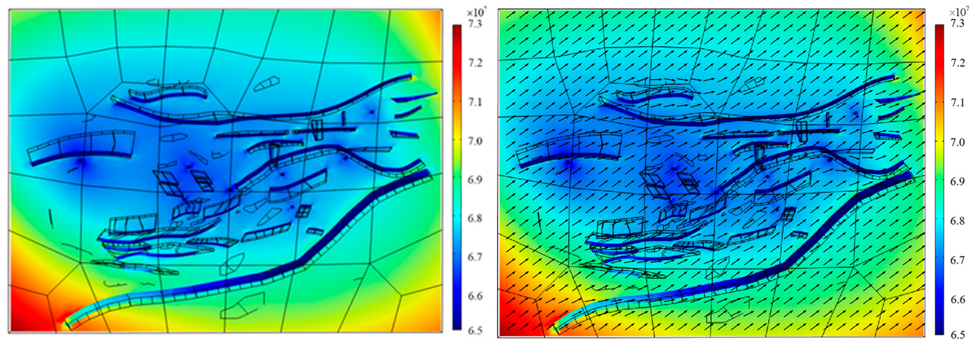
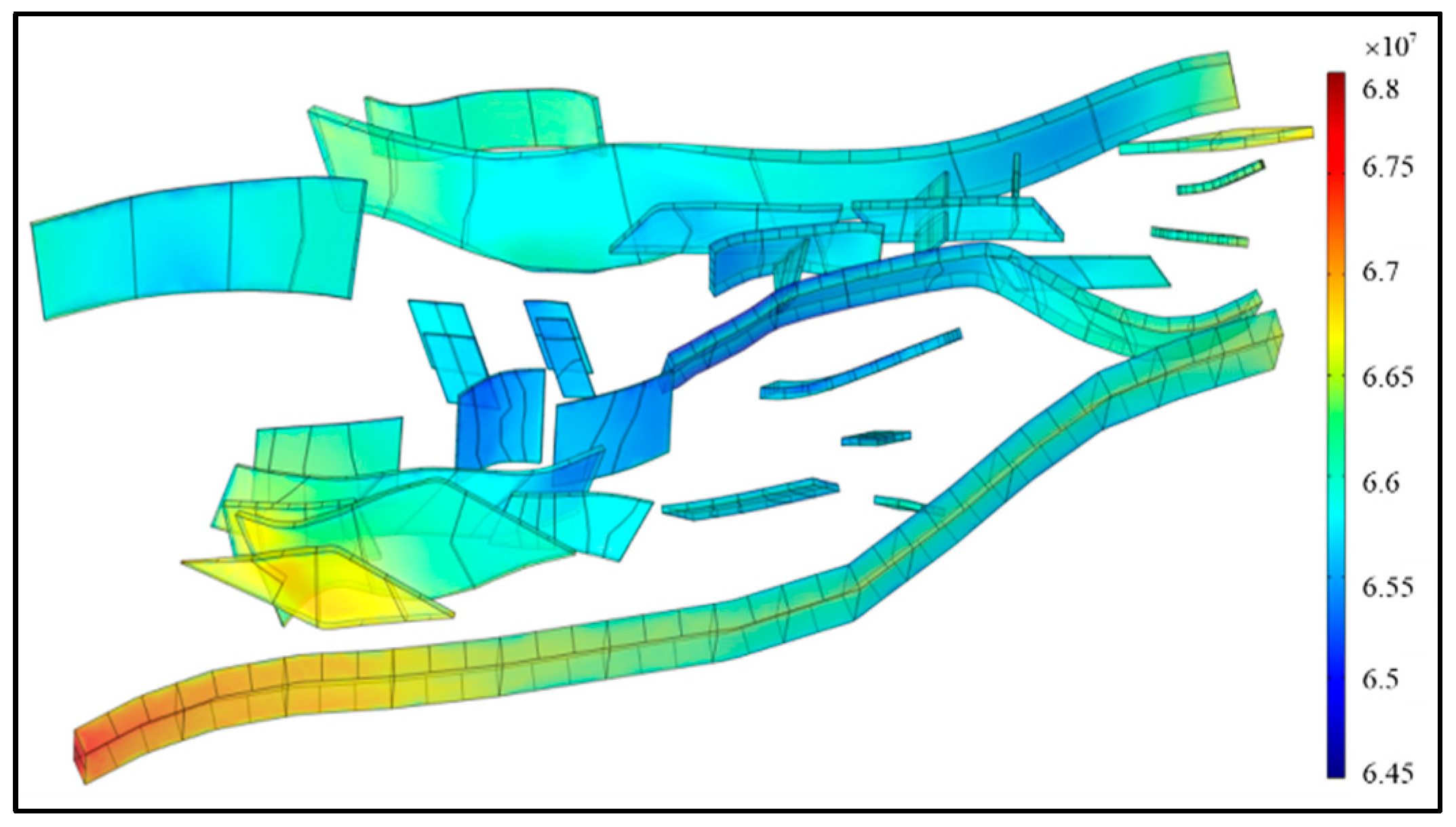
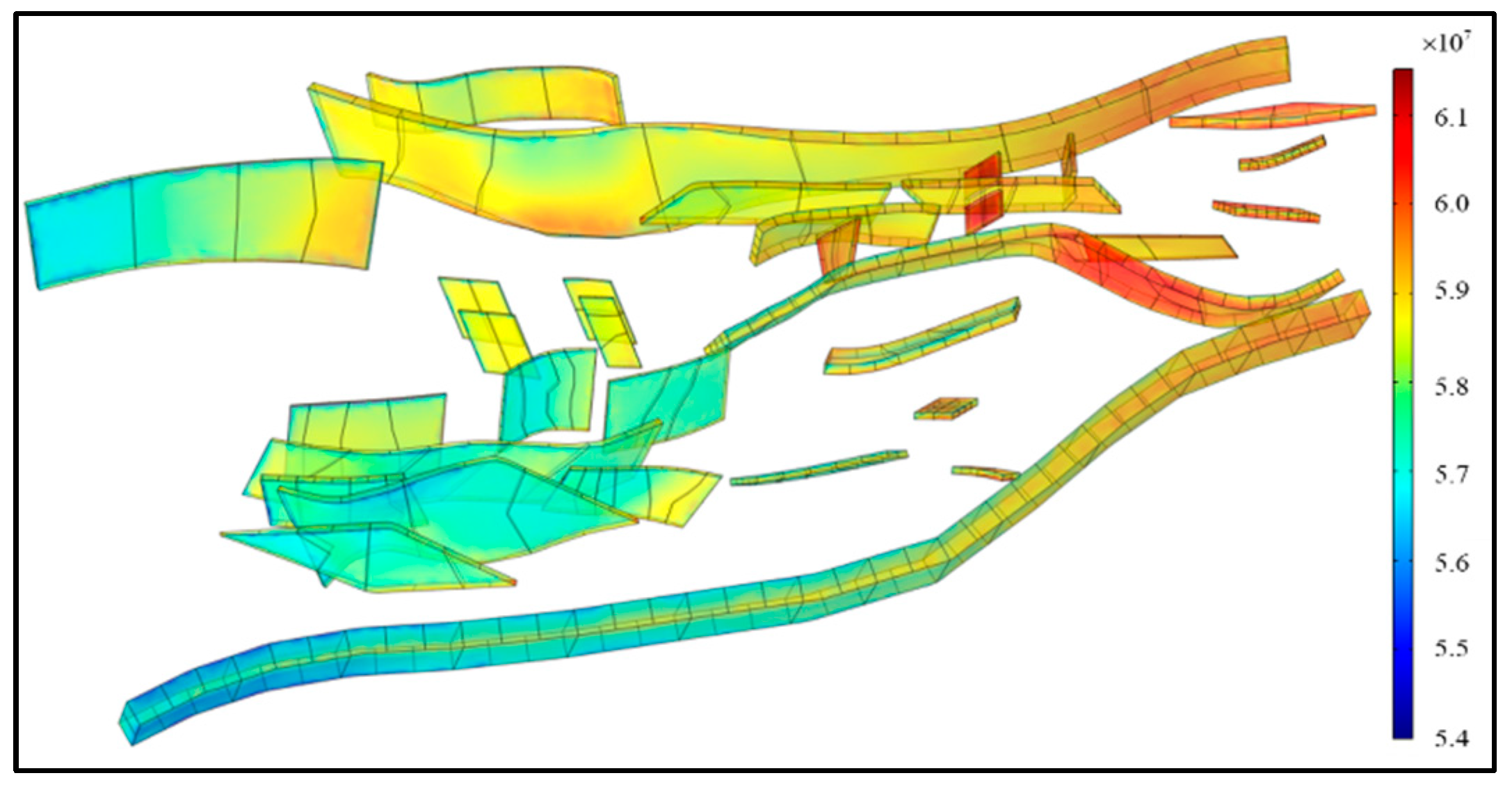
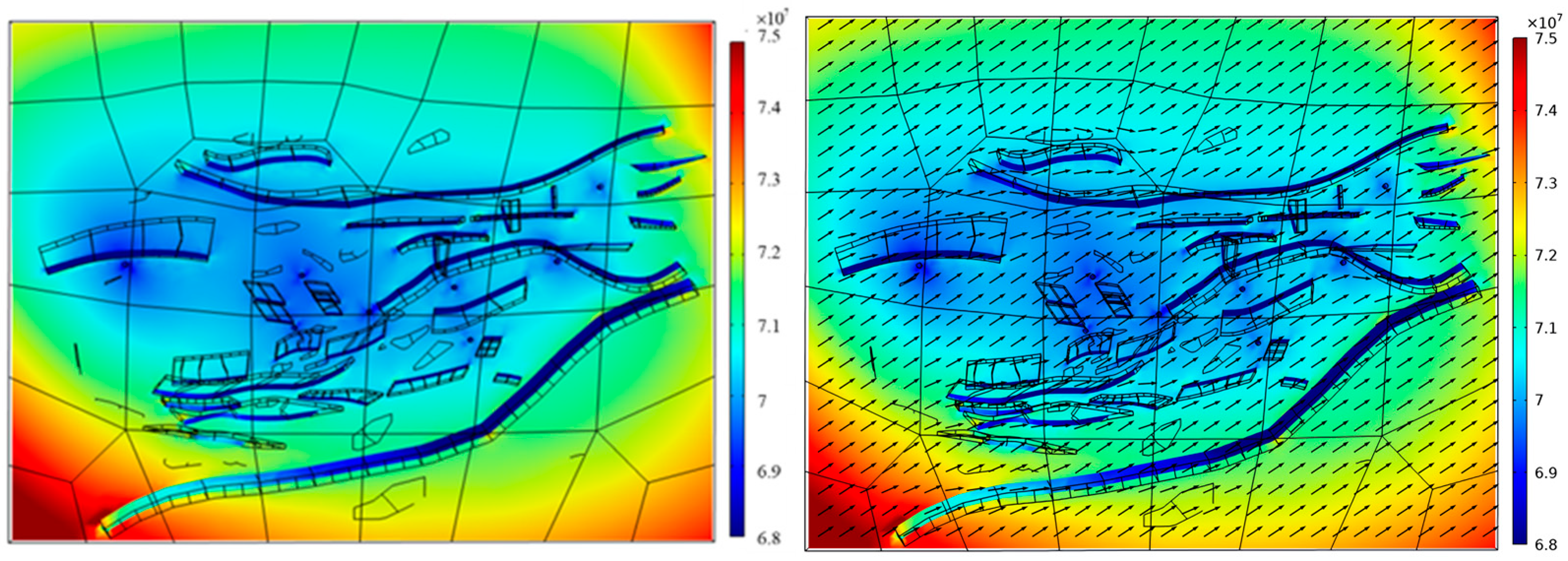
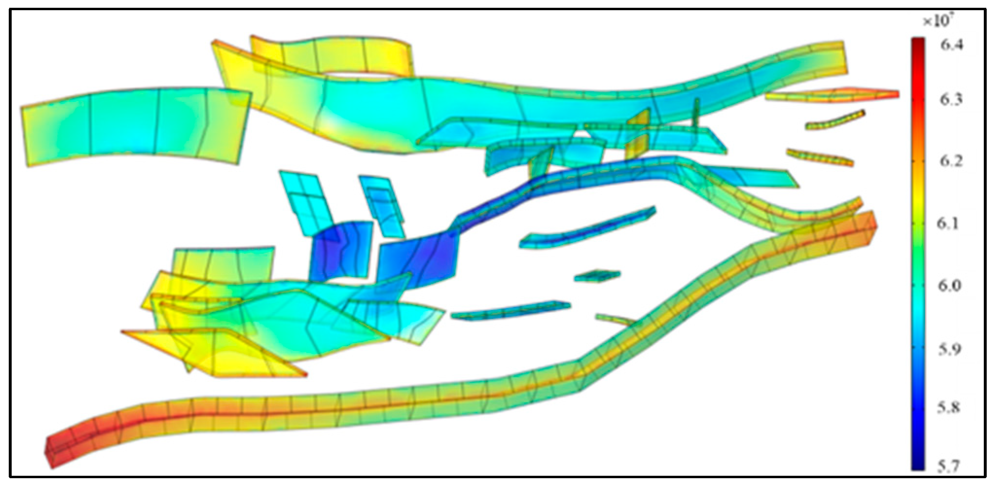
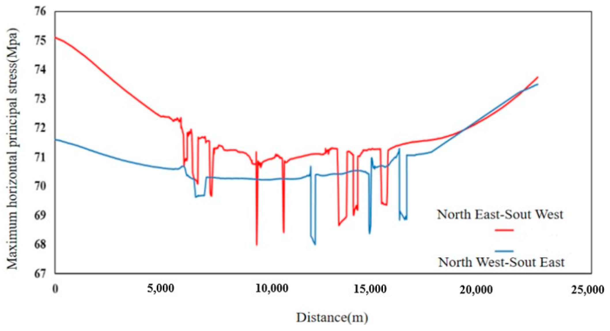
5.3. Study of Stress Field Distribution in the Area Without Considering Fluid Flow Coupling Effects

To facilitate comparative analysis, a numerical simulation of the stress field in the fault fracture body was first conducted without considering the fluid–solid coupling effects. Figure 17 and Figure 18 show the distribution and orientation of the maximum and minimum horizontal principal stresses in the fault fracture body of the shale reservoir at a depth of 3500 m.
As shown in Figure 17, under the condition without considering fluid–solid coupling effects, the maximum horizontal principal stress in the fault fracture body region of the study area ranges from 65.2 to 70.0 MPa. The maximum horizontal principal stress is relatively lower in areas with a dense distribution of faults and fractures, concentrating around 65.2–68.5 MPa. Stress concentration is observed at the southwestern end of the fault fracture body model, where the maximum horizontal principal stress is higher, ranging from 70.0 to 72.7 MPa. Additionally, the stress values within the faults are significantly lower than those in the surrounding areas, and the maximum horizontal principal stress near the faults is also lower than that in typical matrix regions. Under the influence of a single stress condition, the direction of the maximum horizontal principal stress in the fault fracture body region is 45° northeast. The overall trend of variation is not obvious; however, near the faults, the direction experiences deflection. Within a certain range, the larger the fault size, the greater the deflection angle.
Figure 18 shows that under the condition without considering fluid–solid coupling effects, the minimum horizontal principal stress in the fault fracture body region of the study area ranges from 57.5 to 62.0 MPa. The minimum horizontal principal stress is relatively lower in areas with a dense distribution of faults and fractures, concentrating between 57.5 and 61.2 MPa. The minimum horizontal principal stress is higher at the northwest and southeast ends of the fault fracture body model, with values ranging from 62.0 to 63.8 MPa. A significant decrease in the minimum horizontal principal stress is observed within the faults, and stress concentration occurs at both ends of the faults. Under a single stress condition, the direction of the minimum horizontal principal stress in the fault fracture body region is 45° southeast, with deflection occurring near the faults, particularly at the location of the Xiakou major fault where the deflection is more pronounced.
Faults are an important component of the fault fracture body and serve as crucial channels for oil and gas migration within the reservoir. To more clearly illustrate the stress variation within the fault in the fault fracture body structure, the fault model is displayed separately. The distribution of the maximum horizontal principal stress under the influence of stress is shown in Figure 19, and the distribution of the minimum horizontal principal stress is shown in Figure 20.
As shown in Figure 19 and Figure 20, under the condition without considering fluid–solid coupling effects, the maximum horizontal principal stress within the faults of the fault fracture body of the study area ranges from 65.2 to 67.5 MPa, while the minimum horizontal principal stress ranges from 56.8 to 61.0 MPa. Stress discontinuities occur at the fault ends and their connecting areas, with more pronounced stress variations observed at the Xiakou major fault.

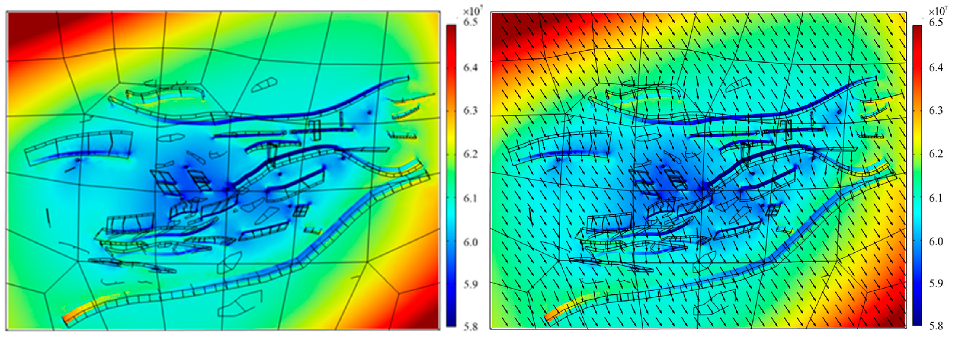
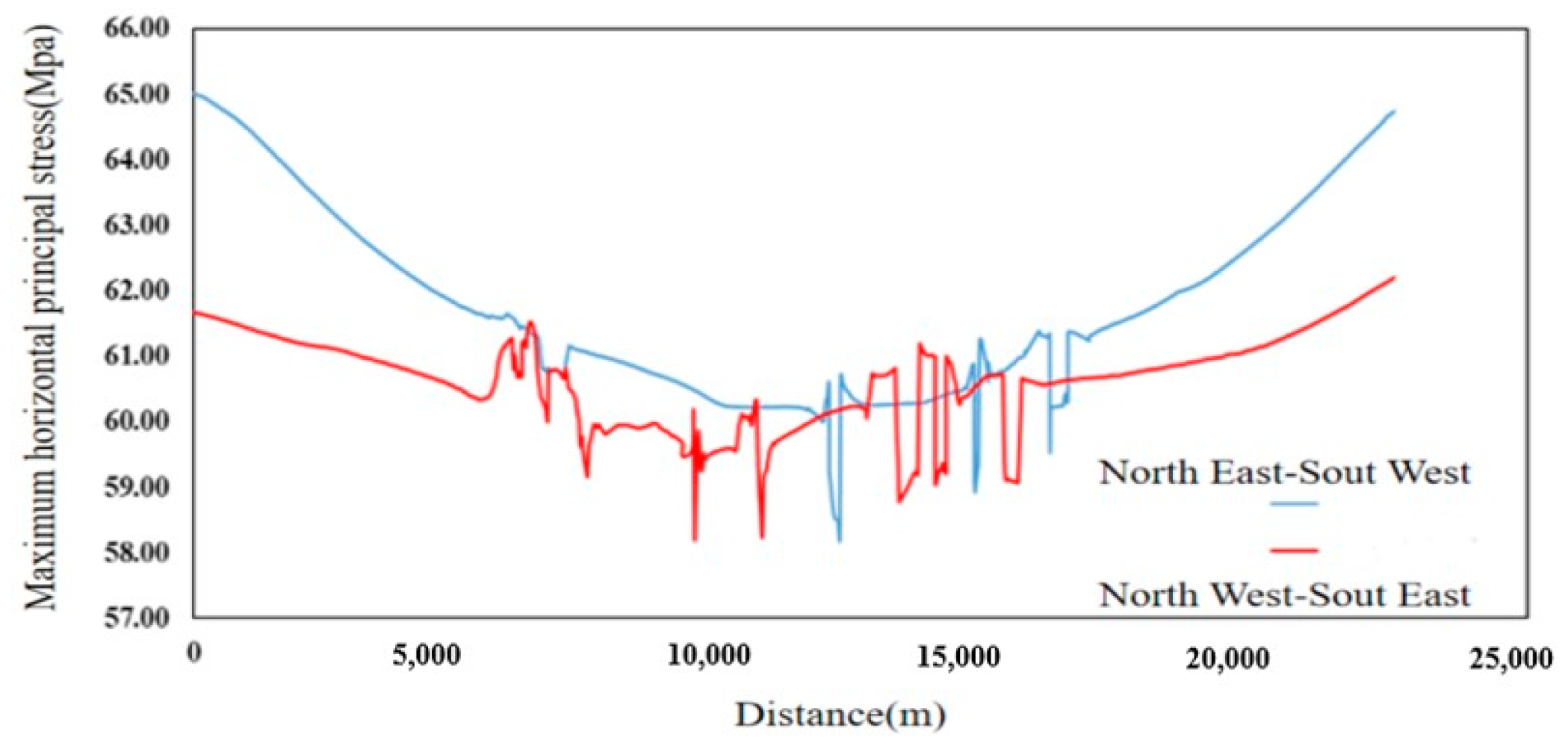
5.4. Analysis of In Situ Stress Field Characteristics in the Fault Fracture Body Reservoir Under Fluid–Solid Coupling Effects

The geomechanical model and governing equation of the fractured reservoir were used to simulate the in situ stress distribution of fractured reservoir. In this section, the distribution of the maximum and minimum horizontal principal stresses at the depth of 3500 m is analyzed in combination with the direction diagram.
Under fluid–solid coupling, the maximum horizontal principal stress in the fracture area of the Jiangjiadian region is from 68.2 to 72.8 MPa, indicating a compressive stress state. The maximum stress is lower in the middle of the model with dense faults and fractures, and higher in the southwest and northeast, with a distribution range of 72.7~72.8 MPa. Stresses at cracks are slightly lower than those in the surrounding substrate. The maximum horizontal principal stress inside the fault is lower than that outside the fault. The stress value at the ends of the fault is greater than in the middle, and the maximum horizontal principal stress inside the fault gradually increases from the middle towards both ends.
The maximum horizontal principal stresses in the fault body of the study area predominantly align in the northeast direction. Specifically, the direction of the maximum stresses at the center of the fault is approximately 48° northeast. Moving from the central region towards the peripheral area, the direction of the maximum stress progressively veers northward in the southwest and northeast directions, whereas it tends to divert eastward in other directions. The local deviation of the maximum stress direction inside the fault is obvious and perpendicular to the fault, and the deflection of the Xiakou fault is more obvious (Figure 21).
Under fluid–solid coupling, the minimum horizontal principal stress in the fracture area of the Jiangjiadian region is from 58.2 to 63.1 MPa, indicating a compressive stress state. The zoning effect of the minimum horizontal principal stress distribution is prominent, with lower stress values concentrated in the central part of the seam model (58.2–60.9 MPa) compared to other areas. Significantly, the stress values at the northwestern and southeastern termini of the seam model exhibit a substantial increase (62.7–65.0 MPa). The density of the large fracture system leads to the decrease in the stress value of the coal seam reservoir (Figure 22).
The lower stress values observed at the cracks and inside faults compared to the surrounding areas can be attributed to the mechanical properties of fault gouges and fractured rocks, which are softer and more compliant than the intact rock matrix. This allows for easier deformation and stress relaxation within these zones. Additionally, stress redistribution mechanisms, such as the stress shadow effect near fault tips and fracture edges, lead to lower stress concentrations within these zones. The influence of fluid pressure, which can counteract applied stress and reduce effective stress, is particularly significant in deepwater environments with low-porosity and low-permeability reservoirs. These findings are applicable in geological settings characterized by complex fault systems and significant fluid–solid coupling effects, such as those found in the Linnan Sag of the Bohai Bay Basin.
The minimum horizontal principal stress in the fault of the study area generally trends southeastward and is perpendicular to the direction of the maximum horizontal principal stress. Specifically, at the central region of the fault, the minimum horizontal principal stress is approximately 42° southeast. From the central region to the outer region, the direction of the maximum horizontal principal stress in the northwest and southeast gradually deflects to the south, and the other directions deflect to the east. Within the fault, the direction of the minimum horizontal principal stress experiences local diversion, aligning more parallel to the direction of the fault strike.
To analyze the variation of fault in situ stress in the fracture-seam reservoir of the study area under the influence of fluid–solid coupling, a separate fault model was presented (Figure 23 and Figure 24).
Under fluid–solid coupling, the faults exhibit maximum horizontal principal stresses from approximately 68.2 MPa to 72.5 MPa, and concentrated minimum horizontal principal stresses within the range of 58.0 MPa to 63.1 MPa. The stress value increases slightly in areas with dense fault distribution. The stress concentration is more pronounced at the end of the fault, and there are abrupt changes along the connecting fault, although the change is smaller than under a single stress condition. Similarly, the stress value at the fault junction is less than the sudden change under single stress condition.
Under the action of fluid–structure coupling, the complex structure inside the fracture body leads to the obvious zoning of the reservoir in situ stress field. The maximum and minimum horizontal principal stress distribution curves in the NE–SW and NW–SE directions of the model are plotted respectively in Figure 25 and Figure 26.
The fracture-seam reservoir in the study area exhibits a relatively low maximum horizontal principal stress in the northwest–southeast direction. Significantly, the stress value in the northwest region is markedly lower in comparison to the remainder of the area. Furthermore, the stress distribution curve at the southeast end bears a close resemblance to the stress distribution curve running from northeast to southwest. The overall zonation distribution of fractures is obvious, and the maximum horizontal principal stress decreases along the fracture development area. The stress concentration at the northeast and southwest ends is consistent with the nephogram.
Faults and fractures significantly influence stress distribution in geological formations by serving as pathways for fluid flow and impacting hydrocarbon accumulation. This influence arises from their lower mechanical strength and rigidity compared to the surrounding intact rock, which allows for easier deformation and localized stress reductions. Additionally, the higher permeability of fractures facilitates fluid migration, altering effective stress in the surrounding rock. Stress tends to concentrate at the tips of fractures and edges of faults, creating local anomalies and stress shadow effects. The presence of complex fault systems and deepwater depositional environments further enhances these dynamics, particularly in low-porosity and low-permeability reservoirs. Moreover, the interaction between fluid flow and rock deformation, known as fluid–solid coupling, plays a critical role in modifying pore pressures and stress states. Understanding these factors is essential for optimizing hydrocarbon exploration and production strategies.
Within the fracture seam of shale reservoirs in the study area, the minimum horizontal principal stresses in the northeast–southwest direction are generally reduced. The stress curves in both the northwest-southeast and northeast–southwest directions exhibit substantial decreases due to the extensive development of faults and fissures in the central region of the fracture seam. There is no significant difference between the stress values in these two directions. In the four corner regions along the diagonal, the minimum horizontal principal stresses in the northeast–southwest direction are less than those in the northwest–southeast direction, which is in line with the zoning characteristics demonstrated in the cloud diagram of the minimum horizontal principal stress distribution. The subarea characteristics of the in situ stress field, with significant decreases when traversing fault fractures and stress concentration at fault ends, are primarily due to the mechanical properties of faults and fractures, which have lower strength and rigidity compared to the surrounding rock, leading to localized stress reductions. Stress is redistributed due to the complex geometry and orientation of faults, causing deflection and concentration of stress directions at fault ends. Additionally, fluid–solid coupling effects, where fluid pressure within faults counteracts applied stress, further influence the stress distribution. These factors collectively create the observed stress patterns in the geological formation.
This study integrates geological, logging, and seismic data and employs advanced ant-tracking techniques to establish a skeletal model of the fault fracture body, providing a detailed three-dimensional view of the geological structure of the study area. This detailed structural model enables researchers to more accurately identify and locate fracture systems, which is crucial for understanding the mechanisms of hydrocarbon storage and flow. Furthermore, the model considers fluid–structure coupling and uses finite element numerical simulation software to simulate the three-dimensional in situ stress field of the reservoir. This simulation not only provides stress values at different stratigraphic levels but also reveals the distribution characteristics of the stress field within faults and fractures, which is of significant guiding importance for optimizing well placement and fracturing operations. Additionally, this study employs machine learning techniques to invert the boundary conditions of the study area, further enhancing the accuracy and reliability of the simulations. The research provides an in-depth analysis of how faults and fractures affect the in situ stress field and how these geological structures influence the distribution and extraction efficiency of hydrocarbons. Therefore, this study not only offers important technical support for hydrocarbon exploration and development in the Linnan Sag but also provides valuable theoretical references for the development of oil and gas fields under similar geological conditions.
Although machine learning algorithms and numerical simulation methods possess significant advantages in investigating the three-dimensional in situ stress distribution in the shale reservoir of the Linnan Sag in the Bohai Bay Basin, these approaches are also subject to certain limitations. Machine learning algorithms demand high data quality and quantity, suffer from insufficient model interpretability, are prone to overfitting, and entail substantial computational resources and time costs. Numerical simulation methods, on the other hand, may result in discrepancies between simulated outcomes and actual conditions due to model simplifications, uncertainties in boundary conditions, computational accuracy, mesh discretization, and limitations of the fluid–solid coupling theory. Moreover, the integration of these two methods requires interdisciplinary knowledge and skills, and there is a lack of sufficient independent validation data to comprehensively verify the accuracy of the models.

6. Conclusions

This study provides a comprehensive analysis of the shale reservoir fracture system in the Linnan Sag by integrating geological, logging, and seismic data with advanced techniques such as ant tracking. The distribution characteristics of the in situ stress field were analyzed, offering new technical strategies and theoretical support for well renovation and improving reservoir development efficiency. These findings contribute to advancing the understanding and optimization of reservoir management in similar geological settings. The following conclusions can be drawn:
(1) According to the different seismic data, different tracking methods were used to identify natural fractures, and it is found that the active–passive–active tracking method was the most effective in the identification of fractures. The fracture models in the study section exhibited spatially irregular facets, primarily concentrated near the faults, with a predominant distribution at the Xiakou large fault and the Jiangjiadian oil field strike-slip fault cluster.
(2) The BP neural network prediction model was established using the machine learning method to realize the inversion of boundary conditions. Finally, the boundary load of the fracture geomechanical model of the shale reservoir was obtained by using the BP neural network after training. The calculated loads for P1, P2, P3, and P4 were 62.69 MPa, 78.02 MPa, 78.47 MPa, and 64.18 MPa, respectively.
(3) Under the fluid–solid coupling conditions, the maximum horizontal principal stresses within the fracture reservoir of the study area varied between 68.2 and 72.8 MPa, whereas the minimum horizontal principal stresses ranged from 58.2 to 63.1 MPa. The distribution of the in situ stress field within the fracture displayed pronounced subarea characteristics, marked by a sharp decrease in in situ stresses as they traversed through the fracture system.
(4) The in situ stress within the faults in the study area exhibited localized deflection at the fault locations. The stress within the fault was markedly lower than that of the surrounding area, whereas the stress at the fracture was marginally lesser than the surrounding matrix. Stress concentration occured at both ends of the fault. Within the fault zone, the stress value at the fault intersections will experience sudden changes.

Author Contributions

Conceptualization, J.L. (Jiageng Liu) and Y.W.; methodology, X.M.; software, J.T.; validation, Z.W. and M.L.; for-mal analysis, J.L. (Jiageng Liu) and J.T.; investigation, R.Z.; resources, J.L. (Jiageng Liu) and Y.W.; data curation, J.L. (Jing Li); writing—original draft preparation, Y.W.; writing—review and editing, Y.W.; visualization, X.M.; supervision, J.L. (Jing Li); project administration, J.L. (Jing Li); funding acquisition, J.L. (Jing Li). All authors have read and agreed to the published version of the manuscript.

Funding

This work was financially supported by the National Natural Science Foundation of China (Grant Nos. 41972138 and 42272153).

Institutional Review Board Statement

Not applicable.

Informed Consent Statement

Not applicable.

Data Availability Statement

The data supporting the conclusions of this study can be obtained from the corresponding authors.

Acknowledgments

The authors received funding from the National Natural Science Foundation of China, the Research Fund of PetroChina Tarim Oilfield Company, and the Research Fund of China National Petroleum Corporation Limited. We gratefully acknowledge these contributions.

Conflicts of Interest

The authors declare that they have no known competing financial interests or personal relationships that can have appeared to influence the work reported in this paper.

References

  1. Vincenzo, G.; Stefano, M.; Alessandro, I.; Stefano, V.; Armando, C.; Christoph, S. A permeability model for naturally fractured carbonate reservoirs. Mar. Pet. Geol. 2013, 40, 115–134. [Google Scholar]
  2. Xu, Y.F.; Sheng, G.L.; Zhao, H.; Hui, Y.N.; Ma, J.L.; Rao, X.; Zhang, X.; Gong, J. A New Approach for Gas-Water Flow Simulation in Multi-Fractured Horizontal wells of Shale Gas Reservoirs. J. Pet. Sci. Eng. 2021, 199, 108292. [Google Scholar] [CrossRef]
  3. Tomassi, A.; Trippetta, F.; de Franco, R.; Ruggieri, R. How petrophysical properties influence the seismic signature of carbonate fault damage zone: Insights from forward-seismic modelling. J. Struct. Geol. 2023, 167, 104802. [Google Scholar] [CrossRef]
  4. Li, D.J.; Zhao, Z.F.; Wang, B.; Yang, H.T.; Cui, W.H.; Ruan, J.Y.; Zhang, Y.X.; Wang, F. Study on Production Optimization Method of Fractured Reservoir Based on Connectivity Model. Front. Earth Sci. 2021, 9, 767738. [Google Scholar] [CrossRef]
  5. Han, P.; Ding, W.; Ma, H.; Yang, D.; Lv, J.; Li, Y.; Liu, T. The method and application of numerical simulation of high-precision stress field and quantitative prediction of multiperiod fracture in carbonate reservoir. Tectonophysics 2024, 885, 230421. [Google Scholar] [CrossRef]
  6. Zhang, S.L.; Yan, J.P.; Cai, J.G.; Zhu, X.J.; Hu, Q.H.; Wang, M.; Geng, B.; Zhong, G.H. Fracture characteristics and logging identification of lacustrine shale in the Jiyang Depression Bohai Bay Basin, Eastern China. Mar. Pet. Geol. 2023, 132, 105192. [Google Scholar] [CrossRef]
  7. Tuong, L.; Stephen, A.; Pierre, V.; Gioacchino, V. Fracture mechanisms in soft rock: Identification and quantification of evolving displacement discontinuities by extended digital image correlation. Tectonophysics 2011, 503, 117–128. [Google Scholar]
  8. Adrià, R.; Jesús, G.; Antonio, P.; Conxi, A.; Félix, R.; Carlos, P.; Jose, F.M. Salt control on the kinematic evolution of the Southern Basque-Cantabrian Basin and its underground storage systems (Northern Spain). Tectonophysics 2022, 822, 229178. [Google Scholar]
  9. Lyu, W.Y.; Zeng, L.B.; Liu, Z.Q.; Liu, G.P.; Zu, K.W. Fracture responses of conventional logs in tight-oil sandstones: A case study of the Upper Triassic Yanchang Formation in southwest Ordos Basin, China. AAPG Bull. 2016, 100, 1399–1417. [Google Scholar] [CrossRef]
  10. Zhang, T.T.; Li, Z.P.; Adenutsi, D.; Lai, F.P. A new model for calculating permeability of natural fractures in dual-porosity reservoir. Adv. Geo-Energy Res. 2017, 1, 86–92. [Google Scholar] [CrossRef]
  11. Laubach, S. A method to detect natural fracture strike in sandstones. AAPG Bull. 1997, 81, 604–623. [Google Scholar]
  12. Velázquez, S.; Vicente, G.; Elorza, F. Intraplate stress state from finite element modeling: The southern border of the Spanish Central System. Tectonophysics 2009, 473, 417–427. [Google Scholar] [CrossRef]
  13. Jarosinski, M.; Beekman, F.; Matenco, L.; Cloetingh, S. Mechanics of basin inversion: Finite element modeling of the Pannonian Basin system. Tectonophysics 2011, 502, 121–145. [Google Scholar] [CrossRef]
  14. Sollberger, D.; Igel, H.; Schmelzbach, C.; Edme, P.; Van, M.D.; Bernauer, F.; Yuan, S.; Wassermann, J.; Schreiber, U.; Robertsson, J. Seismological processing of six degree-of-freedom ground-motion data. Sensors 2020, 20, 6904. [Google Scholar] [CrossRef]
  15. Brossier, R.; Operto, S.; Virieux, J. Velocity model building from seismic reflection data by full-waveform inversion. Geophys. Prospect. 2015, 63, 354–367. [Google Scholar] [CrossRef]
  16. Miao, S.J.; Li, Y.; Tan, W.H.; Ren, F.H. Relation between the in-situ stress field and geological tectonics of a gold mine area in Jiaodong Peninsula, China. Int. J. Rock Mech. Min. Sci. 2012, 51, 1365–1609. [Google Scholar] [CrossRef]
  17. Moinfar, A.; Sepehrnoori, K.; Johns, R.T.; Abdoljalil, V. Coupled Geomechanics and Flow Simulation for an Embedded Discrete Fracture Model. In Proceedings of the SPE Reservoir Simulation Conference, The Woodlands, TX, USA, 18–20 February 2013. [Google Scholar]
  18. Liu, R.; Liu, J.Z.; Zhu, W.L.; Hao, F.; Xie, Y.H.; Wang, Z.F.; Wang, L.F. In situ stress analysis in the Yinggehai Basin, northwestern South China Sea: Implication for the pore pressure-stress coupling process. Mar. Pet. Geol. 2016, 77, 341–352. [Google Scholar] [CrossRef]
  19. Papanastasiou, P.; Kyriacou, A.; Sarris, E. Constraining the in-situ stresses in a tectonically active offshore basin in Eastern Mediterranean. J. Pet. Sci. Eng. 2017, 149, 208–217. [Google Scholar] [CrossRef]
  20. Fanchi, J. Chapter 2—Geological Modeling. In Principles of Applied Reservoir Simulation; Gulf Professional Publishing: Houston, TX, USA, 2018; pp. 9–33. [Google Scholar]
  21. Li, J.; Xie, Y.T.; Liu, H.M.; Zhang, X.C.; Li, C.H.; Zhang, L.S. Combining macro and micro experiments to reveal the real-time evolution of permeability of shale. Energy 2023, 262, 125509. [Google Scholar] [CrossRef]
  22. Randen, T.; Pedersen, S.; Sonneland, L. Automatic Extraction of Fault Surfaces from Three-Dimensional Seismic Data. In Proceedings of the SEG International Exposition and Annual Meeting, San Antonio, TX, USA, 9–14 September 2001; pp. 551–554. [Google Scholar]
  23. Silva, C.; Marcolino, C.; Lima, F. Automatic Fault Extraction Using Ant Tracking Algorithm in the Marlim South Field, Campos Basin. In Proceedings of the SEG International Exposition and Annual Meeting, Houston, TX, USA, 6–11 November 2005; pp. 857–860. [Google Scholar]
  24. Pepper, R.; Bejarano, G. PSAdvances in Seismic Fault Interpretation Automation. In Proceedings of the AAPG Annual Convention, Calgary, AB, Canada, 19–22 June 2005. [Google Scholar]
  25. Titus, Z.; Heaney, C.; Jacquemyn, C.; Salinas, P.; Jackson, M.; Pain, C. Conditioning surface-based geological models to well data using artificial neural networks. Comput. Geosci. 2022, 26, 779–802. [Google Scholar] [CrossRef]
  26. Pradeep, T.; Bardhan, A.; Burman, A.; Samui, P. Rock Strain Prediction Using Deep Neural Network and Hybrid Models of ANFIS and Meta-Heuristic Optimization Algorithms. Infrastructures 2021, 6, 129. [Google Scholar] [CrossRef]
  27. Liu, H.; Xu, Y.; Wang, C.Y.; Ding, F.; Xiao, H.S. Study on the linkages between microstructure and permeability of porous media using pore network and BP neural network. Mater. Res. Express 2022, 9, 025504. [Google Scholar] [CrossRef]
  28. Jolfaei, S.; Lakirouhani, A. Sensitivity analysis of effective parameters in borehole failure, using neural network. Adv. Civ. Eng. 2022, 2022, 4958004. [Google Scholar] [CrossRef]
  29. Gao, Y.F.; Chen, M.; Jiang, H.L. Influence of unconnected pores on effective stress in porous geomaterials: Theory and case study in unconventional oil and gas reservoirs. J. Nat. Gas Sci. Eng. 2021, 88, 1875–5100. [Google Scholar] [CrossRef]
  30. Zhu, C.; Xu, X.D.; Wang, X.T.; Xiong, F.; Tao, Z.G.; Lin, Y.; Chen, J. Experimental Investigation on Nonlinear Flow Anisotropy Behavior in Fracture Media. Geofluids 2019, 2019, 5874849. [Google Scholar] [CrossRef]
  31. Wang, X.; Jia, Z. Porous Media Model of Reservoir considering Seepage Stress Coupling and Seepage Field Analysis. Geofluids 2023, 2023, 3759667. [Google Scholar] [CrossRef]
  32. Yin, D.Y.; Li, C.G.; Song, S.; Liu, K. Nonlinear Seepage Mathematical Model of Fractured Tight Stress Sensitive Reservoir and Its Application. Front. Energy Res. 2022, 10, 819430. [Google Scholar] [CrossRef]
  33. Liu, K.; Yin, D.Y.; Sun, Y.H. The mathematical model of stress sensitivities on tight reservoirs of different sedimentary rocks and its application. J. Pet. Sci. Eng. 2020, 193, 107372. [Google Scholar]
  34. Li, J.; Wang, H.S.; Wu, Z.P.; Zhong, A.H.; Yang, F.; Meng, X.Y.; Liu, Y.S. Mesoscale migration of oil in tight sandstone reservoirs by multi-field coupled two-phase flow. Mar. Pet. Geol. 2024, 161, 106684. [Google Scholar] [CrossRef]
  35. Zhang, D.X.; Zhang, L.H.; Tang, H.Y.; Zhao, Y.L. Fully coupled fluid-solid productivity numerical simulation of multistage fractured horizontal well in tight oil reservoirs. Pet. Explor. Dev. 2022, 9, 2–393. [Google Scholar] [CrossRef]
  36. Lakirouhani, A.; Jolfaei, S. Hydraulic fracturing breakdown pressure and prediction of maximum horizontal in situ stress. Adv. Civ. Eng. 2023, 1, 8180702. [Google Scholar] [CrossRef]
Figure 1. Geographical map of the study area (according to the Sinopec Shengli oilfield branch).
Jmse 13 00436 g001
Figure 2. The typical sedimentary structures of deepwater gravity flow deposits in the Sha 3 member of the Linnan Sag.
Jmse 13 00436 g002
Figure 3. The lithological characteristics of a specific area in the Linnan Sag.
Jmse 13 00436 g003
Figure 4. Reservoir space characteristics in Linnan Sag.
Jmse 13 00436 g004
Figure 5. (a) The well stratification data and seismic data were imported into the Petrel 2021 software to establish the horizon model of the middle sub-member of the 3rd member of Shahejie Formation through the well vibration combination method; (b) the horizon model of the lower sub-member of the 3rd member of Shahejie Formation.
Jmse 13 00436 g005
Figure 6. (a) Cross faults were combined with the “connect” option in the petrel software; (b) the “smooth” option in the petrel software was used to smooth the crossing.
Jmse 13 00436 g006
Figure 7. After completing the combination and smoothing of faults, the fault model of the study area was finally established.
Jmse 13 00436 g007
Figure 8. (af) Renderings of large natural cracks identified in the study area using ant-tracking techniques with different basic tracking methods.
Jmse 13 00436 g008
Figure 9. The model extracted from large natural fractures in the study area shows that the fracture model is irregular and flaky, which is consistent with the actual characteristics of fractures under real formation conditions.
Jmse 13 00436 g009
Figure 10. Inside the fault, from the inside to the outside, there are fault gouges located in the fault core, a sliding fracture zone filled with cataclastic rock mass, and an induced fracture zone irregularly developed in the periphery.
Jmse 13 00436 g010
Figure 11. Reverse generated grid model of the lower Es3.
Jmse 13 00436 g011
Figure 12. Based on the fault distance of each fault in the study area, the fault plane model was optimized to the fault body model with the fault gouge and sliding fracture zones. Finally, the fault and fracture models in the lower sub-member of the 3rd member of Shahejie Formation shale reservoir were obtained.
Jmse 13 00436 g012
Figure 13. The overall flow of boundary conditions is determined using machine learning methods.
Jmse 13 00436 g013
Figure 14. BP neural network model is used in this study.
Jmse 13 00436 g014
Figure 15. BP neural network training error curve at step 945 and the training error, showing that it has met the requirements.
Jmse 13 00436 g015
Figure 16. Fluid–structure coupling model of the fault fracture with applied boundary conditions.
Jmse 13 00436 g016
Figure 17. Size and direction of maximum horizontal principal stress.
Jmse 13 00436 g017
Figure 18. Distribution and direction of minimum horizontal principal stress.
Jmse 13 00436 g018
Figure 19. Maximum horizontal principal stress distribution.
Jmse 13 00436 g019
Figure 20. Minimum horizontal principal stress distribution.
Jmse 13 00436 g020
Figure 21. Size and direction of maximum horizontal principal stress under fluid–solid coupling effects.
Jmse 13 00436 g021
Figure 22. Size and direction of minimum horizontal principal stress under fluid–solid coupling effects.
Jmse 13 00436 g022
Figure 23. Maximum horizontal principal stress distribution.
Jmse 13 00436 g023
Figure 24. Minimum horizontal principal stress distribution.
Jmse 13 00436 g024
Figure 25. Distribution curve of maximum horizontal principal stress in the study area.
Jmse 13 00436 g025
Figure 26. Minimum horizontal principal stress distribution curve in the study area.
Jmse 13 00436 g026
Table 1. Summary of parameters set by different tracking methods.
Initial BoundaryAnt-Tracking DeviationAnt’s PacemakerAllowable Illegal StepsLegal Steps RequiredStopping Criteria
Passive tracking method723135
Active tracking method5232210
Customized tracking methods3223310
Table 2. Predicted value of boundary load.
Boundary LoadP1P2P3P4
Pedicted value
(MPa)
62.6978.0278.4764.18
Table 3. Parameters of fluid–structure coupling model of the fault fracture.
Reservoir MatrixFractured Seam Entity
Coefficient of restitution18.0014.40
Poisson ratio0.2200.310
Density2.482.33
Disclaimer/Publisher’s Note: The statements, opinions and data contained in all publications are solely those of the individual author(s) and contributor(s) and not of MDPI and/or the editor(s). MDPI and/or the editor(s) disclaim responsibility for any injury to people or property resulting from any ideas, methods, instructions or products referred to in the content.

