Modeling Ocean Wave Conditions at a Shallow Coast Under Scarce Data Availability: A Case Study in the Mekong Delta, Vietnam

Abstract

In the presented work, design conditions for breakwaters were derived from offshore climate reanalysis data (ERA5), which were downscaled to the nearshore by two numerical approaches, i.e., SwanOne and Delft3D, for different average and extreme wave and weather conditions. Model validation was performed using in situ measurements. The advantages and disadvantages of both numerical approaches were investigated. Both models showed sufficient accuracy according to measurements in the field, where SwanOne offers a simple and fast calculation method, while Delft3D provides a more complete representation, not only of waves but also current dynamics. However, it requires a much broader amount of input parameters and more complex boundary conditions. Then, SwanOne was applicable to calculate nearshore wave characteristics based on the input parameters extracted from the statistical analysis of long-term ERA5 data. Based on this process, design wave heights and periods at the nearshore were determined for 10- to 100-year return periods. For breakwater design on the west coast of the Mekong Delta, maximum wave heights in a range of 1.1 m to 1.3 m at a distance of 100 m to 300 m could be determined for a return period of 20 years, corresponding to water depths of 2.33 m and 2.88 m, respectively.

1. Introduction

The Mekong Delta (MD) in Southern Vietnam is the most important for agricultural production and exporting goods [1,2]. During the last decades, the coastline around the MD experienced severe degradation [3,4,5] in terms of shoreline erosion [6], land subsidence [4], and a climate change-induced sea level rise [7]. The MD was also affected by a negative sediment balance caused by the construction of dams along the Mekong River [3] and sand mining in the main rivers [8,9].

The MD region is characterized by a wet and dry season with winds from the southwest and northeast, respectively (Figure 1), which cause shifting patterns of waves and currents around the Cape Ca Mau and lead to the substantial erosion and accretion of fine sediments that make up the Delta. The summer monsoon lasting approximately from May to early October is characterized by high precipitation rates [3]. The dominant wind and wave direction is south-westerly during the summer monsoon [10,11]. During that season, there is a strong sediment transport into the northeast direction along the western coast [12]. In contrast, the winter monsoon takes place from November to early March [13] and features low precipitation rates but higher average wind speeds than during the summer monsoon [10]. Winds and waves are approaching mainly from a northeastern direction during the winter monsoon [13]. The longshore current during the winter monsoon is mainly following a southwestern direction [14]. Currents show maximum speeds of up to 0.7 m/s. However, these velocities show little influence from the monsoon [15]. Tidal conditions are also strongly dependent on the location (Figure 1). The western coast experiences tidal ranges of around 0.8–1 m, while the eastern coastline shows much greater tidal ranges of 1–3 m [11].

In this context, the construction of detached breakwaters is intended to prevent further coastal erosion and enhance soil deposition and land reclamation behind the breakwaters to stabilize the coastline [16,17,18]. The malfunction of existing structures was linked to missing information, in particular for extreme sea state statistics and foundation conditions [19]. However, in order to warrant the intended performance and the structural stability of a breakwater over its design lifetime, the knowledge of average and extreme sea states in terms of design conditions is crucial to the design process. Here, the availability of long-term measurements in the area reveals huge gaps. Data assessment close to the coast, which would be the area of breakwater construction, was often performed only for short periods ranging from a few days to several weeks. Measurements mostly performed discontinuously or multiple short successive single-point measurements spread along the coast or at a single-point measurement [11,20]. Therefore, these measurements are difficult to interpret and compare to each other. In addition, some studies partly focused only on the rather calm end of the monsoon season [19]; therefore, it neglected extreme weather events during the years.

Short-term measurements, e.g., in situ measurements, offer direct, localized, high-resolution data specific to the study area, capturing immediate information about actual wave heights, periods, and extreme conditions impacting the coast. They provide real-time insights into extreme weather and wave events critical for coastal protection measures. Nonetheless, they might be limited by their temporal coverage and might not cover the entire study area comprehensively, potentially leading to biases due to specific measurement locations. More accurate climate reanalyses, i.e., ERA5 (ECMWF Reanalysis 5), provide extensive, long-term datasets that offers a comprehensive overview of climate trends, including wave patterns and meteorological conditions. It aids in understanding large-scale climate phenomena, providing insights into general wave characteristics, wind patterns, and further climatic influences relevant for long-term coastal planning. This historical context helps in analyzing past weather and wave patterns, aiding in long-term predictive models and trend analysis. The limitations include missing small-scale phenomena in coastal planning due to limited temporal and spatial resolution. For example, they do not consider the relevant areas close to the coast due to their coarse grid resolution of 0.5°, which approximately equals to 55 km².

A combination of both reanalysis data and in situ measurements is therefore expected to create a more accurate and comprehensive understanding of nearshore conditions. The process of downscaling from the reanalysis to nearshore wave climate has been approached successfully in several studies at different areas based on different climate models and wave models [21,22,23,24,25]. The process of dynamically downscaling regional to local wave parameters thereby encompasses various essential considerations to ensure accuracy in representing the local coastal conditions. These include the integration of local bathymetry, which substantially influences wave behavior and is crucial for the accurate wave transfer from broader regional scales down to specific localities. The local bathymetry will also affect wave refraction, diffraction and shoaling. Wind forcing and local wind patterns will additionally impact the wave characteristics in the area of interest. Finally, wave breaking and wave–current interaction have a huge impact on wave height, wave periods and the energy dissipation close to the shoreline.

The main aim of this study is to determine extreme wave conditions for the dimensioning of nearshore breakwaters in the MD. In addition, we try to increase the amount of data for an area with such scarce data availability as the Gulf of Thailand. Therefore, extreme conditions for the wind and wave were statistically derived from long-term ERA5 reanalysis for different return periods and then downscaled to the nearshore using numerical approaches; i.e., 1D (SwanOne) and 2D (Delft3D) applications of SWAN are used to simulate the same scenarios and later compare their results during validation with in situ data. The bathymetry contour lines stay relatively parallel to each other and the coast, and the stationarity assumptions of instantaneously reacting waves to the wind field fluctuation are therefore acceptable [26].

In addition, a comparison of SwanOne with the 2D model Delft3D-WAVE was performed for a 2-week period in 2019 and an extreme event in 2000. Due to the consideration of spatial variations in multiple directions, Delft3D-WAVE is expected for a more comprehensive and detailed representation of the above-mentioned coastal dynamics and wave behaviors compared to SwanOne, which simplifies the representation of coastal processes along a single direction. By running both models with the same data, their performance will be compared as well. Within the local context of the MD, SwanOne and Delft3D-WAVE have already been applied in various studies [27,28] and demonstrated their capability in reproducing coastal wave heights, currents, and sediment transport.

Figure 1. Schematic overview of tides, currents and wind characteristics around the Mekong Delta during the summer and winter monsoon [28,29,30].

Figure 1. Schematic overview of tides, currents and wind characteristics around the Mekong Delta during the summer and winter monsoon [28,29,30].

2. Materials and Methods

2.1. Field Campaign in 2019

Short-term wave measurements over 15 days with a distance of 14 km to the west coast in U Minh district (see Figure 1) showed maximum significant wave heights of 1.6 m (mean of 0.9 m) from October to November, while wave heights reduced to 0.6 m (mean 0.3 m) from February to March, demonstrating the rather calm conditions during the winter monsoon. Maximum wave heights reached up to 2.4 m (maximum) and 1.3 m (mean) during late summer and 1.0 m (maximum) and 0.5 m (mean) during winter [31]. Average wave periods followed a similar pattern with longer periods corresponding to greater wave heights, with an average of 5.5 s for the eastern coast during the northeast monsoon and an average 3.5 s at the western coast during the southwest monsoon [31].

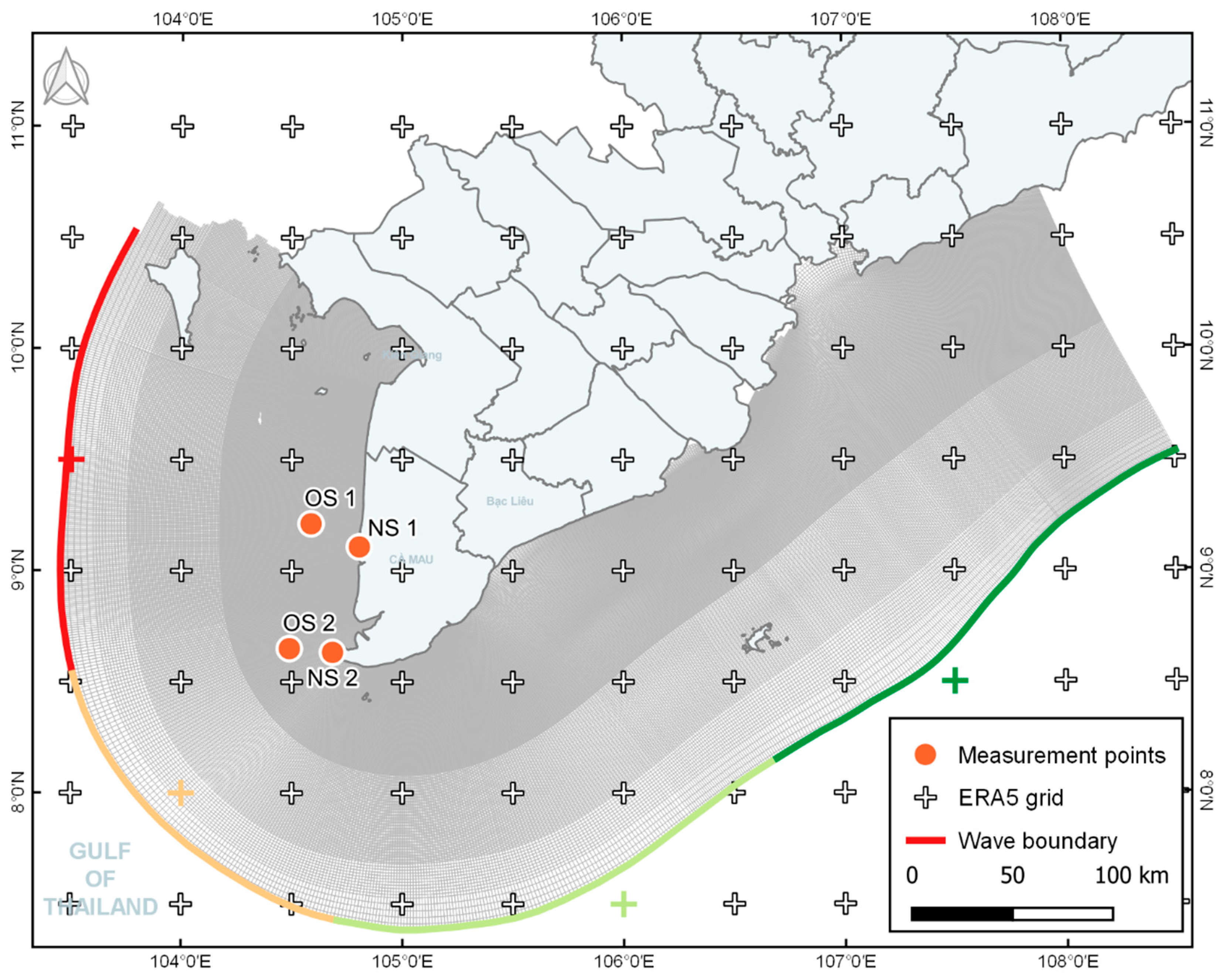
Based on the required parameters (wave height, wave period, wave direction, bathymetry) for validation of the models, the measurement campaign in July 2019 was set up to assess the wave transfer from offshore (~25 km) to nearshore along two transects at the western coast of the MD. The offshore measurement locations (OS1 and OS2), the measured bathymetry profiles, and the ERA5 grid are given in Figure 2. The offshore measurement points were thereby defined according to the ERA5 grid cells closest to the coast, comprising a resolution of 0.5° (approx. 55 km). The nearshore locations (NS1 and NS2) were chosen according to the water depth of a potential breakwater construction (1.5–2 m) with a distance to the coastline of ~500 m for the northern (Transect 1) and ~2.5 km for the southern profile (Transect 2). Each transect could be allocated to a specific ERA5 gridbox, featuring a perpendicular alignment towards the coastline. As shown in Figure 2, the position of OS1 was located approximately 11 km north to the perpendicular line of Transect 1 and NS1. Due to the parallel shape of the coastline bathymetry and the deepwater conditions at these locations, bottom friction is not relevant to the wave height. OS1 was anyhow considered as plausible input for Transect 1 in this study. While Transect 1 shows a common cross-section for the west coast with a continuously increasing bathymetry, Transect 2 at the Ca Mau cape shows a flat plain that extends approx. 15 km from the coast to the ocean followed by a sudden steep drop.

In situ data were collected from 1 July 2019 to 13 July 2019. This time was chosen to capture the peak of the southwest monsoon season in the MD. In contrast to former measurements, it was therefore intended to collect data especially from heavy sea states and over a period of several days with several sensors at the same time. Offshore and nearshore location at each transect were measured over the same period, while measurements at Transect 2 were performed after the measurements at Transect 1 due to the limited availability of sensors.

Wave and current conditions along each transect were measured over a period of at least three days by ADCP (Acoustic Doppler Current Profiler) sensors, using a Signature 1000 (Nortek, Bologna, Italy) for nearshore and AWAC (Acoustic Wave And Current Profiler) for offshore measurements applying 10 min to 15 min measurement intervals. Data extraction and processing were later performed using the SignatureWaves64 software (Nortek). To compare these measurements with the hourly available wave heights and periods from ERA5, a one-hour average was calculated over the same timesteps from the measured data and was later used for verification.

The coastal bathymetry at the western coast of the MD is very shallow and characterized by gradually increasing slopes ranging only between 1:600 up to 1:1200 for more than 10 km out to the sea (Figure 2). While the depth profile of the coastline varies along the delta, the area around the cape Ca Mau is especially flat [32]. The bathymetry along each transect was measured by echo-sounding performed during the same period. As the boat could not approach the shallow water close to the coast at Transect 2, the bathymetry for the last 3 km toward the coast could not be measured. The missing distance was completed using bathymetry data from a measurement in 2011 provided by the ICOE [33]. For comparison especially within the 2D model, the water levels were referenced to the water level measurements at Song Doc, a gauge located at the mouth of Song Doc River.

2.2. Long-Term Average and Extreme Conditions Based on ERA5 Reanalysis

For engineered breakwater dimensioning, wave heights for different return periods are needed to define the height of the structure and calculate the structural stability and the foundation based on wave forces. Within this study, a statistical analysis based on the latest fifth-generation reanalysis of the European Centre for Medium-Range Weather Forecasts, ERA5 [29], serves as input to the SwanOne model for the calculation of extreme wave heights as well as a boundary condition for the Delft3D model within the comparison approach (Section 3.2). Integrated ocean wave parameters and 10 m neutral wind speed and wind direction were downloaded from the C3S (Copernicus Climate Change Service) Climate Data Store [33] at 0.5° spatial and hourly temporal resolution. Given the large-scale circulation, the transects might have the same wave regime. When taking into account differences in bathymetry for the two transects, particularly when moving along the transect towards the coast (see Figure 2), more pronounced differences occur. In terms of different spatial resolutions of the archived meteorological and wave parameters, we used the same spatial resolution as it is important for consistency. Smaller-scale convective systems (both spatially and temporally), which caused the most pronounced peaks at Transect 1, were not fully captured by both spatial resolutions.

For the statistical description of average and extreme ocean wave conditions at the western coast of the Ca Mau peninsula, significant wave height, maximum individual wave height, peak wave period, and mean wave direction data were used for the 40-year period from 1979 to 2018. The same data for the year 2019 were used for comparison with the measurements taken during the field campaign in July 2019. In all analyses, the two ERA5 grid points centered at 9.0° N and 8.5° N at 104.5° E are used (Figure 2). These are the grid points closest to the coast, both at a distance of approximately 25 km to the western coast of the Ca Mau peninsula. ERA5 was chosen due to its high temporal resolution, which is particularly favorable for the investigation of extreme conditions, and due to its long-term availability. This decision is further justified by a previously performed comparison of ERA5 and WAVEWATCHIII hindcasts with satellite-based data, which showed an overall satisfactory performance of ERA5, while wave heights were substantially underestimated by WAVEWATCHIII over the study region [34].

For the analysis of extreme conditions, return levels for 10-, 20-, 30-, 50-, and 100-year return periods were estimated using a block maxima approach employing a Generalized Extreme Value (GEV) distribution for wind and a Gumbel distribution for significant wave height [35]. Maximum individual wave heights and peak wave periods were analyzed in the same way also using Gumbel distributions [36]. To focus on wave and wind forcing that have a direct impact on the western coast of the Ca Mau peninsula only, annual maxima, which were used as input to the estimation of return levels, were determined only for timesteps with the mean wave direction and 10 m neutral wind direction between 225° and 315°, respectively. It should be noted that this precondition excludes, for example, waves associated with Typhoon Linda in 1997 [37,38,39,40]. The parameters of the individual extreme value distributions that were fitted to the annual maxima were estimated with a Maximum Likelihood Estimator. All estimated extreme value distributions passed a Kolmogorov–Smirnov test. 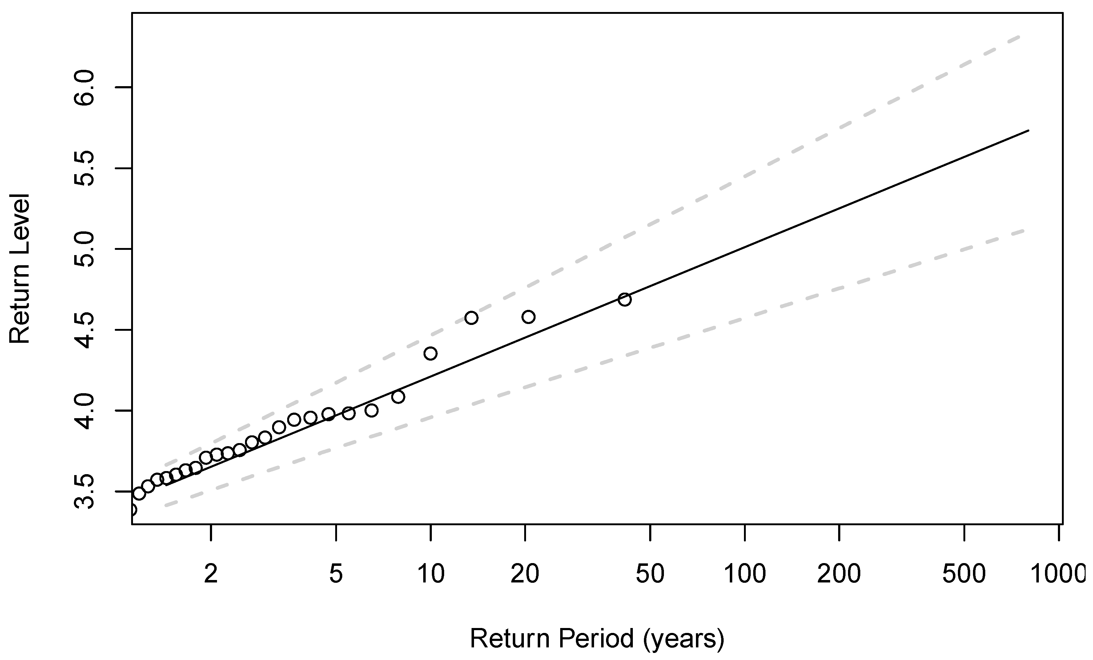Figure 3 shows the estimation of return levels of the maximum individual wave height (Hmax) at Transect 1. The results of all nine variable calculations (i.e., Hs, Hmax, Tp, and wind speed at each two transects plus the water level at Song Doc) are later provided in Table 2. Alternatively, using a Peaks-over-Threshold approach employing a Generalized Pareto distribution yields slightly lower values such that the results in

Table 1. Error and correlation analysis for the 1D and the 2D model.

Data		Benchmarks	Wave Height				Wave Period
			rho	RMSE	NRMSE	BIAS	rho	RMSE	NRMSE	BIAS
Transect 1	OS Delft3D	Input ERA5	0.80	0.05	0.11	−0.02	0.85	0.48	0.13	−0.01
		OS AWAC	0.30	0.24	0.40	−0.18	0.42	0.93	0.21	−0.65
	Input ERA5	OS AWAC	0.09	0.24	0.40	−0.16	0.45	0.77	0.17	−0.64
	NS Delft3D	NS ERA5 input	0.67	0.09	0.29	0.07	0.45	0.77	0.20	−0.58
		NS Sign measurement	0.36	0.14	0.32	−0.05	0.49	1.51	0.32	−1.38
	NS ERA5 input SWAN one	NS Sign measurement	0.08	0.16	0.43	0.12	0.27	1.03	0.22	−0.80
Transect 2	OS Delft3D	OS ERA5	0.87	0.04	0.08	0.04	0.27	0.44	0.10	0.33
		OS AWAC measurement	0.36	0.12	0.18	−0.08	−0.02	0.51	0.11	−0.15
	OS ERAS	OS AWAC measurement	0.33	0.14	0.22	−0.11	0.59	0.58	0.12	−0.48
	NS Delft3D	NS ERA5 input SWANOne	0.91	0.05	0.23	−0.04	0.36	0.39	0.19	−0.36
		NS Sign measurement	0.62	0.08	0.33	−0.07	0.31	1.37	0.53	−0.89
	NS ERAS input SWANOne	NS Sign measurement	0.76	0.04	0.19	−0.03	0.33	1.15	0.45	−0.52

can be considered as an upper bound.

Another important input parameter for both models, which is, however, not available from the ERA5 reanalysis, is the water level. For the estimation of return periods of the water level, measurements from Song Doc station were used. The longest available period of measurements from Song Doc was 1996–2015. Return levels were estimated using a Gumbel distribution and based on annual maxima during the rainy season, i.e., May to October, thus focusing on the season with predominantly southwesterly to westerly winds and waves.

In addition to the extreme values based on the statistical analysis, a historical, long-lasting extreme event was selected for a more detailed analysis. The selection of a single extreme event was based on three criteria, applied to data of the two ERA5 grid points:

• The mean wave direction is between 225° and 315°.
• The 95th percentile of significant wave height (Hs) is reached or exceeded during at least 12 h per day.
• At least three consecutive days fulfill the first two criteria.

For long-lasting events, the last criterion was relaxed to allow up to two days in-between that did not fulfill the first and/or second criterion. Based on these criteria, the eight-day period from 16th August until 23 August 2000 was selected. At the two ERA5 grid points, the maxima of Hs were reached on 22nd August (2.41 m) and 21st August 2000 (2.59 m), corresponding to approximately 32- and 28-year return periods at Transect 1 and Transect 2, respectively.

2.3. Numerical Modeling

2.3.1. Model Descriptions

In this study, SWAN was used to simulate the propagation of waves from offshore to nearshore comparing 1D and 2D model results. SWAN [41] thereby utilizes the Euler technique for time discretization to solve the spectral action balance Equation (1).

$${\displaystyle \frac{\partial }{\partial t}}N+{\displaystyle \frac{\partial }{\partial x}}{c}_{x}N+{\displaystyle \frac{\partial }{\partial y}}{c}_{y}N+{\displaystyle \frac{\partial }{\partial \sigma }}{c}_{\sigma }N+{\displaystyle \frac{\partial }{\partial \theta }}{c}_{\theta }N={\displaystyle \frac{S}{\sigma }}$$

(1)

On the left-hand side of (Equation (1)), the wave action density N(σ,θ) is used instead of energy density (N = E/σ). cx, cy are propagation velocities in geographical space, while cσ and cθ are propagations in spectral space σ and θ.

The source term on the right-hand side of (Equation (1)) according to [42] consists of the following:

S = S_in + S_wc + S_nl4 + S_bf + S_nl3 + S_br

(2)

where Sin is wind-generated waves; Swc is dissipation due to whitecapping; Snl4 is nonlinear quadruplet wave–wave interaction; Sbf is dissipation due to bottom friction; Snl3 is nonlinear triad wave–wave interaction; and Sbr is depth-induced wave breaking. While the first three sources are important in deep water, the latter three are significant in shallow water. The SWAN model represents the wave field in terms of the 2D-frequency-direction wave spectrum, which then evolves toward the coast including the effects of wind, current, water level, depth, shoaling, and refraction.

The 1D mode (SwanOne) assumes that the offshore bathymetry can be represented by parallel bottom contours such that the bottom profile can be specified along one transect that is normal to the average coastline. The 2D wave application was coupled with the numerical hydraulic module, Delft3D-FLOW. Delft3D-FLOW utilized finite-difference methods to solve the Navier–Stokes equations under the shallow-water assumption. The computational grid thereby can be rectilinear or curvilinear. Nesting techniques are available to combine different grid sizes and grid formations [43].

Each module is responsible for specific hydrodynamic processes. However, they can be coupled in integrated simulations for complex simulations when necessary. The aim was to describe the dominating main physical processes of interest, which consisted of the tidal regime, nearshore wind wave development, tidal-induced current, and wave-induced current.

2.3.2. Model Set Up and Scenario Definition

For SwanOne, the offshore-measured water levels, the wave heights, wave periods, and directions together with ERA5 wind parameters were used as input for the validation and comparison with Delft3D. Data at OS1 and OS2 were applied at the offshore boundary of the bathymetry profile. The waves were then transferred toward the coast where they were extracted again at the locations of the nearshore sensors for both transects. A sketch of the input parameters and their representation in SwanOne is given in Figure 4. All data were adapted to local time (UTC + 7 h) and were given in UTC afterwards. Wind speed and direction were taken from ERA5 for both steps due to lacking in situ data. According to the availability of ERA5 wind and wave data with a 1 h resolution, the modeling was performed for 1 h timesteps, therefore comprising only averages of the measured sub-hourly values for the wave height and wave period. For SwanOne, each timestep needed to be individually calculated with separate data input. Wave heights thereby were implemented as single wave heights. No currents were taken into account in SwanOne.

For the 2D model, the bathymetry boundary is a combination of the Gebco_2020 grid for the offshore area (GEBCO Bathymetric Compilation Group, 2020), while the nearshore zone, especially the area of interest, was supplemented with nearshore measurements from three field investigation campaigns. Two campaigns were carried out by the ICOE in 2011 [33] and 2016 [44] where the first focused on the Ca Mau cape topography, while the latter investigated the northern part of the western coast with 15 cross-profiles. In 2019, the campaign by KIT and SIWRR investigated three more cross-profiles with a length of 25 km toward the coast.

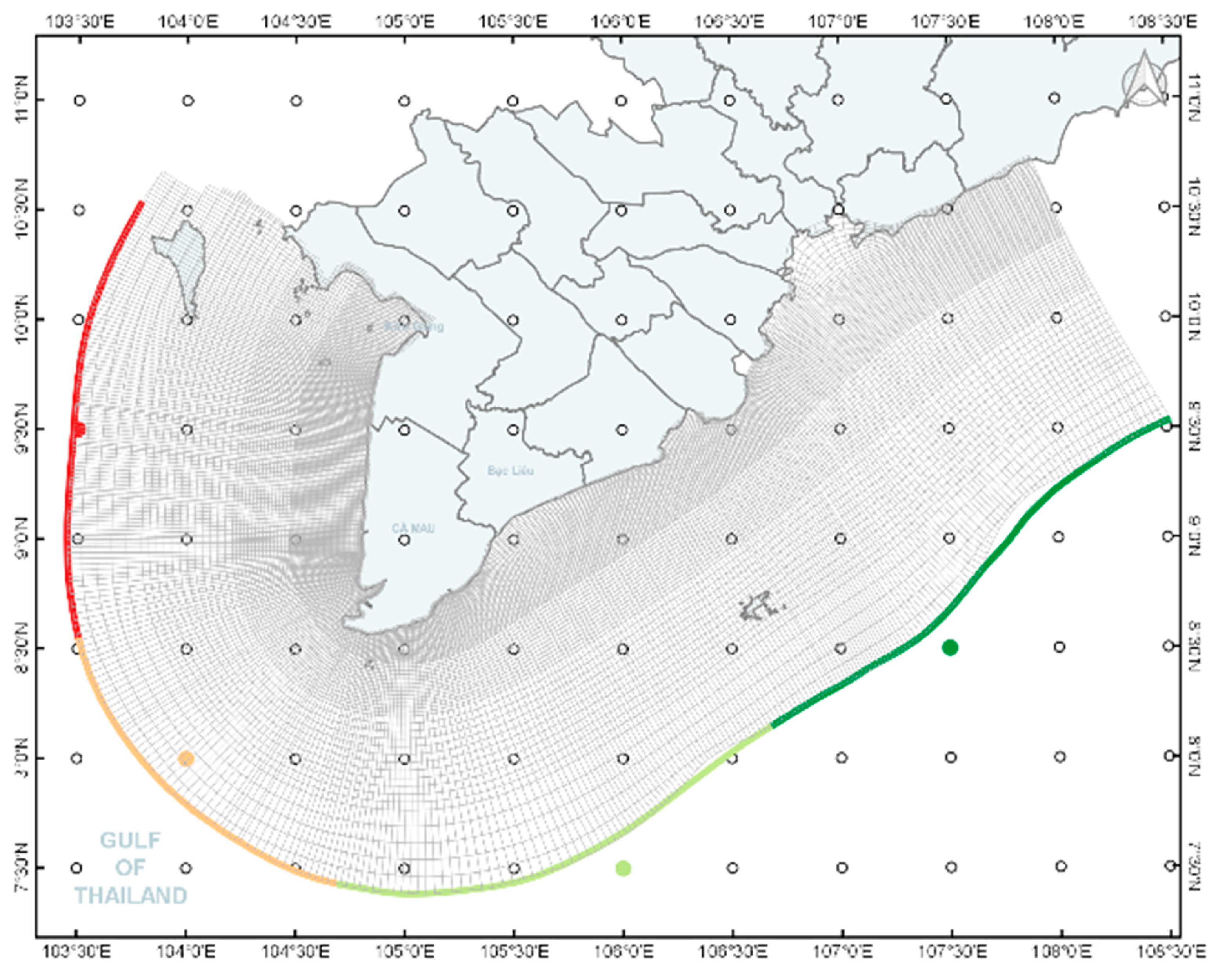
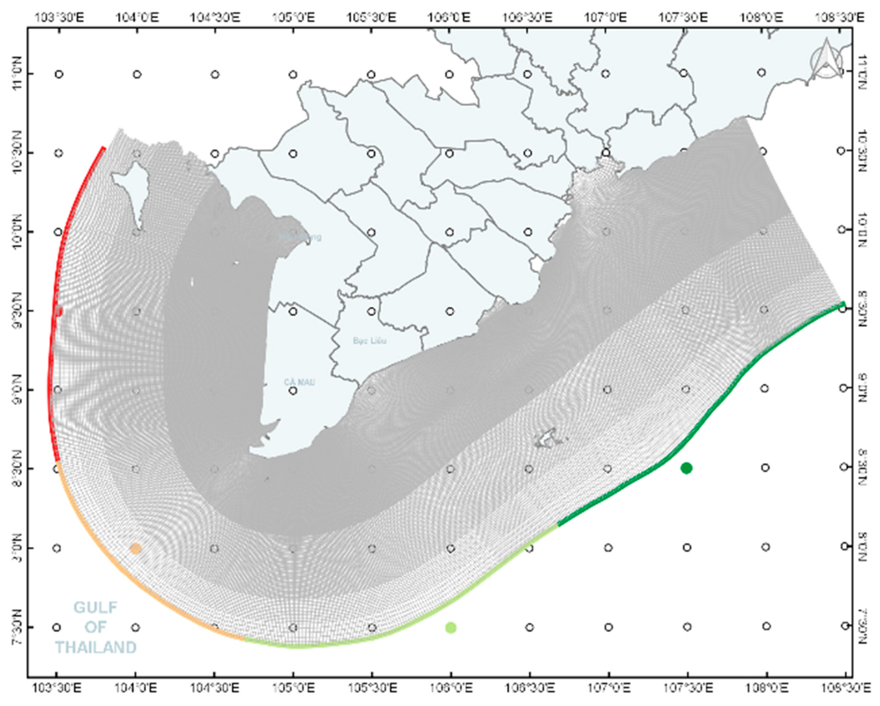
Wind force was implemented by applying hourly ERA5 data of a 10 m wind field for the whole domain [45,46]. Wave boundaries were regulated by hourly ERA5 data of wave conditions. Delft3D-WAVE was coupled with Delft3D-FLOW for fully simulating wave–current interactions within the surf zone. Tidal fluctuations were interpreted from TPXO 8.0 tidal constituents for Delft3D-FLOW [47]. A map of the final curvilinear grid, the boundaries, and the referring ERA5 wind and wave locations is given in Figure 5.

For the comparison of both models under realistic and extreme ocean wave conditions, a historical extreme event in August 2000 was selected to apply in 1D and 2D approaches. Since no long-term in situ measurements are available for the study region, ERA5 data were used for the selection of the event. The long-lasting extreme wave conditions between 16 and 23 August 2000 were related to enhanced westerly low-level winds. One factor favoring an enhanced monsoon flow was Tropical Storm Kaemi. According to the best track data of the International Best Track Archive for Climate Stewardship (IBTrACS, [48,49]), Kaemi formed on 18 August 2000 over the South China Sea and made landfall in central Vietnam on 22 August 2000. In addition, the convectively active phase of the Madden–Julian Oscillation (MJO; [50]) was located over the Maritime Continent at that time as indicated by the real-time multivariate MJO index (Wheeler and Hendon, 2004). Since the convectively active phase of the MJO can lead to enhanced westerly winds during the rainy season over Southern Vietnam [51], this might be another factor that contributed to the extreme wave conditions.

3. Results and Discussion

3.1. Model Validation

3.1.1. Swan One

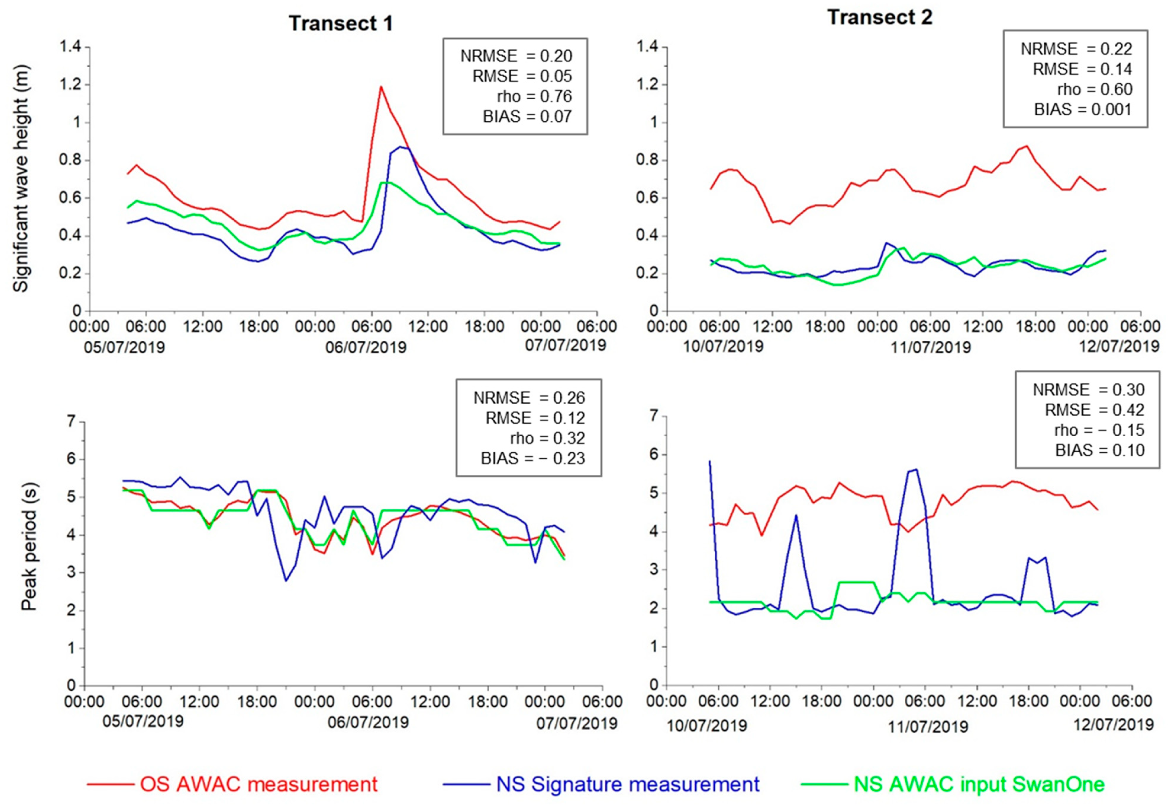
Within the verification process in SwanOne, the measured offshore wave heights (AWAC, red line) were transferred towards the nearshore and extracted again at the location of the Signature 1000 sensor (green line). Then, they were compared to the actual measured wave heights (blue line) taken from the sensor observation. The agreement of this comparison (blue line and green line) for both transects was rated satisfying, which is later shown in Section 3.1.3 for error analysis. The three pronounced peaks in the wave periods at Transect 2 originate most likely from a sensor malfunction; therefore, we excluded these unnormal data from statistical calculation in this research. By using input data with a resolution of 1 h (red), even a short-lasting storm event, which happened during the measurement at Transect 1 (start: 6 July 2019 5:00 UTC), could be reproduced successfully. The temporal shift between measured and transferred waves at the beginning of the storm might be attributed to the northern position of the AWAC sensor as described in Section 2.2. The results at Transect 1 and Transect 2 are not directly comparable due to the different measuring periods (Figure 6).

3.1.2. Delft3D

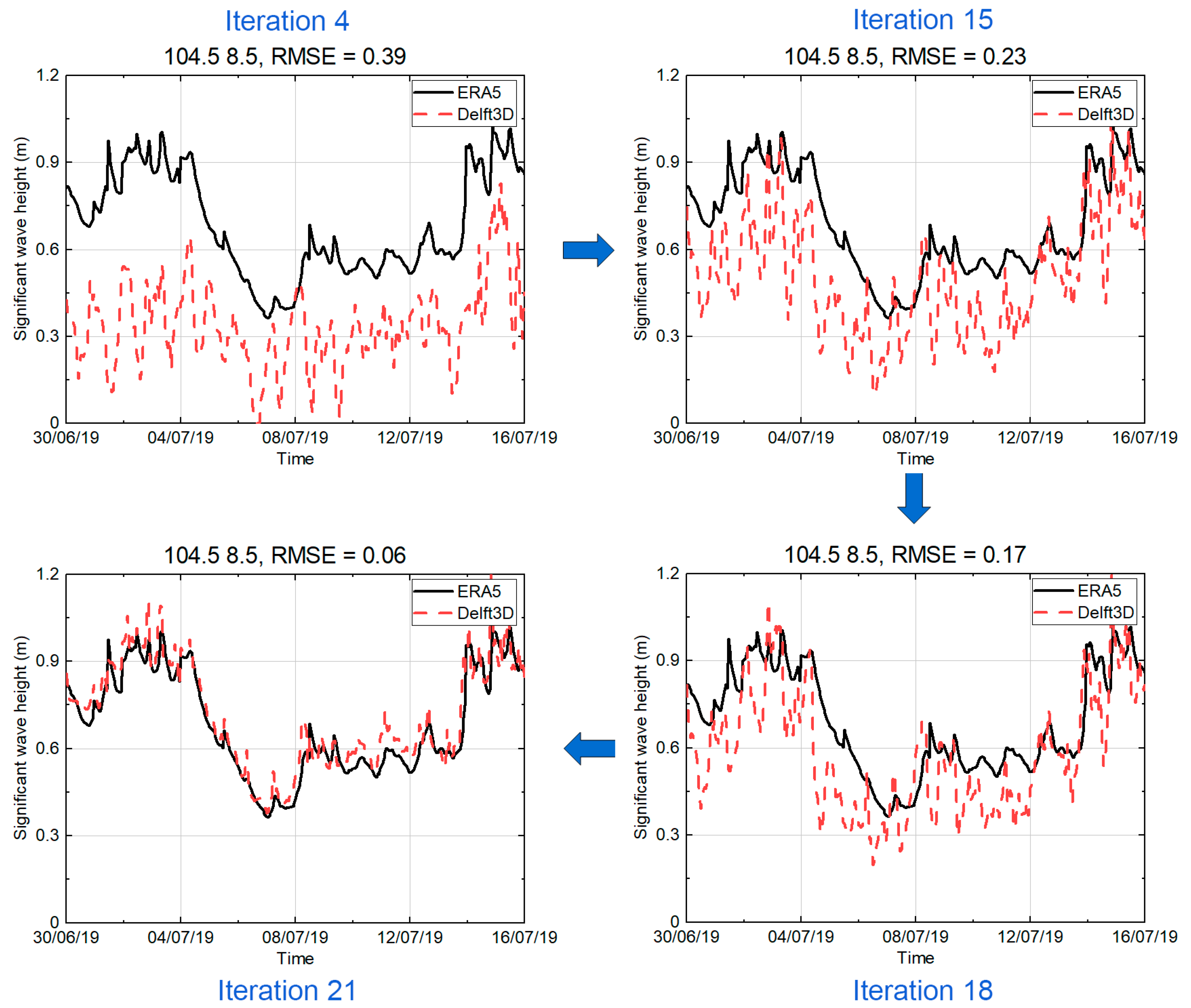
For the validation of the 2D model, a loop of adjustment was performed stepwise for the domain extent, grid type and grid resolution (see

Table A1. Iterative increase in 2D model accuracy, the list of applied grid refinement and model adaptions to the boundary conditions.

Iteration	Grid	Resolution	Extend	Adjusting
1	Regular	8 km	200 km from coast	New grid
2	Regular	8 km	200 km from coast	Adjusting grid
3	Regular	8 km	200 km from coast	Adjusting grid, improve near-shore bathymetry interpolation
4	Regular	8 km	200 km from coast	Adjusting grid, improve near-shore bathymetry interpolation
5	Regular	3 km	200 km from coast	Finer resolution
6	Regular	3 km	200 km from coast	Adjusting grid, improve near-shore bathymetry interpolation
7	Regular	3 km	200 km from coast	Adjusting grid, improve near-shore bathymetry interpolation
8	Regular	3 km	200 km from coast	Improve near-shore bathymetry interpolation
9	Regular	3 km	200 km from coast	Adjust bottom roughness
10	Regular	3 km	200 km from coast	Adjust bottom roughness
11	Curvilinear	0.8–3 km	120 km from coast	New grid
12	Curvilinear	0.8–3 km	120 km from coast	Adjusting grid, improve near-shore bathymetry interpolation
13	Curvilinear	0.8–3 km	120 km from coast	Adjusting grid, improve near-shore bathymetry interpolation
14	Curvilinear	0.2–2 km	120 km from coast	New grid, finer resolution
15	Curvilinear	0.2–2 km	120 km from coast	Adjusting grid, improve near-shore bathymetry interpolation
16	Regular	17 km	500–600 km from coast	New grid, test swell wave
17	Regular	17 km	500–600 km from coast	Adjusting grid
18	Regular	17 km	500–600 km from coast	Adjusting grid
19	Curvilinear	0.2–2 km	120 km from coast	Apply the wave boundary from ERA5
20	Curvilinear	0.2–2 km	120 km from coast	Bottom roughness, wave breaking coefficient
21	Curvilinear	0.2–2 km	120 km from coast	Bottom roughness, wave breaking coefficient

and

Table A2. Wind surge generated water depth increase at the coastline (point 113 and 118, see Figure 2) based on the Beaufort scale wind speed input to the spatial model.

Beaufort wind scale	12	11	10	9	8	7
Wind descriptive	Hurricane	Violent storm	Storm	Strong gale	Gale	Near gale
Wind speed (m/s)	>32	29–32	25–28	21–24	17–21	14–17

and Figure A1, Figure A2, Figure A3 and Figure A4 in the Appendix A), and the wave and wind boundary definition. The optimization process aims to achieve good agreement between simulation and measurement data while maintaining reasonable computational time. Along the process, it was found that grid resolution has a stronger impact on accuracy than grid type (rectangular or curvilinear). However, curvilinear, in this case, gives the flexibility to optimize the grid resolution in the nearshore area. In addition, the swell appeared to have a substantial impact on the results; therefore, applying wave conditions to the offshore boundary gives a higher efficiency in improving the swell wave prediction, in comparison to an extension of the simulation domain. Although it was recommended to use 0.019 m² s⁻³ for JONSWAP bottom friction under the condition of a smooth seafloor [52], the default value of 0.067 m² s⁻³ was selected as it showed better agreement, especially when validating with nearshore measurements. The overall process of optimizing the model accuracy along the different iteration steps is illustrated in Figure 7. The overall good agreement does not come fully unexpected due to the calibration of Delft3D against ERA5 and due to the use of 10 m neutral winds from ERA5 over the entire domain. However, since ERA5 wave spectra were only used as input at the outer boundaries of the model domain, this demonstrates that the calibration of Delft3D worked well.

3.1.3. Model Comparison

To compare SwanOne and Delft 3D over the period of in situ measurements, the same approach as in the validation was performed for SwanOne, replacing the offshore AWAC input now by the wave heights taken from ERA5.

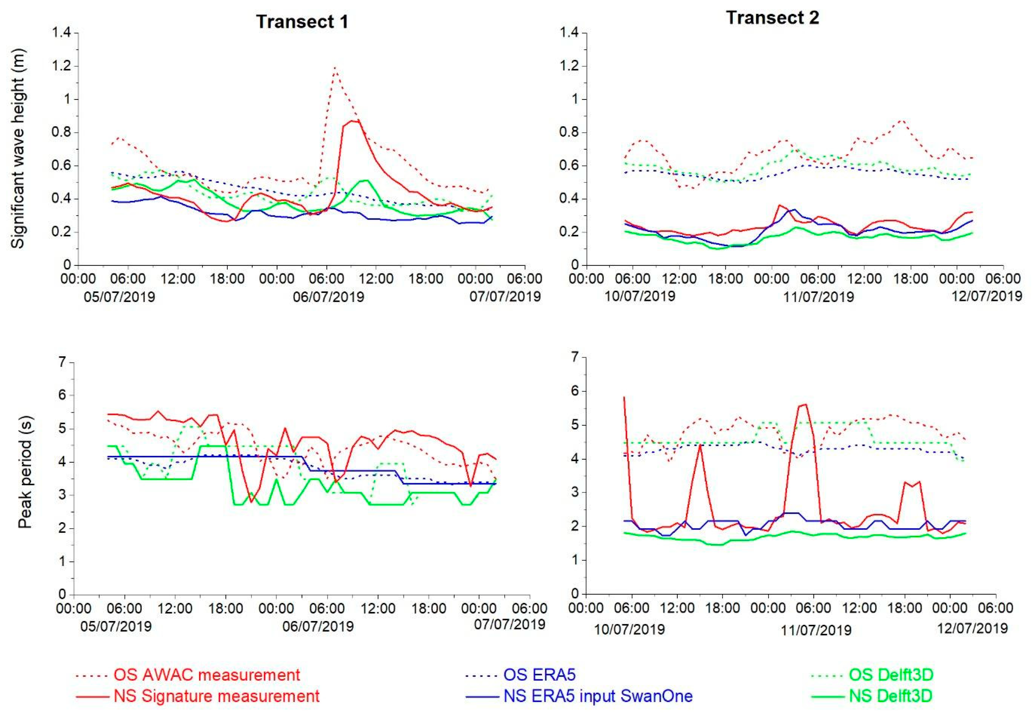
Modeling results (1D and 2D) were illustrated together with the offshore and onshore wave heights and wave periods measured during the field campaign (Figure 8). The overall range of the measured offshore wave heights and the wave heights taken from ERA5 shows a good agreement for Transect 1 until 6 July 2019 at 6:00 UTC and for Transect 2 over the entire period (10 July until 12 July). This agrees as well with the offshore conditions in the 2D model. The values for Transect 1 after this date show a strong increase in the measured wave heights due to a sudden local storm event that lasted for approx. 10 h. This short and locally confined event was not reproduced in the ERA 5 data at Transect 1 (dashed blue line) due to the coarse grid cell of ERA5 compared to the single-point measured at the sensor site. While wind speeds of ERA5 showed highest values within this period with 9.6 m/s at Transect 1, the storm did not last long enough to generate comparable wave heights by wind fetch within the 2D model (dashed green line) in comparison to the measured wave heights (dashed red line). Due to these reduced input wave heights, the nearshore output of the 2D model features this peak as well with much lower wave heights. As both models are based on the same ERA5 input regarding wave height, wave periods, wind speed and wind directions, this could be attributed to the stationary mode of the 2D model, where each timestep is influenced by the results of the timestep before, and, therefore, wind effects might constantly influence the model while the boundary wave heights remain small (dashed blue line). Due to the different measuring periods at Transect 1 and Transect 2, the storm is not included in the data of Transect 2, and the timelines of both transects cannot directly be compared to each other.

Wave periods were also compared between measured data (AWAC and Signature 1000 sensors) and the simulation results (Delft3D and SwanOne; Figure 8). At Transect 1, the wave peak periods both offshore and nearshore overall vary between 3 and 5.5 s without a pronounced reduction during the transfer from offshore to nearshore. For data featuring the same origin, like AWAC and Signature 1000 (solid and dashed red lines) or like ERA5 input and SwanOne (solid and dashed blue lines), the peak period rather remains constant from offshore to nearshore. This might be an effect of the shallow but continuously increasing bathymetry (see Figure 2), where the waves’ spectrum is not converted along its way, and, therefore, the waves are not breaking.

In contrast, Transect 2 shows a clear reduction in peak periods from offshore to nearshore for measured and modeled data. Wave periods vary from 4.0 to 5.2 s in the offshore and reduce to 1.8 to 2.2 s at the nearshore locations. This is as well an effect of the bathymetry, where the sudden seafloor increase at the edge of the shelf converts the wave towards a smaller peak period. The shallow and slowly increasing bathymetry at Transect 1 therefore might not cause enough interaction to force an incoming wave to break and change its energy spectrum. In contrast, a wave running along Transect 2 will face a strong transformation when reaching the sudden drop and therefore most likely will break and dissipate its energy. Despite the three already mentioned peaks in the wave period, the SwanOne results (blue solid line) agree well with measured data (red solid line), while the Delft3D results (solid green line) provided slightly lower wave periods (1.8 to 2 s). The difference in wave periods between measurements and numerical results is approx. 20% at both transects (ignoring the peaks) at the offshore and nearshore locations. Beside the described lack of accuracy for short extreme events, both numerical platforms showed sufficient agreement, especially at Transect 2, so the overall applicability to the further investigation was considered reliable.

3.1.4. Error Analysis

Error and correlation metrics were performed for both models for the Normalized Root Mean Square Error (NRMSE), Pearson’s correlation (rho) and BIAS (see Table 1). For wave heights and wave periods, the NRMSE ranges below 0.5, which is usually considered acceptable, while ~45% are even smaller than 0.2. Pearson’s rho shows a positive correlation for all wave heights and almost all wavelengths, mostly in the range between 0.3 and 0.9. The bias for wave heights ranges between +0.07 and −0.18. In general, Transect 2 showed a better agreement between measured and modeled values compared to Transect 1. According to this, the data for the wave height and period show sufficient agreement for both transects to accept the applicability of the 1D transfer model for further use in this study.

3.2. Applications

3.2.1. Long-Lasting Extreme Event

As for the first comparison of both models, the ocean conditions especially along Transect 2 were rather calm. They should be compared under more extreme conditions. Therefore, the 8-day lasting storm in August 2000 was selected as well for an additional comparison. According to the ERA5 reanalysis, the highest significant wave heights during the event, reaching more than 2.5 m, occurred on 22 and 21 of August at the offshore locations of Transects 1 and 2, respectively (red dashed lines in Figure 9, top left and top right).

Figure 9 shows the comparison of Hs (top) and Tp (bottom) between ERA5 and Delft3D at the offshore locations (blue and red dashed lines) and SwanOne and Delft3D at the nearshore locations (blue and red solid lines) of both transects. The output timesteps of Delft3D and ERA5 are hourly, while a 6-hourly output from SwanOne was used, which could lead to a misrepresentation of local minima or maxima. For the interpretation of the results, it should also be noted that ERA5 served as input for both SwanOne and Delft3D, due to the non-availability of in situ measurements.

The agreement between Hs from ERA5 and Delft3D is overall good at the offshore locations of both transects (Figure 9, top, dashed green and blue lines). The agreement does not depend on the wave heights, and small deviations of Delft3D with respect to ERA5 (biases not larger than ±20%, e.g., between 18th and 20th August 2000 at Transect 2) seem not to be systematic. When focusing on the nearshore locations, SwanOne and Delft3D show a good agreement at Transect 1 (Figure 9, top left). At Transect 2 (Figure 9, top right), Hs is almost constant over the entire period at the nearshore location, leading to larger differences to SwanOne, which shows more pronounced fluctuations that correspond to the ERA5 input at the offshore location. In SwanOne, higher waves and more pronounced fluctuations at the nearshore location are possible due to higher water levels. If the differences in Hs and Tp in Transect 2 were a cause of the different models used, they would also have to occur in Transect 1, which is actually not the case.

When focusing on the comparisons for wave periods (Tp), larger differences can be observed between the two Transects. At Transect 1, almost no decrease in the Tp between the offshore and nearshore location occurs (Figure 9, bottom left). At both locations, Tp varies between approximately 4 and 7 s. Overall, Tp is up to approximately 1 s shorter in Delft3D. At Transect 2, however, Tp at the nearshore location is only half of the Tp at the offshore location, decreasing from approximately 6 s to 3 s (Figure 9, bottom right). The offset of Delft3D compared to ERA5 and SwanOne is comparable to that at Transect 1. As can be seen for Hs at the nearshore location, the temporal variation in Tp at the nearshore location is relatively weak in Delft3D when compared to SwanOne. The differences in Hs as well replicate the results from the measurement campaign and are therefore most likely caused by the same bathymetry effects.

In addition to the different bathymetries used in the two modeling approaches that could lead to differences in Hs and Tp, as discussed above, there are various other potential reasons. Particularly, it is expected that Delft3D could better represent the wave conditions since it considers important factors such as wind surge, wave diffraction, wave–wave interactions, and wave–current interactions. All of these factors are not considered in SwanOne. Swell, which was found to be essential in the correct simulation with Delft3D, is considered in both models through the use of ERA5 input.

Despite the uncertainties due to the bathymetries being used in this shallow coastal area, Figure 10 illustrates the advantages of the 2D approach, where Hs and Tp at one timestep during the first period of enhanced wave heights (00:00 UTC on 17 August 2000) are shown as an example. Using Delft3D, wave conditions can easily be derived for any other location along the coast; therefore, result extraction only depends on the grid resolution of the model. Simulating ocean waves over a larger domain also allows for interaction not only with other waves, currents, and the atmosphere but also with topographic features, which manifests, e.g., in wave attenuation and diffraction at islands in the Gulf of Thailand. On the contrary, SwanOne only considers a simple, one-way interaction with the atmosphere and strongly depends on the grid spacing of the input wave conditions.

3.2.2. Calculation of Average and Extreme Conditions for Different Return Periods

After validating and comparing SwanOne and Delft3D successfully under different conditions, SwanOne was finally used for the calculation of extreme wave heights close to the coast, which are intended to be used for breakwater design. According to local dike regulations, the coastal protection for the MD needs to consider a return period of 20 to 30 years, based on the agricultural use and the population density of the protected hinterland [53]. The following step was only performed for the 1D model, as the statistical analysis of return periods from ERA5 is not possible for the 2D approach due to the lack of many boundary conditions.

Table 2. Input parameters for the 1D wave transfer model along Transect 1 and Transect 2.

Transect	Variable	Mean	Return Period [Years]
			10	20	30	50	100
Transect 1	Wind speed [m s−1]	5.80	12.88	13.38	13.68	14.07	14.62
	Hs [m]	0.68	2.19	2.32	2.40	2.49	2.62
	Hmax [m]	1.28	4.18	4.42	4.57	4.74	4.98
	Wave period [s]	4.34	7.39	7.66	7.81	8.00	8.26
Transect 2	Wind speed [m s−1]	6.02	13.28	13.80	14.10	14.47	14.98
	Hs [m]	0.75	2.36	2.51	2.61	2.72	2.87
	Hmax [m]	1.41	4.51	4.81	4.99	5.20	5.49
	Wave period [s]	4.61	7.50	7.76	7.91	8.10	8.36
All	Water level variation [cm] *	–	96.15	104.84	109.84	116.10	124.53

* water level refers to Song Doc gauge (see Figure 2).

gives the input parameters for wave heights, wave periods and wind speed, taken from the statistical analysis of ERA5 data from 1979 to 2019 for return periods between 10 and 100 years. As described in Section 2.2, only waves from a western direction were considered in this evaluation, therefore comprising mostly waves during the southwest monsoon season. The water level variations for the different return periods are based on measurements at the Song Doc hydrological station from 1996 to 2019 following the same statistical evaluation as performed for the wave heights. Due to the lack of long-term local sea level data, average water levels at Song Doc were applied for both transects following the assumption that there is not much variance of water level along the western coast. Water level variations in Table 2 therefore comprise a combination of wind surge and tides. Calculations were performed for the mean Hs and maximum Hs, whereas both refer to a respective average from the ERA5 analysis. Results for Hs are presented in Figure 8 for return periods of 10 years (green), 20 years (blue), and 50 years (red). The left column shows the decrease in wave height, while the wave is transferred from offshore (25 km) to nearshore (1 km), and the right column gives a focus on the last 1000 m towards the coast. As expected, for the intermediate and shallow water conditions, the wave height mainly follows the bathymetry profile, featuring a slight, constant decrease along the slowly rising bathymetry of Transect 1 in contrast to a sudden change at approx. 15 km distance to the coast, where the shelf plateau drops steeply for Transect 2.

As shown in Figure 11, the long-term average wave heights along the first kilometer, e.g., 100 m, range around 0.5 m corresponding to a water depth of 1.2 m at Transect 1 and approximately 0.2 m of wave height corresponding to a water depth of 1.0 m at Transect 2 (solid black lines). Maximum average wave heights at Transect 1 are around 0.7 m and are therefore substantially higher than the maximum average wave heights of 0.2 m at Transect 2 (dashed black lines).

These numbers are in good agreement with average nearshore significant wave heights from previous surveys with 0.5 m up to 0.85 m at the western coast of the MD [19]. Results at Soc Trang for wave transformation from offshore to nearshore using the XBeach model also show comparable results reducing a 2 m wave height at 10 km down to 0.5 m at the beach for comparable bathymetry conditions like at Transect 1.

Related to the coastal protection, e.g., by detached breakwaters, wave heights for return periods of 20 years at a realistic implementation distance between 100 m up to 300 m to the coast range from 1.1 m to 1.3 m corresponding to water depths of 2.33 m to 2.88 m at Transect 1, while wave heights at Transect 2 range approximately 0.65 m corresponding to a water depth of 2.12 m. Maximum wave heights for the same return period and distance show negligibly higher values for both transects. This might be attributed to the fact that the wave heights in shallow water near to the coast are already close to the physical limit.

As a well-known fact, wave heights are significantly dependent on water depth, especially for the shallow nearshore zone. Increasing water levels, therefore, would directly increase the maximum possible wave height at the coast. Under extreme weather conditions, water levels could also rise due to stable wind stress (wind surge). This phenomenon was demonstrated using Delft3D by coupling the two modules Wave and Flow and applying winds with constant high speeds and directions to the model over an extended period of time. Within this test, the water depths are increased for approx. 1 m at a constant wind scale of 9 while they are up to 2 m at a wind scale of 11, therefore demonstrating a kind of worst-case wind swell scenario (see SM6 and Figure 10). However, it must be emphasized that increasing water depths would increase the submergence of any breakwater accompanied by wave overtopping rates. Therefore, extreme surge conditions would not inevitably lead to an adaptation of the breakwater design regarding its stability. Unfortunately, under such conditions, the waves can again hit the coastline without any prior reduction.

3.3. Limitations of This Study

According to the different input sources, wave heights were available as Hs (calculation based on measured wave heights) and Hm0 (statistical analysis based on energy spectrum) from the sensors, while ERA5 only features Hm0. To remain consistent, all calculations were performed based on Hm0. As a comparison of Hs and Hm0, the measurements showed slightly higher values for Hm0 (around 5%). These overall results within this study might overestimate the significant wave height.

While the AWAC at Transect 1 showed reasonable data regarding the wave directions, the wave directions at Transect 2 were rather inconsistent. During the launching of the wave sensor in the field, the AWAC sensor at Transect 2 was tilted by around 12°, which is slightly above the suggested operation range (10° according to Nortek). Nevertheless, it was still below the acceptable limit of 20°. Therefore, tilt effects were removed during the post-processing of the data. In addition, some of the measured wave frequencies were close to the range that the sensors cut off, which might be an additional source for inaccuracies. The wind direction from ERA5 was taken as input for the wave direction instead at Transect 2 as both typically coincide if the wind comes from a constant direction over longer periods.

As the measured data at Transect 2 were rather inconsistent, the results at this transect should be treated with caution. However, due to the fact of high agreement between the 1D and 2D numerical approaches, the selection of alternative boundary conditions in the case of inadequate sensor measurements seems sufficient. We decided to present these results in this study, as the availability of data and related studies is scarce in this area. In addition, Transect 2 for practical reasons is of minor relevance, as it is located at the tip of the Ca Mau peninsula, an area of natural soil deposition processes, with no actual needs for coastal protection.

Concerning the models, bottom friction could not be included for SwanOne based on the restriction of the software. The input of currents would have been possible; however, the single-point current measurements showed unrealistic values compared to the local conditions and were therefore not considered for further processing. Current profiles were also not explored with Delft3D. Our nearshore sensor was struggling with reasonable current data, which we suspect were due to a very low water depth at the location of deployment. In addition to that, our study is focusing on wave transferring from offshore to nearshore, while the current might have a significant impact on wave conditions nearshore as long as the incoming wave direction and current direction are parallel to each other, e.g., near outlets or river mouths. This fortunately was not the case of our location of interest. The tidal current mainly follows the coast line (North—South and vice versa). Good validation results with measured wave conditions also support this assumption of current impact as it is minimal for this study.

4. Conclusions

In this study, a stepwise approach to the determination of dimensioning conditions for breakwater design is presented based on a combination of measurements, long-term reanalysis data, and numerical approaches.

In the first step, ERA5 offshore data could be successfully downscaled to two onshore locations with SwanOne and Delft3D and validated by observations. As a second, during a storm event of several days in 2000, both numerical platforms were used to compare the applicability of the wave transfer approach based on ERA5 reanalysis data as input in the Gulf of Thailand. Both steps thereby showed consistent results.

Finally, SwanOne was used to calculate nearshore wave heights and periods for mean, 10-, 20-, 50- and 100-year return periods at the western coast of the MD, which derived from a 40-year ERA5 time series analysis. Breakwater design for a 20-year return period in a realistic implementation distance between 100 m up to 300 m to the coast thereby ranges from 1.1 m to 1.3 m at Transect 1 and 0.65 m at Transect 2. This is corresponding to water depths of 2.33 m (100 m) and 2.88 m (300 m) at Transect 1 and 2.12 m at Transect 2. The average wave heights therefore are in good accordance to previously published data.

In comparison of the models, both numerical approaches showed a sufficient agreement with the observations and therefore are both applicable for the reason of dynamic downscaling of climate reanalysis data. Both numerical approaches showed their capabilities. SwanOne offers a simple and fast calculation method, while it lacks in continuous effects like wind-generated swell or bottom friction. The Delft3D software, on the other hand, provides a more complete representation, not only of wave but also current dynamics, while it requires a much broader amount of input parameters and more complex boundary conditions. One major advantage of SwanOne, thereby, is its applicability to wave conditions derived from statistical extreme value analysis, which cannot easily be prepared in a similar way for Delft3D.

The shortcomings within this study are directly connected to the available temporal resolution of the ERA5 data and its rather coarse grid size as both models underestimate the extreme conditions compared to the measured values as a result of an insufficient representation of the storm by ERA5 due to the spatio-temporal resolution. In addition, as the overall data availability in this area is still insufficient, the set up of long-term measurement stations for wind and waves is highly recommended, especially against the background of the problems connected to coastal erosion and climate change as mentioned in the introduction. Here, it would be valuable to supplement the existing study as well for different climate change scenarios.

According to the scarce availability of nearshore long-term observations in the Gulf of Thailand, this study might serve as a template for further projects to derive nearshore wave conditions by means of targeted short-term measurements and climate analysis.