Article

Band Weight-Optimized BiGRU Model for Large-Area Bathymetry Inversion Using Satellite Images

Key Laboratory of Spatial-Temporal Big Data Analysis and Application of Natural Resources in Megacities (Ministry of Natural Resources), Shanghai Municipal Institute of Surveying and Mapping, No. 419 Wuning Road, Shanghai 200063, China
*
Author to whom correspondence should be addressed.
J. Mar. Sci. Eng. 2025, 13(2), 246; https://doi.org/10.3390/jmse13020246
Submission received: 6 January 2025 / Revised: 22 January 2025 / Accepted: 24 January 2025 / Published: 27 January 2025
(This article belongs to the Special Issue New Advances in Marine Remote Sensing Applications)

Abstract

:
Currently, using satellite images combined with deep learning models has become an efficient approach for bathymetry inversion. However, only limited bands are usually used for bathymetry inversion in most methods, and they rarely applied for large-area bathymetry inversion (it is important for methods to be used in operational environments). Aiming to utilize all band information of satellite optical image data, this paper first proposes the Band Weight-Optimized Bidirectional Gated Recurrent Unit (BWO_BiGRU) model for bathymetry inversion. To further improve the accuracy, the Stumpf model is incorporated into the BWO_BiGRU model to form another new model—Band Weight-Optimized and Stumpf’s Bidirectional Gated Recurrent Unit (BWOS_BiGRU). In addition, using RANSAC to accurately extract in situ water depth points from the ICESat-2 dataset can accelerate computation speed and improve convergence efficiency compared to DBSCAN. This study was conducted in the eastern bay of Shark Bay, Australia, covering an extensive shallow-water area of 1725 km2. A series of experiments were performed using Stumpf, Band-Optimized Bidirectional LSTM (BoBiLSTM), BWO_BiGRU, and BWOS_BiGRU models to infer bathymetry from EnMAP, Sentinel-2, and Landsat 9 satellite images. The results show that when using EnMAP hyperspectral images, the bathymetry inversion of BWO_BiGRU and BWOS_BiGRU models outperform Stumpf and BoBiLSTM models, with RMSEs of 0.64 m and 0.63 m, respectively. Additionally, the BWOS_BiGRU model is particularly effective in nearshore water areas (depth between 0 and 5 m) of multispectral images. In general, comparing to multispectral satellite images, using the proposed BWO_BiGRU model to infer hyperspectral satellite images can achieve better bathymetry inversion results for large-area bathymetry maps.

1. Introduction

Shallow water bathymetry has attracted much attention in recent years. It has a significant influence on coastal topography and landform mapping, coral reef habitat mapping, coastal zone and seabed environment construction, marine geological disaster prediction, and benthic organism protection [1,2,3,4,5,6,7]. Currently, common methods for measuring shallow water depth include ocean sonar technology, physical methods, stereo photogrammetry [8,9,10], active Light Detection and Ranging (LiDAR), passive optical remote sensing technologies, and other traditional models. Marine sonar technologies include single-beam echo sounding (SBES) [11], multi-beam echo sounding (MBES) [12], and sidescan sonar sounding (SSS) [13], which can collect high-resolution bathymetry data but also have shortcomings such as high cost and limitations due to weather and geographical environments. Physical methods include wave kinematics [14,15,16,17] and gravity geological methods [18,19,20], which can all describe underwater terrain but are limited by differences in various geophysical characteristics. LiDAR [21,22,23] and Synthetic Aperture Radar (SAR) [24,25] have also received more attention particularly. ICESat-2, which was launched in 2018 and carries the Advanced Terrain Laser Altimeter System (ATLAS) [26], has been used widely for many land and water-related applications. These methods can measure high-resolution water depth data, but due to the influence of meteorological conditions, the bathymetry measurement effect is not good in cloudy and rainy weather. Satellite-Derived Bathymetry (SDB) is the calculation of shallow water depth from active or passive satellite sensors. Optical imaging technology is mainly used in SDB for bathymetry inversion from multispectral satellites (Landsat series [27,28,29], Sentinel-2 [30,31,32], etc.) or hyperspectral satellites (Hyperion [33,34,35], PRISMA [36,37,38,39], and EnMAP [40,41,42], etc.). Satellite images can cover a wide range of shallow-water areas, have low acquisition costs, and have been widely used in water depth measurement. Traditional models include the Lyzenga model [43], the Stumpf model [44], and other statistical models [45], etc. These methods are easy to be applied because they only use the red, green, and blue bands of images or their combined (additive or ratio) bands. The disadvantage is that only very few bands are used in those models; therefore, the information of all bands cannot be fully used, especially when more bands are available.
Currently, deep learning models are more and more used in shallow water bathymetry, usually outperform physics-based methods [46,47], and can provide excellent bathymetry predictions [48]. Compared to a support vector machine (SVM) [49], a deep convolutional network (DCN) [50] through nonlinear transformation can further improve the accuracy of bathymetry measurement. The enhanced SR-ResNet model fully utilizes the information of image data to generate high-resolution bathymetry data [51]. Reliable and accurate bathymetry estimates can be obtained using deep convolutional neural networks (CNNs) and unmanned surface vehicles (USVs) [52]. The BathyNet model combines photogrammetry and radiometry methods to predict water depth from multispectral aerial imagery [53]. The DL-NB deep learning framework uses in situ water depth points measured by ICESat-2 and Sentinel-2 images to perform nearshore bathymetry better than machine learning methods [54]. The FWConv method processes point cloud data from airborne LiDAR and can achieve a seabed elevation accuracy of 0.20 m [55]. In summary, the combination of deep learning models and existing methods can achieve efficient bathymetry measurement and make up for the shortcomings of a single bathymetry measurement technology. On the other hand, deep learning models are more complex. If satellite images are used to draw bathymetry inversion maps over a large area, also it needs to be considered that the inversion model should be more lightweight and automated so that it can be easily promoted in other bathymetry areas.
In the previous work, the authors have proposed the Band-Optimized Bidirectional LSTM (BoBiLSTM) model [56] and Attention-based Band Optimization CNN (ABO-CNN) model [57] to improve the accuracy of bathymetry inversion through band screening and band optimization. However, for large-area bathymetry inversion from satellite images, the band screening work of the BoBiLSTM model is particularly complicated. It is necessary to observe the missing bands of multiple images in order to determine which important bands to select. The bathymetry prediction accuracy of the ABO-CNN model in multispectral images is slightly lower, and the estimated water depth is prone to be slightly deeper in extremely shallow-water areas. In response to the above problems, a new model—Band Weight-Optimized Bidirectional Gated Recurrent Unit (BWO_BiGRU)—is proposed based on the characteristics of hyperspectral satellite images with a large number of bands and narrow spectral range. By adding the characteristic information of the Stumpf model, the Band Weight-Optimized and Stumpf’s Bidirectional Gated Recurrent Unit (BWOS_BiGRU) model is also proposed for less bands and wider spectrum ranges of multispectral satellite images. The BWO_BiGRU model uses two algorithms, namely a self-attention mechanism and a two-layer bidirectional GRU model. The self-attention mechanism is a special attention mechanism that can focus on the correlation between the satellite image’s neighboring pixels and assign different weight information to different bands by establishing a connection with water depth data. The logic unit of the BiGRU model reduces a gate control structure and is more lightweight than the BiLSTM model. Therefore, the model takes less time during the training process and is easier to converge, making it suitable for mapping large-area bathymetry. The BWOS_BiGRU model uses the above two methods and adds the band ratio of the Stumpf model in the input stage as an extra important feature that affects bathymetry inversion. This method can further enhance the bathymetry inversion of shallow-water areas for multispectral image data. The study site selected for the experiment is the eastern bay of Shark Bay, Western Australia. The research contributions of this paper are as follows: (1) Two bathymetry inversion models, BWO_BiGRU and BWOS_BiGRU, were proposed for hyperspectral and multispectral satellite images, respectively. Both models yielded bathymetry maps superior to the traditional Stumpf model. (2) It is proved that using the RANSAC method to extract ICESat-2 depth points is an efficient way for mapping large-area bathymetry from satellite images.

2. Materials and Methods

2.1. Analysis Area

Shark Bay in Australia consists of two elongated bays, the chosen part of which is the eastern bay, about 85 km (north–south) and 30 km (east–west). It covers an area of approximately 1725 km2, with geographical coordinates ranging from 113°56′ E to 114°14′ E (longitude), and 25°40′ S to 26°30′ S (latitude). The clear water quality of this area is listed on the World Heritage List and has the largest seagrass habitat environment in the world [58]. Therefore, it is the most ideal area for bathymetry inversion. Figure 1a shows the study area, using the RGB base map generated by EnMAP images. The displayed RGB channels are bands 45, 21, and 12 of EnMAP (see Table 1), respectively. In Figure 1a, line segments AB, CD, and EF represent the trajectories of ICESat-2 on 20210626GT1R, 20201215GT3L, and 20220613GT1R, respectively. These trajectories are utilized for method comparison and result analysis in the subsequent sections of the paper. In Figure 1b, solid lines of different colors represent different trajectories of ATLAS laser scanning, with 18 ICESat-2 strip data information on the right side. Figure 1c shows the location of Shark Bay in Western Australia.

2.2. Datasets

2.2.1. EnMAP–Hyperspectral Satellite Images

The EnMAP satellite was developed by the German Alliance of Earth Observation Agencies and successfully launched on 1 April 2022. EnMAP is equipped with a pushbroom prism-based dual spectrometer instrument that can acquire 224 bands, covering the spectrum range of 420–2450 nm. There are 91 VNIR bands with a spectrum range of 420–1000 nm, and a total of 133 SWIR bands with a spectrum range of 900–2450 nm. According to previous research [56], the spectral range of hyperspectral satellite bathymetry inversion is mainly concentrated in the coastal blue, visible light, and near-infrared bands, so the first 67 bands were selected from the VNIR band. The experiment used 3 EnMAP images with product type L2A, employing a Combined Correction Type and a spatial resolution of 30 m. The selected images for the study area were all cloud-free, with the water bodies appearing very clear. Three scenes were acquired from 3:09:20 to 3:09:24 on 2 May 2023 (UTC). The three scenes were mosaicked to form a large image for processing convenience sake. The band names and spectrum ranges of EnMAP are shown in Table 1.

2.2.2. Sentinel-2–Multispectral Satellite Images

The Sentinel-2 satellite was a high spatial resolution multispectral imaging satellite launched by the European Space Agency on 23 June 2015. The multispectral imager (MSI) carried by the satellite has ground resolutions of 10 m, 20 m, and 60 m and can obtain information in 13 wavebands including coastal aerosol, visible light, near infrared, and shortwave infrared. The spectrum range involved is 433–2280 nm. The experiment used three Sentinel-2 image tiles, all acquired over a cloud-free study area. The product type for all image tiles was L2A, and the acquisition time was 2:32:51 on 16 October 2023 (UTC). SNAP software (The version is 9.0.0) was used to convert the bands of Sentinel-2 satellite image tiles into ENVI format, and the spatial resolution was resampled to 30 m. The band name and spectrum range of Sentinel-2 are shown in Table 1.

2.2.3. Landsat 9–Multispectral Satellite Images

The Landsat 9 satellite was jointly developed by NASA and USGS and successfully launched on 27 September 2021. The satellite is equipped with Land Imager 2 (OLI-2) and Thermal Infrared Sensor 2 (TIRS-2), which can obtain information in 11 bands. The spectrum range involved is 433–2294 nm, with the spatial resolution of bands 1 to 7 and 9 being 30 m, the spatial resolution of band 8 being 15 m, and the spatial resolution of bands 10 and 11 being 100 m. The experiment used a Landsat 9 satellite image of a cloud-free study area. The image had a product type of Collection 2 Level 2, was acquired at 2:22:34 on 31 October 2023 (UTC), and included bands 1–7 and band 10, which were chosen for further processing. The band names and spectrum ranges of Landsat 9 are shown in Table 1.

2.2.4. ICESat-2 ATL03 Data

ICESat-2 is the second-generation spaceborne LiDAR satellite launched by NASA on 15 September 2018. The main purpose of the satellite is to monitor changes in elevation information such as polar glaciers, seawater, and forest vegetation, which is of great significance for the quantitative assessment of global ecological balance. ICESat-2 uses photon counting LiDAR (ATLAS) and positioning assistance systems to capture information such as the time, longitude, and latitude of photons reflected after being emitted to the earth’s surface. The laser pulses emitted by ATLAS can form three pairs of ground trajectories, each pair containing a strong photon trajectory and a weak photon trajectory, with an energy ratio of approximately 4:1. The experiment used the ATL03 product of ICESat-2, which includes the elevation information and geodetic latitude and longitude information of each photon. The geographical coordinate reference used is the WGS84 ellipsoid. This study selected 6 ATL03 datasets, including 17 photon trajectories (shown as solid lines of different colors in Figure 1b). The specific attributes are shown in Table 2.
Previous studies [59,60] used DBSCAN to cluster and hierarchize photons on the water surface and underwater bottom. If the study area is small, this method is a simple and effective density clustering method. However, the research area is about 1700 km2, and the 17 photon trajectories involved include noise data and valid data, with a data volume of up to millions. If this method is applied with limited hardware resources, it would require a substantial amount of time. Additionally, if the study area is in extremely shallow waters with poor water quality, it becomes challenging for this method to distinguish between photons from the water surface and those from the seafloor. Therefore, it is evidently time consuming and labor intensive to use this method for mapping in situ water depth points over a large area. The ground trajectory formed by the ATLAS laser pulse actually forms a section perpendicular to the ground. On the tangential surface, the sea level is a straight line, the seabed is a polyline, and other points are noise data. Therefore, this study considers reducing the dimensionality of photon data in three-dimensional space to lines on a two-dimensional plane. Water depth data processing, as shown in Figure 2, includes the following steps: (1) Use the RANSAC [61,62] method to cluster ATL03 data and fit them into a straight line model, and then extract the sea surface straight lines and seabed polylines, respectively. Other scattered points are noise data and are directly removed. (2) Use the elevation difference between the seafloor polyline and the sea surface straight line to obtain uncorrected bathymetry data. (3) Calculate the bathymetry data corrected by seawater refraction based on the laser pulse incident angle (ref_elev) of different photon trajectories and the refractive index of seawater (1.34116). (4) Consult the tide table of the study area [63] to calculate the tide-corrected bathymetry data. This method is suitable for ATL03 data processing of large areas of water. When the data volume of effective laser points is large enough, even a slight loss of bathymetry points on the section can be ignored.
In Figure 3, the green and red lines represent the bathymetry data extracted after preprocessing the 20201215GT3L data (yellow line segment CD in Figure 1a) of ICESat-2 using DBSCAN and RANSAC methods, respectively. The DBSCAN method (green line) clustered approximately 11,000 bathymetry points, displaying a serrated pattern. The RANSAC method (red line) clustered around 15,000 bathymetry points, showing a piecewise linear effect. Furthermore, the bathymetry trend of the red line is consistent with that of the green line. In Figure 3, the green ramp lines indicate a failure of DBSCAN clustering, resulting in missing bathymetry data. In this region, the bathymetry data clustered by RANSAC method exhibit a relatively large oscillation amplitude. This indicates the presence of turbid water conditions in the current water area. The DBSCAN method struggles to distinguish between the water surface and seafloor, while the RANSAC method, with its line fitting clustering, can effectively extract bathymetry data.

2.3. Methods

2.3.1. Stumpf

Based on multispectral satellite images, hyperspectral satellite images, and ICESat-2′s bathymetry points, this study uses two existing methods to train the model for bathymetry inversion. The first method uses the Stumpf model [44], which is currently the most classic model for remote sensing optical bathymetry inversion. This model establishes a linear model based on the logarithmic ratio of the water body’s absorption rate of energy in different wavebands to changes in water depth, making it capable of estimating water depth in shallow waters.

2.3.2. BoBiLSTM

The second method uses the BoBiLSTM deep learning model [56], which uses the Band Optimization Method to screen out the bands and band ratios related to bathymetry inversion. The algorithms involved include the Stumpf model and GBDT method. The Stumpf model selects two bands and a band ratio related to bathymetry inversion. The GBDT method selects the band with an important feature proportion and reaching 90% from all bands, as well as the important blue–green band ratio. After screening, several important bands and two band ratios are retained to participate in the training of the BiLSTM model. This method is relatively complex, but by deleting bands that contribute little to bathymetry inversion, the model can enhance the characteristics of other bands and band ratios and achieve good bathymetry inversion results when the training data are small and evenly distributed.

2.3.3. BWO_BiGRU Model

The BWO_BiGRU model uses a self-attention mechanism to assign weights to different spectral bands in a large and complex input dataset, emphasizing bands that have the most significant impact on the current output while assigning lower weights to bands that are less important for bathymetry. These weighted bands are involved in training the BiGRU model, enabling the deep learning model to achieve the capability of large-area bathymetry inversion. This method is a bathymetry inversion method that improves efficiency. It does not require additional work of filtering bands and focuses attention directly on the band information with important characteristics, thereby reducing the calculation time of noisy data.
  • Self-attention mechanism
The self-attention mechanism, also known as intra-attention [64], is an attention mechanism that focuses on the relationship between input sequence elements. The self-attention mechanism is a special attention mechanism that is good at capturing the correlation within the input data.
For hyperspectral satellite images, the feature importance of the bands in each pixel will also be dispersed as the number of bands increases, and the number of bands related to water depth inversion is concentrated in certain spectral ranges [56]. If a large-area bathymetry inversion map is to be drawn, the correlation between adjacent bands in adjacent pixels of satellite images becomes critical. For example, if the band information of a certain pixel is missing, but the adjacent band information is not missing, then they will have a certain correlation in the bathymetry inversion. According to this idea, the self-attention method is used; that is, the band information input by each pixel is associated with other band information, and the long dependence between bands in hyperspectral satellite images is captured by calculating the relative importance between bands.
  • BiGRU (Bidirectional Gated Recurrent Unit)
The Gated Recurrent Unit (GRU) [65,66] is a variant of the LSTM [67] and is a special gated recurrent neural network. The LSTM has three gate control structures, namely input gate, output gate, and forget gate, while the GRU can regulate the transmission of information flow through two gating structures: update gate and reset gate. At the same time, the GRU does not have a storage unit for storing long-term memory. Therefore, the GRU has fewer parameters than the LSTM and has lower computational complexity. The model converges more easily during the training process and improves efficiency. Considering the use of satellite images to draw large-area bathymetry inversion maps and enhancing bidirectional learning of water depth in shallow and deep-water areas, this paper proposes using the Bidirectional GRU method (BiGRU) as the basic algorithm for the bathymetry inversion model.
  • Band Weight-Optimized Algorithm
The spectral range associated with the inversion of water depth form satellite imagery includes coastal blue, blue, green, red, and near-infrared bands. The weight information affecting water depth variations varies significantly in different water bodies or different satellite images. For multispectral images, the green band has only one spectral band, and it carries only one piece of information regarding water depth. In contrast, in hyperspectral images, the impact on water depth is concentrated in several green bands, each with different weight information. In such a scenario, assigning different weights to spectral bands can enhance the sensitivity of different bands in bathymetry inversion, thereby improving the accuracy of bathymetry estimation. On the other hand, if certain pixels in satellite images experience band loss, neighboring bands with different weights can compensate for some information, preventing the loss of bathymetry inversion results. Therefore, based on these considerations, this paper proposes a band weight-optimized algorithm.
The band weight-optimized algorithm (shown in Figure 4) is a new algorithm composed of self-attention and two layers of GRUs with opposite directions.
In the band weight-optimized algorithm, the self-attention mechanism filters out a large amount of input band information to identify bands that are important for bathymetry inversion changes, gives different weights to the different bands, and finally transmits the bands to BiGRU. As a deep learning model, BiGRU can further optimize all bands with weight information to obtain more important band features, while bidirectional learning can add more features in shallow and deep-water areas. In this way, the correlation between all band data and water depth can be estimated.
For hyperspectral satellite imagery, the spectrum is narrow and dense, with different bands carrying a substantial amount of valuable information. In contrast, multispectral satellite imagery has a wider and sparser spectral range, with the effective information concentrated mainly in the blue and green bands. As a result, feature learning for shallow and deep-water areas might not be sensitive, leading to synchronous predictions of deeper or shallower water depths in bathymetry inversion. Therefore, this study introduces a band weight-optimized and Stumpf’s bidirectional gated recurrent unit (BWOS_BiGRU) method. In the input stage, the model not only includes all bands but also adds the logarithmic ratio of bands using the Stumpf model as a significant additional feature. The Stumpf model reveals that the Digital Number (DN) values in shallow-water areas exhibit higher sensitivity to logarithmic transformations, while the DN values in deep-water areas experience smaller changes after logarithmic transformations. This ensures that the BWOS_BiGRU model exhibits robustness in bathymetry inversion from multispectral satellite imagery. Whether it is hyperspectral or multispectral imagery, the band weight-optimized algorithm captures the distinctive features of each band without omission. This is of significant importance for mapping water depth from satellite imagery on a large area. In the training phase, this algorithm incorporates the geographic coordinates of in situ bathymetry points as a sequence, contributing to the bathymetry inversion process.
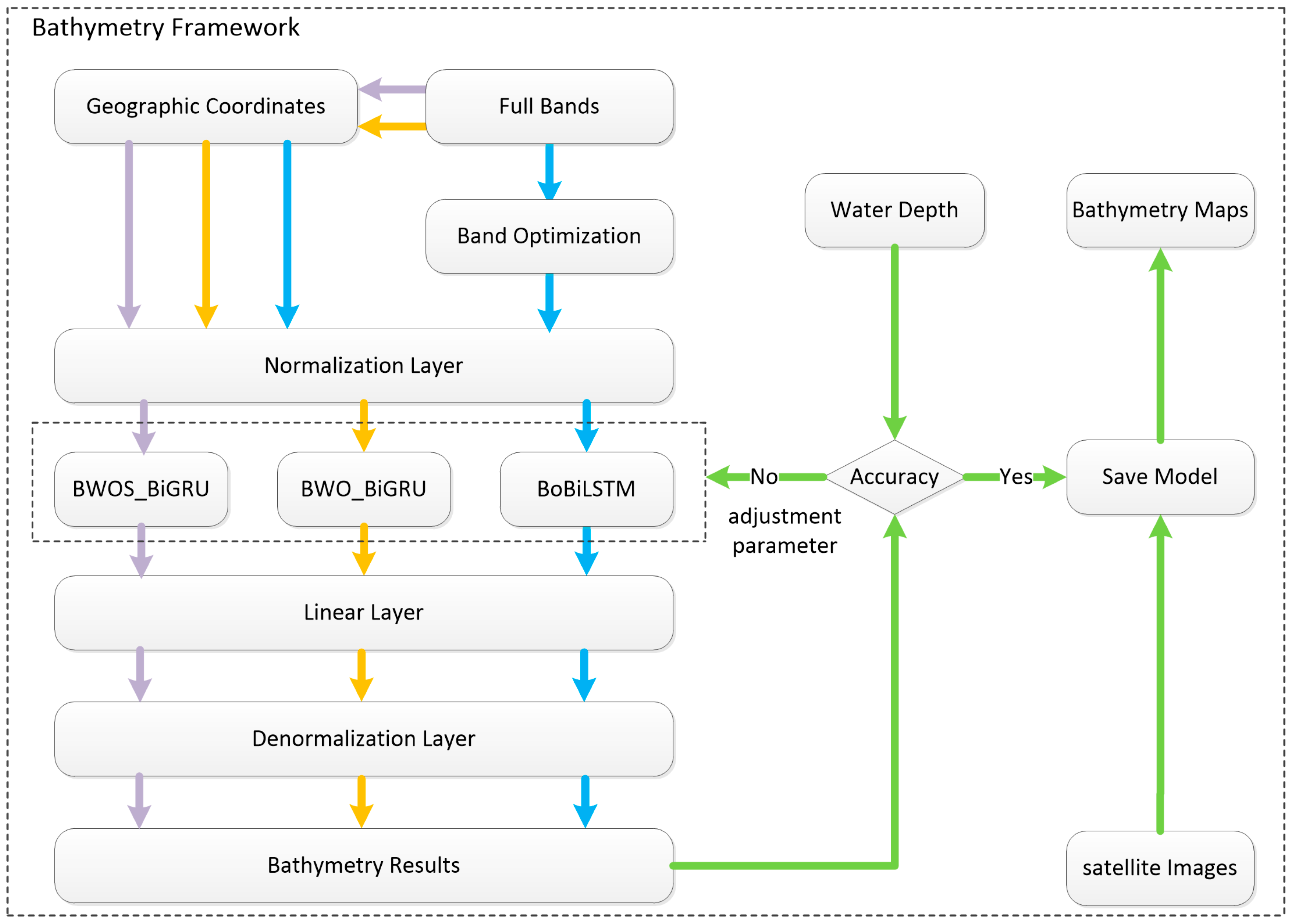
  • Bathymetry inversion framework
The blue, yellow, and purple arrows in Figure 5, respectively, represent the bathymetry inversion processes of the BoBiLSTM model, BWO_BiGRU model, and BWOS_BiGRU model. The green arrow indicates the process of validating the bathymetry inversion results of different models and generating bathymetry maps for large-area satellite images. The bathymetry framework consists of the data layer (all bands and geographic coordinates of different satellite images), band selection layer, normalization layer, model layer, linear layer, denormalization layer, and result layer. The band selection layer is a unique method of the BoBiLSTM model. Before participating in bathymetry inversion, the BoBiLSTM model must first perform the computation of the band selection layer. The normalization layer and denormalization layer are set to accelerate the convergence speed of the deep learning model. The linear layer is a method used by the deep learning model to handle regression problems. The result layer involves comparing the bathymetry inversion results of different deep learning models with the reference water depth extracted from ICESat-2 for validation. The model with higher accuracy is saved as the final bathymetry inversion model, which is then loaded to generate bathymetry maps from satellite images. From Figure 5, it can be observed that BWO_BiGRU and BWOS_BiGRU models can replace the band selection layer of the BoBiLSTM model, thereby improving the computational efficiency of the model. The parameter settings for the deep learning models are shown in Table 3.

2.3.4. Evaluation of Model Performance

This study uses the Stumpf model, BoBiLSTM model, BWO_BiGRU model, and BWOS_BiGRU model to analyze the SDB accuracy and performance of EnMAP, Sentinel2, and Landsat9, respectively. Each model corresponds to three types of satellite images and ICESat-2 data sources, and the indicators used are coefficient of determination (R2) and root mean square error (RMSE).

3. Results

3.1. Bathymetry Inversion Using Different Satellite Images

3.1.1. Correction Results of ICESat-2 Data

By using the method in Section 2.2.4, more than 310,000 bathymetry points were obtained from 17 strips of photon data. Table 4 lists the amount of data collected and the minimum and maximum water depth before and after correction of each ATL03 strip. The water depth range of ATL03 in the study area is concentrated from 0.344 m to 10.784 m. Previous studies [68,69] used certain pieces of ATL03 data as the training data for the model and other pieces as test data for the model. However, when measuring depth with laser pulses, there are certain differences between the shallow-water area and deep-water area of each piece of ATL03 data. The screening process also needs to consider whether the training dataset contains the characteristic values of all bathymetry points in the study area as much as possible. On the other hand, using a large amount of ATL03 data as the training data not only increases the running time of the model but also reduces the efficiency of the model. In practical applications, not all research areas can collect dense ATL03 data. Therefore, this study used a random function to randomly select less than 50,000 points from 310,000 bathymetry points, with the water depth ranging from 0.344 m to 10.784 m, and then used the random function again to make 30,000 points as the training data and 20,000 points as test data for the model. The ratio of the data size of the training set to the test set is 3:2. The bathymetry points filtered in this way cannot only include the bathymetry range of the study area but also test the ability of different models to draw bathymetry inversion maps for large areas by satellites.

3.1.2. Bathymetry Inversion from Different Satellite Images

Twelve types of bathymetry inversion results were generated using three types of satellite images and four different bathymetry inversion models (shown in Table 5). For EnMAP images, there are missing bands in the near-red and near-infrared bands. The Stumpf model only uses 2 (band 29 and band 35) of the first 46 bands of VNIR in estimating water depth, and the spectrum ranges from 420 nm to 650 nm. Bathymetry inversion results of the Stumpf model are the lowest compared to the other three deep learning models, with R2 being 0.89 and RMSE being 0.79 m. The BoBiLSTM model selected 19 bands and 2 band ratios for bathymetry inversion, with R2 being 0.93 and RMSE being 0.64 m. Among them, bands 1, 2, 3, 4, and 6 are coastal blue bands, accounting for 8% of the importance of water depth; band 18 is the blue band and accounts for 0.5% of the importance of water depth; bands 29, 35, 37, and 38 are green bands and account for 25% of the importance of water depth; bands 39, 42, 43, 44, 45, 46, and 47 are red bands, accounting for 57.6% of the importance of water depth; bands 52 and 53 are near-infrared bands and account for 2.8% of the importance of water depth. The BWO_BiGRU model uses 67 bands of VNIR, and its R2 and RMSE are comparable to the BoBiLSTM model. Compared with the BoBiLSTM model, this model also counts bands whose importance in bathymetry inversion is less than 10%. The BWOS_BiGRU model uses the 67 bands of VNIR and the band ratio of the Stumpf model. Compared with the other two deep learning models, the R2 and RMSE of this model are 0.93 and 0.63 m respectively, which slightly improves the bathymetry inversion accuracy.
For Sentinel-2 images, the Stumpf model has the worst bathymetry inversion effect compared to the other three deep learning models, with R2 of 0.66 and RMSE of 1.41 m. The bathymetry inversion effects of the BoBiLSTM model and the BWO_BiGRU model are equivalent, with R2 both being 0.91 and RMSE both being 0.72 m. In the BoBiLSTM model, band 2 is the blue band, accounting for 4% of the importance of water depth; band 3 is the green band, accounting for 5% of the importance of water depth; band 4 is the red band, accounting for 76% of the importance of water depth; band 9 is the water vapor band, accounting for 5% of the importance of water depth. The BWOS_BiGRU model uses 11 bands and 1 band ratio. Compared with the other two deep learning models, the R2 and RMSE of this model are 0.91 and 0.70 m respectively, which slightly improves the bathymetry inversion accuracy. For Landsat 9 images, the bathymetry inversion accuracy of the Stumpf model is the lowest among all models, with R2 only 0.54 and RMSE 1.64 m. The correlations of the bathymetry inversion of the other three deep learning models are all above 0.89. In the BoBiLSTM model, band 2 is a blue band, accounting for 3% of the importance of water depth; band 3 is a green band, accounting for 24% of the importance of water depth; band 4 is a red band, accounting for 66% of the importance of water depth. The BWO_BiGRU model uses 8 bands, of which R2 and RMSE are 0.91 and 0.71 m, respectively. Its accuracy is slightly higher than the BoBiLSTM model. The BWOS_BiGRU model uses 8 bands and 1 band ratio, among which the RMSE is the lowest at 0.69 m compared with the other three models.
Comparing the accuracy of twelve bathymetry inversions, the model with the best effect using hyperspectral image EnMAP is BWOS_BiGRU. For multispectral images of Sentinel-2 and Landsat 9, the BoBiLSTM model, BWO_BiGRU model, and BWOS_BiGRU model can all improve the accuracy of bathymetry inversion, but the effect is slightly lower than that of EnMAP images. As can be seen from Figure 6, The bathymetry inversion effect of the Stumpf model is better in EnMAP images (Figure 6a), with the maximum inversion depth reaching about 9 m; while the effect in Sentinel-2 and Landsat 9 images (Figure 6e,i) is very poor, in which most of the bathymetry points are scattered on both sides away from the red trend line and the maximum inversion accuracy is around 8 m. The data volume of the test set is as high as more than 20,000 points, when there are enough eigenvalues in different bands, the deep learning model can learn more feature importance related to water depth, so the effect of bathymetry inversion on the test set performs very well. Whether it is a hyperspectral image or a multispectral image, the BoBiLSTM model (Figure 6b–d), BWO_BiGRU model (Figure 6f–h), and BWOS_BiGRU model (Figure 6j–l) can all invert water depth to about 10 m. Most of bathymetry points of these models are concentrated near the red trend line, among which the BWOS_BiGRU model has the lowest RMSE.
The bathymetry inversion maps generated by different models using EnMAP, Sentinel-2, and Landsat 9 images are shown in Figure 7. The isobaths of different bathymetry inversion maps are spaced at 2 m intervals and relatively smooth. The Stumpf model demonstrates a bathymetry inversion range of 0 to 7 m on the EnMAP image (Figure 7a), exhibiting a good bathymetry texture. However, the water depth in deep areas is underestimated. On the Sentinel-2 image (Figure 7e), a bathymetry inversion range of this model is 0 to 15 m, with water depths exceeding 10 m in the transition zone between deep and shallow areas. The texture transition in bathymetry inversion also appears relatively coarse. The bathymetry inversion range of this model on the Landsat 9 image (Figure 7i) is 0 to 6 m, with the bathymetry texture showing deeper water in shallow areas and shallower water in deep areas. The BoBiLSTM model exhibits a bathymetry inversion range of 0 to 15 m on the EnMAP image (Figure 7b). The bathymetry transition between shallow and deep areas appears relatively smooth, but the model tends to predict shallower-water depths in areas with depths exceeding 7 m. On the Sentinel-2 image (Figure 7f) and Landsat 9 image (Figure 7j), the bathymetry inversion range of this model is both 0 to 8 m. In both cases, there is a tendency to underestimate water depths in deep areas exceeding 6 m, with the Landsat 9 image showing cases of overestimation in the nearshore shallow-water areas. The BWO_BiGRU model (Figure 7c) and BWOS_BiGRU model (Figure 7d) both demonstrate a bathymetry inversion range of 0 to 13 m on the EnMAP image. The bathymetry texture exhibits smooth transitions, whether in shallow or deep areas, and the fluctuations in water depth appear natural. The bathymetry inversion performance of these two models on the EnMAP image is superior to that of the Stumpf model (Figure 7a) and BoBiLSTM model (Figure 7b). On the Sentinel-2 image, the BWO_BiGRU model (Figure 7g) exhibits a bathymetry inversion range of 0 to 11 m, with a tendency to underestimate water depths in deep areas. Meanwhile, the bathymetry inversion range of the BWOS_BiGRU model (Figure 7h) is 0 to 8 m, underestimating areas with water depths greater than 7 m. The bathymetry inversion performance of the BWOS_BiGRU model is slightly lower than that of the BWO_BiGRU model (Figure 7g). On the Landsat 9 image, the BWO_BiGRU model (Figure 7k) shows a bathymetry inversion range of 0 to 15 m, significantly overestimating water depths in deep areas and underestimating water depths in shallow areas. In contrast, the BWOS_BiGRU model (Figure 7l) exhibits a bathymetry inversion range of 0 to 13 m, with a tendency to underestimate water depths in deep areas. In summary, the models that demonstrate superior performance in bathymetry inversion using EnMAP imagery are the BWO_BiGRU and BWOS_BiGRU models. For bathymetry inversion using Sentinel-2 imagery, the BWO_BiGRU model stands out. When it comes to bathymetry inversion using Landsat 9 imagery, the BWOS_BiGRU model excels in shallow-water areas, while the BoBiLSTM model performs well in deep-water areas. It is noteworthy that the performance of bathymetry inversion using EnMAP imagery is consistently better than that achieved with Sentinel-2 and Landsat 9 imagery.

3.2. Effect Analysis of Bathymetry Inversion

To analyze the bathymetry inversion effects of different satellite images, comparisons were made among different models based on their RMSE across various water depth intervals, as depicted in Table 6. In model training and testing, we used fewer than 50,000 ICESat-2 bathymetry points, of which only 29 points had a depth greater than 10 m, accounting for approximately 0.06% of the data. As a result, deep learning models exhibited significant errors when predicting water depths above this threshold, with an RMSE value exceeding 4 m. This indicates that the performance of deep learning models in bathymetry inversion is poor when the dataset is insufficient. In contrast, the Stumpf model, being a linear model, shows lower errors with an RMSE of 2.78 m. This implies that all models have limited accuracy in predicting water depths exceeding 10 m. When using EnMAP imagery, the BWO_BiGRU model and the BWOS_BiGRU model perform best within the water depth interval of 6 to 8 m, with RMSE values around 0.45 m. The second-best performance is observed in the interval of 4 to 6 m, with RMSE values around 0.6 m. The third-best performance is in the intervals of 2 to 4 m and 8 to 10 m, with RMSE values around 0.7 m. The least accurate predictions are in the shallow-water range of 0 to 2 m, with RMSE values around 0.8 m. This is also consistent with the actual ICESat-2 data collected, where the majority of bathymetry points are concentrated within the range of 2 to 10 m. The more data points there are within each water depth interval, the more feature importance the deep learning model learns, resulting in smaller RMSE values. When using Sentinel-2 and Landsat 9 imagery, the BWO_BiGRU model and the BWOS_BiGRU model exhibit slightly increased RMSE values across different water depth intervals compared to EnMAP imagery. The BoBiLSTM model generally shows higher RMSE values across various water depth intervals compared to the BWO_BiGRU and BWOS_BiGRU models. The Stumpf model performs the worst, with RMSE values exceeding 2 m in the 0 to 2 m water depth interval.
Figure 8 presents the residual maps of different models using various satellite images for bathymetry inversion. For the BoBiLSTM, BWO_BiGRU, and BWOS_BiGRU models, over 90% of the residual distribution for predicted bathymetry points is concentrated within 1 m. Among them, the performance of EnMAP imagery surpasses that of Sentinel-2 and Landsat 9 imagery. In EnMAP imagery, the Stumpf model exhibits 85% of the residuals distributed within 1 m, while its performance is less favorable in Sentinel-2 and Landsat 9 imagery, with less than 60% of residuals distributed within 1 m. Therefore, combining deep learning models with hyperspectral satellite imagery enhances the accuracy of bathymetry inversion.
This study selected the bathymetry data from two ATL03 data (20210626GT1R and 20201215GT3L) for the study area and compared the bathymetry profiles predicted by different models, as shown in Figure 9. The 20210626GT1R track data cover approximately 63 km, while the 20201215GT3L track data cover around 40 km. Both datasets encompass shallow and deep-water regions. Through comparative analysis, it can be observed that the depth range predicted by the Stumpf model in the three types of imagery is around 5 m. In the EnMAP case, the bathymetry profiles of all deep learning models are fitted near the ATL03 data. Among them, the BWO_BiGRU model (Figure 9a) and BWOS_BiGRU model (Figure 9d) provide more accurate predictions for deep-water regions. In the Sentinel-2 case, the water depth profiles of all deep learning models (Figure 9b,e) closely match the ATL03 data in shallow water areas, with the BWO_BiGRU model providing a slightly better fit in deep-water regions. In the Landsat 9 case (Figure 9c,f), the bathymetry profile of the BoBiLSTM model can only predict depths of around 6 m in deep-water areas, but it predicts deeper depths in shallow-water areas. The bathymetry profile of the BWO_BiGRU model is deeper, while the profile of the BWOS_BiGRU model fits well in shallow-water areas but is slightly shallower in deep-water regions. Comparing the bathymetry profiles generated from different images, it is evident that the transition of bathymetry textures in both shallow and deep-water areas is superior in EnMAP imagery compared to Sentinel-2 and Landsat 9.

4. Discussion

This paper proposes a BWO_BiGRU model that optimizes the weights of all bands in satellite images. The model eliminates the need for band selection for different images and can directly assign varying feature importance to bands that impact bathymetry changes through the self-attention mechanism during the training process. On the other hand, this method focuses on the spectral characteristics of neighboring pixels in the imagery, and even if some spectral bands are missing, it does not significantly degrade the accuracy of bathymetric inversion. The BWOS_BiGRU model, on the basis of a band weight-optimized algorithm, adds a band ratio from the Stumpf model. This method does not have a significant impact on the bathymetry inversion results for EnMAP images (Figure 7c,d), but it has a considerable impact on the results for Sentinel-2 images (Figure 8g,h) and Landsat 9 images (Figure 7k,l). Due to the high number of bands and narrow spectral range in hyperspectral images, the feature importance carried by these bands has already sensitively captured the rules of water depth fluctuations. Therefore, the contribution of water depth from the band ratios of the Stumpf model is relatively small compared to all the bands. For multispectral images, the main bands influencing bathymetry inversion are concentrated in the red, green, and blue bands, each with a broad spectral range. The importance of bathymetry features carried by each band is not prominently emphasized due to the large amount of information. Therefore, by adding the band ratios of the Stumpf model, the BWOS_BiGRU model affects the bathymetry inversion results by introducing an additional important feature. Additionally, by comparing the spectral ranges of Sentinel-2 and Landsat 9 in Table 1, it can be observed that Landsat 9 has broader spectral ranges for each band with larger intervals between adjacent bands. Therefore, in the BWO_BiGRU model, the bathymetric inversion results for Sentinel-2 imagery (Figure 7g) outperform those for Landsat 9 imagery (Figure 7k). The bathymetry inversion map generated in this study covers over two million points, involving the synthesis of multiple satellite images with a considerable amount of spectral feature information. Consequently, the performance of the Stumpf model in bathymetry inversion is generally mediocre in EnMAP images and very poor in Sentinel-2 and Landsat 9 images. For bathymetry inversion using the BoBiLSTM model, it is necessary to prioritize the consideration of different spectral features from multiple images. This involves manually inspecting the missing values in various bands and evaluating them before selecting the relevant features. This process is relatively complex, as the selection of spectral features directly influences the accuracy of bathymetry inversion. Therefore, this model is more suitable for generating bathymetry inversion maps based on a single image. Although BoBiLSTM makes full use of the spectral information of the 90% most important features, this study indicates that it is still not possible to ignore other spectral bands contributing less than 10% when constructing large-area bathymetry maps. These additional bands contribute to higher accuracy in bathymetric inversion. In the data preprocessing stage, the BWO_BiGRU and BWOS_BiGRU models do not require band feature selection. During large-scale bathymetry inversion, the models will fully learn the interdependencies between the bands in the images, assigning higher weights to the bands that contribute significantly to bathymetry inversion, thereby obtaining more effective bathymetry information. In comparison to BoBiLSTM, these models can offer higher accuracy in bathymetry inversion and are more suitable for generating large-area bathymetry maps using multiple images from hyperspectral satellites.
The model proposed in this paper establishes a nonlinear mapping relationship between the spectral range of the image and water depth, focusing on analyzing the differences in bathymetry inversion between multispectral and hyperspectral spectra. In bathymetry inversion, the quality of satellite images and the water quality in the study area have a significant impact on the model, while the time of data acquisition has no effect on the model. Additionally, we conducted refraction correction and tidal correction on the collected ICESat-2 water depth data, which can improve the accuracy of bathymetry inversion. In this study, the application of the RANSAC method to extract ICESat-2 bathymetry points represents a novel approach. The sampling interval of ATL03 data along the orbit is 70 cm, while the spatial resolution of various satellite images is 30 m. Consequently, laser pulses scanning the seafloor can generate multiple bathymetry points with different elevations or the same elevation within a single pixel. When there is a large amount of bathymetry data, the trend line of water depth can be represented by a polyline instead of a curve to describe the undulating changes in seafloor topography. This fitting process may result in data loss, and as a result, the Stumpf model does not perform well in bathymetry inversion on multispectral satellite images. The BoBiLSTM model focuses on selecting band features, removing bands that have a minimal impact on bathymetry inversion from hyperspectral or multispectral images. For smaller study areas, the decrease in depth accuracy may not be very significant, but for larger water bodies, the depth accuracy notably declines. Therefore, utilizing information from all effective bands is crucial. In contrast, deep learning models proposed in this paper, while learning the correlation between spectral reflectance features and water depth, can tolerate bathymetry data with larger errors. Therefore, the performance of bathymetry inversion is better on hyperspectral or multispectral images. The VNIR channels of hyperspectral images have the advantage of a large number of bands with relatively narrow spectral ranges. Fully utilizing these characteristics can improve the accuracy of bathymetry inversion. However, it is important to consider the available spectral range of hyperspectral images and the relative loss of bands. If the bands that contribute significantly to bathymetry inversion are lost more, the accuracy of the bathymetry inversion from hyperspectral images will also decrease. Multispectral images, which have achieved global coverage, may offer slightly lower bathymetry inversion accuracy compared to hyperspectral images. However, by selecting appropriate bathymetry inversion methods, global shallow water monitoring can be realized. Furthermore, Sentinel-2 offers visible light bands with a 10 m resolution, which provides an opportunity for further research on shoreline changes through multi-temporal multispectral image-based bathymetry monitoring. Comparing different models for generating bathymetric maps from various satellite images, the BWO_BiGRU model and RANSAC-based method for extracting ICESat-2 bathymetric points are more suitable for generating large-area bathymetry maps using hyperspectral satellites, while the BWOS_BiGRU model and RANSAC-based method are more suitable for generating large-area bathymetry maps in shallow-water areas (0–5 m) using multispectral satellites.
This study additionally downloads DEM data of Shark Bay [70], as shown in Figure 10a. The spatial resolution of the raster data is 10 m. Figure 10b is a bathymetry map generated by using EnMAP images and the BWO_BiGRU model. Its bathymetry texture features are similar to those of Figure 10a, with an RMSE of 1.19 m. The proposed model is lightweight and practical, demonstrating outstanding performance and accuracy in extracting depths from large shallow marine areas. In [71,72], most studies use field methods such as multi-beam or single-beam to collect water depth data, combined with traditional empirical models like Stumpf and remote sensing images to perform water depth inversion for the study area. These methods typically require a long time period to study shallow-water areas with missing data. In contrast, the method proposed in this paper can obtain water depth values with a certain degree of accuracy over a large area in a short period of time. Additionally, by taking advantage of the short revisit cycle of ICESat-2, it is possible to measure the water depth of the same water body at different times, allowing for the comparison and validation of depth measurement results. This is of great significance for long-term studies on the water depth variations of a specific water body. Therefore, the bathymetric map generated using the method proposed in this paper can provide data support for global shallow marine environment mapping. The profiles of different deep learning models, ICESat-2 reference data source (ATL03 20220613GT1R strip data with a length of about 59 km), and Shark Bay DEM were compared under different satellite images, as shown in Figure 11. The effect of the bathymetry profile line in the EnMAP image is better than that of the Sentinel-2 and Landsat 9 images. The bathymetry trend of the ICESat-2 20220613GT1R track is similar to the reference bathymetry profile of Shark Bay, indicating the effectiveness of the RANSAC method in extracting valid bathymetry photons in large water areas. By comparison, the profile line obtained by using the EnMAP image and the BWO_BiGRU model to generate the bathymetry map (Figure 11a orange line) fits better with the 20220613GT1R track (Figure 11a red line) and the Shark Bay reference bathymetry profile (Figure 11a purple line), demonstrating that the method proposed in this paper is suitable for bathymetry inversion in large water areas. This is of great significance for filling in the bathymetry of blank areas and can provide a more convenient and widely applicable method for marine engineering in practical environments. Our research can also be further explored in real-time applications. For example, during the data preprocessing stage, the RANSAC method can be encapsulated into an application to directly process bathymetry data points of ICESat-2. The BWO_BiGRU model can be integrated for training, testing, and inference to provide an end-to-end service, making it more convenient for practical production applications.

5. Conclusions

This study proposes a method for large-area bathymetry inversion of satellite images (EnMAP, Landsat 9, and Sentinel-2) using the BWO_BiGRU model and RANSAC method for extracting bathymetry points of ICESat-2. This model optimizes information from all spectral bands of satellite images, assigning distinct weight information to different bands. Additionally, bidirectional encoding of the model further enhances information features of both shallow and deep-water areas, contributing to improved accuracy in bathymetry inversion. Furthermore, using the RANSAC method for clustering ICESat-2 data can expedite data convergence and effectively separate photon data from the sea surface and seabed. Building on these studies, the BWOS_BiGRU model is further proposed. In its input phase, it incorporates not only the full spectral data but also a band ratio from the Stumpf model. This addition is aimed at enhancing the bathymetry inversion of multispectral satellite images, particularly in shallow-water areas, during the model training process. A series of experiments in the Shark Bay region of Western Australia indicate that the accuracy of bathymetry inversion using the BWO_BiGRU model and BWOS_BiGRU model applied to EnMAP imagery is superior to other models. The RMSEs for these models are 0.64 m and 0.63 m, respectively, which are lower than those for Sentinel-2 imagery (RMSEs of 0.72 m and 0.70 m) and Landsat 9 imagery (RMSEs of 0.71 m and 0.69 m). The water area in the study region is relatively large, approximately 1725 km2. The comparable performance of the BWOS_BiGRU model and the BWO_BiGRU model applied to EnMap imagery in bathymetry inversion demonstrates that hyperspectral imagery can achieve good results in bathymetry inversion without the need for additional band features. This further emphasizes the superior capability of hyperspectra imagery over multispectral imagery in large-area bathymetry mapping. Compared with the Stumpf and BoBiLSTM models, the BWO_BiGRU model proposed in this study does not require band selection in the data preprocessing stage and is more suitable for bathymetry inversion of large areas involving the synthesis of multiple images in hyperspectral satellite images. Additionally, the BWOS_BiGRU model exhibits better convergence for bathymetry in shallow-water areas (0–5 m) in multispectral satellite images. In future research, further exploration will be conducted to enhance the accuracy of bathymetry inversion in different water bodies using various satellite images. Efforts will also be directed towards improving the robustness of hyperspectral images and existing models in diverse scenarios, aiming to unlock additional potential applications such as distribution of coral reef and underwater terrain mapping.

Author Contributions

Data curation, experiment analysis, writing—original draft preparation, X.X.; Conceptualization, methodology, supervision, writing—review and editing, G.G.; investigation, validation, visualization, G.G. and J.G. All authors have read and agreed to the published version of the manuscript.

Funding

This research received no external funding.

Institutional Review Board Statement

Not applicable.

Data Availability Statement

ICESat data can be obtained through the website https://nsidc.org/data/atl03/versions/5 (accessed on 5 October 2023). The EnMAP image can be obtained through the website https://www.enmap.org/ (accessed on 20 October 2023). The Sentinel-2 image can be obtained through the website https://scihub.copernicus.eu/dhus/#/home (accessed on 12 October 2023). The Landsat 9 image can be obtained through the website https://earthexplorer.usgs.gov/ (accessed on 12 October 2023). The DEM can be obtained through the website https://doi.org/10.25919/pwfr-mk06 (accessed on 12 July 2024).

Acknowledgments

The authors express sincere appreciation for the following organizations, NASA (National Aeronautics and Space Administration), DLR (German Aerospace Center), ESA (European Space Agency), USGS (United States Geological Survey) and CSIRO (Commonwealth Scientific and Industrial Research Organisation), for providing ICESat-2, EnMAP, Sentinel-2, Landsat 9, and DEM data, respectively.

Conflicts of Interest

The authors declare no conflicts of interest.

References

  1. Cui, X.; Xing, Z.; Yang, F.; Fan, M.; Ma, Y.; Sun, Y. A Method for Multibeam Seafloor Terrain Classification Based on Self-Adaptive Geographic Classification Unit. Appl. Acoust. 2020, 157, 107029. [Google Scholar] [CrossRef]
  2. Asner, G.P.; Vaughn, N.R.; Balzotti, C.; Brodrick, P.G.; Heckler, J. High-Resolution Reef Bathymetry and Coral Habitat Complexity from Airborne Imaging Spectroscopy. Remote Sens. 2020, 12, 310. [Google Scholar] [CrossRef]
  3. Lecours, V.; Dolan, M.F.J.; Micallef, A.; Lucieer, V.L. A Review of Marine Geomorphometry, the Quantitative Study of the Seafloor. Hydrol. Earth Syst. Sci. 2016, 20, 3207–3244. [Google Scholar] [CrossRef]
  4. Virtasalo, J.J.; Korpinen, S.; Kotilainen, A.T. Assessment of the Influence of Dredge Spoil Dumping on the Seafloor Geological Integrity. Front. Mar. Sci. 2018, 5, 131. [Google Scholar] [CrossRef]
  5. Hedley, J.; Roelfsema, C.; Chollett, I.; Harborne, A.; Heron, S.; Weeks, S.; Skirving, W.; Strong, A.; Eakin, C.; Christensen, T.; et al. Remote Sensing of Coral Reefs for Monitoring and Management: A Review. Remote Sens. 2016, 8, 118. [Google Scholar] [CrossRef]
  6. Mestdagh, S.; Amiri-Simkooei, A.; van der Reijden, K.J.; Koop, L.; O’Flynn, S.; Snellen, M.; Van Sluis, C.; Govers, L.L.; Simons, D.G.; Herman, P.M.J.; et al. Linking the Morphology and Ecology of Subtidal Soft-Bottom Marine Benthic Habitats: A Novel Multiscale Approach. Estuar. Coast. Shelf Sci. 2020, 238, 106687. [Google Scholar] [CrossRef]
  7. Diesing, M.; Green, S.L.; Stephens, D.; Lark, R.M.; Stewart, H.A.; Dove, D. Mapping Seabed Sediments: Comparison of Manual, Geostatistical, Object-Based Image Analysis and Machine Learning Approaches. Cont. Shelf Res. 2014, 84, 107–119. [Google Scholar] [CrossRef]
  8. Dietrich, J.T. Bathymetric Structure-from-Motion: Extracting Shallow Stream Bathymetry from Multi-View Stereo Photogrammetry. Earth Surf. Process. Landf. 2016, 42, 355–364. [Google Scholar] [CrossRef]
  9. Cao, B.; Fang, Y.; Jiang, Z.; Gao, L.; Hu, H. Shallow Water Bathymetry from WorldView-2 Stereo Imagery Using Two-Media Photogrammetry. Eur. J. Remote Sens. 2019, 52, 506–521. [Google Scholar] [CrossRef]
  10. Zhou, Y.; Lu, L.; Li, L.; Zhang, Q.; Zhang, P. A Generic Method to Derive Coastal Bathymetry from Satellite Photogrammetry for Tsunami Hazard Assessment. Geophys. Res. Lett. 2021, 48, e2021GL095142. [Google Scholar] [CrossRef]
  11. Popielarczyk, D. Determination of Survey Boat “Heave” Motion with the Use of RTS Technique. In Proceedings of the 10th International Conference “Environmental Engineering”, Vilnius, Lithuania, 27–28 April 2017. [Google Scholar]
  12. Rowley, T.; Ursic, M.; Konsoer, K.; Langendoen, E.; Mutschler, M.; Sampey, J.; Pocwiardowski, P. Comparison of Terrestrial Lidar, SfM, and MBES Resolution and Accuracy for Geomorphic Analyses in Physical Systems that Experience Subaerial and Subaqueous Conditions. Geomorphology 2020, 355, 107056. [Google Scholar] [CrossRef]
  13. Borrelli, M.; Legare, B.; McCormack, B.; dos Santos, P.P.G.M.; Solazzo, D. Absolute Localization of Targets Using a Phase-Measuring Sidescan Sonar in Very Shallow Waters. Remote Sens. 2023, 15, 1626. [Google Scholar] [CrossRef]
  14. Pessanha, V.S.; Chu, P.C.; Gough, M.K.; Orescanin, M.M. Coupled Model to Predict Wave-Induced Liquefaction and Morphological Changes. J. Sea Res. 2023, 192, 102351. [Google Scholar] [CrossRef]
  15. Ghorbanidehno, H.; Lee, J.; Farthing, M.; Hesser, T.; Kitanidis, P.K.; Darve, E.F. Novel Data Assimilation Algorithm for Nearshore Bathymetry. J. Atmos. Ocean. Technol. 2019, 36, 699–715. [Google Scholar] [CrossRef]
  16. Wu, J.; Hao, X.; Li, T.; Shen, L. Adjoint-Based High-Order Spectral Method of Wave Simulation for Coastal Bathymetry Reconstruction. J. Fluid Mech. 2023, 972, A41. [Google Scholar] [CrossRef]
  17. Danilo, C.; Melgani, F. Wave Period and Coastal Bathymetry Using Wave Propagation on Optical Images. IEEE Trans. Geosci. Remote Sens. 2016, 54, 6307–6319. [Google Scholar] [CrossRef]
  18. Wei, Z.; Guo, J.; Zhu, C.; Yuan, J.; Chang, X.; Ji, B. Evaluating Accuracy of HY-2A/GM-Derived Gravity Data with the Gravity-Geologic Method to Predict Bathymetry. Front. Earth Sci. 2021, 9, 636246. [Google Scholar] [CrossRef]
  19. Sun, Y.; Zheng, W.; Li, Z.; Zhou, Z. Improved the Accuracy of Seafloor Topography from Altimetry-Derived Gravity by the Topography Constraint Factor Weight Optimization Method. Remote Sens. 2021, 13, 2277. [Google Scholar] [CrossRef]
  20. Hsiao, Y.-S.; Hwang, C.; Cheng, Y.-S.; Chen, L.-C.; Hsu, H.-J.; Tsai, J.-H.; Liu, C.-L.; Wang, C.-C.; Liu, Y.-C.; Kao, Y.-C. High-Resolution Depth and Coastline Over Major Atolls of South China Sea from Satellite Altimetry and Imagery. Remote Sens. Environ. 2016, 176, 69–83. [Google Scholar] [CrossRef]
  21. Xing, S.; Wang, D.; Xu, Q.; Lin, Y.; Li, P.; Liu, C. Characteristic Analysis of the Green-Channel Waveforms with ALB Mapper5000. In Proceedings of the 2019 IEEE International Conference on Signal, Information and Data Processing (ICSIDP), Chongqing, China, 11–13 December 2019; pp. 1–4. [Google Scholar]
  22. Szafarczyk, A.; Tos, C. The Use of Green Laser in LiDAR Bathymetry: State of the Art and Recent Advancements. Sensors 2022, 23, 292. [Google Scholar] [CrossRef] [PubMed]
  23. Guo, K.; Xu, W.; Liu, Y.; He, X.; Tian, Z. Gaussian Half-Wavelength Progressive Decomposition Method for Waveform Processing of Airborne Laser Bathymetry. Remote Sens. 2017, 10, 35. [Google Scholar] [CrossRef]
  24. Huang, L.; Meng, J.; Fan, C.; Zhang, J.; Yang, J. Shallow Sea Topography Detection from Multi-Source SAR Satellites: A Case Study of Dazhou Island in China. Remote Sens. 2022, 14, 5184. [Google Scholar] [CrossRef]
  25. Bian, X.; Shao, Y.; Zhang, C.; Xie, C.; Tian, W. The Feasibility of Assessing Swell-Based Bathymetry Using SAR Imagery from Orbiting Satellites. ISPRS J. Photogramm. Remote Sens. 2020, 168, 124–130. [Google Scholar] [CrossRef]
  26. Han, T.; Zhang, H.; Cao, W.; Le, C.; Wang, C.; Yang, X.; Ma, Y.; Li, D.; Wang, J.; Lou, X. Cost-Efficient Bathymetric Mapping Method Based on Massive Active–Passive Remote Sensing Data. ISPRS J. Photogramm. Remote Sens. 2023, 203, 285–300. [Google Scholar] [CrossRef]
  27. Gabr, B.; Ahmed, M.; Marmoush, Y. PlanetScope and Landsat 8 Imageries for Bathymetry Mapping. J. Mar. Sci. Eng. 2020, 8, 143. [Google Scholar] [CrossRef]
  28. Zhang, H.; Ma, Y.; Zhang, J.; Zhao, X.; Zhang, X.; Leng, Z. Atmospheric Correction Model for Water–Land Boundary Adjacency Effects in Landsat-8 Multispectral Images and Its Impact on Bathymetric Remote Sensing. Remote Sens. 2022, 14, 4769. [Google Scholar] [CrossRef]
  29. Niroumand-Jadidi, M.; Legleiter, C.J.; Bovolo, F. River Bathymetry Retrieval from Landsat-9 Images Based on Neural Networks and Comparison to SuperDove and Sentinel-2. IEEE J. Sel. Top. Appl. Earth Obs. Remote Sens. 2022, 15, 5250–5260. [Google Scholar] [CrossRef]
  30. Bergsma, E.W.J.; Almar, R.; Maisongrande, P. Radon-Augmented Sentinel-2 Satellite Imagery to Derive Wave-Patterns and Regional Bathymetry. Remote Sens. 2019, 11, 1918. [Google Scholar] [CrossRef]
  31. Babbel, B.J.; Parrish, C.E.; Magruder, L.A. ICESat-2 Elevation Retrievals in Support of Satellite-Derived Bathymetry for Global Science Applications. Geophys. Res. Lett. 2021, 48, e2020GL090629. [Google Scholar] [CrossRef]
  32. Granadeiro, J.P.; Belo, J.; Henriques, M.; Catalão, J.; Catry, T. Using Sentinel-2 Images to Estimate Topography, Tidal-Stage Lags and Exposure Periods over Large Intertidal Areas. Remote Sens. 2021, 13, 320. [Google Scholar] [CrossRef]
  33. Cheng, L.; Ma, L.; Cai, W.; Tong, L.; Li, M.; Du, P. Integration of Hyperspectral Imagery and Sparse Sonar Data for Shallow Water Bathymetry Mapping. IEEE Trans. Geosci. Remote Sens. 2015, 53, 3235–3249. [Google Scholar] [CrossRef]
  34. Ma, S.; Tao, Z.; Yang, X.; Yu, Y.; Zhou, X.; Li, Z. Bathymetry Retrieval from Hyperspectral Remote Sensing Data in Optical-Shallow Water. IEEE Trans. Geosci. Remote Sens. 2014, 52, 1205–1212. [Google Scholar] [CrossRef]
  35. Alevizos, E. A Combined Machine Learning and Residual Analysis Approach for Improved Retrieval of Shallow Bathymetry from Hyperspectral Imagery and Sparse Ground Truth Data. Remote Sens. 2020, 12, 3489. [Google Scholar] [CrossRef]
  36. Niroumand-Jadidi, M.; Bovolo, F.; Bruzzone, L. Water Quality Retrieval from PRISMA Hyperspectral Images: First Experience in a Turbid Lake and Comparison with Sentinel-2. Remote Sens. 2020, 12, 3984. [Google Scholar] [CrossRef]
  37. Braga, F.; Fabbretto, A.; Vanhellemont, Q.; Bresciani, M.; Giardino, C.; Scarpa, G.M.; Manfè, G.; Concha, J.A.; Brando, V.E. Assessment of PRISMA Water Reflectance Using Autonomous Hyperspectral Radiometry. ISPRS J. Photogramm. Remote Sens. 2022, 192, 99–114. [Google Scholar] [CrossRef]
  38. Alevizos, E.; Le Bas, T.; Alexakis, D.D. Assessment of PRISMA Level-2 Hyperspectral Imagery for Large Scale Satellite-Derived Bathymetry Retrieval. Mar. Geod. 2022, 45, 251–273. [Google Scholar] [CrossRef]
  39. Minghelli, A.; Vadakke-Chanat, S.; Chami, M.; Guillaume, M.; Migne, E.; Grillas, P.; Boutron, O. Estimation of Bathymetry and Benthic Habitat Composition from Hyperspectral Remote Sensing Data (BIODIVERSITY) Using a Semi-Analytical Approach. Remote Sens. 2021, 13, 1999. [Google Scholar] [CrossRef]
  40. Minghelli, A.; Vadakke-Chanat, S.; Chami, M.; Guillaume, M.; Peirache, M. Benefit of the Potential Future Hyperspectral Satellite Sensor (BIODIVERSITY) for Improving the Determination of Water Column and Seabed Features in Coastal Zones. IEEE J. Sel. Top. Appl. Earth Obs. Remote Sens. 2021, 14, 1222–1232. [Google Scholar] [CrossRef]
  41. Becker, M.; Schreiner, S.; Auer, S.; Cerra, D.; Gege, P.; Bachmann, M.; Roitzsch, A.; Mitschke, U.; Middelmann, W. Reconnaissance of Coastal Areas Using Simulated EnMAP Data in an ERDAS IMAGINE Environment; SPIE: Bellingham, WA, USA, 2018; Volume 10790. [Google Scholar]
  42. Dörnhöfer, K.; Oppelt, N. Mapping Benthic Substrate Coverage and Bathymetry Using Bio-optical Modelling—An EnMAP Case Study in the Coastal Waters of Helgoland. In Proceedings of the 2014 6th Workshop on Hyperspectral Image and Signal Processing: Evolution in Remote Sensing (WHISPERS), Lausanne, Switzerland, 24–27 June 2014; pp. 1–6. [Google Scholar]
  43. Lyzenga, D.R. Shallow-Water Bathymetry Using Combined Lidar and Passive Multispectral Scanner Data. Int. J. Remote Sens. 1985, 6, 115–125. [Google Scholar] [CrossRef]
  44. Stumpf, R.P.; Holderied, K.; Sinclair, M. Determination of Water Depth with High-Resolution Satellite Imagery over Variable Bottom Types. Limnol. Oceanogr. 2003, 48, 547–556. [Google Scholar] [CrossRef]
  45. Lyzenga, D.R.; Malinas, N.P.; Tanis, F.J. Multispectral Bathymetry Using a Simple Physically Based Algorithm. IEEE Trans. Geosci. Remote Sens. 2006, 44, 2251–2259. [Google Scholar] [CrossRef]
  46. Najar, M.A.; Benshila, R.; Bennioui, Y.E.; Thoumyre, G.; Almar, R.; Bergsma, E.W.J.; Delvit, J.-M.; Wilson, D.G. Coastal Bathymetry Estimation from Sentinel-2 Satellite Imagery: Comparing Deep Learning and Physics-Based Approaches. Remote Sens. 2022, 14, 1196. [Google Scholar] [CrossRef]
  47. Ghorbanidehno, H.; Lee, J.; Farthing, M.; Hesser, T.; Darve, E.F.; Kitanidis, P.K. Deep Learning Technique for Fast Inference of Large-Scale Riverine Bathymetry. Adv. Water Resour. 2021, 147, 103715. [Google Scholar] [CrossRef]
  48. Yang, L.; Liu, M.; Liu, N.; Guo, J.; Lin, L.; Zhang, Y.; Du, X.; Xu, Y.; Zhu, C.; Wang, Y. Recovering Bathymetry from Satellite Altimetry-Derived Gravity by Fully Connected Deep Neural Network. IEEE Geosci. Remote Sens. Lett. 2023, 20, 1502805. [Google Scholar] [CrossRef]
  49. Misra, A.; Vojinovic, Z.; Ramakrishnan, B.; Luijendijk, A.; Ranasinghe, R. Shallow Water Bathymetry Mapping Using Support Vector Machine (SVM) Technique and Multispectral Imagery. Int. J. Remote Sens. 2018, 39, 4431–4450. [Google Scholar] [CrossRef]
  50. Sun, S.; Chen, Y.; Mu, L.; Le, Y.; Zhao, H. Improving Shallow Water Bathymetry Inversion through Nonlinear Transformation and Deep Convolutional Neural Networks. Remote Sens. 2023, 15, 4247. [Google Scholar] [CrossRef]
  51. Li, X.; Li, J.; Williams, Z.; Huang, X.; Carroll, M.; Wang, J. Enhanced Deep Learning Super-Resolution for Bathymetry Data. In Proceedings of the 2022 IEEE/ACM International Conference on Big Data Computing, Applications and Technologies (BDCAT), Vancouver, WA, USA, 6–9 December 2022; pp. 49–57. [Google Scholar]
  52. Alevizos, E.; Nicodemou, V.C.; Makris, A.; Oikonomidis, I.; Roussos, A.; Alexakis, D.D. Integration of Photogrammetric and Spectral Techniques for Advanced Drone-Based Bathymetry Retrieval Using a Deep Learning Approach. Remote Sens. 2022, 14, 4160. [Google Scholar] [CrossRef]
  53. Mandlburger, G.; Kölle, M.; Nübel, H.; Soergel, U. BathyNet: A Deep Neural Network for Water Depth Mapping from Multispectral Aerial Images. PFG J.Photogramm. Remote Sens. Geoinf. Sci. 2021, 89, 71–89. [Google Scholar] [CrossRef]
  54. Zhong, J.; Sun, J.; Lai, Z.; Song, Y. Nearshore Bathymetry from ICESat-2 LiDAR and Sentinel-2 Imagery Datasets Using Deep Learning Approach. Remote Sens. 2022, 14, 4229. [Google Scholar] [CrossRef]
  55. Huang, Y.; He, Y.; Zhu, X.; Yu, J.; Chen, Y. Faint Echo Extraction from ALB Waveforms Using a Point Cloud Semantic Segmentation Model. Remote Sens. 2023, 15, 2326. [Google Scholar] [CrossRef]
  56. Xi, X.; Chen, M.; Wang, Y.; Yang, H. Band-Optimized Bidirectional LSTM Deep Learning Model for Bathymetry Inversion. Remote Sens. 2023, 15, 3472. [Google Scholar] [CrossRef]
  57. Wang, Y.; Chen, M.; Xi, X.; Yang, H. Bathymetry Inversion Using Attention-Based Band Optimization Model for Hyperspectral or Multispectral Satellite Imagery. Water 2023, 15, 3205. [Google Scholar] [CrossRef]
  58. Nott, J. A 6000 Year Tropical Cyclone Record from Western Australia. Quat. Sci. Rev. 2011, 30, 713–722. [Google Scholar] [CrossRef]
  59. Xie, C.; Chen, P.; Zhang, Z.; Pan, D. Satellite-Derived Bathymetry Combined with Sentinel-2 and ICESat-2 Datasets Using Machine Learning. Front. Earth Sci. 2023, 11, 1111817. [Google Scholar] [CrossRef]
  60. Zhang, Z.; Liu, X.; Ma, Y.; Xu, N.; Zhang, W.; Li, S. Signal Photon Extraction Method for Weak Beam Data of ICESat-2 Using Information Provided by Strong Beam Data in Mountainous Areas. Remote Sens. 2021, 13, 863. [Google Scholar] [CrossRef]
  61. Fischler, M.A.; Bolles, R.C. Random Sample Consensus. Commun. ACM 1981, 24, 381–395. [Google Scholar] [CrossRef]
  62. Lao, J.; Wang, C.; Zhu, X.; Xi, X.; Nie, S.; Wang, J.; Cheng, F.; Zhou, G. Retrieving Building Height in Urban Areas Using ICESat-2 Photon-Counting LiDAR Data. Int. J. Appl. Earth Obs. Geoinf. 2021, 104, 102596. [Google Scholar] [CrossRef]
  63. WillyWeather. Available online: https://tides.willyweather.com.au/wa/gascoyne/shark-bay.html (accessed on 5 October 2023).
  64. Vaswani, A.; Shazeer, N.; Parmar, N.; Uszkoreit, J.; Jones, L.; Gomez, A.N.; Kaiser, Ł.; Polosukhin, I. Attention is All You Need. In Proceedings of the 31st International Conference on Neural Information Processing Systems (NIPS’17), Long Beach, CA, USA, 4–9 December 2017; pp. 6000–6010. [Google Scholar]
  65. Chung, J.; Gulcehre, C.; Cho, K.; Bengio, Y. Empirical Evaluation of Gated Recurrent Neural Networks on Sequence Modeling. arXiv 2014, arXiv:1412.3555. [Google Scholar]
  66. Cho, K.; van Merriënboer, B.; Bahdanau, D.; Bengio, Y. On the Properties of Neural Machine Translation Encoder-Decoder Approaches. In Proceedings of the SSST-8, Eighth Workshop on Syntax, Semantics and Structure in Statistical Translation, Doha, Qatar, 25 October 2014; pp. 103–111. [Google Scholar]
  67. Hochreiter, S.; Schmidhuber, J. Long Short-Term Memory. Neural Comput. 1997, 9, 1735–1780. [Google Scholar] [CrossRef] [PubMed]
  68. Le, Y.; Hu, M.; Chen, Y.; Yan, Q.; Zhang, D.; Li, S.; Zhang, X.; Wang, L. Investigating the Shallow-Water Bathymetric Capability of Zhuhai-1 Spaceborne Hyperspectral Images Based on ICESat-2 Data and Empirical Approaches: A Case Study in the South China Sea. Remote Sens. 2022, 14, 3406. [Google Scholar] [CrossRef]
  69. Leng, Z.; Zhang, J.; Ma, Y.; Zhang, J. ICESat-2 Bathymetric Signal Reconstruction Method Based on a Deep Learning Model with Active–Passive Data Fusion. Remote Sens. 2023, 15, 460. [Google Scholar] [CrossRef]
  70. Slawinski, D.; Branson, P.; Rochester, W. Mapping Blue Carbon Mitigation Opportunity: DEM. v1. CSIRO. Data Collection. 2024. Available online: https://data.csiro.au/collection/csiro%3A62139v1 (accessed on 12 July 2024). [CrossRef]
  71. Suosaari, E.P.; Reid, R.P.; Playford, P.E.; Foster, J.S.; Stolz, J.F.; Casaburi, G.; Hagan, P.D.; Chirayath, V.; Macintyre, I.G.; Planavsky, N.J.; et al. New multi-scale perspectives on the stromatolites of Shark Bay, Western Australia. Sci. Rep. 2016, 6, 20557. [Google Scholar] [CrossRef]
  72. Suosaari, E.P.; Reid, R.P.; Oehlert, A.M.; Playford, P.E.; Steffensen, C.K.; Andres, M.S.; Suosaari, G.V.; Milano, G.R.; Eberli, G.P. Stromatolite Provinces of Hamelin Pool: Physiographic Controls on Stromatolites and Associated Lithofacies. J. Sediment. Res. 2019, 89, 207–226. [Google Scholar] [CrossRef]
Figure 1. (a) Location of the shallow waters in the eastern part of Shark Bay, where line segments AB, CD, and EF represent the trajectories of ICESat-2 on 20210626GT1R, 20201215GT3L, and 20220613GT1R, respectively. (b) Different trajectories of ATLAS laser scanning (solid lines of different colors). (c) The location of Shark Bay in Western Australia.
Jmse 13 00246 g001
Figure 2. Preprocessing of ICESat-2 data.
Jmse 13 00246 g002
Figure 3. Comparative analysis of DBSCAN and RANSAC methods for extracting water depth values (red line represents water depth values extracted by RANSAC, green line represents bathymetry values extracted by DBSCAN.).
Jmse 13 00246 g003
Figure 4. Band weight-optimized algorithm. (a) BWO_BiGRU module; (b) BWOS_BiGRU module.
Jmse 13 00246 g004
Figure 5. Flow chart of bathymetry inversion framework for different models.
Jmse 13 00246 g005
Figure 6. (al) Comparison of bathymetry accuracy of different models applied to different satellite images.
Jmse 13 00246 g006
Figure 7. Comparison of bathymetry inversion results generated by different models applied to various satellite images. (a,e,i) Bathymetry inversion results of the Stumpf model; (b,f,j) bathymetry inversion results of the BoBiLSTM model; (c,g,k) bathymetry inversion results of the BWO_BiGRU model; (d,h,l) bathymetry inversion results of the BWOS_BiGRU model.
Jmse 13 00246 g007
Figure 8. (al) Comparison analysis of residuals for bathymetry inversion in different satellite images using various models. The intervals for residuals within 1 m are 0.5 m, and the intervals for residuals above 1 m are 1 m.
Jmse 13 00246 g008
Figure 9. Comparison and analysis of bathymetry profiles generated by different models combined with different satellite images against ATL03 20210626GT1R and ATL03 20201215GT3L tracks.
Jmse 13 00246 g009aJmse 13 00246 g009b
Figure 10. Bathymetry maps with different resolutions. (a) DEM data for Shark Bay; (b) the bathymetry map generated by the BWO_BiGRU model and EnMAP image.
Jmse 13 00246 g010
Figure 11. (ac) The profiles of different deep learning models, ICESat-2 reference data source (ATL03 20220613GT1R), and reference bathymetry map are compared under different satellite images.
Jmse 13 00246 g011
Table 1. Band number and spectral ranges of EnMAP, Sentinel-2, and Landsat 9.
EnMAP BandWavelength (nm)Sentinel-2 BandWavelength (nm)Landsat 9 BandWavelength (nm)
1–3420–432
4–7437–4521433–4531433–451
8–22457–5232458–5232452–512
23–26528–543
27–34548–5853543–5783533–590
35–43591–638
44–49644–6764650–6804636–673
50–52682–696 8503–676
53–55703–7165698–713
56–57723–730
58–59737–7456733–748
60–63752–774
64–65781–7897773–793
66–79796–8998785–900
80–83907–9318a865–8855851–879
84–86939–955
87–91963–9969935–955
41–43(SWIR)1359–1383101360–139091363–1384
54–62 (SWIR)1569–1658111565–165561566–1651
90–113 (SWIR)2100–2295122100–228072107–2294
10 (TIRS)10,600–11,190
11 (TIRS)11,500–12,510
Table 2. Detailed collection information of the ATLAS dataset.
ATL03 Strips DateTime (UTC)Track UsedGeographic Coordinates
2018123110:41GT1L114°6′28′′ E, 25°50′4′′ S–114°10′14″ E, 26°24′54″ S
GT2L114°8′26″ E, 25°50′16″ S–114°11′56″ E, 26°22′24″ S
GT3L114°10′24″ E, 25°50′23″ S–114°13′36″ E, 26°19′40″ S
202003296:37GT1R114°2′4″ E, 25°49′41″ S–114°6′1″ E, 26°26′15″ S
GT2R114°4′1″ E, 25°49′43″ S–114°7′51″ E, 26°25′8″ S
GT3R114°5′59″ E, 25°49′48″ S–114°9′35″ E, 26°23′4″ S
202012155:56GT1L114°2′35″ E, 26°24′25″ S–114°6′19″ E, 25°50′1″ S
GT2L114°0′34″ E, 26°25′0″ S–114°4′8″ E, 25°52′4″ S
GT3L113°59′50″ E, 26°13′41″ S–114°2′10″ E, 25°52′15″ S
202101134:32GT1L114°10′3″ E, 26°27′14″ S–114°14′3″ E, 25°50′19″ S
GT2L114°8′7′′ E, 26°26′58′′ S–114°12′8′′ E, 25°50′1′′ S
GT3L114°6′8′′ E, 26°27′9′′ S–114°9′56′′ E, 25°52′16′′ S
202106268:56GT1R114°5′57′′ E, 25°49′45′′ S–114°9′38′′ E, 26°23′43′′ S
GT2R114°7′55′′ E, 25°49′48′′ S–114°11′29′′ E, 26°22′38′′ S
GT3R114°9′59′′ E, 25°50′51′′ S–114°13′22′′ E, 26°21′55′′ S
202203148:15GT1L114°0′47′′ E, 26°22′57′′ S–114°3′52′′ E, 25°54′35′′ S
GT2L113°59′50′′ E, 26°13′36′′ S–114°2′25′′ E, 25°49′48′′ S
Table 3. Parameter settings for different deep learning models.
ModelParameters
LayersNeural Network UnitsActivation FunctionLoss FunctionOptimizerOthers
BoBiLSTM2128tanhMSEAdamDropout: 0.5
BWO_BiGRUSelf-attention: sigmoid
BiGRU: tanh
BWOS_BiGRU
Table 4. Data volume of 17 pieces of photon data, as well as the minimum and maximum water depth before and after correction.
ATL03 StripsPointsDepth Before Correction (m)Depth After Correction (m)Elevation Difference (m)
MinMaxMinMaxMinMax
20181231GT1L76602.97414.0011.4379.6391.5374.362
20181231GT2L21,9472.9999.9991.4366.6551.5633.344
20181231GT3L10,9161.99810.9980.6897.4001.3093.598
20200329GT1R13,1701.99911.9990.5908.0481.4093.951
20200329GT2R14,0461.99911.9990.5908.0471.4093.952
20200329GT3R17,1451.99914.9990.59010.2831.4094.716
20201215GT1L26,1241.99914.9991.09010.7840.9094.215
20201215GT2L22,9850.99914.9990.34410.7840.6554.215
20201215GT3L15,5952.99913.9991.83610.0381.1633.961
20210113GT1L15,0302.9998.9981.5366.0091.4632.989
20210113GT2L24,1991.9999.9990.7906.7561.2093.243
20210113GT3L25,7002.99910.9991.5367.5021.4633.497
20210626GT1R25,4162.99913.9980.8369.0372.1634.962
20210626GT2R25,9192.99911.9990.8367.5462.1634.453
20210626GT3R16,3462.9999.9980.8366.0542.1633.944
20220314GT1L22,5572.99913.9991.6369.8381.3634.161
20220314GT2L13,8592.99914.9991.63610.5831.3634.416
Table 5. Band selection and accuracy analysis of different models in bathymetry inversion using ICESat-2 as the training data.
ModelSatellite SensorBandBand RatioR2RMSE (m)
StumpfEnMAP 35/290.890.79
BoBiLSTM1, 2, 3, 4, 6, 18, 29, 35, 37, 38, 39, 42, 43, 44, 45, 46, 47, 52, 5318/38, 35/290.930.64
BWO_BiGRU1–67 (VNIR) 0.930.64
BWOS_BiGRU1–67 (VNIR)35/290.930.63
StumpfSentinel-2 3/20.661.41
BoBiLSTM2, 3, 4, 93/20.910.72
BWO_BiGRU1–9, 11, 12 0.910.72
BWOS_BiGRU1–9, 11, 123/20.910.70
StumpfLandsat 9 3/20.541.64
BoBiLSTM2, 3, 43/20.890.77
BWO_BiGRU1–7, 10 0.910.71
BWOS_BiGRU1–7, 103/20.910.69
Table 6. Analysis of the differences in water depth intervals among different models.
ModelSatellite SensorRMSE of Water Depth Interval (m)
[0–2 m][2–4 m][4–6 m][6–8 m][8–10 m][10–12 m][0–12 m]
StumpfEnMAP0.990.820.720.610.952.780.79
BoBiLSTM0.840.690.580.460.704.660.64
BWO_BiGRU0.810.700.590.450.704.820.64
BWOS_BiGRU0.830.700.580.450.694.580.63
StumpfSentinel-22.011.390.940.932.114.071.41
BoBiLSTM0.910.790.650.550.784.800.72
BWO_BiGRU0.900.810.640.540.804.550.72
BWOS_BiGRU0.880.790.630.530.764.780.70
StumpfLandsat 92.401.710.901.002.504.481.64
BoBiLSTM0.970.820.710.580.864.610.77
BWO_BiGRU0.910.790.650.500.794.530.71
BWOS_BiGRU0.870.770.640.500.784.500.69
Disclaimer/Publisher’s Note: The statements, opinions and data contained in all publications are solely those of the individual author(s) and contributor(s) and not of MDPI and/or the editor(s). MDPI and/or the editor(s) disclaim responsibility for any injury to people or property resulting from any ideas, methods, instructions or products referred to in the content.

