Performance Assessment of a Coupled Circulation–Wave Modelling System for the Northwest Atlantic

Abstract

We present a modified version of a coupled circulation–wave modelling system for the northwest Atlantic (CWMS-NWA) by including additional physics associated with wave–current interactions. The latest modifications include a parameterization of Langmuir turbulence and surface flux of turbulent kinetic energy from wave breaking in vertical mixing. The performance of the modified version of CWMS-NWA during Hurricane Arthur in 2014 is assessed using in situ measurements and satellite data. Several error statistics are used to evaluate the model performance, including correlation (R), root mean square error (RMSE), normalized model variance of model errors (${\gamma }^2$) and relative bias (RB). It is found that the simulated surface waves (R ≈ 94.0%, RMSE ≈ 27.5 cm, ${\gamma }^2\approx$ 0.16) and surface elevations (R ≈ 97.3%, RMSE ≈ 24.0 cm, ${\gamma }^2\approx$ 0.07) are in a good agreement with observations. The large-scale circulation, hydrography and associated storm-induced changes in the upper ocean during Arthur are reproduced satisfactorily by the modified version of CWMS-NWA. Relative to satellite observations of the daily averaged sea surface temperature (SST), the model reproduces large-scale features as demonstrated by the error metrics: R ≈ 97.8%, RMSE ≈ 1.6 °C and RB ≈ 8.6 $\times {10}^{-3}$°C.

1. Introduction

Ocean surface gravity waves (hereafter, surface waves) are important to air-sea fluxes and vertical mixing in the upper ocean. Large surface waves generated by hurricane winds can be lethal to ships, offshore oil platforms and coastal structures. Hurricane Joaquin (2015), for example, generated significant wave heights (SWHs) over 11 m, which were considered to be responsible for the sinking of the cargo ship El Faro and the loss of all 33 crew members [1,2].

Wave-current interactions (WCIs) include current effects on waves (CEWs) and wave effects on currents (WECs). CEWs include the Doppler shift, relative wind effect, refraction and advection. Large-scale currents such as the Gulf Stream (GuS) and the Agulhas Current can refract surface waves to produce extreme wave heights and strong wave gradients [3,4,5]. Currents in the ocean surface layer can also enhance surface wave dissipation from whitecapping by shortening the wavelengths, leading to steeper waves [6]. Marechal and Ardhuin [7] found that coupled models need spectral resolutions of at least 48 wave directions to produce accurate results relative to altimeter data. WECs include Langmuir turbulence (LT), wave breaking (WB) and conservative Stokes drift effects. Here, previous studies on WECs in the global ocean are reviewed briefly, followed by studies specifically over the northwest Atlantic Ocean (NWA).

Zhou et al. [8] used a coupled wave-ocean model and float observations to investigate LT during five tropical cyclones. They confirmed an inverse relationship between the observed normalized bulk vertical velocity variance and the surface layer averaged turbulent Langmuir number. Sun et al. [9] used a regional three-way regional coupled model (atmosphere-ocean-wave) during Tropical Cyclone Mekunu over the Arabian Sea. By including LT in their simulations, they found that the SST was up to ∼0.5 °C cooler and the mixed layer depth ∼20 m deeper along the storm track. Cao et al. [10] used a one-way coupled model (WECs only) to investigate the roles of LT, Coriolis-Stokes forcing and the resolved-scale Craik-Leibovich vortex force on the dynamics in the Bohai Sea during the summer. Their simulations revealed that the net wave effects on the temperature were up to 0.4 °C. They also found that LT impacts were larger than those from Coriolis-Stokes forcing and the resolved-scale vortex force. Peláez-Zapata et al. [11] used data from an acoustic Doppler current profiler (ADCP) off the west coast of Ireland to investigate bubble plumes. They found a relationship between the turbulent Langmuir number and average bubble plume depth. The near-surface layer is a result of breaking waves, but the deeper plumes were sustained by coherent circulation, with strong evidence linked to Langmuir circulation.

Wang and Sheng [12] developed a coupled wave-circulation model for the eastern Canadian shelf (ECS) of the NWA. In their coupled model, the vortex force (VF) formalism, Stokes drift advection of tracers and WB generated momentum were included following the methodology of Bennis et al. [13]. Enhanced surface wave mixing from Craig and Banner [14] was also added to their coupled model. They used this coupled model in the study of WCIs during hurricanes and a winter storm. Sun et al. [15] developed an unstructured coupled ocean circulation-wave model of the NWA to examine WCIs during extratropical hurricanes Juan (2003) and Bill (2009) following the framework of Chen et al. [16]. McLaughlin et al. [17] developed a coupled hydrodynamic-wave model of the Gulf of Maine (GoM) and Bay of Fundy (BoF) and investigated storm surge and total water level during Hurricane Arthur. Lin et al. [18] developed an advanced coupled wave-circulation modelling system of the northwest Atlantic Ocean (CWMS-NWA) following the Coupled Ocean-Atmosphere-Wave-Sediment Transport (COAWST) model framework of Warner et al. [19]. They used the surface wave-dependent sea surface roughness of Lin and Sheng [20] in this advanced modelling system. They also included the surface wave-enhanced bottom boundary layer (BBL) of Madsen [21]) and the WB surface flux of turbulent kinetic energy (TKE) within the Generic Length Scale (GLS) method [22].

The main objective of this paper is to assess the performance of the upgraded circulation–wave modelling system using satellite observations and in situ measurements of surface waves, total surface elevation, temperature, salinity and currents over coastal and shelf waters of the NWA. The upgraded modelling system includes new parameterizations of LT and WB. Examination of WCIs during extreme weather conditions using CWMS-NWA will be presented in a companion paper. This paper is structured as follows. The upgraded coupled modelling system is described in Section 2. The model validation with observational data and global ocean reanalysis data is presented in Section 3. Section 4 gives a summary and discussion.

2. Materials and Methods

The original version of CWMS-NWA developed by Lin et al. [18] does not include LT. Major modifications are made to include a parameterization of LT to the vertical mixing scheme and a surface flux of TKE driven by WB as the surface boundary condition for the vertical mixing scheme.

2.1. Model Setup

The model domain of CWMS-NWA covers the NWA from $80°$ W to $40°$ W and $34°$ N to $55°$ N [18] (Figure 1). The model bathymetry was derived from the General Bathymetric Chart of the Oceans with a resolution of $1/120°$. The bathymetry was interpolated and then smoothed using a Shapiro filter. Both the ocean circulation model Regional Ocean Modelling System (ROMS) and the wave spectral model Simulating Waves Nearshore (SWAN) have the same horizontal resolution of $1/12°$. ROMS has 40 S levels in the vertical with the stretching parameters set to ${\theta }_s$ = 3.0, ${\theta }_b$ = 0.1 and $T_{cline}$= 25 m following Lin et al. [18]. The model simulation period is May–July 2014. During this period, Hurricane Arthur swept the coastal and shelf waters of the NWA in late June and early July.

The atmospheric fields used to drive CWMS-NWA include: the wind velocity, cloud cover, precipitation, air temperature, mean sea level pressure, specific humidity, downward longwave radiation and shortwave radiation. The atmospheric forces were interpolated onto the $1/12°$ coupled model domain from the fifth generation of the European Center for Medium-Range Weather reanalysis (ERA5) [24,25].

It was found that hourly hurricane winds in ERA5 are underestimated in comparison with observations [26]. Therefore, the tropical cyclone winds with a fine horizontal resolution of 0.01° taken from the Moody’s HWind are blended with the ERA5 background winds. Following Muis et al. [27], the one minute winds are converted to 10 min average winds by a reduction factor of 0.915. Consistent with Lin et al. [18], we follow the methodology of Fan et al. [28] and interpolate the three-hourly Moody’s HWind wind velocity fields for Hurricane Arthur in 2014 onto the model grids at time intervals of half an hour.

The open boundary conditions in ROMS include tidal and non-tidal components. Both components are implemented following the same methodology as Lin et al. [18]. The tidal harmonics are extracted from the Oregon State University Tidal Inversion Software regional tidal solution of the Atlantic Ocean [29] with 11 tidal constituents (K1, O1, P1, Q1, K2, M2, N2, S2, M4, MN4 and MS4). The tidal constituents are used to specify the tidal sea levels and depth-mean currents at the open boundaries. The initial conditions of temperature and salinity as well as the non-tidal open boundary conditions of the sea levels, 3D currents and depth-mean currents are extracted from the Copernicus Marine Environment Monitoring Service daily Global Ocean Reanalysis and Simulation data set (GLORYS) with a $1/12°$ horizontal resolution [30,31]. A “sponge” layer is added to the 3 open boundaries of ROMS where temperature and salinity are nudged towards GLORYS daily mean reanalysis. The methodology suggested by Marchesiello et al. [32] is used for the adaptive radiative boundary conditions. The river input is specified using the same methodology as Lin et al. [18], but for 2014 instead of 2010. Monthly-mean climatology data from Environment and Climate Change Canada (ECCC) and the U.S. Geological Survey are used to provide freshwater river discharge estimates from 48 rivers within the model domain. Separately, the St. Lawrence River input uses monthly-mean discharge values at Quebec City in 2014 and from the St. Lawrence Global Observatory.

CWMS-NWA is initialized at 00:00:00 UTC (Universal Time Coordinated) 1 May 2014 based also on GLORYS. Different from Lin et al. [18], the coefficients suggested by Kantha and Clayson [33] (hereafter KC04) are used within the level 2.5 vertical mixing scheme developed by Mellor and Yamada [34](hereafter MY25). The purpose of using the KC04 coefficients within MY25 is to include the parameterization of LT as implemented in Hughes et al. [35]. Model results during the period from 00:00:00 28 June to 06:00:00 10 July, during which Hurricane Arthur formed and propagated through the NWA, are compared with observations and reanalysis to assess the performance of CWMS-NWA.

The open boundary conditions for SWAN are based on the three-hourly output from the global surface wave hindcasts constructed using WAVEWATCH III (WW3) by the French Research Institute for Exploitation of the Sea (IFREMER) [36]. The hindcasts were made by using parameterizations specified by Alday et al. [37] with 24 wave directions and 36 exponentially spaced frequencies from 0.034 to 0.95 Hz. It should be noted that the Global WW3 hindcasts were also forced by ERA5 winds together with CMEMS-GLOBCURRENT currents, SSMI ice mask and ALTIBERG iceberg mask. But the horizontal resolution of the global wave hindcasts is $1/2°$. Following the same methodology as Lin et al. [18], the two-dimensional (2D) wave spectra are generated along the open boundaries using the spectral partition data from the global surface wave hindcasts.

Same as in Lin et al. [18], the latest version of CWMS-NWA includes WCIs: conservative Stokes drift terms (resolved-scale VF, Coriolis-Stokes forcing (CSF) and the Stokes drift advection of tracers), a surface wave-induced BBL (Wv. BBL) and CEWs. Major differences from Lin et al. [18] include a parameterization of LT and the upgraded coupled model WB contributions to TKE within MY25 instead of GLS. The MY25 vertical mixing scheme with the KC04 coefficients was used to implement the parameterization of LT. Three different sensitivity experiments are used to validated CWMS-NWA as given in

Table 1. Sensitivity experiments used to validate CWMS-NWA: fully coupled (FC), wave-only (WO) and circulation-only (CO).

Model Run	ROMS	SWAN
FC	Yes	Yes
WO	No	Yes
CO	Yes	No

.

2.2. Implementation of Additional Wave Parameterizations

The inclusion of WB contributions in the modified version of CWMS-NWA differs from the counterpart in Hughes et al. [35], based on the consideration that the flat bottom deep ocean is replaced by realistic topography of the NWA and thus depth-limited WB becomes important. The depth-limited WB is therefore added to both the WB contributions to vertical mixing and the WB contributions to near-surface currents. Contributions of surface waves to the surface roughness are included within the atmospheric forcing in ROMS.

2.2.1. Wave Breaking Parameterizations

Two different methodologies have been used for simulating the ways by which the WB modifies the ocean general circulation. The first methodology considers the direct input of momentum from whitecapping and depth-limited WB to near-surface horizontal currents. The whitecapping induced acceleration vector (${\mathbf{B}}^{wcap}$) and depth-induced WB acceleration vector (${\mathbf{B}}^b$) in the momentum equations are given as [38]:

$${\mathbf{B}}^{\mathbf{wcap}}={\displaystyle \frac{{\epsilon }^{wcap}}{{\rho }_0\sigma }}\mathbf{k}{f}^b\left(z\right)$$

(1)

$${\mathbf{B}}^{\mathbf{b}}={\displaystyle \frac{(1-{\alpha }^r){\epsilon }^b}{{\rho }_0\sigma }}\mathbf{k}{f}^b\left(z\right)$$

(2)

where ${\epsilon }^{wcap}$ and ${\epsilon }^b$ are the whitecapping dissipation and depth-limited wave dissipation terms respectively, k is the wave number vector, $f^b\left(z\right)$ is a vertical distribution function and ${\alpha }^r$ is the proportion of surface wave dissipation that is involved in the creation of surface wave rollers.

The second methodology is based on the consideration that WB contributes to the circulation by modifying the surface TKE. Kumar et al. [38] included WB within the GLS vertical mixing scheme as a surface flux of TKE. Hughes et al. [35] applied the same concept to the MY25 [34] vertical mixing scheme. In this study, the surface boundary condition for the MY25 is modified to include depth-limited WB in addition to the previously considered whitecapping:

$$K_q{\displaystyle \frac{\partial q^2}{\partial z}}={\displaystyle \frac{B_1^{2/3}}{{\rho }_0}}\left[C_{\epsilon w}({\epsilon }^b+{\epsilon }^{wcap})\right]$$

(3)

where $C_{\epsilon w}$ = 0.25 (following Feddersen and Trowbridge [39]), which is an empirical coefficient representing the contribution of surface wave dissipation as a surface flux of TKE. The surf-zone wave roller terms from Kumar et al. [38] are excluded, but different from Hughes et al. [35], the depth-limited WB is included in the modified version of CWMS-NWA. Within the vertical mixing scheme, the surface roughness length ($z_0^r$) follows Charnock [40].

2.2.2. Surface Roughness Within Atmospheric Forcing

The bulk flux algorithm developed by Fairall et al. [41] is used in ROMS to calculate air–sea flux momentum, heat and freshwater fluxes from the atmospheric forcing input. As suggested by Drennan et al. [42], the rough flow surface roughness is related to the SWH:

$$z_0^r/H_s=n_1{(c_p/u_{*})}^{n_2}$$

(4)

where $n_1$ = 3.35 and $n_2=-3.4$ are coefficients. In the absence of surface wave effects, the surface roughness for calculating the wind stress follows the default formulation of Charnock [40].

2.2.3. Langmuir Turbulence Parameterization

As noted earlier, the MY25 vertical mixing scheme is used in the CWMS-NWA. It has been modified to include the KC04 parameterization of LT following the methodology of Hughes et al. [35]. The turbulent kinetic energy (TKE) and turbulent length scale (TLS) equations are expressed as:

$${\displaystyle \frac{D}{Dt}}\left(q^2\right)-{\displaystyle \frac{\partial }{\partial z}}\left[K_q{\displaystyle \frac{\partial }{\partial z}}\left(q^2\right)\right]=2(P_s+P_{Stokes}+P_b-{\xi }_d)$$

(5)

$${\displaystyle \frac{D}{Dt}}\left(q^{2}l\right)-{\displaystyle \frac{\partial }{\partial z}}\left[K_l{\displaystyle \frac{\partial }{\partial z}}\left(q^{2}l\right)\right]=l{E}_1{P}_s+l{E}_3{P}_b+l{E}_6{P}_{Stokes}-E_2{\displaystyle \frac{q^3}{B_1}}{\tilde{W}}_{KC04}$$

(6)

where $P_s$ is the shear production of TKE, $P_{Stokes}$ is the Stokes drift (LT) production of TKE, $P_b$ is the buoyancy and ${\xi }_d$ is the dissipation of TKE. The terms on the right hand side (RHS) represent the shear production, Stokes production, buoyancy and dissipation of TKE respectively:

$$P_s=K_m\left[{\left({\displaystyle \frac{\partial u}{\partial z}}\right)}^2+{\left({\displaystyle \frac{\partial v}{\partial z}}\right)}^2\right]$$

(7)

$$P_{Stokes}=K_m\left[{\displaystyle \frac{\partial u}{\partial z}}{\displaystyle \frac{\partial u^s}{\partial z}}+{\displaystyle \frac{\partial v}{\partial z}}{\displaystyle \frac{\partial v^s}{\partial z}}\right]$$

(8)

$$P_b=-K_h{N}^2$$

(9)

$${\xi }_d={\displaystyle \frac{q^3}{B_{1}l}}$$

(10)

where N is the buoyancy frequency. ${\tilde{W}}_{KC04}$ is calculated based on the modified wall proximity function:

$${\tilde{W}}_{KC04}=\left[1+E_4{\left({\displaystyle \frac{l}{\kappa l_w}}\right)}^2\right].$$

(11)

In this study, the TKE (k) is defined as $k=q^2/2$ and l is the turbulent length scale. The distance from the surface is $l_w$, the vertical viscosity is $K_m=ql{S}_m$ and vertical diffusivity for $q^2$ is $K_q=ql{S}_q$, respectively. The vertical diffusivity for tracers and the vertical diffusivity for $q^{2}l$ are $K_h=S_{h}ql$ and $K_l=ql{S}_l$, respectively. $E_i$ represents constant coefficients. The constants used here are (following KC04): $E_1=1.8,E_2=1,E_3=1.0$, $E_4=4.88$ and $E_6=7.2$ (instead of $4.0$) following Kantha et al. [43], Martin et al. [44], Martin and Savelyev [45] and personal communication between Dr. Lakshmi Kantha and Paul J. Martin [44]. The other constants are as follows: $A_1=0.92$, $A_2=0.74$, $B_1=16.6$, $B_2=10.1$, $C_1=0.08$, $C_2=0.7$, $C_3=0.2$ and $S_l/S_q=3.74$.

3. Results

Results produced by CWMS-NWA (run FC) are compared with in-situ and satellite data and reanalysis data to assess the model performance.

3.1. Accuracy of Blended Winds

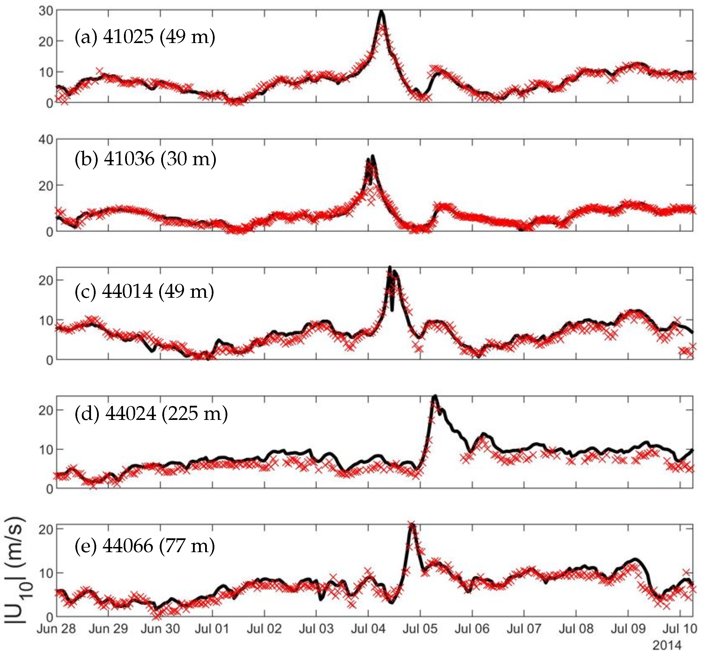
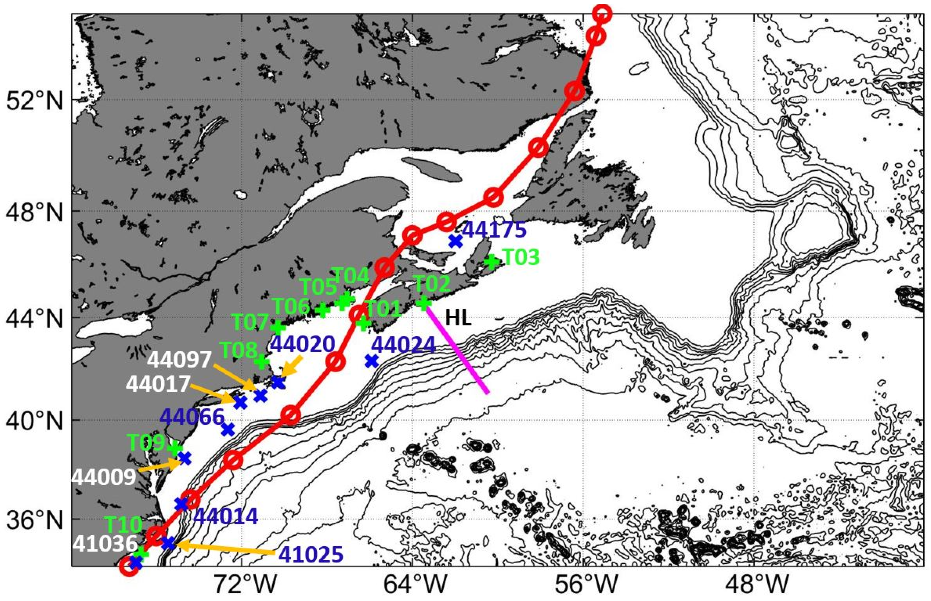
Since wind stress is an important driving force for CWMS-NWA, particularly during extreme weather conditions, we first examine the accuracy of blended winds during Hurricane Arthur. The blended wind speeds (Figure 2) and directions are compared with observations made at the National Data Buoy Center (NDBC) and ECCC buoys. The locations of these buoys are marked in Figure 1. Buoys 41025, 44024 and 44175 are all on the RHS of the storm, buoys 41036 and 44014 are along the storm track, and the rest (44009, 44017, 44020, 44066 and 44097) are on the left hand side (LHS) of the storm track. Buoys 41025 and 41036 are along the GuS while buoy 44024 is under the influence of tidal currents in the GoM.

As shown in Figure 2, the observed wind speeds are well represented by the blended winds during Hurricane Arthur at five buoys (41025, 41036, 44014, 44024 and 44066). At buoy 41025, for example, the blended winds agree very well the observations with only minor discrepancies (overestimated by up to ∼4 m/s) on 28 June and (overestimated by up to ∼5 m/s) 4 July (Figure 2a). The blended wind speeds at buoy 41036 (Figure 2b) also agree with the observations except for noticeable differences on 4 July. At buoy 44014 (Figure 2c), the blended winds are also in general agreement with observations except some over/underestimations. The blended winds at buoy 44024 (Figure 2d) reproduces well the temporal variations for the observed winds with slight overestimation at the low winds. Finally, the blended winds at buoy 44066 (Figure 2e) match the observed winds apart from some minor differences during a few of the fluctuations of the wind speed.

The performance of the blended winds in presenting the observed wind speeds at each buoy is quantified using five error metrics (Appendix A and

Table 2. Error statistics for the speeds of Moody’s HWind (m/s) at seven buoys within the simulated period.

Station	R (%)	RMSE (m/s)	${\mathit{\gamma }}^2$	RB (m/s)	SI
41025	96.5	1.11	0.08	0.02	0.16
41036	95.2	1.35	0.11	0.03	0.20
44014	91.9	1.49	0.17	0.09	0.24
44020	90.2	1.35	0.19	−0.02	0.18
44024	95.4	2.02	0.12	0.26	0.31
44066	93.5	1.30	0.13	0.09	0.19
44175	83.4	3.46	0.48	0.55	0.68
Average	92.3	1.73	0.18	0.15	0.28

). Note that observational wind data at buoys 44009, 44017 and 44097 are not available for the study period.

At buoy 41025 located just west of Hatteras canyon and offshore of North Carolina, the blended wind speeds represent very well the observational wind speed data (Figure 2a) with R ≈ 96.5%, RMSE ≈ 1.11 m/s, ${\gamma }^2$ ≈ 0.08, RB ≈ 2 cm/s and SI ≈ 0.16. Buoy 41036 is near the southern boundary of the model domain and has error metrics highly similar to buoy 41025; with R ≈ 95.2%, RMSE ≈ 1.35 m/s, ${\gamma }^2$ ≈ 0.11, RB ≈ 3 cm/s and SI ≈ 0.20. The observational wind speeds at buoy 41036 suggest that the eye of Arthur passed over the buoy at about 12:00:00 4 July. While the eye does appear in the blended wind speeds, it is far less pronounced and thus the wind speeds are overestimated (Figure 2b). Buoy 44014, which is 64 nautical miles (∼119 km) east of Virginia Beach also has particularly good error metrics: R ≈ 91.9%, RMSE ≈ 1.49 m/s, ${\gamma }^2$ ≈ 0.17, RB ≈ 9 cm/s and SI ≈ 0.24. Over the study period, some differences between the blended and observed wind speeds at buoy 44014 are due mainly to the overestimation by Moody’s HWind during 3–5 July (Figure 2c). The statistical errors at buoy 44020 situated in Nantucket Sound are very similar to the other buoys discussed above. The relatively large errors of the blended wind speeds at buoy 44024 in Northeast Channel come from the small but systemic overestimations of the observed wind speeds at this buoy (Figure 2d). With minor discrepancies, the blended wind speeds at buoy 44066, located at about 139 km to the east of Long Beach, New Jersey, resemble the buoy wind speed data (Figure 2e). The error metrics for the blended winds at buoy 44066 are very comparable to the average of the seven buoys. Buoy 44175 is near the Madeleine Islands in the Gulf of St. Lawrence (GSL). The error metrics at this buoy (R ≈ 83.4%, RMSE ≈ 3.46 m/s, RB ≈ 55 cm/s, SI ≈ 0.41 and ${\gamma }^2$ ≈ 0.48) are all noticeably worse than the average of the seven buoys. Note that by the time that Arthur reaches buoy 44175, it is an extra-tropical cyclone. Moody’s HWind does not cover Arthur at this intensity.

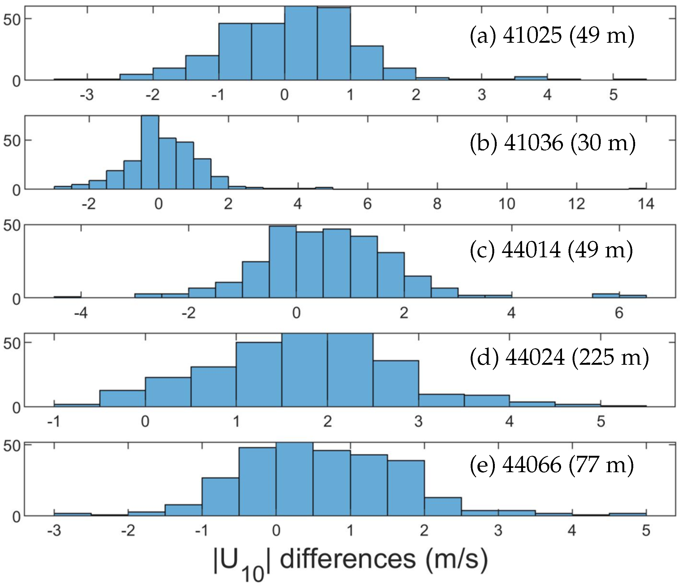
Differences between the blended wind speeds and buoy data are presented in histograms (Figure 3). At these five buoys, most of the differences in the wind speed are within ±2 m/s. At buoy 41025 near Diamond Shoals, NC, the maximum wind speed difference is ∼5 m/s (Figure 3a). While nearly all of the differences in the wind speeds are confined to ±5 m/s at buoy 41036, there is an outlier of ∼13.5 m/s (Figure 3b). Note that both the blended wind and buoy data show the eye of the hurricane passing over this location. The large difference of ∼13.5 m/s occurs on 02:00:00 July 4 where the blended wind speed is ∼32.6 m/s. At 02:00:00 July 4, the temporally-interpolated wind speed data is ∼19.1 m/s. However, the data at buoy 41036 is recorded as 14.9 m/s at 01:50:00 July 4 and 27.4 m/s at 02:20:00 July 4. This very large discrepancy appears to be a result of limits in the temporal output of the data and simple linear interpolation. By contrast, the histograms for the wind speed differences at buoys 44014, 44024 and 44066 are similar (Figure 3c, d and e respectively). The differences at these three buoys show a slightly positive skew, especially at buoy 44024.

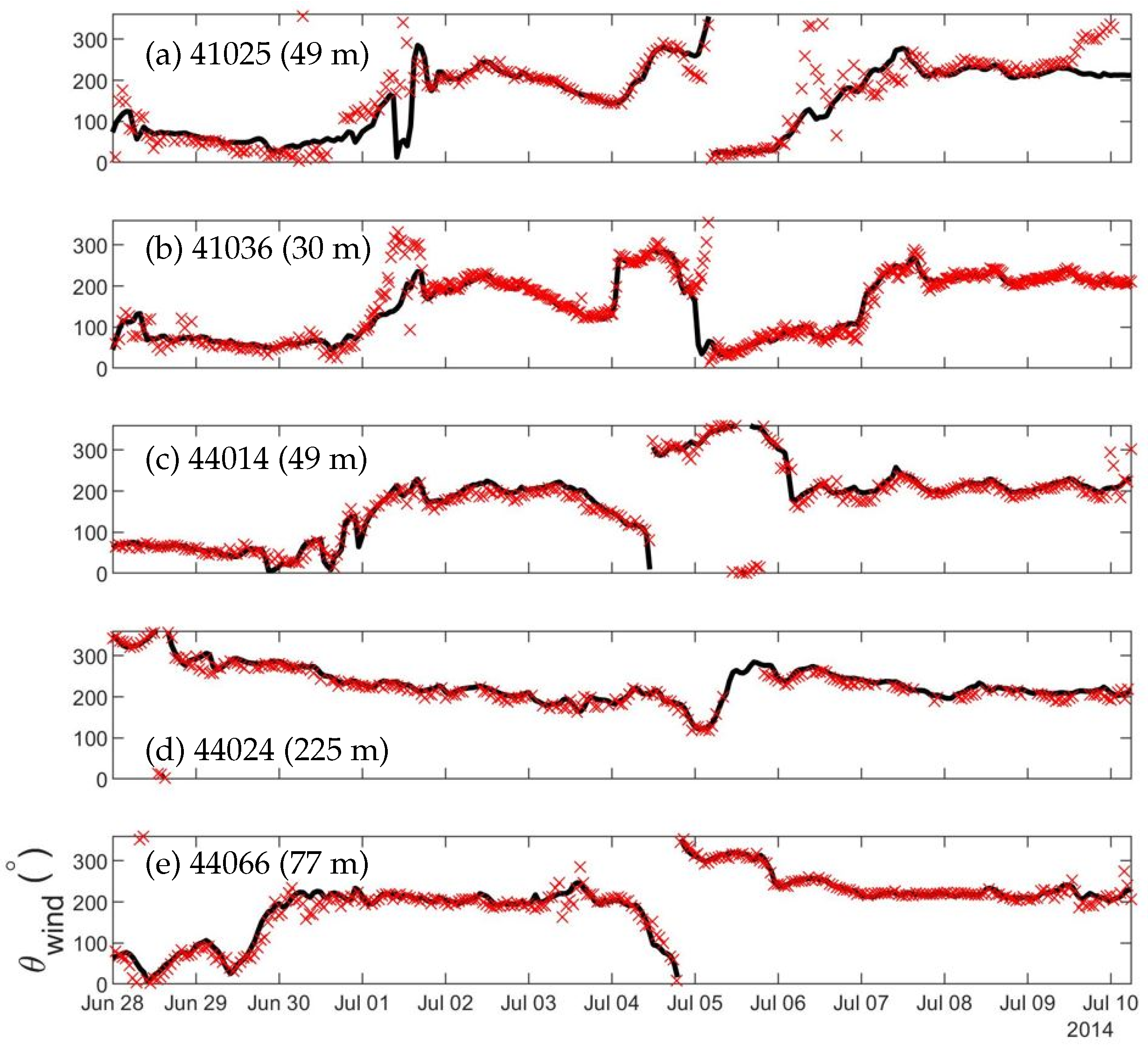
The observed wind directions are also generally captured well by the blended wind directions, but with relatively larger discrepancies than the wind speeds (Figure 4). At buoy 41025, for example, the blended wind directions agree very well with the observations during the study period, except for relatively large differences in wind direction on 1, 6 and 9 July. Some of the virtually large outliers such as on 30 June at buoy 41025 are due to the plotting style with the vertical axis being the 0–360 degree scale (Figure 4a). At buoy 41036, the large observed wind directional changes are not fully captured by Moody’s HWind on 1 July and at the beginning of 5 July (Figure 4b). The moderate changes in the observed wind directions at buoy 44014 are also not captured by the blended winds on 10 July (Figure 4c). At buoy 44024, differences between the blended wind directions and observed data are small (Figure 4d).

The blended wind directions at 41025 are in good agreement with observations, with R ≈ 84.6%, RMSE ≈ 51.0°, ${\gamma }^2$ ≈ 0.29, RB ≈ −0.07° and SI ≈ 0.31. The errors for the Moody’s HWind directions are smaller at buoy 41036 with R ≈ 91.1%, RMSE ≈ 33.2°, ${\gamma }^2$ ≈ 0.17, RB ≈ −0.03° and SI ≈ 0.21. Most of the observed wind directions are captured by the blended winds, but large discrepancies during a few short periods make up most of the RMSE (Figure 4b). The errors in the blended wind directions at buoy 44014 are highly similar to those at buoy 41025 (

Table 3. Error statistics for the wind directions (°) at seven buoys within the simulated period.

Station Name	R (%)	RMSE (°)	${\mathit{\gamma }}^2$	RB (°)	SI
41025	84.6	51.0	0.29	−0.07	0.31
41036	91.1	33.2	0.17	−0.03	0.21
44014	86.4	45.4	0.29	0.06	0.27
44020	54.5	49.5	0.95	0.02	0.23
44024	90.3	22.4	0.19	0.04	0.11
44066	92.0	28.1	0.16	0.01	0.14
44175	59.0	31.6	1.27	0.04	0.15
Average	79.7	37.3	0.47	0.008	0.20

). By contrast, the errors in the Moody’s HWind directions are relatively small at buoy 44024, with comparable R, ${\gamma }^2$ and RB values to buoy 41036. The RMSE and SI at buoy 44024 are both significantly smaller than the corresponding values at buoy 41036. The blended wind directions at buoy 44066 also have small errors that are consistently smaller than the average of the errors at the selected seven buoys. The ERA5-only winds at buoy 44175 reproduced the observed wind directions over the study period reasonably well.

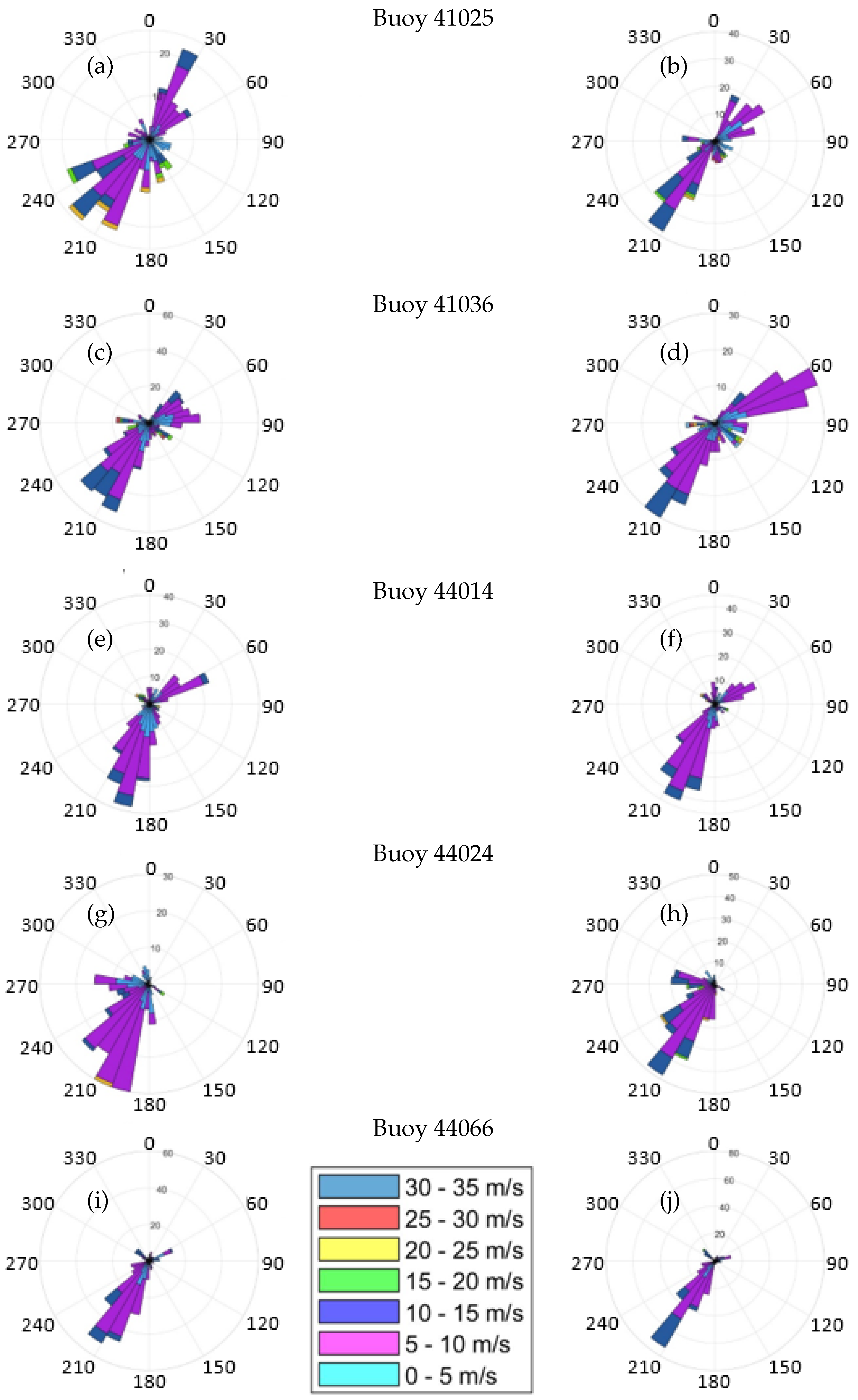
The observed wind speed and directional data and the wind speeds and directions from the blended winds at the five buoys are also displayed in wind roses in Figure 5. The wind rose for the data at buoy 41025 (Figure 5a) has a similar distribution to the wind rose for the blended wind at the buoy 41025 location (Figure 5b). Both the buoy data and blended winds are predominantly southwesterly with significant northeasterly winds as well. The blended winds are more southwesterly than the buoy data. At buoy 41036, the wind rose of the buoy data (Figure 5c) is also primarily southwesterly with an easterly to slightly northeasterly secondary component. There are fewer southwesterly components and more northeasterly components in the blended wind at 41036 (Figure 5d). Both the buoy data (Figure 5e) and blended winds (Figure 5f) are mostly slightly southwesterly with a secondary northeasterly component at buoy 44014. At buoy 44024, both the buoy data (Figure 5g) and blended winds (Figure 5h) are southwesterly with a smaller westerly component. The buoy data and blended winds at buoy location 44066 are both overwhelmingly southwesterly (Figure 5i and Figure 5j respectively).

3.2. Model Performance in Simulating Surface Waves

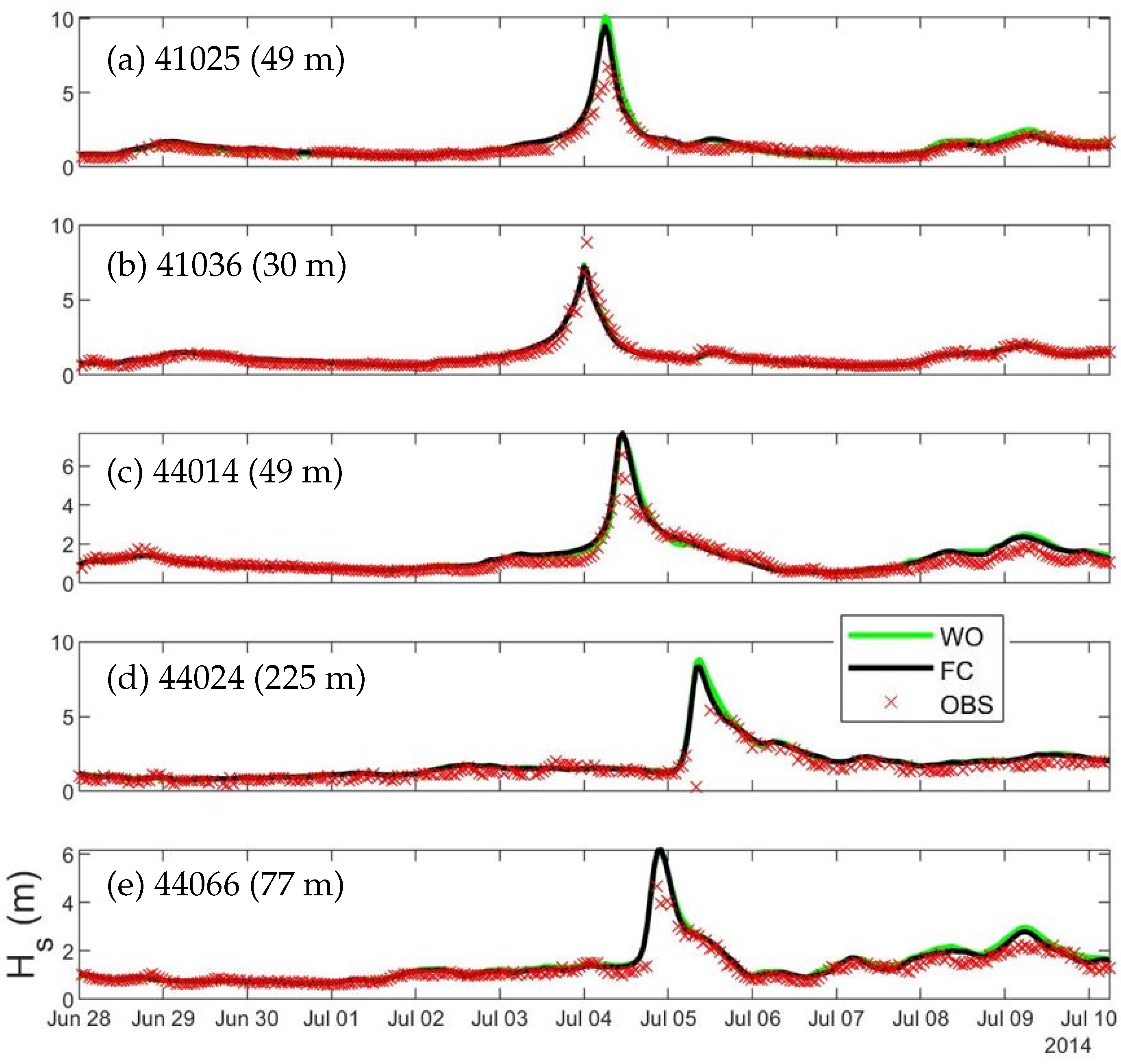
We next assess the performance of CWMS-NWA in simulating surface waves. The simulated SWHs are compared with wave observations at the NDBC and ECCC buoys within 150 km of the storm track over the model domain (Figure 6). At buoy 41025 on the RHS of the storm track, the SWHs in run FC generally agree with the observations. However, CWMS-NWA overestimates the maximum value of the observed SWHs ($H_s^{max}$) during the peak of the storm (Figure 6a). This overestimation of $H_s^{max}$ is due partly to the fact that the blended winds are higher than the observed winds (with differences up to ∼5 m/s) during the peak of the storm (Figure 2a). At buoy 41036, by comparison, the simulated $H_s^{max}$ is smaller than the observed value even though the blended winds are reasonable in comparison with the wind observations during the peak of the storm. Exact reasons for the large model deficiency at this buoy are unknown. Plausible reasons include model resolution, proximity of the southern boundary and observational errors. Relatively large model deficiencies in SWHs also occur during the peak of the storm at buoys 44014 (∼1.0 m or ∼15%), 44024 (∼1.0 m or ∼18%) and 44066 (∼1.1 m or ∼23%).

The simulated SWHs at buoy 44024 (on the RHS of the storm) are in good agreement with the observed SWHs except that the simulated $H_s^{max}$ is larger (up to ∼1.0 m) than the observation (Figure 6d). The lack of observational data at the peak of the storm at this buoy prevents us from calculating the actual model errors in simulating $H_s^{max}$. At buoy 44066 (LHS), there are also some missing observational surface wave data during the peak of the storm (Figure 6e).

To assess the performance of CWMS-NWA in simulating SWHs during the study period, three model error statistics (R, RMSE and ${\gamma }^2$) are calculated. At buoy 41036, which is located near the southern boundary of the model domain, the model performs reasonably well with R ≈ 88.8%, RMSE ≈ 19.7 cm and ${\gamma }^2$ ≈ 0.05. The model results in run FC underestimate the $H_s^{max}$ and lead the observed SWHs near the peak of the storm. These differences between the simulated and observed SWHs contribute to the large error metrics at buoy 41036 (Figure 6b). Buoy 44020 is located in the shallow water in Nantucket Sound. Model errors at this buoy likely result from the relatively coarse model resolution (1/12°) which is not able to capture all of the local dynamics over shallow coastal waters. Note that the surface wave observations at buoy 44024 were not available when Hurricane Arthur passed by the area of this buoy.

Differences in SWHs between model simulations (runs FC and WO) and the buoy data are shown in Figure 7. At buoy 41025 on the RHS, differences between the two model simulations and buoy data are similar for most of the storm time. However, when Arthur passes by, run FC has smaller differences with the data than run WO (Figure 7a). Both experiments overestimate the peak waves, although model results in run WO overestimate them more (by ∼0.6 m more than in run FC) and for a longer time period (∼7–8 h longer). At buoy 41036, the differences between the simulated SWHs in both runs and the buoy data are smaller, with underestimations of the maximum by ∼2 m (Figure 7b). Buoy 41036 is along the storm track and just north of the model southern boundary. Buoy 44014 is slightly to the left of the storm track. As with buoy 41025, both experiments overestimate the SWHs during the peak by over 2 m at buoy 44014 (Figure 7c). Here, run WO overestimates the peak SWH by ∼0.25 m more than run FC. Buoy 44024 is on the RHS of the storm track along the Northeast Channel and has large surface waves during the storm. Despite the buoy data missing at the peak, model results in both runs WO and FC overestimate the SWHs by over 2 m. The model errors in simulating $H_s$ are relatively larger in run WO than run FC just before and after the peak (Figure 7d). After the peak, run WO overestimates the SWHs by ∼0.28 m more than run FC. Buoy 44066 is on the LHS of the storm track in the MAB. Both runs WO and FC overestimate the SWHs by over 2 m along the peak (Figure 7e). However, in the 2–3 days leading up to the peak and the time after the peak, the differences between the model results in run WO and the buoy data are slightly larger than the differences between those in run FC and the buoy data, hence the larger RMSE (

Table 4. Error statistics for the significant wave heights (SWHs) (m) at ten buoys within the simulated period. Model results in fully coupled (FC) and Wave-Only (WO) experiments are used here.

Station	R (%)		RMSE (cm)		${\mathit{\gamma }}^2$
	FC	WO	FC	WO	FC	WO
41025	95.6	97.1	45.6	53.4	0.24	0.34
41036	88.8	89.0	19.7	17.2	0.05	0.04
44009	95.9	94.8	13.2	16.2	0.09	0.13
44014	95.8	94.8	37.1	39.6	0.17	0.19
44017	95.9	96.2	27.2	31.5	0.18	0.21
44020	82.7	84.4	21.3	21.7	0.32	0.29
44024	96.2	95.9	30.3	34.0	0.06	0.08
44066	96.2	96.6	22.7	28.1	0.20	0.21
44097	96.0	96.5	29.9	33.7	0.21	0.24
44175	97.1	97.4	28.4	26.1	0.11	0.11
Average	94.0	94.3	27.5	30.2	0.16	0.18

).

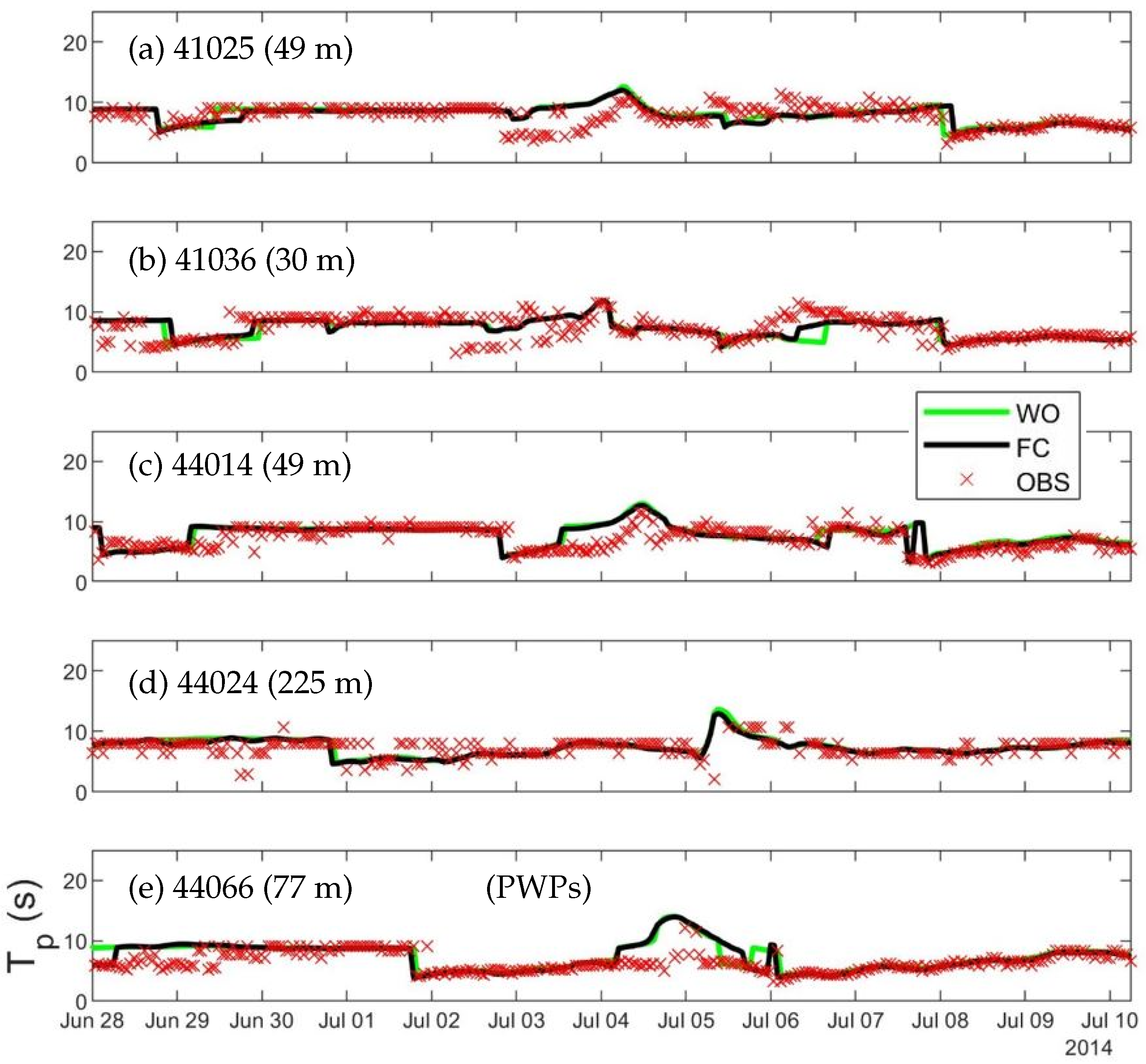
We next assess the model performance in simulating the surface wave periods by comparing the smoothed peak wave periods (PWPs) calculated from model results in run FC to observed PWPs at buoys 41025, 41036, 44014, 44024 and 44066 (Figure 8). The smoothed PWPs are calculated from the relative PWPs by applying a parabolic fit to the highest bin as well as two bins on both sides of the highest bin of the discrete wave spectrum [46]. The SWAN Team [46] recommends the smoothed PWP as a better estimate of the real PWP than the relative PWP. This is because the relative PWP “is related to the absolute maximum bin of the discrete wave spectrum and hence, might not be the ’real’ PWP” [46].

Examination of Figure 6 and Figure 8 suggests that the agreement between the simulated and observed PWPs is reasonable (average R ≈ 53.1%, average ${\gamma }^2\approx$ 1.43), but not as good as the agreement for the simulated and observed SWHs (average R ≈ 94.0%, average ${\gamma }^2\approx$ 0.16). For example, CWMS-NWA in run FC reproduces reasonably well most of the observed PWP time series at buoy 41025 with the typical values of PWPs about 5–9 s (Figure 8a). The only noticeable discrepancies occur on 3–4 July before the maximum value of PWP. The model results capture the general trends of the observed PWPs at buoy 41036 (Figure 8b) as well, with the simulated and observed results of about 5–10 s. Noticeable differences occur at this buoy with plausible reasons being the coarse model resolution and the limited discretization of the wave spectra (more detail at the end of the section). The agreement between the PWPs from the model results and the observations at buoy 44014 (Figure 8c) are similar to buoy 41025 with the relatively large discrepancies before the storm peak and small discrepancies at other times of the study period. CWMS-NWA also reproduces reasonably well the general pattern of the observed PWPs at buoy 44024, but the observed PWPs have more small-scale fluctuations than model results (Figure 8d). Finally, the model results at buoy 44066 match the observational PWPs, but the peak of the storm lasts much longer in CWMS-NWA (Figure 8e).

As shown in Figure 8, CWMS-NWA has deficiency in representing high-frequency variations of the observed PWPs. Different from SWHs, the PWPs are not based on the integral of the entire wave spectrum. The PWP is the inverse of the peak frequency ($f_p$), the frequency corresponding to the maximum wave spectral density. Capturing the peak wave spectral changes is thus more difficult than the full spectral SWHs, especially with limited discretized wave frequencies. The model relatively coarse resolution used in this study also limits how well the model reproduces the local topography, which also influences the surface waves. Despite these model deficiencies, CWMS-NWA has satisfactory skills in simulating the PWPs at these buoys (

Table 5. Error statistics for the smoothed peak wave period (PWP) (s) at ten buoys within the simulated period for model results in runs FC and WO.

Station	R (%)		RMSE (s)		${\mathit{\gamma }}^2$
	FC	WO	FC	WO	FC	WO
41025	40.0	47.6	1.7	1.6	1.07	0.95
41036	54.8	47.0	1.6	1.8	0.76	0.92
44009	64.9	68.7	1.7	1.7	1.01	0.89
44014	59.4	55.9	1.6	1.7	0.86	0.90
44017	73.0	75.7	1.5	1.5	0.60	0.52
44020	37.4	45.2	3.0	3.3	4.42	4.85
44024	52.7	53.6	1.2	1.2	0.87	0.88
44066	63.1	63.4	1.9	1.9	1.38	1.22
44097	67.0	71.9	1.6	1.5	0.91	0.74
44175	19.5	16.6	1.5	1.6	2.37	2.67
Average	53.2	54.6	1.7	1.8	1.43	1.45

). The PWP error metrics in this study are comparable to those in Lin et al. [18] with a few exceptions. Buoys 41025 and 41036 are both located near the southern boundary of the model domain. Thus, any errors in the boundary conditions could propagate through the model output at both buoys. Buoy 44175 is situated in the GSL between Prince Edward Island and the Madeleine Island. Only the coarse-resolution background ERA5 winds are available over the GSL. SWHs and PWPs are also limited at buoy 44175 by the reduced fetch and local topography.

3.3. Model Performance in Simulating Surface Elevations

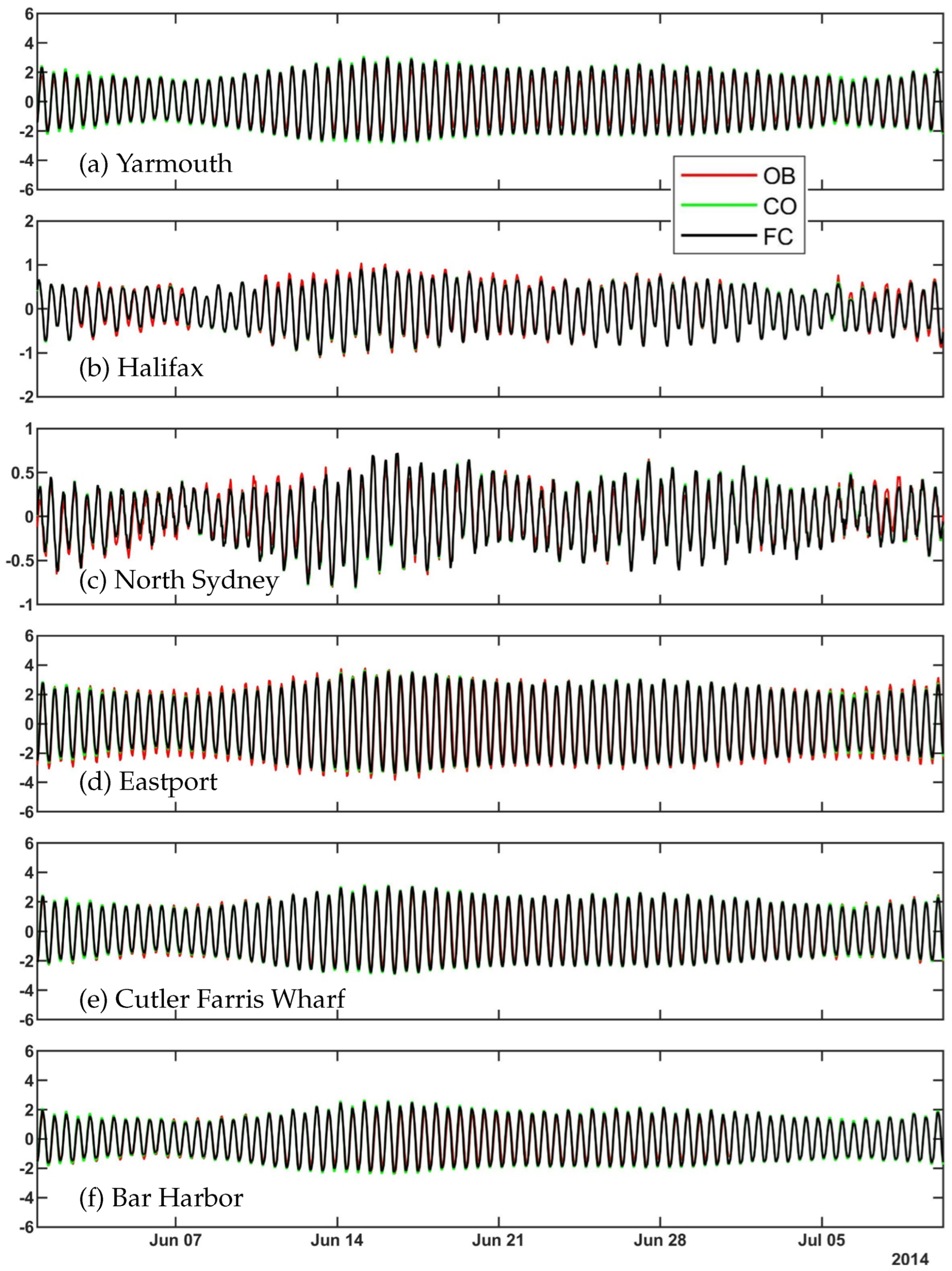
The simulated surface elevations in run FC are compared with in-situ measurements at ten tidal gauge stations whose locations are shown in Figure 1. The observed and simulated total surface elevations at six of these stations are shown in Figure 9, from the beginning of June to the end of the Hurricane Arthur storm period on 10 July. The tidal gauge observations at Saint John, NB are excluded due to some issues with data quality in 2014. The observed total surface elevations at Yarmouth, Eastport, Cutler Farris Wharf and Bar Harbor all have large oscillations associated with large tides in the inner GoM and BoF. Large tidal elevations also occur at Halifax and North Sydney, but the tides are weaker over the Scotian Shelf (ScS) than the GoM and BoF.

There is a good agreement between the simulated and observed total surface elevations at ten tidal gauge stations listed in

Table 6. Error statistics in simulating the total surface elevations at ten tidal stations within the study period of 1 June–10 July 2014 for model results in runs FC and CO.

Station	R (%)		RMSE (cm)		${\mathit{\gamma }}^2$
	FC	CO	FC	CO	FC	CO
Yarmouth (T01)	99.1	98.8	33.3	39.8	0.07	0.11
Halifax (T02)	98.7	98.7	8.0	8.1	0.03	0.03
North Sydney (T03)	97.1	97.2	7.1	7.2	0.06	0.06
Eastport (T04)	97.2	95.8	46.2	56.2	0.06	0.08
Cutler Farris Wharf (T05)	98.5	97.6	27.8	37.0	0.03	0.06
Bar Harbor (T06)	97.8	96.5	28.5	37.4	0.06	0.10
Portland (T07)	96.5	94.7	30.0	39.1	0.09	0.15
Boston (T08)	96.0	94.1	31.6	40.5	0.10	0.16
Cape May (T09)	96.5	96.5	16.6	16.2	0.10	0.09
Duck (T10)	95.8	95.7	10.7	10.7	0.08	0.08
Average	97.3	96.6	24.0	29.2	0.07	0.09

. The error metrics for the simulated total surface elevation at Yarmouth are: R ≈ 99.1%, RMSE ≈ 33.3 cm and ${\gamma }^2$ ≈ 0.07. The relatively large R value and ${\gamma }^2$ value at Yarmouth suggest that the CWMS-NWA is able to reproduce the large observed tides exceptionally well at this location. Model results of the total surface elevations have high R and low errors at four locations in the GoM: Eastport, Cutler Farris Wharf, Portland and Boston with R at 96% or higher. The RMSEs at these four stations are about 46.2 cm at Eastport and about 27.8, 28.5 30.0 and 31.6 cm respectively at Cutler Farris Wharf, Bar Harbor, Portland and Boston. The simulated results of the total surface elevations at these GoM tidal stations all have very small ${\gamma }^2$ values as well. Cutler Farris Wharf has the smallest ${\gamma }^2$ of the GoM tidal stations (≈ 0.03), followed by Eastport and Bar Harbor (≈ 0.06), Portland (≈ 0.09) and Boston (≈ 0.10).

Though some spatial variability occurs in the model errors of CWMS-NWA for simulating the total observed surface elevations, the consistent low values of model errors in the GoM demonstrate a very good simulation of the tidal oscillations. Along the coast of Nova Scotia, the simulated total surface elevation at Halifax and North Sydney have comparable R and ${\gamma }^2$ values to the GoM locations. However, the RMSEs are much smaller at Halifax (∼8.0 cm) and North Sydney (∼7.1 cm) than the values at the four GoM tidal gauges. The main reason for small RMSEs at Halifax and North Sydney is that tides are much weaker at Halifax and North Sydney than they are within the GoM. The RMSEs are smaller at Cape May, NJ and Duck, NC than the GoM locations, but the R and ${\gamma }^2$ values at the Mid-Atlantic Bight (MAB) locations are similar to the model results at Boston.

The observed and simulated surface elevations are further examined using the tidal analysis. Tidal harmonics are computed from both the observational data and the model results by the MATLAB T_TIDE package [47]. Thirty-five tidal constituents are identified from the 39-day time series of the total surface elevations for both the observational data and model output. From the identified tidal constituencies of the observed data, only the O1, K1, N2, M2, S2 and L2 have amplitudes greater than 0.09 m at any of the six tidal gauge stations. The simulated tidal surface elevations are in good agreement with the observed tidal elevations at the six tidal gauge stations. Tidal surface elevations largely resemble the total surface elevations at the six tidal gauge stations. The model errors in both the magnitudes and the phases of the tides could be due to the limited horizontal resolution of the model. The error metrics for the simulated tidal surface elevations are small.

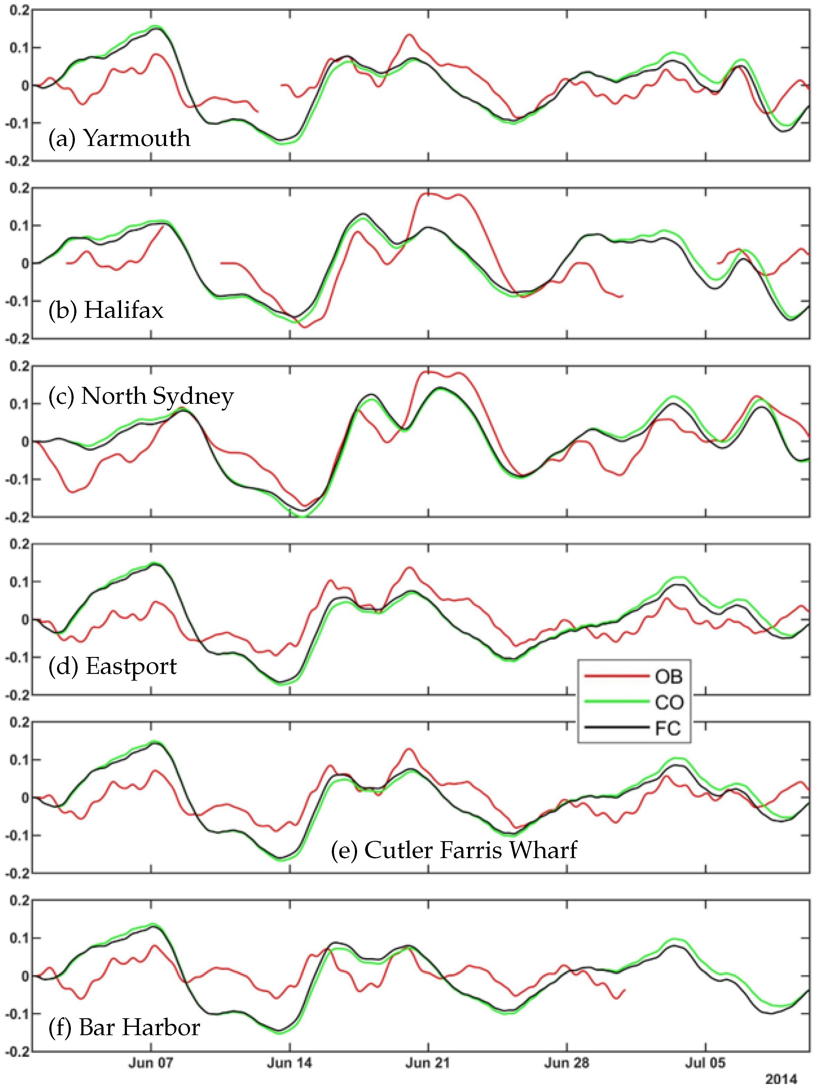
Tidal residuals of the surface elevations are calculated by subtracting the tidal elevations from the total surface elevations. To remove any tidal signals, the residuals are passed through a low pass filter with a cutoff frequency corresponding to a period of 13 h to remove high-frequency noise. The model output residuals and the residuals of the observed data are shown in Figure 10. The tidal residuals from the model results agree fairly well with those from the observed data. Slight differences between the residuals from run CO and run FC occur at all six stations plotted. These small differences suggest that WCIs have a minor role in modifying the residual surface elevations.

Zhang and Sheng [48] used a 2D barotropic ocean circulation model to examine extreme sea levels resulting from tides and storm surges over 32-year simulations over coastal waters of the NWA. The atmospheric and tidal forcing were used in their studies. They also decomposed the simulated and observed sea levels into tidal and non-tidal components. They examined hourly time series of both the tides and storm surges associated with hurricanes and winter storms. From their experiments, they found that the 2D model has satisfactory skills in simulating storm surge magnitudes. Yang et al. [49] used ROMS in barotropic mode to study interactions between tides and storm surge during Hurricanes Bill in 2009 and Dorian in 2019. Consistent with previous studies, they found relatively large non-linear tide-surge interactions, with maximum changes to the sea levels over the BoF, GSL and Northumberland Strait reaching 0.2 m, 0.4 m, and 0.3 m, respectively during Hurricane Dorian. They found that the non-linear bottom friction effect had a much larger contribution than the advection effect and the non-linear shallow water effect over coastal shelf waters. A more thorough analysis would be required here to investigate the non-linear tide-surge interactions during Hurricane Arthur. However, other studies used numerical models to investigate storm surge during Hurricane Arthur (as discussed later) [17,50,51].

3.4. Model Performance in Simulating Temperature and Salinity

We next assess the performance of CWMS-NWA in simulating temperature and salinity using satellite remote sensing data and in-situ hydrographic observations.

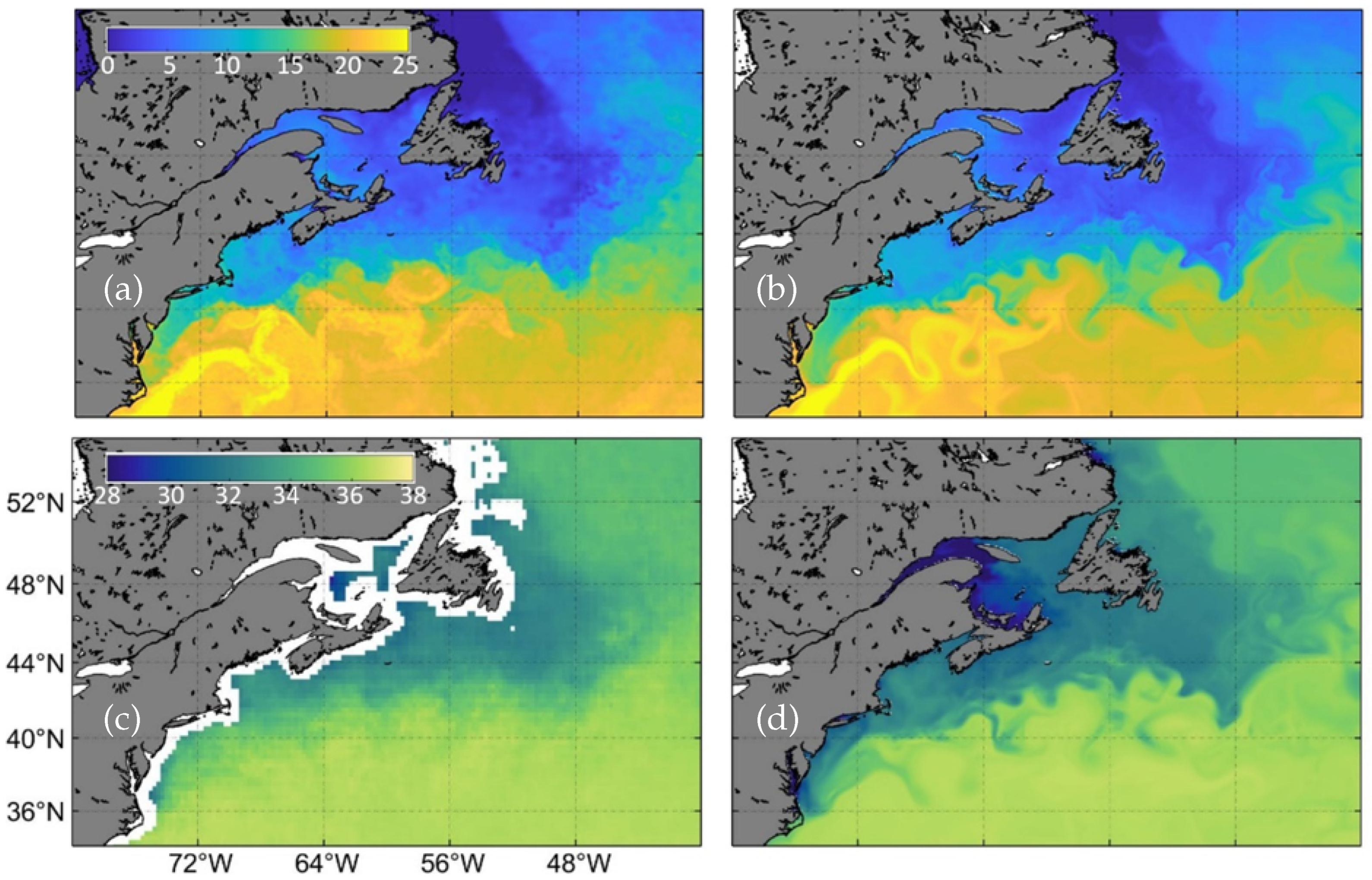
The simulated daily-mean sea surface temperature (SST) in run FC is first compared with the daily averaged SST from the European Space Agency (ESA) SST Climate Change Initiative (CCI) project [52] which is the Level-4 (L4) global SST product with a resolution of $\mathrm{0.05°}$ [53]. As shown in Figure 11 on 22 May 2014, CWMS-NWA reproduces reasonably well the observed large-scale temperature patterns such as warm SST carried by the GuS and the cold water carried by the Labrador current (LaC). Some of the cooler water on Georges Bank as well as the cooler water in the GSL are also reproduced by CWMS-NWA. It should be noted that without data assimilation, CWMS-NWA has limited skills in reproducing the observed locations, sizes and shapes of meanders and smaller scale features due mainly to highly nonlinear processes controlling evolution of meanders, filaments and smaller scale frontal structures associated with the GuS and LaC. Furthermore, the simulated GuS is located further to the north in comparison with observations. CWMS-NWA also reproduces two prominent coastal currents on the ScS: the Nova Scotia Current (NSC) [54] and the Shelfbreak Current (SbC) [55]. The horizontal resolution of CWMS-NWA is about 6 km on the ScS and GoM. Therefore, this modelling system has limited skills in generating small-scale features of circulation and hydrography.

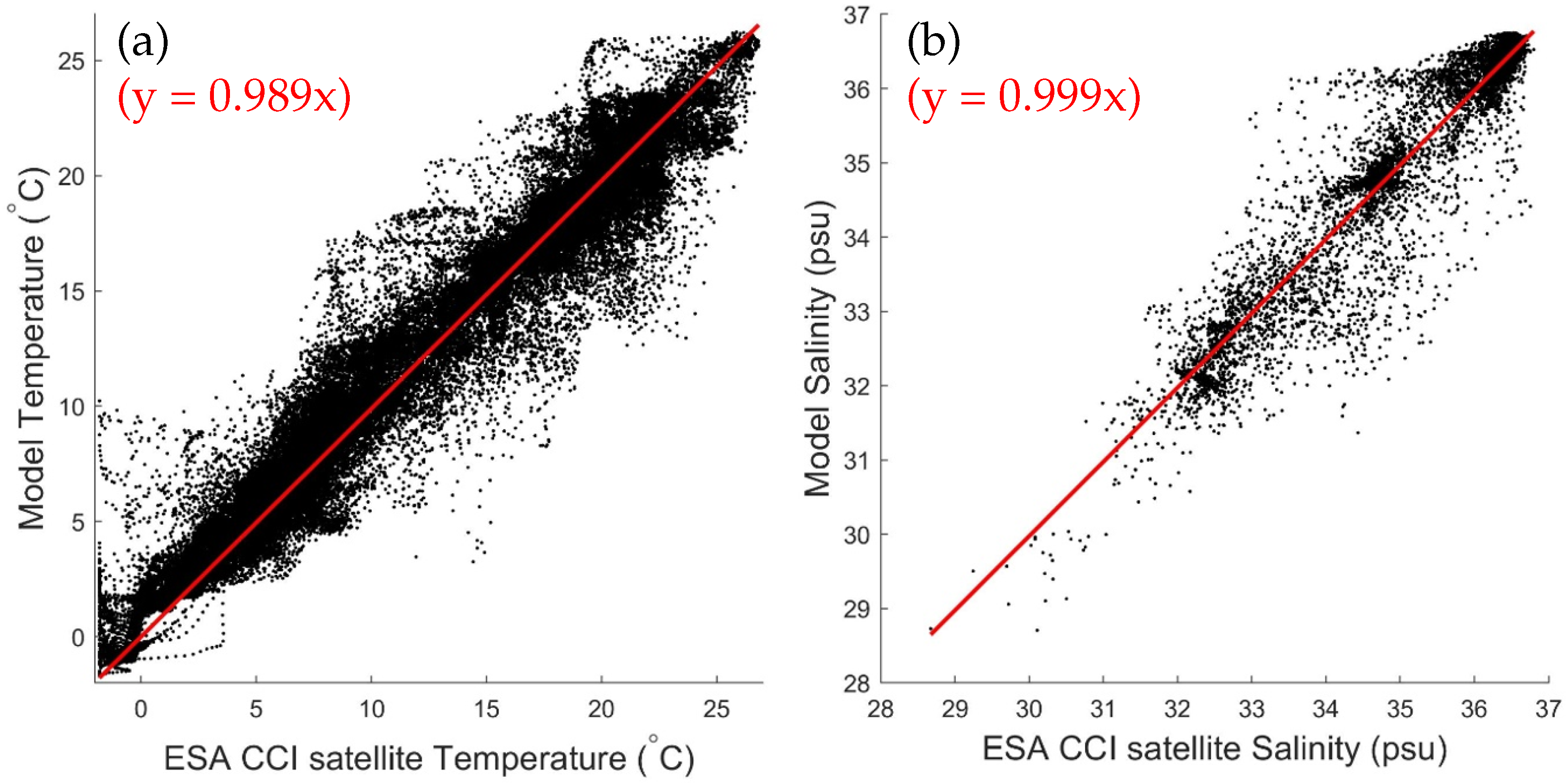
Figure 12a is a scatter plot of the SST between the ESA CCI satellite and model results with the R value of about 97.8%. The small bias demonstrated by the red line bisecting the scatter is confirmed by the small RB (∼8.6 × ${10}^{-3}$ °C). The comparatively large RMSE (∼1.6 °C) and SI (∼0.12) can be attributed to large model–biases for the small-scale features. For example, both the satellite SST data and model results show warm and cold core eddies, but with large differences in size, shape and position which result in large RMSE and SI. However, the small RB indicates that the simulated SST produced by CWMS-NWA is not systemically too warm or too cold on average over the entire model domain.

The simulated weekly average sea surface salinity (SSS) in run FC is also compared with ESA CCI satellite SSS data [56] (Figure 11). The ESA satellite SSS data calculated using a 7-day running mean for May 18–25 has a horizontal resolution of 1/4°. The satellite SSS data have relatively large errors over coastal regions. Thus, we cannot assess the model performance in simulating SSS over coastal waters near river mouths, where there are freshwater discharges to estuaries and the ocean. Both the satellite SSS data and the model results show that lower salinity water is confined to the shelves and shoreward of the shelves, with meanders and eddies from the higher salinity GuS present. To the south of the GuS, both the observed salinity data and results from run FC show relatively high SSS.

The weekly averaged SSS comparison between the ESA satellite data and model results is also examined in the scatter plot shown in Figure 12b. This SSS produced by CWMS-NWA has a relatively small RB with respect to the satellite data and a high R (∼$90.8\%$), with the RMSE ≈ 0.5 psu and SI ≈ $1.4\times {10}^{-2}$. The main reasons for large model deficiencies in simulating salinity (and temperature) include (a) less reliable air-sea fluxes and vertical mixing, (b) coarse horizontal resolution of CWMS-NWA and (c) the absence of data assimilation to reduce model errors arising from the initial conditions and the nonlinear nature of ocean circulation and vertical mixing.

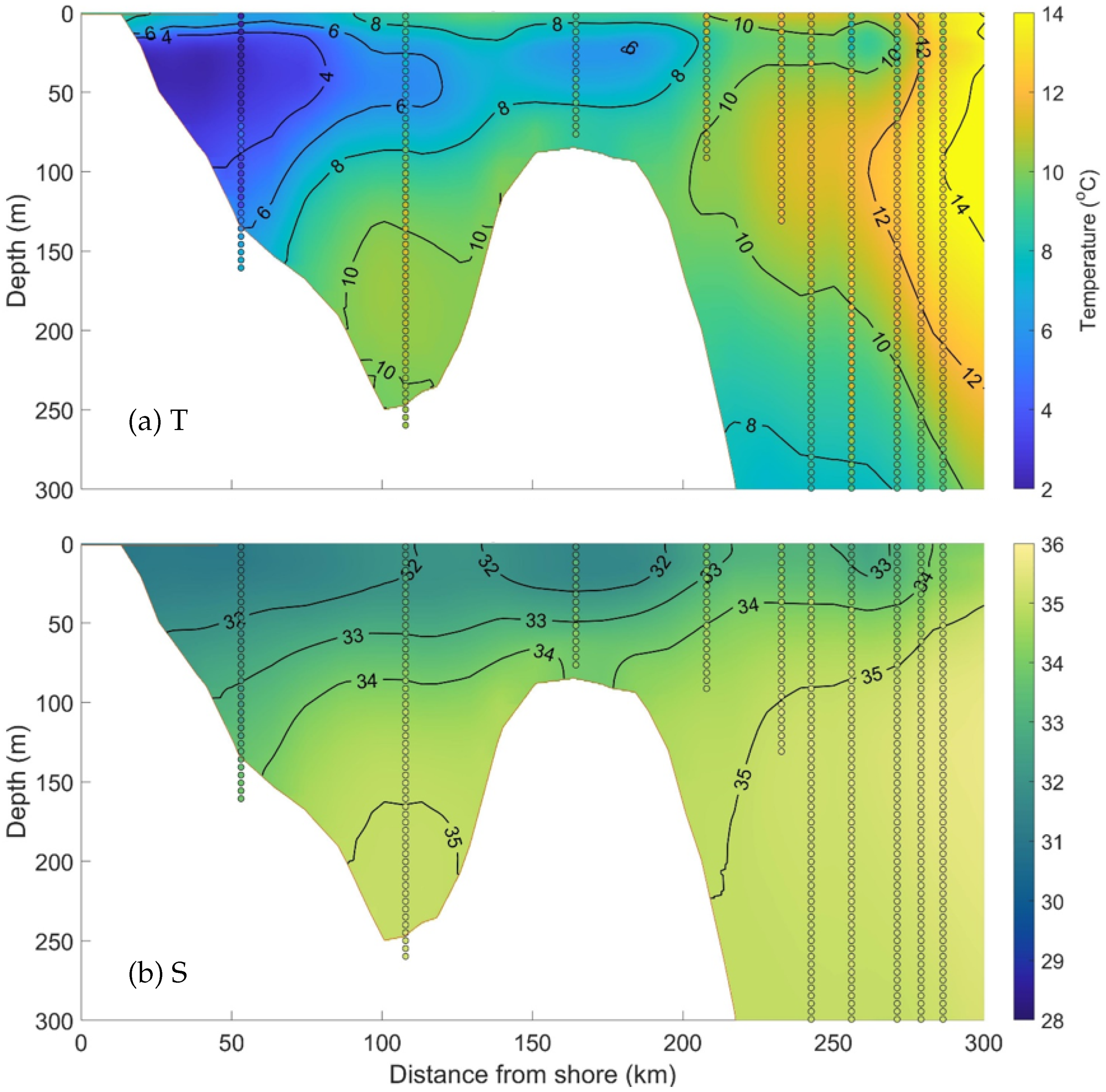
Vertical distributions of the model results in run FC are compared with in-situ hydrographic observations made by the Atlantic Zone Monitoring Program (AZMP). The AZMP temperature data along the Halifax Line (HL as marked in Figure 1) are shown in Figure 13a together with the two-day average (00:00:00 21 May 2014 to 00:00:00 23 May 2014) of the simulated temperature in run FC. Both the observed and simulated temperature along the Halifax line show the cold water near the coast associated with the coastal cold water mass transported by the NSC from the eastern ScS to the southwestern ScS. A second cold water mass near the shelf break indicates the presence of the SbC which carries the relatively cold water mass from the eastern ScS to the shelf break of the southwestern ScS. Offshore from the slope, the warmer temperature signifies the presence of Warm Slope Water (WSW). The Slope Water is a mixture of warm GuS water with colder water from the SbC and consists of two parts: the aforementioned WSW and Labrador Slope Water (LSW) [55,57,58,59]. Examination of observed and simulated temperatures shown in Figure 13a suggests the reasonable skills of CWMS-NWA in simulating the vertical distributions of temperature over the ScS.

Vertical distributions of simulated and observed (AZMP) salinity along the Halifax line are shown in Figure 13b. The simulated salinity in the upper layer near the coast and over the shelf break is significantly lower than the salinity at greater depths and offshore. These lower salinities show the presence of the NSC and the SbC respectively. Lower salinity water near the surface and further offshore indicates the flow of water from the GSL in the upper ∼50 m of the Halifax line. The saltier water seaward of the shelf break indicates the presence of the previously described WSW. The tilted haloclines suggest that there is a shoreward flow of the WSW from ∼50–200 m where some of it spills over the shelf break and into Emerald Basin. Figure 13b demonstrates general agreement between the AZMP salinity data and simulated salinity along Halifax line. It should be noted that, at around 50 km from the shore, the salinity in run FC at depths greater than ∼110 m is saltier than the observed salinity data. The simulated salinity is fresher near the surface at the ∼110 km, ∼170 km and ∼210 km water columns. Exact reasons for model deficiency in simulating salinity and temperature along transect of the Halifax line are not known. Plausible reasons include the coarse model resolution, inaccurate vertical mixing and insufficient air-sea fluxes.

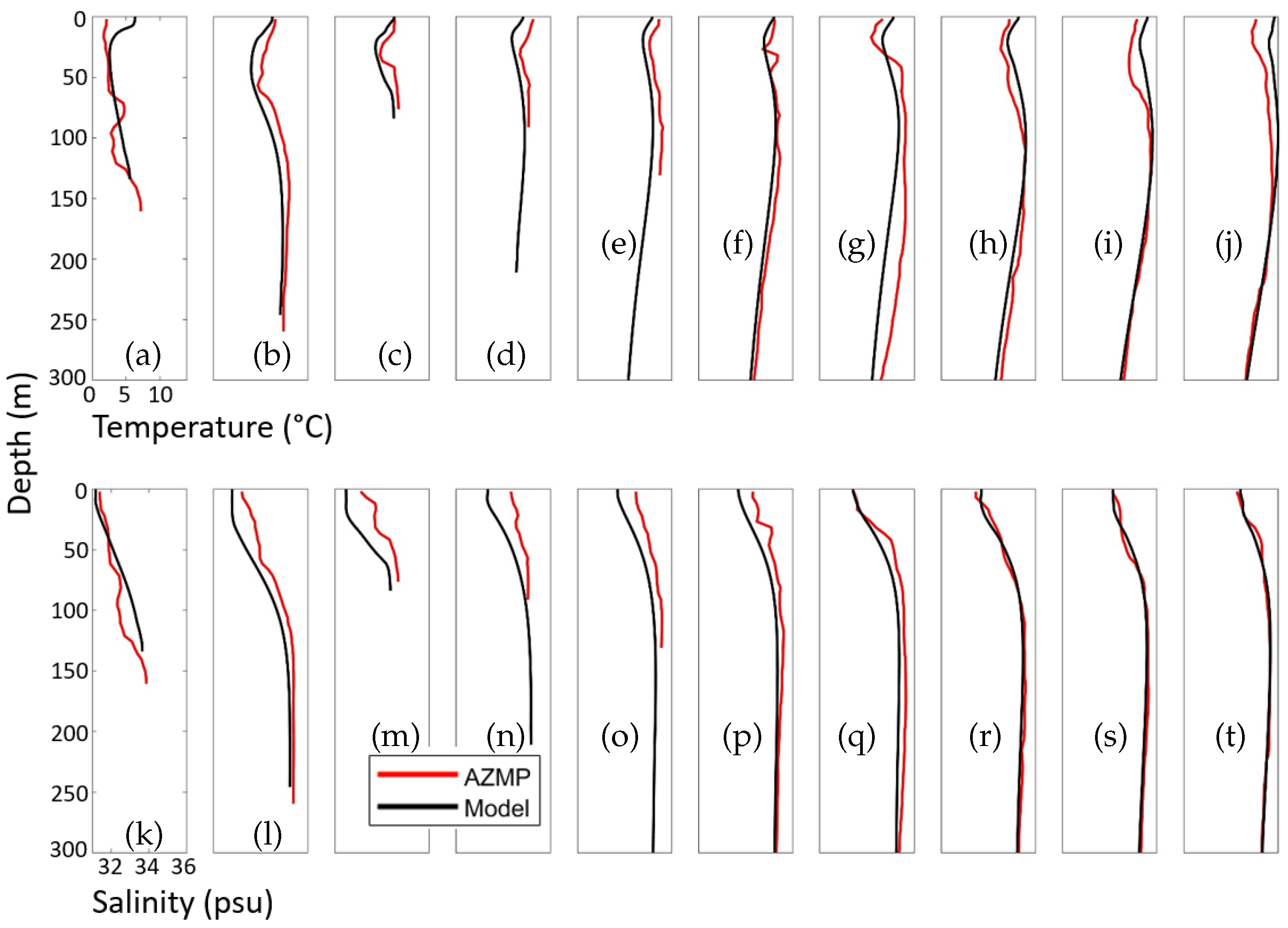
The ten vertical profiles of the observed temperature and salinity data from AZMP are compared with interpolated model results along Halifax line (Figure 14). For the two-day average of the simulated temperature on 22 May at the 10 vertical profiles, the RB is small (∼−3.5 × ${10}^{-2}$ °C) while the RMSE (∼1.2 °C) and SI (∼0.11) are relatively large but still acceptable. In particular, CWMS-NWA reproduces very well the AZMP temperature data towards the middle temperature range with more bias at higher and lower temperatures, especially at the surface (Figure 14a). Note that there are limits on the amount of data available. For example, the model results include both the NSC and SbC, but it cannot resolve all of the detailed local circulation. The relatively coarse 1/12° horizontal resolution also produces some discrepancy with the bathymetry which in turn affects the local dynamics.

Examination of ten vertical profiles of the observed (AZMP) and simulated salinity along the Halifax line (Figure 14b) shows that most of the variability of the salinity is near the surface. Salinity for most of the water at depths deeper than 200 m is confined to a narrow range of salinity (∼34.9–35.6 psu), with a small degree of scatter. Overall for the model performance in generating the vertical distribution of salinity along the Halifax line, the RB (∼−6.8$\times {10}^{-3}$ psu) and SI (∼0.01) are both small and the RMSE (∼0.42 psu) is also reasonable.

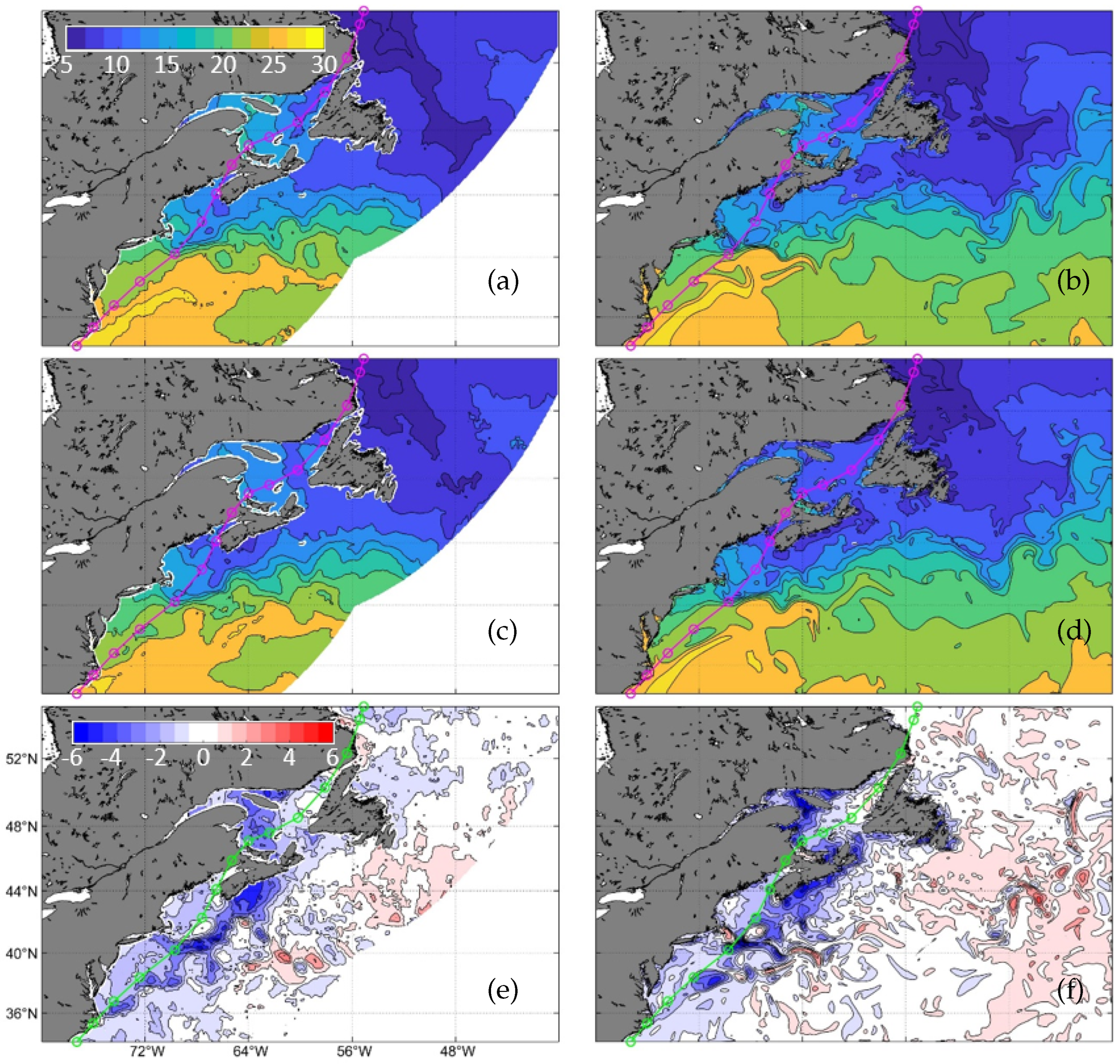
The international MAXSS (Marine Atmospheric eXtreme Satellite Synergy) Project funded by the ESA has an archive of analyzed satellite data for major storms from 2009–2020 (https://data-maxss.ifremer.fr/added_value/storm-wake/) [60] e.g., (accessed on 1 March 2023). These satellite remote sensing data include the SST as well as changes in the SST due to Hurricane Arthur. The pre-storm SST (SST^pre) and post-storm SST (SST^post) as well as the difference (${\Delta }^{st}$SST = SST^post− SST^pre) between the MAXSS SST data and CWMS-NWA results are shown in Figure 15. Here, SST^pre denotes the pre-storm SST averaged between 06:00:00 30 June 2014 and 06:00:00 5 July 2014. SST^post denotes the post-storm SST averaged between 06:00:00 5 July 2014 and 06:00:00 10 July 2014.

The warm waters carried by the GuS are visible in both the observed and simulated fields of SST^pre and SST^post (Figure 15a–d). Over the southwest part of the model domain and off the coast of North Carolina, the high SST in both the MAXSS observations and model results suggest the intense northeastward jet as part of the GuS. Large differences occur however in the simulated and observed positions of a large-size meander. The meander is close to the storm track and centered at ∼70° W, ∼38° N in the simulated SST^pre (Figure 15b), but is further to the southeast and centered at ∼68° W, ∼37° N in the MAXSS observations (Figure 15a). Large differences between the observed and simulated SST also occur with other small-scale features such as eddies separating the warmer water from cooler SST. These small-scale eddies are shaped differently and located in different positions in the model results than the MAXSS observations. These differences in the eddies and meanders in the SST^pre are due to the highly nonlinear nature of the ocean circulation. Pathways of the LaC are also visible in both the simulated and observed SST^pre. The LaC includes a cold SST at the northern boundary of the model domain along the coast of Labrador. This cold water is transported to the southeast along the shelf edge towards Flemish Cap. Multiple bifurcations of the LaC are visible to the east of Newfoundland in the MAXSS SST^pre data. One branch heads to the east and a second smaller and branch turns southwest along the coast of southeastern Newfoundland. The second bifurcation occurs to the east of the first bifurcation. At the second bifurcation, the main branch of the LaC continues eastward, while the rest of the cold water flows southward through Flemish Pass. Both the model results and MAXSS SST^pre show relatively warm water in the GSL. In the GoM and ScS relatively mild SST^pre occurs with slightly different cool anomalies such as the colder water along Georges Bank. CWMS-NWA reproduces the general distribution of the observed post-storm SST over the NWA (Figure 15c,d), with relatively warm waters carried by the GuS and relatively cold waters carried by the LaC. Large differences however occur between the observed and simulated post-storm SST.

Noticeable differences occur in the observed and simulated locations and shapes of small-scale features in SST^post. SST^post is cooler along the RHS of the storm track than SST^pre for both the MAXSS SST data and the model results. Along the Grand Banks and Flemish Cap, the cold water from the LaC bifurcations is warmer than the SST^pre for both MAXSS and CWMS-NWA.

Examination of observed and simulated storm-induced changes of SST (Figure 15e,f) shows that CWMS-NWA has skills in simulating the storm-induced cold wake, especially to the right of the storm track, and warm anomalies over Georges Bank and the southwest tip of Nova Scotia. The stronger storm-induced cooling ∼−4 to −6 °C covers a broader area of Georges Bank in the MAXSS SST data than in CWMS-NWA. Conversely, the SST cooling in the GSL near Anticosti Island is more intense in the model results (∼6 °C) than the observations (∼3 °C). CWMS-NWA does not reproduce the ∼1 °C cooling to the north of Newfoundland and along the coast of Labrador. The simulated ${\Delta }^{st}$SST is also smaller than the observed storm-induced cooling on the LHS of the storm track in the MAB and GoM. Both the satellite and simulated ${\Delta }^{st}$SST also have warming (∼1–2 °C) to the east of the cold wake. The observed storm-induced warm pattern between 56 and 64° W and ∼38 and 40° N is not in the simulated ${\Delta }^{st}$SST. Instead, the simulated storm-induced warming is more dispersed than the satellite observations.

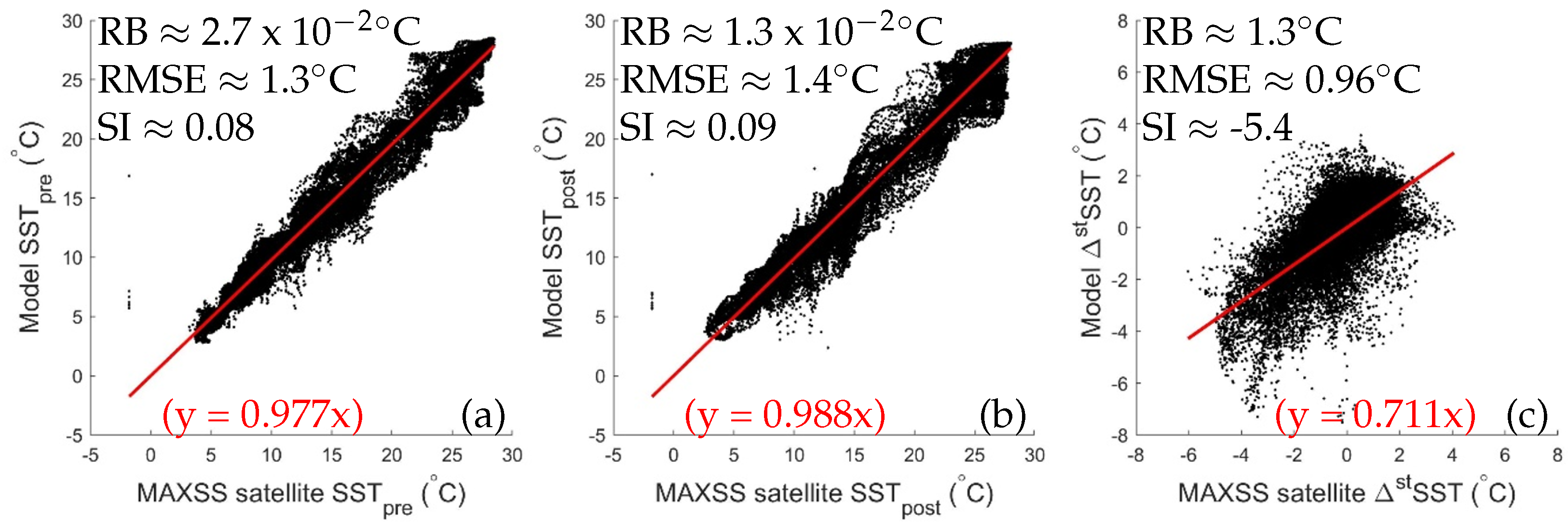
Comparisons of the SST^pre, SST^post and ${\Delta }^{st}$SST between satellite data and simulated results are further examined in the scatter plots shown in Figure 16a, b and c respectively. Both the simulated SST^pre and SST^post have small RBs (∼2.7 $\times {10}^{-2}$ °C and ∼1.3 $\times {10}^{-2}$ °C respectively) and SIs (∼0.08 and ∼0.09 respectively). The RMSEs of SST^pre and SST^post are not large either (∼1.3 °C and ∼1.4 °C respectively). By contrast, ${\Delta }^{st}$SST has a larger RB (∼1.3 °C) and SI (∼−5.4) with a smaller RMSE (∼0.96 °C). Some of the RB in ${\Delta }^{st}$SST in run FC results partially from underestimating cooling over Georges Bank. Another possible source of large RB for simulating ${\Delta }^{st}$SST is the smaller region of cooling and the weaker magnitude of the cooling on the ScS in CWMS-NWA. The simulated ${\Delta }^{st}$SST also does not have the large region of weak cooling (∼1 °C) to the north of Newfoundland and along the coast of Labrador in comparison with the MAXSS satellite data. Finally, the simulated cooling in the northwestern GSL is larger than the observations. There is also less cooling near the southern and northern boundaries produced by CWMS-NWA.

3.5. Model Performance in Simulating Currents

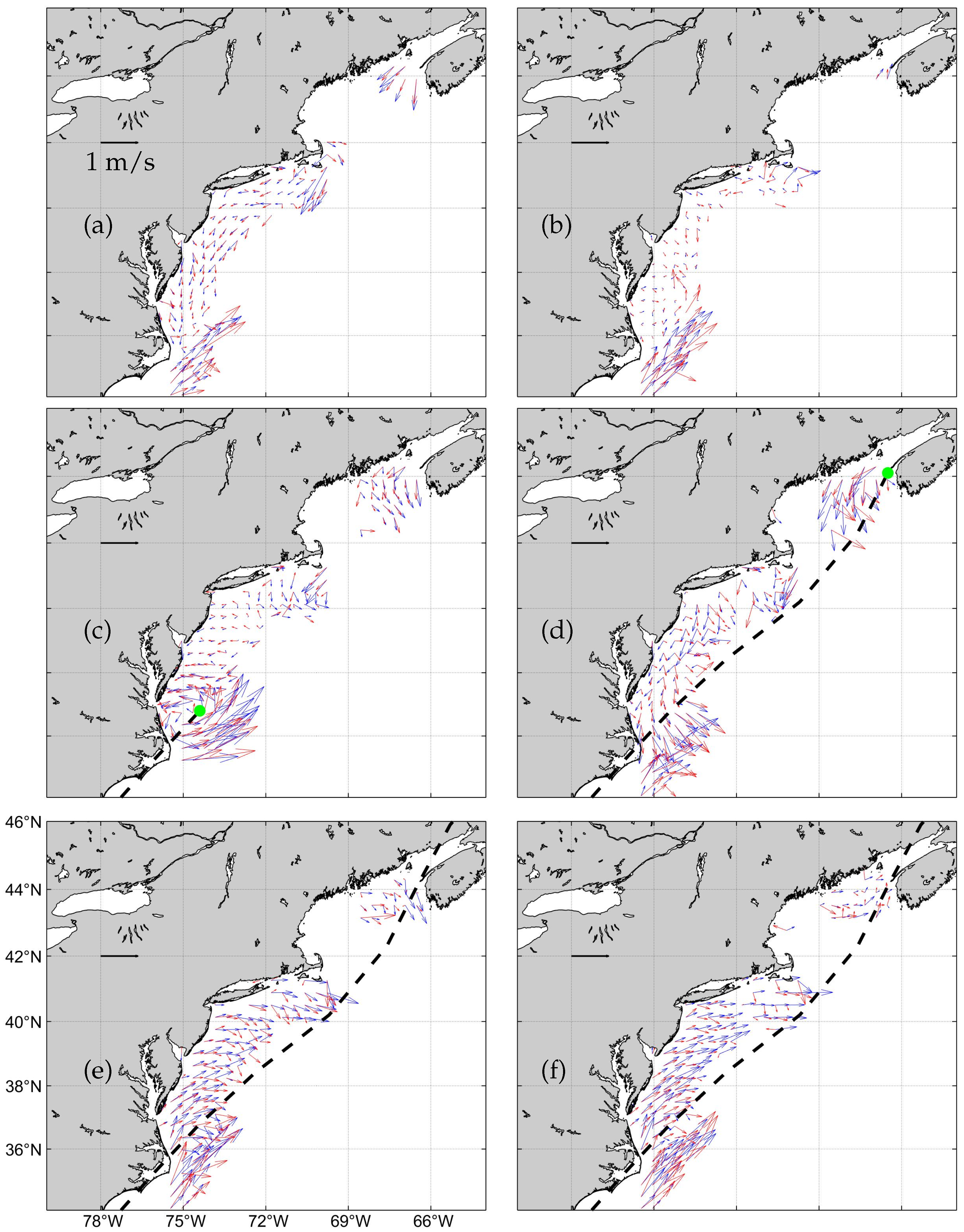
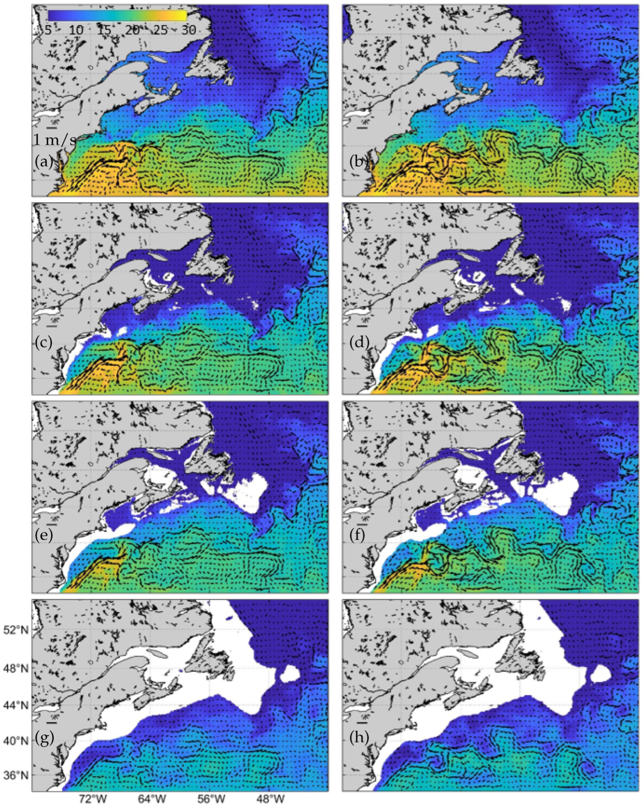
Since current measurements are very limited during this study period, the simulated currents are compared with counterparts in GLORYS to demonstrate the performance of CWMS-NWA. To properly validate the simulated currents, the weekly mean of both the simulated and observational currents during the pre-storm period (20–27 June) at several different depths are calculated from the results produced by CWMS-NWA and GLORYS (Figure 17). Both CWMS-NWA and GLORYS have a $1/12°$ resolution and can reproduce the general circulation, including the GuS and LaC. It should be mentioned however, that GLORYS includes data assimilation but does not include tides, WECs and high-resolution wind input for Hurricane Arthur.

The weekly-mean pre-storm circulation produced by CWMS-NWA and GLORYS features similar large-scale currents over the NWA, including the GuS and LaC. The GuS is much weaker away from the boundary towards the middle of the domain (between 48° and 64° W) in CWMS-NWA than in GLORYS (Figure 17a,b). By contrast, the LaC is stronger and much more defined in CWMS-NWA than GLORYS along the Newfoundland and Labrador Shelves and the slope of the Grand Banks. The eddies along the eastern edge of the model domain are different in CWMS-NWA than GLORYS reanalysis, especially over the region between 40° W and 48° W between 44° N and 48° N. Both CWMS-NWA and GLORYS have certain skills in simulating the NSC and SbC over the ScS and coastal currents in the Grand Banks, GSL and GoM. It should be noted, both CWMS-NWA and GLORYS have a 1/12° horizontal resolution and thus cannot resolve the small-scale features of the NSC or SbC. At 50 m depth, the coastal circulation is even weaker than at the surface (Figure 17c,d). At 50 m, the GuS is very similar in both CWMS-NWA and GLORYS. The LaC at 50 m is weaker that the counterpart at the surface in both CWMS-NWA currents and GLORYS. At 100 m, the LaC produced by CWMS-NWA is significantly weaker than the counterpart at 50 m. The LaC in GLORYS is also weaker at 100 m than the counterpart at 50 m, which is similar to CWMS-NWA. At 500 m, the LaC produced by CWMS-NWA is very similar to the currents in GLORYS (Figure 17e,f). The GuS is weak at 500 m in both CWMS-NWA and GLORYS. However, consistent with the surface and other depths, the GuS meanders are more defined in the open ocean in GLORYS than in CWMS-NWA.

The correlation is relatively low between the CWMS-NWA results and GLORYS. There is also slightly better agreement in the eastward component of the currents between CWMS-NWA and GLORYS than in the northward component. As mentioned above, the GLORYS reanalysis includes data assimilation while CWMS-NWA is prognostic without data assimilation. Another important difference is that CWMS-NWA includes tides and WCIs, while GLORYS does not. Thus, GLORYS lacks some important tidal-driven processes which are very important over our study region, particularly in the GSL, ScS, GoM and BoF. The wind velocity input in CWMS-NWA includes both background ERA5 wind and the high-resolution Moody’s HWind reanalysis. GLORYS does not use Moody’s HWind. Thus, GLORYS has less skills with large errors in the storm-induced currents. In addition, despite both CWMS-NWA and GLORYS having the same horizontal resolution of 1/12°, the topography is not necessarily the same and should lead to large differences in currents, particularly the directions. The above discussions suggest that GLORYS does not represent the true solution of 3D currents and hydrography over the NWA, particularly over the coastal and shelf waters.

4. Conclusions

The modified version of the coupled circulation-wave modelling system for the northwestern Atlantic (CWMS-NWA) was presented in this paper. The early version of CWMS-NWA was developed originally by Lin et al. [18] includes the VF and Bernoulli head, Stokes drift advection of tracers, wave-dissipation induced forces, WB driven-currents and impacts of surface waves on the bottom stress. Major modifications include a parameterization of LT following KC04 and the incorporation of WB within the MY25 vertical mixing scheme. Significant efforts were made in this paper in assessing the performance of CWMS-NWA in simulating surface waves, sea levels, three-dimensional (3D) currents and 3D hydrography over the NWA using satellite remote sensing data, in-situ observations and reanalysis over the study period.

A key part of this study was upgrading CWMS-NWA to include LT as well as WB within the MY25 vertical mixing scheme. The modified version of CWMS-NWA has satisfactory skills in simulating significant wave heights of surface waves and total sea levels over the coastal and shelf waters. Areas with both strong currents and large waves such as along the Gulf Stream or GoM during Hurricane Arthur showed smaller errors in the FC experiment. This highlights the importance of WCIs in regions with both currents and large waves. Large-scale circulation and hydrography are also simulated satisfactorily by the modified version of CWMS-NWA. Finally, the modified version of CWMS-NWA also has satisfactory skills in simulating storm-induced changes in currents and hydrography, particularly over areas affected by the storm.

Ocean responses to Hurricane Arthur (2014) were examined previously. McLaughlin et al. [17] simulated waves, storm surge and tides in the GoM-BoF system during this storm. Their coupled model included a two-way nested grid with a coarse resolution of 1000 m and a fine resolution of 500 m. However, their model domain was limited to the GoM and BoF and the hydrodynamic component was set to 2D mode. Cyriac et al. [50] investigated storm surge during Hurricane Arthur along the coast of North Carolina. They included Moody’s HWind along with the Generalized Asymmetric Holland Model (GAHM) and compared the wind speeds with buoy data. Their model includes an unstructured hydrodynamic model. It is coupled to SWAN and includes wave radiation stresses. While their model domain included the Caribbean Sea, Gulf of Mexico and entire western North Atlantic, it only has a fine resolution along the coast of North Carolina. Zhang et al. [51] also examined storm surge during Hurricane Arthur, with Weather Research and Forecasting (WRF) Model and the Finite Volume Coastal Ocean Model (FVCOM). They used a triply-nested model domain with resolutions ranging from 12 km in the outer domain over the western Atlantic. In their simulations, the horizontal resolution of FVCOM ranged from ∼1 km in the inner shelf to ∼10 km near the open boundaries. Despite coupling between an atmospheric model (WRF) and an ocean model (FVCOM), they did not include wave effects. The VF formalism is included as opposed to the wave radiation stress from Cyriac et al. [50]. Furthermore, LT, WB and the Wv. BBL are all accounted for in this model which is designed for advanced process-studies. The total sea level errors in our model results are comparable with other studies during Hurricane Arthur focused on coastal processes.

It is useful to quantify uncertainty of model results. As suggested by Mattern et al. [61], uncertainty analysis can be made using Monte Carlo techniques or emulator-based approaches if uncertainty is not built into the numerical model. Monte Carlo techniques require random samples to represent input uncertainty [62,63,64]. This is very computationally inefficient and not reasonable for 3D models [61]. Emulators on the other hand can use existing output to give a statistical approximation of unknown model output. They can do so by passing along the uncertainty from model inputs to model outputs [61,65,66]. Mattern et al. [61] used the emulator technique known as Polynomial chaos expansion. Via polynomial chaos, they were able to approximate model output probability distributions which in turn could be used to conduct uncertainty analysis. A follow-up study could be conducted to do a thorough uncertainty analysis of the model results. Mattern et al. [61] focused on biological inputs as well as some physical inputs such as freshwater river runoff, wind forcing, and mixing coefficients.

Major deficiencies of the coupled model used in this study include the coarse horizontal resolution of the model domain, the lack of three-way coupling with an atmospheric component and the absence of data assimilation to reduce errors arising from nonlinear horizontal circulation and turbulent vertical mixing processes. Future research is needed to improve the model performance by (a) enabling data-assimilation, (b) replacing the WB driven currents with surface wave modifications to the momentum flux from winds to surface currents and (c) including a surface wave-dependent surface roughness length within the vertical mixing scheme. Another WCI physical process that is not accounted for in the CWMS-NWA is non-breaking surface wave-induced mixing [67,68]. The Stokes drift could also be calculated using the full wave spectrum following the methodology suggested by Liu et al. [69]. Finally, other parameterizations of LT such as Harcourt [70] or Yu et al. [71] could improve the vertical mixing results. In the next project, CWMS-NWA will be used for a process-study to investigate and quantify WCIs in the NWA during Hurricane Arthur.

References

1. Sahoo, B.; Jose, F.; Bhaskaran, P.K. Hydrodynamic response of Bahamas archipelago to storm surge and hurricane generated waves—A case study for Hurricane Joaquin. Ocean Eng. 2019, 184, 227–238. [Google Scholar] [CrossRef]
2. Fedele, F.; Lugni, C.; Chawla, A. The sinking of the El Faro: Predicting real world rogue waves during Hurricane Joaquin. Sci. Rep. 2017, 7, 11188. [Google Scholar] [CrossRef] [PubMed]
3. Gutshabash, Y.S.; Lavrenov, I.V. Swell transformation in the cape Agulhas current. Izv. Atmos. Ocean. Phys. 1986, 22, 494–497. [Google Scholar]
4. Lavrenov, I.V. The wave energy concentration at the Agulhas Current off South Africa. Nat. Hazards 1998, 17, 117–127. [Google Scholar] [CrossRef]
5. Quilfen, Y.; Chapron, B. Ocean surface wave–current signatures from satellite altimeter measurements. Geophys. Res. Lett. 2019, 216, 253–261. [Google Scholar] [CrossRef]
6. Hegermiller, C.A.; Warner, J.C.; Olabarrietal, M.; Sherwood, C.R. Wave-current interaction between Hurricane Matthew wave fields and the Gulf Stream. J. Phys. Oceanogr. 2019, 49, 2883–2900. [Google Scholar] [CrossRef]
7. Marechal, G.; Ardhuin, F. Surface currents and significant wave height gradients: Matching numerical models and high-resolution altimeter wave heights in the Agulhas current region. J. Geophys. Res. Oceans 2021, 126, e2020JC016564. [Google Scholar] [CrossRef]
8. Zhou, X.; Hara, T.; Ginis, I.; D’Asaro, E.; Reichl, B.G. Evidence of Langmuir mixing effects in the upper ocean layer during tropical cyclones using observations and a coupled wave-ocean model. J. Geophys. Res. Oceans 2023, 128, e2023JC020062. [Google Scholar] [CrossRef]
9. Sun, R.; Cobb, A.; Villas Bôas, A.B.; Langodan, S.; Subramanian, A.C.; Mazloff, M.R.; Cornuelle, B.D.; Miller, A.J.; Pathak, R.; Hoteit, I. Waves in SKRIPS: WAVEWATCH III coupling implementation and a case study of Tropical Cyclone Mekunu. Geosci. Model Dev. 2023, 16, 3435–3458. [Google Scholar] [CrossRef]
10. Cao, Y.; Deng, Z.; Wang, C. Impacts of surface gravity waves on summer ocean dynamics in Bohai Sea. Estuarine Coast. Shelf Sci. 2019, 230, 106443. [Google Scholar] [CrossRef]
11. Peláez-Zapata, D.; Pakrashi, V.; Dias, F. Dynamics of Bubble Plumes Produced by Breaking Waves. J. Phys. Oceanogr. 2024, 54, 2059–2071. [Google Scholar] [CrossRef]
12. Wang, P.; Sheng, J. A comparative study of wave-current interactions over the eastern Canadian shelf under severe weather conditions using a coupled wave-circulation model. J. Geophys. Res. Oceans 2016, 121, 5252–5281. [Google Scholar] [CrossRef]
13. Bennis, A.; Ardhuin, F.; Dumas, F. On the coupling of wave and three-dimensional circulation models: Choice of theoretical framework, practical implementation and adiabatic tests. Ocean Modell. 2011, 40, 260–272. [Google Scholar] [CrossRef]
14. Craig, P.D.; Banner, M.L. Modeling wave-enhanced turbulence in the ocean surface layer. J. Phys. Oceanogr. 1994, 24, 2546–2559. [Google Scholar] [CrossRef]
15. Sun, Y.; Perrie, W.; Toulany, B. Simulation of wave-current interactions under hurricane conditions using an unstructured-grid model: Impacts on ocean waves. J. Geophys. Res. Oceans 2018, 123, 3739–3760. [Google Scholar] [CrossRef]
16. Chen, C.; Beardsley, R.C.; Cowles, G.; Qi, J.; Lai, L.; Gao, G.; Stuebe, D.; Liu, H.; Xu, Q.; Xue, P.; et al. An Unstructured Grid, Finite-Volume Community Ocean Model FVCOM User Manual, 4th ed.; Tech. Rep. 13–0701, NOAA/NWS/NCEP/MMAB; Univeristy of Massachusetts: Dartmouth, MA, USA, 2013; p. 404. [Google Scholar]
17. McLaughlin, C.; Law, B.; Mulligan, R. Modeling surface waves and tide-surge interactions leading to enhanced total water levels in a macrotidal bay. Coastal Eng. J. 2022, 64, 24–41. [Google Scholar] [CrossRef]
18. Lin, S.; Sheng, J.; Ohashi, K.; Song, Q. Wave-current interactions during Hurricanes Earl and Igor in the northwest Atlantic, practical implementation and adiabatic tests. J. Geophys. Res. Oceans 2021, 126, e2021JC017609. [Google Scholar] [CrossRef]
19. Warner, J.C.; Armstrong, B.; He, R.; Zambon, J.B. Development of a Coupled Ocean-Atmosphere-Wave-Sediment Transport (COAWST) Modeling System. Ocean Modell. 2010, 35, 230–244. [Google Scholar] [CrossRef]
20. Lin, S.; Sheng, J. Revisiting dependencies of the drag coefficient at the sea surface on wind speed and sea state. Cont. Shelf Res. 2020, 207, 104188. [Google Scholar] [CrossRef]
21. Madsen, O.S. Spectral wave-current bottom boundary layer flows. In Proceedings of the 24th International Conference on Coastal Engineering, Kobe, Japan, 23–28 October 1994; pp. 384–398. [Google Scholar] [CrossRef]
22. Warner, J.C.; Sherwood, C.R.; Arango, H.G.; Signell, R.P. Performance of four turbulence closure models implemented using a generic length scale method. Ocean Modell. 2005, 8, 81–113. [Google Scholar] [CrossRef]
23. Berg, R. Tropical Cyclone Report: Hurricane Arthur, 1–5 July 2014; Tech. Rep. AL012014, National Hurricane Center. 2015. p. 43. Available online: https://www.nhc.noaa.gov/data/tcr/AL012014_Arthur.pdf (accessed on 13 December 2021).
24. Hersbach, H.; Bell, B.; Berrisford, P.; Biavati, G.; Horányi, A.; Muñoz-Sabater, J.; Nicolas, J.; Peubey, C.; Radu, R.; Rozum, I.; et al. The ERA5 global reanalysis. Quart. J. Roy. Meteor. Soc. 2020, 123, 1–51. [Google Scholar] [CrossRef]
25. Copernicus Climate Change Service; Climate Data Store. ERA5 Hourly Data on Pressure Levels from 1940 to Present; Copernicus Climate Change Service (C3S) Climate Data Store (CDS). Available online: https://cds.climate.copernicus.eu/datasets/reanalysis-era5-pressure-levels?tab=overview (accessed on 15 August 2023). [CrossRef]
26. Hodges, K.; Cobb, A.; Vidale, P.L. How well are tropical cyclones represented in reanalysis datasets? J. Clim. 2017, 30, 5243–5264. [Google Scholar] [CrossRef]
27. Muis, S.; Lin, N.; Verlaan, M.; Winsemius, H.C.; Ward, P.J.; Aerts, J.C.J.H. Spatiotemporal patterns of extreme sea levels along the western North-Atlantic coasts. Sci. Rep. 2019, 9, 3391. [Google Scholar] [CrossRef]
28. Fan, Y.; Ginis, I.; Hara, T. The effect of wind–wave–current interaction on air–sea momentum fluxes and ocean response in tropical cyclones. J. Phys. Oceanogr. 2009, 39, 1019–1034. [Google Scholar] [CrossRef]
29. Egbert, G.D.; Erofeeva, S.Y. Efficient Inverse Modeling of Barotropic Ocean Tides. J. Atmos. Oceanic Technol. 2002, 19, 183–204. [Google Scholar] [CrossRef]
30. Fernandez, E.; Lellouche, J.M. Product User Manual for the Global Ocean Physical Reanalysis Product GLOBAL_REANALYSIS_PHY_001_030; CMEMS-GLO-PUM: Toulouse, France, 2018. [Google Scholar]
31. Drévillon, M.; Fernandez, E.; Lellouche, J.M. Product User Manual for the Global Ocean Physical Multi Year Product GLOBAL_MULTIYEAR_PHY_001_030; CMEMS-GLO-PUM, EU Copernicus Marine Service. 2023, p. 36. Available online: https://data.marine.copernicus.eu/product/GLOBAL_MULTIYEAR_PHY_001_030/description (accessed on 13 February 2023).
32. Marchesiello, P.; McWilliams, J.C.; Shchepetkin, A. Open boundary conditions for long-term integration of regional oceanic models. Ocean Modell. 2001, 3, 1–20. [Google Scholar] [CrossRef]
33. Kantha, L.H.; Clayson, C.A. On the effect of surface gravity waves on mixing in the oceanic mixed layer. Ocean Modell. 2004, 6, 101–124. [Google Scholar] [CrossRef]
34. Mellor, G.L.; Yamada, T. Development of a turbulence closure models for geophysical fluid problems. Rev. Geophys. 1982, 20, 851–875. [Google Scholar] [CrossRef]
35. Hughes, C.J.; Liu, G.; Perrie, W.; Sheng, J. Impact of Langmuir turbulence, wave breaking, and Stokes drift on upper ocean dynamics under hurricane conditions. J. Geophys. Res. Oceans 2021, 126, e2021JC017388. [Google Scholar] [CrossRef]
36. Mickael, A. GLOBMULTI_ERA5_GLOBCUR_01. IFREMER. 2020. Available online: https://sextant.ifremer.fr/record/857a3337-f59a-481a-bf98-5561e8b61e7b/ (accessed on 29 March 2022). [CrossRef]
37. Alday, M.; Accensi, M.; Ardhuin, F.; Dodet, G. A global wave parameter database for geophysical applications. Part 3: Improved forcing and spectral resolution. Ocean Modell. 2021, 166, 101848. [Google Scholar] [CrossRef]
38. Kumar, N.; Voulgaris, G.; Warner, J.C.; Olabarrieta, M. Implementation of the vortex force formalism in the coupled ocean-atmosphere-wave-sediment transport (COAWST) modeling system for inner shelf and surf zone applications. Ocean Modell. 2012, 47, 65–95. [Google Scholar] [CrossRef]
39. Feddersen, F.; Trowbridge, J.H. The effect of wave breaking on surfzone turbulence and alongshore currents: A modeling study. J. Phys. Oceanogr. 2005, 35, 2187–2203. [Google Scholar] [CrossRef]
40. Charnock, H. Wind stress on a water surface. Quart. J. Roy. Meteor. Soc. 1955, 81, 639–640. [Google Scholar] [CrossRef]
41. Fairall, C.W.; Bradley, E.F.; Hare, J.E.; Grachev, A.A.; Edson, J.B. Bulk Parameterization of Air–Sea Fluxes: Updates and Verification for the COARE Algorithm. J. Clim. 2003, 16, 571–591. [Google Scholar] [CrossRef]
42. Drennan, W.M.; Graber, H.C.; Hauser, D.; Quentin, C. On the wave age dependence of wind stress over pure wind seas. J. Geophys. Res. Oceans 2003, 108, 8062. [Google Scholar] [CrossRef]
43. Kantha, L.H.; Lass, H.U.; Prandke, H. A note on Stokes production of turbulence kinetic energy in the oceanic mixed layer: Observations in the Baltic Sea. Ocean Dyn. 2010, 60, 171–180. [Google Scholar] [CrossRef]
44. Martin, P.J.; Rogers, E.; Allard, R.A.; Dykes, J.D.; Hogan, P.J. Tests of Parameterized Langmuir-Circulation Mixing in the Ocean’s Surface Mixed Layer; NRL Memorandum Report NRL/MR/7320–13-9444; Naval Research Laboratory. 2013, p. 50. Available online: https://apps.dtic.mil/sti/pdfs/ADA589098.pdf (accessed on 1 May 2018).
45. Martin, P.J.; Savelyev, I.B. Tests of Parameterized Langmuir-Circulation Mixing in the Ocean’s Surface Mixed Layer II; NRL Memorandum Report NRL/MR/7320–17-9738, Naval Research Laboratory. 2017, p. 50. Available online: https://apps.dtic.mil/sti/pdfs/AD1038768.pdf (accessed on 30 April 2018).
46. The SWAN Team. SWAN User Manual Version 41.31; Delft University of Technology: Delft, The Netherlands, 2019; p. 135. [Google Scholar]
47. Pawlowicz, R.; Beardsley, B.; Lentz, S. Classical tidal harmonic analysis including error estimates in MATLAB using T_TIDE. Comput. Geosci. 2002, 28, 929–937. [Google Scholar] [CrossRef]
48. Zhang, H.; Sheng, J. Estimation of extreme sea levels over the eastern continental shelf of North America. J. Geophys. Res. Oceans 2013, 188, 6253–6273. [Google Scholar] [CrossRef]
49. Yang, S.; Sheng, J.; Ohashi, K.; Yang, B.; Chen, S.; Xing, J. Non-linear interactions between tides and storm surges during extreme weather events over the eastern Canadian shelf. Ocean Dyn. 2023, 73, 279–301. [Google Scholar] [CrossRef]
50. Cyriac, R.; Dietrich, J.C.; Fleming, J.G.; Blanton, B.O.; Kaiser, C.; Dawson, C.N.; Luettich, R.A. Variability in Coastal Flooding predictions due to forecast errors during Hurricane Arthur. Coastal Eng. J. 2018, 137, 59–78. [Google Scholar] [CrossRef]
51. Zhang, F.; Li, M.; Ross, R.C.; Lee, S.B.; Zhang, D.-L. Sensitivity Analysis of Hurricane Arthur (2014) Storm Surge Forecasts to WRF Physics Parameterizations and Model Configurations. Mon. Weather Rev. 2017, 32, 1745–1764. [Google Scholar] [CrossRef]
52. Merchant, C.J.; Embury, O.; Bulgin, C.E.; Block, T.; Corlett, G.K.; Fiedler, E.; Good, S.A.; Mittaz, J.; Rayner, N.A.; Berry, D.; et al. Satellite-based time-series of sea-surface temperature since 1981 for climate applications. Sci. Data 2019, 6, 223. [Google Scholar] [CrossRef] [PubMed]
53. Good, S.A.; Embury, O.; Bulgin, C.E.; Mittaz, J. ESA Sea Surface Temperature Climate Change Initiative (SST_cci): Level 4 Analysis Climate Data Record, Version 2.0.; Centre for Environmental Data Analysis: 2019. Available online: https://dx.doi.org/10.5285/aced40d7cb964f23a0fd3e85772f2d48 (accessed on 1 May 2022).
54. Smith, P.; Schwing, F. Mean circulation and variability on the Eastern Canadian continental shelf. Cont. Shelf Res. 1991, 11, 977–1012. [Google Scholar] [CrossRef]
55. Seidov, D.; Mishonov, A.; Parsons, R. Recent warming and decadal variability of Gulf of Maine and Slope Water. Limnol. Oceanogr. 2021, 66, 3472–3488. [Google Scholar] [CrossRef]
56. Boutin, J.; Vergely, J.-L.; Reul, N.; Catany, R.; Jouanno, J.; Martin, A.; Rouffi, F.; Bertino, L.; Bonjean, F.; Corato, G.; et al. ESA Sea Surface Salinity Climate Change Initiative (Sea_Surface_Salinity_cci): Weekly Sea Surface Salinity Product on a Global Grid, v04.41, for 2010 to 2022, NERC EDS Centre for Environmental Data Analysis. 2024. Available online: https://catalogue.ceda.ac.uk/uuid/0d0f4a942a144d9cab9263de3949a5d6 (accessed on 1 May 2022).
57. Gatien, M.G. A study in the Slope Water region south of Halifax. J. Fish. Res. Board Can. 1976, 33, 2213–2217. [Google Scholar] [CrossRef]
58. Petrie, B.; Drinkwater, K. Temperature and salinity variability on the Scotian Shelf and in the Gulf of Maine 1945–1990. J. Geophys. Res. 1993, 98, 20079–20089. [Google Scholar] [CrossRef]
59. Urrego-Blanco, J.; Sheng, J. Interannual Variability of the Circulation over the Eastern Canadian Shelf. Atmos.-Ocean 2012, 50, 277–300. [Google Scholar] [CrossRef]
60. Reul, N. Atlas of Tropical Cyclone Induced Wakes (2010–2020) (v1.0) for ESA Marine Atmosphere eXtreme Satellite Synergy project (MAXSS). Ver. 1.0. Ifremer, Plouzane, France. 2023. Available online: https://data-maxss.ifremer.fr/added_value/storm-wake/ibtracs/ (accessed on 1 March 2023).
61. Mattern, J.P.; Fennel, K.; Dowd, M. Sensitivity and uncertainty analysis of model hypoxia estimates for the Texas-Louisiana shelf. J. Geophys. Res. Oceans 2013, 118, 1316–1317. [Google Scholar] [CrossRef]
62. Clancy, D.; Tanner, J.E.; McWilliam, S.; Spencer, M. Quantifying parameter uncertainty in a coral reef model using Metropolis-Coupled Markov Chain Monte Carlo. Ecol. Model. 2010, 221, 1337–1347. [Google Scholar] [CrossRef]
63. Kim, S.; Samelson, R.M.; Snyder, C. Toward an uncertainty budget for a coastal ocean model. Mon. Weather Rev. 2010, 139, 866–884. [Google Scholar] [CrossRef]
64. Melbourne-Thomas, J.; Johnson, C.; Fulton, E. Characterizing sensitivity and uncertainty in a multiscale model of a complex coral reef system. Ecol. Model. 2011, 222, 3320–3334. [Google Scholar] [CrossRef]
65. Xiu, D.; Karniadakis, G.E. Modeling uncertainty in flow simulations via generalized polynomial chaos. J. Comput. Phys. 2003, 187, 137–167. [Google Scholar] [CrossRef]
66. Le Maître, O.L.; Knio, O.; Najm, H.; Ghanem, R. Uncertainty propagation using Wiener-Haar expansions. J. Comput. Phys. 2004, 197, 28–57. [Google Scholar] [CrossRef]
67. Dai, D.; Qiao, F.; Sulisz, W.; Han, L.; Babanin, A.V. An experiment on the nonbreaking surface-wave-induced vertical mixing. J. Phys. Oceanogr. 2010, 40, 2180–2188. [Google Scholar] [CrossRef]
68. Wu, L.; Rutgersson, A.; Sahlée, E. Upper-ocean mixing due to surface gravity waves. J. Geophys. Res. Oceans 2015, 120, 8210–8228. [Google Scholar] [CrossRef]
69. Liu, G.; Kumar, N.; Harcourt, R.; Perrie, W. Bulk, Spectral and Deep Water Approximations for Stokes Drift: Implications for Coupled Ocean Circulation and Surface Wave Models. J. Adv. Model. Earth Syst. 2021, 13, e2020MS002172. [Google Scholar] [CrossRef]
70. Harcourt, R. An Improved Second-Moment Closure Model of Langmuir Turbulence. J. Phys. Oceanogr. 2015, 45, 84–103. [Google Scholar] [CrossRef]
71. Yu, C.; Song, J.; Li, S.; Li, S. On an improved second-moment closure model for Langmuir turbulence conditions and its application. J. Geophys. Res. Oceans. 2022, 127, e2021JC018217. [Google Scholar] [CrossRef]
72. Lin, S.; Sheng, J. Assessing the performance of wave breaking parameterizations in shallow waters in spectral wave models. Ocean Modell. 2017, 20, 41–59. [Google Scholar] [CrossRef]
73. Lin, S.; Sheng, J.; Xing, J. Performance evaluation of parameterizations for wind input and wave dissipation in the spectral wave model for the northwest Atlantic Ocean. Atmos.-Ocean 2020, 58, 258–286. [Google Scholar] [CrossRef]
74. Pei, Q.; Sheng, J.; Ohashi, K. Numerical study of effects of winds and tides on monthly-mean circulation and hydrography over the southwestern Scotian Shelf. J. Mar. Sci. Eng. 2022, 10, 1706. [Google Scholar] [CrossRef]
75. Paduan, J.D.; Washburn, L. High-frequency radar observations of ocean surface currents. Annu. Rev. Mar. Sci. 2013, 5, 115–136. [Google Scholar] [CrossRef] [PubMed]
76. Stewart, R.H.; Joy, J.W. HF radio measurements of surface currents. Deep-Sea Res. Oceanogr. Abstr. 1974, 21, 1039–1049. [Google Scholar] [CrossRef]
77. Harlan, J.; Terrill, E.; Hazard, L.; Keen, C.; Barrick, D.; Whelan, C.; Howden, S.; Kohut, J. The Integrated Ocean Observing System high-frequency radar network: Status and local, regional, and national applications. Mar. Technol. Soc. J. 2010, 44, 122–132. [Google Scholar] [CrossRef]
78. Kohut, J.; Roarty, H.; Randall-Goodwin, E.; Glenn, S.; Lichtenwalner, C.S. Evaluation of two algorithms for a network of coastal HF radars in the Mid-Atlantic Bight. Ocean Dyn. 2012, 62, 953–968. [Google Scholar] [CrossRef]
79. Chapman, R.D.; Graber, H.C. Validation of HF radar measurements. Oceanography 1997, 10, 76–79. [Google Scholar] [CrossRef]
80. Fratantoni, P.S.; Pickart, R.S. The western north Atlantic Shelfbreak current system in summer. J. Phys. Oceanogr. 2007, 37, 2509–2533. [Google Scholar] [CrossRef]
81. Uchiyama, Y.; McWilliams, J.C.; Shchepetkin, A.F. Wave-current interaction in an oceanic circulation model with a vortex-force formalism: Application to the surf zone. Ocean Modell. 2010, 34, 16–35. [Google Scholar] [CrossRef]
Figure 1. Domain and bathymetry of the northwest Atlantic Ocean (NWA) for the coupled circulation–wave modelling system (CWMS-NWA). The “best track” for Hurricane Arthur in 2014 is shown by the solid red line with open red circles [23]. The blue x’s are the buoy locations and the green +’s are the tidal gauge stations. The magenta line extending from Halifax, Nova Scotia, is the location of the Halifax Line (HL).
Jmse 13 00239 g001
Figure 2. Time series of wind speeds (m/s) at five NDBC buoys from 00:00:00 28 June 2014 to 06:00:00 10 July 2014. Observation data are red and the blended wind speeds are black. The five buoys are (a) 41025, (b) 41036, (c) 44014, (d) 44024 and (e) 44066. Numbers in parentheses are the water depths of the buoys.
Jmse 13 00239 g002
Figure 3. Histograms of differences in wind speeds ( m / s ) between the blended wind and the buoy data at five NDBC buoys from 00:00:00 28 June 2014 to 06:00:00 10 July 2014. The five buoys are (a) 41025, (b) 41036, (c) 44014, (d) 44024 and (e) 44066. Numbers in parentheses are the water depths of the buoys.
Jmse 13 00239 g003
Figure 4. Time series of wind directions (°) at five NDBC buoys from 00:00:00 28 June 2014 to 06:00:00 10 July 2014. Observational data are red and the blended wind directions are black. Otherwise, as Figure 2.
Jmse 13 00239 g004
Figure 5. Wind roses ( m / s ) from (left) the observational wind data and (right) the blended winds at five NDBC buoys from 00:00:00 28 June 2014 to 06:00:00 10 July 2014. Wind roses for (a,b) Buoy 41025, (c,d) Buoy 41036, (e,f) Buoy 44014, (g,h) Buoy 44024, (i,j) Buoy 44066.
Jmse 13 00239 g005
Figure 6. Time series of the significant wave heights ( H s ) (m) at five NDBC buoys from 00:00:00 28 June 2014 to 06:00:00 10 July 2014. Black and green lines represent model results in runs FC and WO. Otherwise as in Figure 2.
Jmse 13 00239 g006
Figure 7. Time series of the differences in significant wave heights ( H s ) (m) between both the WO and FC experiments and the buoy data at five NDBC buoys from 00:00:00 28 June 2014 to 06:00:00 10 July 2014. Otherwise as in Figure 2.
Jmse 13 00239 g007
Figure 8. Time series of the smoothed peak wave periods (PWPs) ( T p ) (s) at five NDBC buoys from 00:00:00 28 June 2014 to 06:00:00 10 July 2014. Otherwise as in Figure 2.
Jmse 13 00239 g008
Figure 9. Time series of total surface elevations (m) at six tidal gauge stations from 00:00:00 1 June 2014 to 06:00:00 10 July 2014. The observed data are in red, the model results from runs FC and CO are black and green respectively. The six tidal gauge stations are (a) Yarmouth, (b) Halifax, (c) North Sydney, (d) Eastport, (e) Cutler Farris Wharf and (f) Bar Harbor.
Jmse 13 00239 g009
Figure 10. Time series of the tidal residuals (m) at six tidal gauge stations from 00:00:00 1 June 2014 to 06:00:00 10 July 2014. The observed data are in red, the model results from runs FC and CO are black and green respectively. The six tidal gauge stations are (a) Yarmouth, (b) Halifax, (c) North Sydney, (d) Eastport, (e) Cutler Farris Wharf and (f) Bar Harbor.
Jmse 13 00239 g010
Figure 11. Daily averaged SST (°C) on 22 May 2014 from (a) satellite observations (ESA CCI) and (b) model results produced by CWMS-NWA in run FC over the entire model domain. Weekly averaged (May 18-25, 2014) SSS based on (c) the satellite data (ESA CCI) and (d) model results in run FC over the entire model domain.
Jmse 13 00239 g011
Figure 12. Scatter plot of (a) the daily averaged SST (°C) on 22 May 2014 and (b) the weekly averaged SSS on 22 May 2014 based on simulated results and the ESA CCI project over the entire model domain.
Jmse 13 00239 g012
Figure 13. Vertical distributions of the two-day averaged (a) temperature (°C) and (b) salinity on 22 May 2014 based on model results in run FC (image) and AZMP data (colored circles) along the Halifax line transect.
Jmse 13 00239 g013
Figure 14. Vertical profiles of the two-day averaged (aj) temperature (°C) and (kt) salinity on 22 May 2014 data at the ten AZMP stations within 300 km of shore along the Halifax line. Red lines are from the AZMP data and black lines are interpolated model results from locations along the Halifax line from CWMS-NWA. Profiles are from closest to shore to seaward left to right: (a,k) ∼53 km, (b,l) ∼108 km, (c,m) ∼164 km, (d,n) ∼208 km, (e,o) ∼232 km, (f,p) ∼242 km, (g,q) ∼256 km, (h,r) ∼271 km, (i,s) ∼279 km, (j,t) ∼286 km from shore.
Jmse 13 00239 g014
Figure 15. Distributions of (top) pre-storm SST (a) based on satellite observations and (b) model results in run FC, (middle) post-storm SST (c) based on satellite observations and (d) model results in run FC and (bottom) storm-induced SST changes ( Δ s t SST) (°C) based on (e) satellite observations and (f) model results in run FC over the entire model domain. SST color increments every 2.5 °C and Δ s t SST color increments every 1.0 °C.
Jmse 13 00239 g015
Figure 16. Scatter plots of (a) S S T p r e , (b) S S T p o s t and (c) Δ s t S S T (°C) between MAXSS satellite observations and model results over the entire model domain.
Jmse 13 00239 g016
Figure 17. Weekly mean (20–27 June) temperature (°C) and currents (m/s) from (a,c,e,g) CWMS-NWA and (b,d,f,h) GLORYS at the (top row) surface, (second row) 50 m, (third row) 100 m and (bottom row) 500 m.
Jmse 13 00239 g017