Article

Dynamic Target Hunting Under Autonomous Underwater Vehicle (AUV) Motion Planning Based on Improved Dynamic Window Approach (DWA)

1
Key Laboratory of Underwater Robot Technology, Harbin Engineering University, Harbin 150001, China
2
College of Intelligent Systems Science and Engineering, Harbin Engineering University, Harbin 150001, China
*
Author to whom correspondence should be addressed.
J. Mar. Sci. Eng. 2025, 13(2), 221; https://doi.org/10.3390/jmse13020221
Submission received: 26 December 2024 / Revised: 17 January 2025 / Accepted: 23 January 2025 / Published: 24 January 2025
(This article belongs to the Section Ocean Engineering)

Abstract

:
A dynamic distributed target hunting method is proposed for the problem of distributed moving target hunting by multiple Autonomous Underwater Vehicles (AUVs). By integrating the improved Dynamic Window Approach (DWA) with the Rapidly-exploring Random Tree (RRT) algorithm and incorporating collision avoidance rules between AUVs into the evaluation system of the DWA, the collision avoidance rules are quantified, and corresponding evaluation functions are established. This allows for the selection of motion trajectories that comply with the collision avoidance rules from the predicted trajectory set, improving the obstacle avoidance capability during AUV motion planning and enhancing the reliability of the target hunting task. The introduction of a consistency algorithm maintains the consistency of the group task information and ensures that the hunting strategy can be adjusted promptly in the event of an AUV failure, allowing the target hunting task to continue. Polynomial regression algorithms are used to predict the moving target’s trajectory. Based on a polygonal hunting formation, the hunting potential points are dynamically allocated, and, finally, each AUV executes distributed motion planning towards the hunting potential points to form the hunting formation. Simulation results show that the proposed method achieves efficient multi-AUV-distributed dynamic target hunting.

1. Introduction

The Autonomous Underwater Vehicle (AUV) is a complex system integrating sensor detection, information fusion, vehicle control, and other technologies and has no physical connection with the mother ship [1]. AUVs can play an increasingly important role in the exploration and exploitation of marine resources, and AUVs can fulfill a wide range of underwater tasks in both civil and military applications [2]. Motion planning is the foundation of AUVs for underwater missions, but underwater environments are harsh, with not only static but also dynamic obstacles, so it is important for AUVs to have localized planning capabilities [3]. AUVs can accomplish many tasks once motion planning is achieved, such as dynamic target hunting tasks, which have an important role in the military field [4].
The Artificial Potential Field (APF) [5], Velocity Obstacle (VO) [6], Dynamic Window Approach (DWA) [7], and Time Elastic Band (TEB) [8] algorithms can all be used for autonomous collision avoidance in robots. Among them, the DWA algorithm has dynamic planning capabilities, but its collision avoidance performance is poor in complex environments [9]. Molinos et al. proposed the DW4DO algorithm and the DW4DOT algorithm to handle dynamic obstacles. These algorithms increase the data dimensions stored in the grid and can predict multiple velocities, making dynamic obstacle avoidance safer and more efficient compared to basic algorithms [10]. Liu et al. optimized the trajectory evaluation function of the DWA algorithm to guide the DWA algorithm for local path planning and dynamic obstacle avoidance by using the critical nodes extracted from the global path planned by the A* algorithm [11]. Song et al. used an improved ant colony algorithm for global path planning in static environments and then improved the DWA algorithm by removing redundant nodes, optimizing the initial direction, and improving the evaluation function to achieve path planning in the case of avoiding static obstacles and dynamic obstacles [12]. By analyzing the above literature, it can be concluded that reference [10] can predict multiple velocities, but it still does not fully cover the entire dynamic window. The improved DWA algorithm proposed in reference [11] achieves better obstacle avoidance, but its performance in avoiding unknown dynamic obstacles is poor, leading to a higher risk of collisions. Reference [12] suggests combining the ant colony algorithm with DWA, which works well in known environments but is not suitable for environments with unknown obstacles.
The advantage of the RRT algorithm lies in its ability to efficiently find feasible paths in high-dimensional, complex, and unknown environments [13]. Wang et al. proposed the HA-RRT algorithm, which realizes two-dimensional path planning by introducing dynamic factors to improve the convergence efficiency of the algorithm as well as adaptive adjustment strategies to adapt to the complex marine environment [14]. Li et al. proposed an algorithm combining DWA and RRT to realize path planning in complex static obstacle environments by improving the period of the whole dynamic window to generate the velocity space and planning the guidance points in the localized region with the RRT algorithm [15]. From the analysis of the above literature, it can be concluded that the RRT algorithm can perform path planning to avoid obstacles and reach the global goal point in unknown environments. However, the generated path does not consider the constraints of the moving objects, and, in some cases, the robot may not be able to follow the planned path completely, leading to task failure. Additionally, the algorithm lacks the ability to avoid dynamic obstacles.
In terms of dynamic target hunting technology, the research not only includes accurate prediction of the target’s trajectory but also covers how AUV groups work together to form a hunting formation and how to adjust tactics and strategies when the target dynamics change to ensure mission success.
In the area of moving target trajectory tracking and prediction, Zhu et al. developed a set of target trajectory prediction models based on LSTM networks, which can predict the posture in the battlefield environment and provide tactical decision-making references for combatants [16]. Wang et al. developed a modified Mean Shift tracking algorithm to solve the difficult problem of position prediction when the target is fast moving or occluded and accurately predicted the position by inter-frame clustering motion and scale estimation [17]. Zhang et al. proposed a heterogeneous model integration method of the inverse optimization propagation neural network and physical model for whale algorithm (WOA) optimization, which can predict the underwater position and surface position of an underwater glider [18]. It can be seen that advances in trajectory prediction techniques are closely dependent on artificial intelligence algorithms, especially neural-network-based methods, which in turn cannot succeed without adequate training data.
In terms of target interception point computation, Meng et al. proposed a prediction and planning-based interception algorithm in the field of harbor protection, which mainly operates on potentially hazardous targets approaching the harbor, where an artificial potential field algorithm is utilized to design the interception path. In addition, the authors consider the influence of environmental factors such as the direction and speed of the sea currents and propose corresponding coping strategies [19]. Lan et al. proposed a distributed control strategy for the multi-target interception problem of evacuation targets, using a dynamic assignment method to assign a tracking robot to each target. By analyzing the target trajectory and the movement paths of other robots, the interception target of each robot is determined, and a one-to-one interception task is performed [20]. Tahir et al. adopted an improved proportional navigation guidance algorithm to intercept maneuvering targets by estimating the acceleration of the maneuvering target through a prediction algorithm, estimating the target state after obtaining the acceleration information, and then performing the interception [21].
The article proposes the following basic assumptions:
  • Assumption 1: Obstacles and AUVs are on the same horizontal plane.
  • Assumption 2: AUVs can obtain environmental information using sonar and other sensor equipment, including the positions of obstacles and the size and speed of dynamic obstacles.
  • Assumption 3: AUVs navigate along the planned path, and their motion parameters are consistent with the planned parameters.
  • Assumption 4: The motion state information of AUVs, including position, heading angle, and speed, can be shared within the cluster.
Existing hunting research emphasizes inter-robot collaborative approaches to enhance hunting efficiency and reduce resource waste. For potential collision risks, traditional local planning strategies such as artificial potential fields are mostly used to avoid them, the motion planning is ineffective, the prediction accuracy and validity of interception points need to be improved, and the strategy of the hunting formation needs to be improved. Aiming at the above problems, this paper proposes a dynamic target hunting strategy under AUV motion planning based on improved DWA. The main innovations include the following:
  • A motion planning algorithm based on improved DWA is proposed to enhance the collision avoidance performance of AUVs in complex static obstacle environments and dynamic obstacle environments.
  • Setting up multi-AUV-distributed collision avoidance rules and integrating them into the evaluation system of DWA, quantifying the collision avoidance rules, and establishing the corresponding rule evaluation function so as to optimize the motion trajectories conforming to the collision avoidance rules among the predicted set of trajectories.
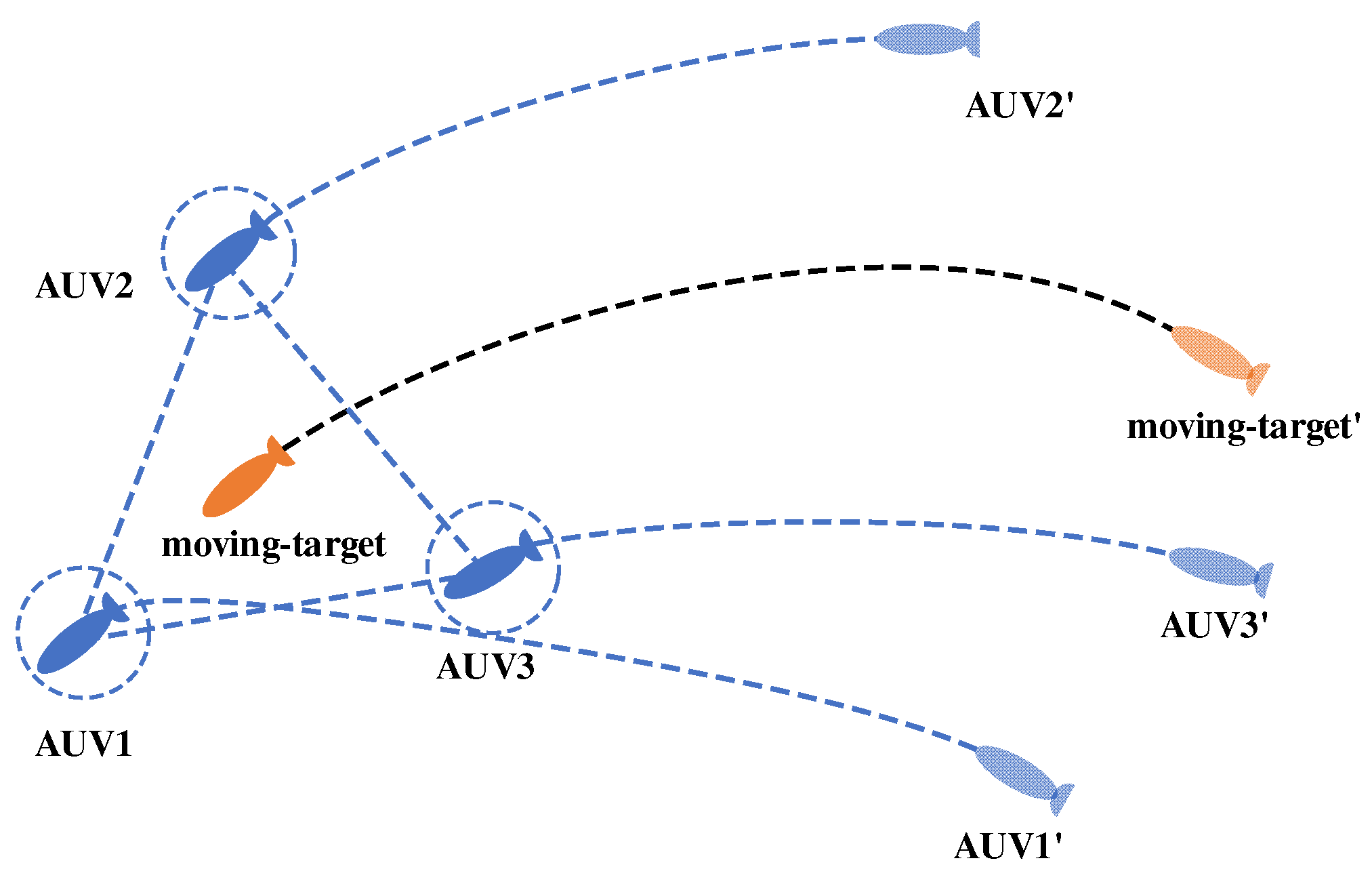
  • A consistency algorithm is introduced to ensure the consistency of multi-AUV information and mission continuity in the case of leader failure. Dynamic target trajectories are predicted by polynomial regression, and hunting potential points are dynamically assigned according to the polygonal hunting formation, which is formed by combining the distributed motion planning of each AUV.

2. Task Element Modeling

2.1. AUV Kinematic Modeling

This paper simplifies the modeling by taking the Minesniper MkII torpedo-type AUV as the research object [22], and an AUV kinematic model was introduced. Define S k = x k , y k , φ k as the AUV state vector. In the above equation, x k , y k represents the position of the AUV at moment k , and φ k represents the AUV bow angle. The AUV kinematic equation can be simplified to S k + 1 = S k + 1 + f S k , v k , φ ˙ k , and
f S k , v k , φ ˙ k = v k + v ˙ k cos φ k + φ ˙ k Δ t Δ t v k + v ˙ k sin φ k + φ ˙ k Δ t Δ t φ k + φ ˙ k Δ t
In the equation, v k represents the velocity of AUV movement, v ˙ k represents the acceleration of AUV movement, and φ ˙ k represents the angular velocity of AUV movement. The following are the kinematic constraints of the AUV in this paper:
0 v k 2 π 3 φ ˙ k π 3

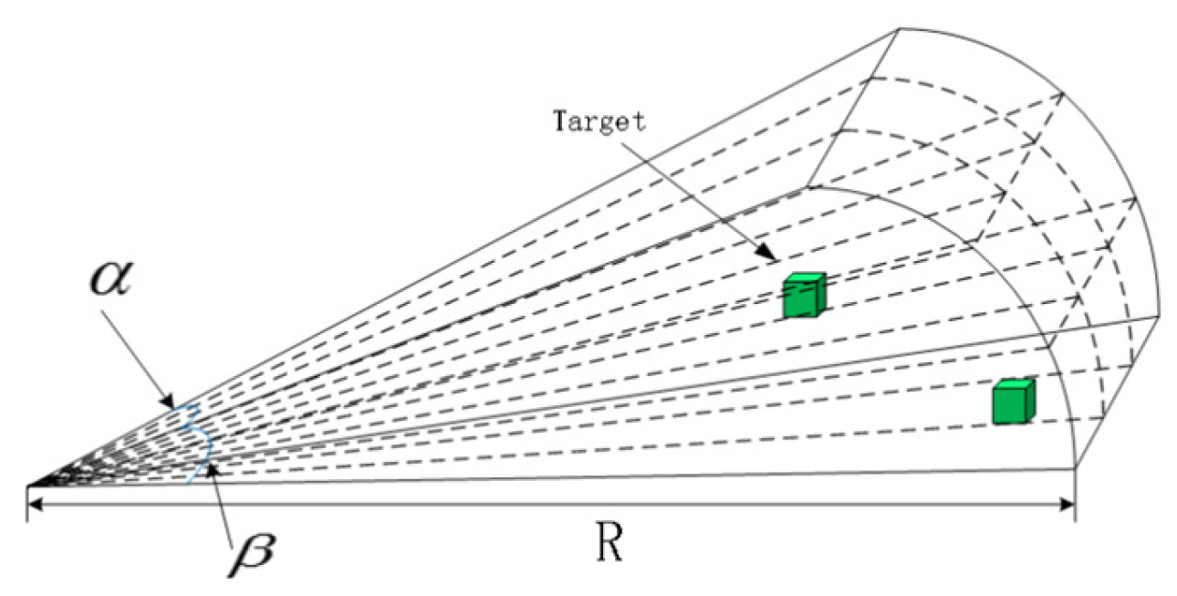
2.2. Forward-Looking Sonar Detection Model

Considering the underwater environment, a mathematical model was developed based on the working principle of sonar [23]. Therefore, in this paper, the radius of detection of the forward-looking sonar equipped by the navigator is 100 m in which the horizontal detection angle is 120°, the operating frequency is 2 KHz, and the method of matrix array statistics is used to deal with the information within the range of the sonar opening angle. The forward-looking sonar can be simply expressed as shown in Figure 1:
Objects that meet the following conditions can be detected by sonar:
y t x t 2 + y t 2 sin α 2 x t 2 + y t 2 R
Additionally, ( x t , y t ) can be expressed as follows:
x t = x x 0 y t = y y 0
In the equation, ( x , y ) is the coordinates of the target in the hull coordinate system.
In addition, ( x 0 , y 0 ) is the coordinates of the AUV configured sonar in the hull coordinate system, and ( x t , y t ) indicates the relative position of the target in relation to this AUV.

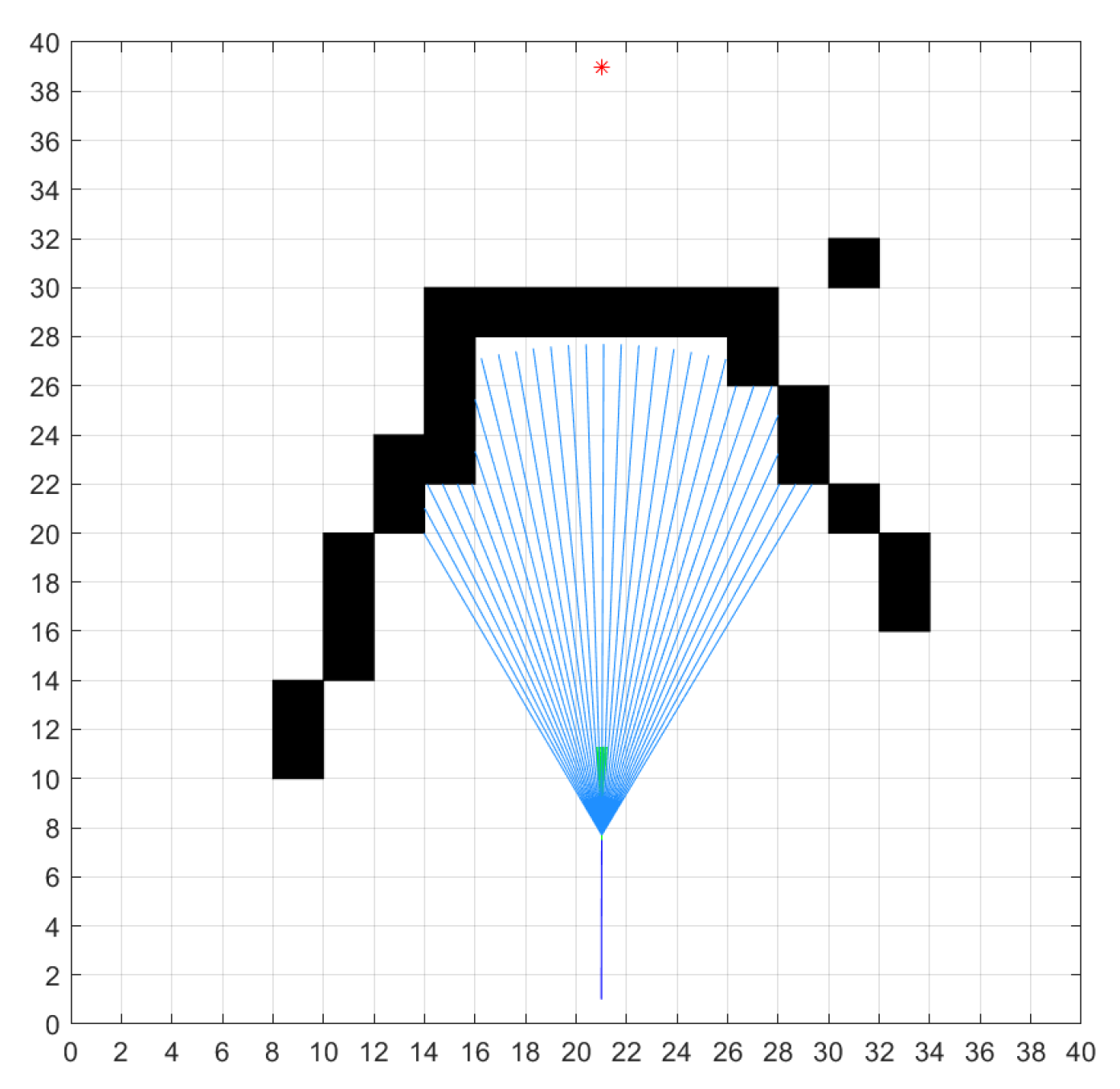
2.3. Static Obstacle Modeling

This paper uses grid map modeling and distinguishes between passable and impassable areas using black and white colors. The former represents obstacle regions, while the latter represents feasible areas. The obstacle model consists of irregular single or continuous static grids, which can simulate complex underwater environments with obstacles [24].

2.4. Dynamic Obstacle Modeling

In order to enhance the safety of avoiding dynamic obstacles, the dynamic obstacle is expanded into a circle of equal diameter based on its body length, and assuming that the motion is linear in the localized region, the kinematic equation can be expressed as follows:
x k + 1 x ˙ k + 1 y k + 1 y ˙ k + 1 = 1 T 0 0 0 1 0 0 0 0 1 T 0 0 1 1 x k x ˙ k y k + 1 y ˙ k + 1 + 1 0 0 0 1 1 0 0 0 0 1 0 0 0 1 1 ω k x ¨ k ω k y ¨ k
In the equation, x k , x ˙ k , and x ¨ k represent the position, velocity, and acceleration of the target in the x-axis direction at moment k; y k , y ˙ k , and y ¨ k represent the position, velocity, and acceleration of the target in the x-axis direction at moment k; ω k is Gaussian white noise; T is the sampling time.

3. Obstacle Avoidance Motion Planning for AUV Based on DWA and RRT

3.1. Basic DWA Algorithm

The basic DWA selects the optimal trajectory to maximize the distance between the robot and obstacles, maximize speed, and achieve a heading closest to the target [25]. The robot moves with the velocity combination of the selected trajectory into the next motion cycle. This process is repeated to achieve online real-time motion planning. The pseudocode for the DWA algorithm (Algorithm 1) is as follows:
Algorithm 1 Dynamic Window Approach
Input: current position robotPose, target point robotGoa, model parameter robotModel
Output: motion trajectory dataset robotTrajectory
1: BEGIN
2:   desiredV = calculateV(robotPose,robotGoal)
3:   laserscan = readScanner()
4:   allowable_v = generateWindow(robotV, robotModel)
5:   allowable_w = generateWindow(robotW, robotModel)
6:   for each v in allowable_v
7:     for each w in allowable_w
8:     dist = find_dist(v,w,laserscan,robotModel)
9:     breakDist = calculateBreakingDistance(v)
10:    if (dist > breakDist)
11:     heading = hDiff(robotPose,goalPose, v,w)
12:     clearance = (dist − breakDist)/(dmax − breakDist)
13:     cost = costFunction(heading,clearance, abs(desired_v −v))
14:       if (cost > optimal)
15:       best_v = v
16:       best_w = w
17:       optimal = cost
18:  set robotTrajectory to best_v, best_w
19:END
The functions in the code are explained as follows:
DWA(): The main function of the DWA algorithm.
calculateV(): Calculates the desired velocity based on the robot’s current position and the target position.
readScanner(): Reads data from the distance sensor and returns information about obstacles in the surrounding environment.
generateWindow(): Generates a feasible velocity window based on the current speed and the robot’s model.
generateWindow(): Generates a feasible angular velocity window based on the current angular velocity and the robot’s model.
find_dist(): Calculates the safe driving distance where the robot will not collide with any obstacles using sensor data and the robot’s model.
calculateBreakingDistance(): Computes the distance required for the robot to come to a complete stop.
hDiff(): Evaluates the heading cost as the angular difference between the robot’s heading and the target position for a given velocity and angular velocity.
costFunction(): Calculates a total evaluation value by considering the heading cost, obstacle clearance cost, and the cost of the difference between the current velocity and the desired velocity.

3.2. Improvement of Velocity Space

Traditional DWA limits velocity space to the first motion cycle, potentially missing feasible trajectories. In the dynamic window, the improved DWA algorithm expands the reachable velocity range of a single motion cycle to the reachable velocity range of all motion cycles as the velocity space. This improvement can significantly increase the number and breadth of assessable trajectories within each prediction cycle. The following equation is for improving the speed space:
V w = v w , ω w T
and
v w max 0 , v a 0 a T , min v max , v a 0 + a T ω w max ω max , ω a 0 α T , min ω max , ω a 0 + α
In the above equation, v w and ω w are the AUV velocity and bow angular velocity in the dynamic window, v a 0 and ω a 0 are the initial AUV velocity and bow angular velocity in the window, a and α are the maximum acceleration of the AUV and the maximum bow angular acceleration, v max is the maximum velocity of the AUV, T is the prediction period, max(∙) is the function of maximum value, and min(∙) is the function of minimum value.
After generating the velocity space, samples are taken at a sampling rate of ls , and each sampling velocity state V s = v s , ω s is taken as the expected velocity state of a trajectory. Combined with the AUV motion model, trajectories within the prediction period are generated.

3.3. Obstacle Sampling Window

Conventional DWA can stagnate in complex or confined spaces [26], and it is not possible to plan a path to bypass the obstacles. To address this issue, this paper proposes an obstacle sampling window, as shown in Figure 2, where the red asterisk represents the target point and the blue lines represent the sampling lines, which also reflect the sonar-detectable area. The obstacle sampling window is used to determine whether the AUV will encounter concave continuous obstacles and predict if it may lead to the AUV becoming stagnant. The formula for the obstacle sampling window space is as follows:
S w = θ w , d w T θ w 0 , θ r 0 , 2 π θ r , d w [ 0 , ρ ]
In the above equation, θ w is the sampling angle; d w is the sampling distance; θ r is the opening angle parameter; ρ is the distance parameter.
If the sampling line intersects with the obstacle, it is defined as l o i = 1 . The occupancy value of the obstacle window is as follows:
F a = 1 , i = 1 2 θ r θ w + 1 | l o i 1 | = 0 0 ,   otherwise  
In the above equation, l o i is the occupancy value of the sampling line. When F a = 1 , if the AUV continues moving in the current direction, it will not be able to avoid the obstacle and will become stagnant.

3.4. Complex Static Obstacle Avoidance Incorporating SAGRRT

In order to overcome DWA’s limitations in complex environments, this section proposes the SAGRRT algorithm. The SAGRRT algorithm, when there is a risk of stagnation for the AUV, uses guidance points to guide DWA in planning the path, thereby escaping complex obstacles and achieving efficient obstacle avoidance.

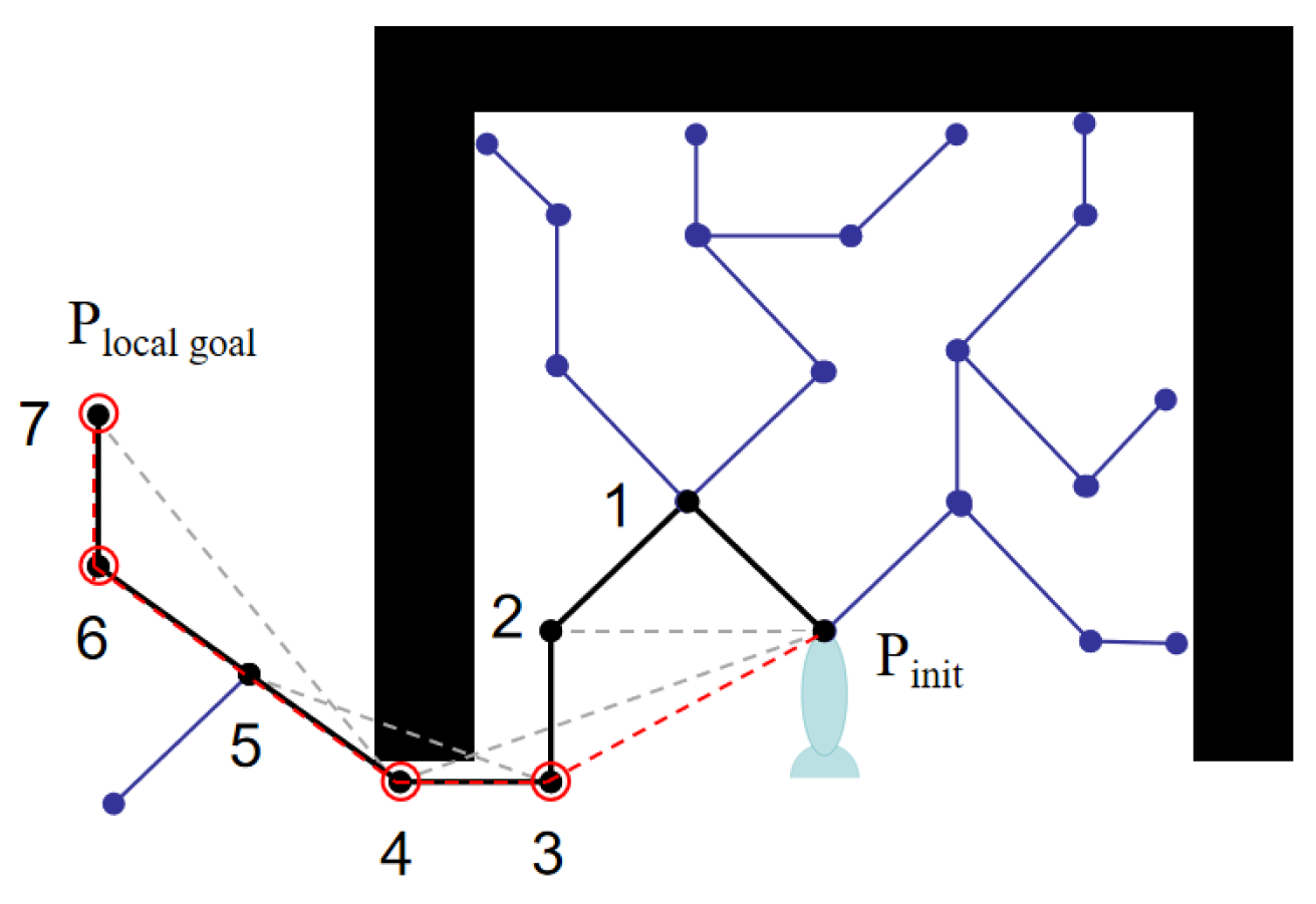
3.4.1. SAGRRT Static Obstacle Avoidance Guidepost Planning

When there is a risk of stagnation, SAGRRT searches for feasible region nodes, and the nodes are used as local target points P l o c a l   goal . As shown in Figure 3, all the guidance points are composed of all the connected nodes in the path from P l o c a l   goal to P n o w .

3.4.2. Extraction Rules for Key Guiding Points

This paper proposes a key point selection rule to eliminate redundant guide points. The principle is shown in Figure 4; between the start point and point 7, starting from the starting point, the path between each pair of guide points is checked in turn. If the path does not collide with an obstacle, the previous guide point is redundant. If a collision occurs at a connection, the previous guide point is the critical point, and the checking of subsequent connections continues from that point. Traversing all of the guide points generates the set of critical guide points {3, 4, 6, 7}, as shown in Figure 4.

3.5. Dynamic Obstacle Avoidance Incorporating DAGRRT

The traditional DWA struggles with fast-moving obstacles due to its short-sighted trajectory prediction. In order to solve this problem, this section proposes a dynamic obstacle avoidance method incorporating the DAGRRT algorithm, which introduces the DAGRRT algorithm to plan local guidance points when it is determined that the DWA algorithm cannot effectively avoid dynamic obstacles. The DAGRRT algorithm uses safety guidance points as the target points for DWA, which can plan safer dynamic obstacle avoidance trajectories.
The dynamic obstacle is first inflated to a circle with its volume length as the diameter, and then the forward space of the dynamic obstacle is divided into three regions based on the relative state between the AUV and the dynamic obstacle: the collision risk region, the collision danger region, and the safety region.
If the AUV enters the collision risk area, it means that it has the risk of collision with dynamic obstacles. If the AUV enters the collision risk zone, the current velocity, maximum acceleration, and relative velocity of the AUV to the obstacle need to be taken into account to calculate the minimum distance threshold that should be maintained between the AUV and the obstacle d s , which is expressed as follows:
d s = v o v max + v o a + t ω + 2 d o a + v max 2 + v o 2 2 a + d p
In the equation, d o is the diameter of the dynamic obstacle expansion circle; d p is the distance threshold adjustment parameter; t ω is the time required for the AUV to complete all steering maneuvers. The expression is as follows:
t ω = 3 π 2 ω + 2 ω α , α > π 2 ω 2 π α + 4 π α ,   otherwise  
ω represents the angular velocity of AUV, and α represents the angular acceleration of AUV.
When the AUV enters the boundary of the hazardous area, the DAGRRT algorithm plans dynamic obstacle avoidance guide points, and the principle is shown in Figure 5. The search node is discarded if it is within the hazardous area; on the contrary, this node is set as the local goal point P l o c a l   goal of dynamic obstacle avoidance, and a set of dynamic obstacle avoidance guide points is established by backtracking the path nodes, which is used to guide the planning algorithm to avoid the dynamic obstacles safely.

4. Introduction of DAGRRT Dynamic Obstacle Avoidance

We propose a distributed collision avoidance framework for AUVs using an improved DWA. This framework employs a standardized rule-based approach to ensure safe and efficient multi-AUV operations. This framework can improve the safety and efficiency of collision avoidance planning between multiple AUVs.

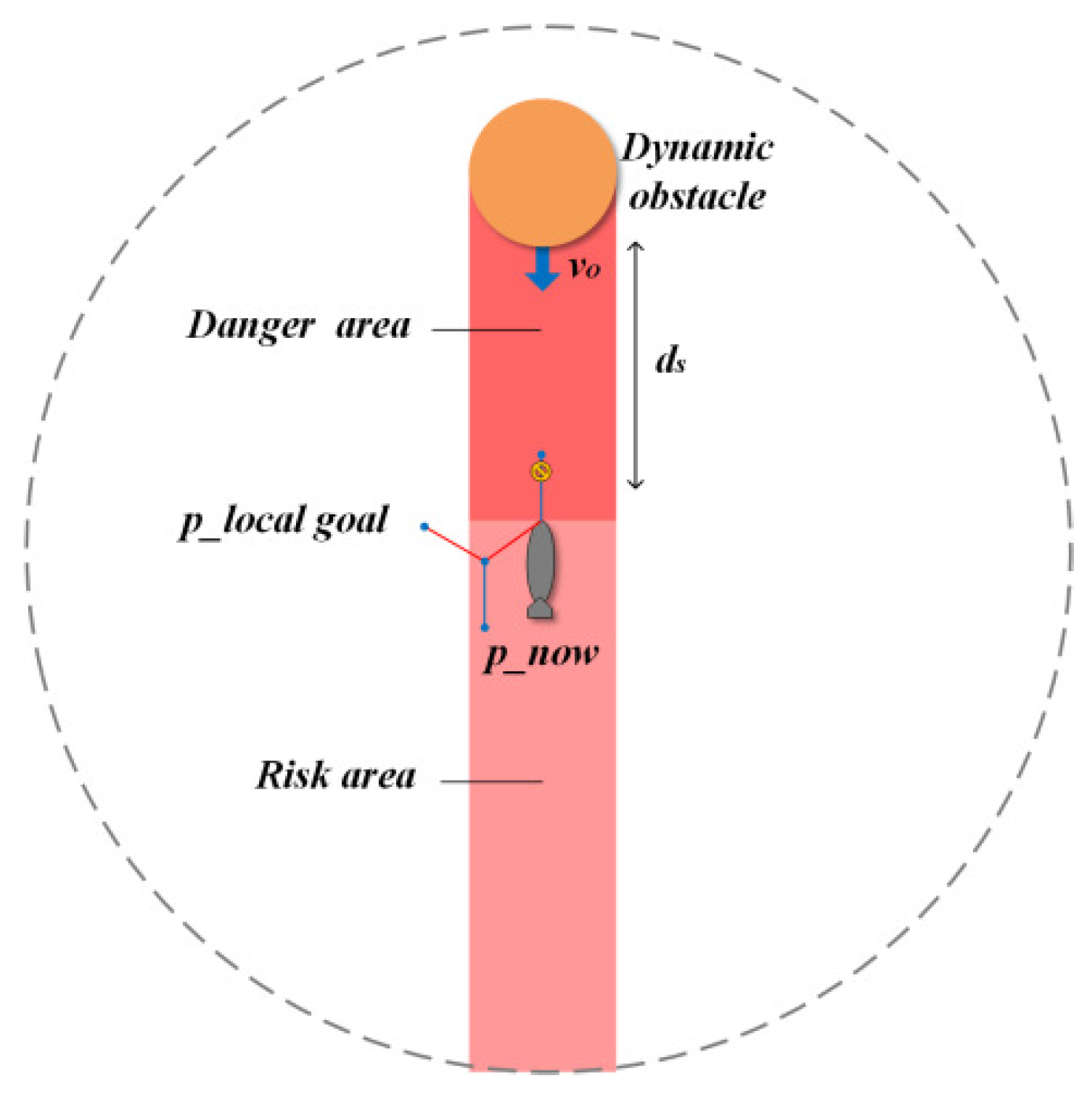
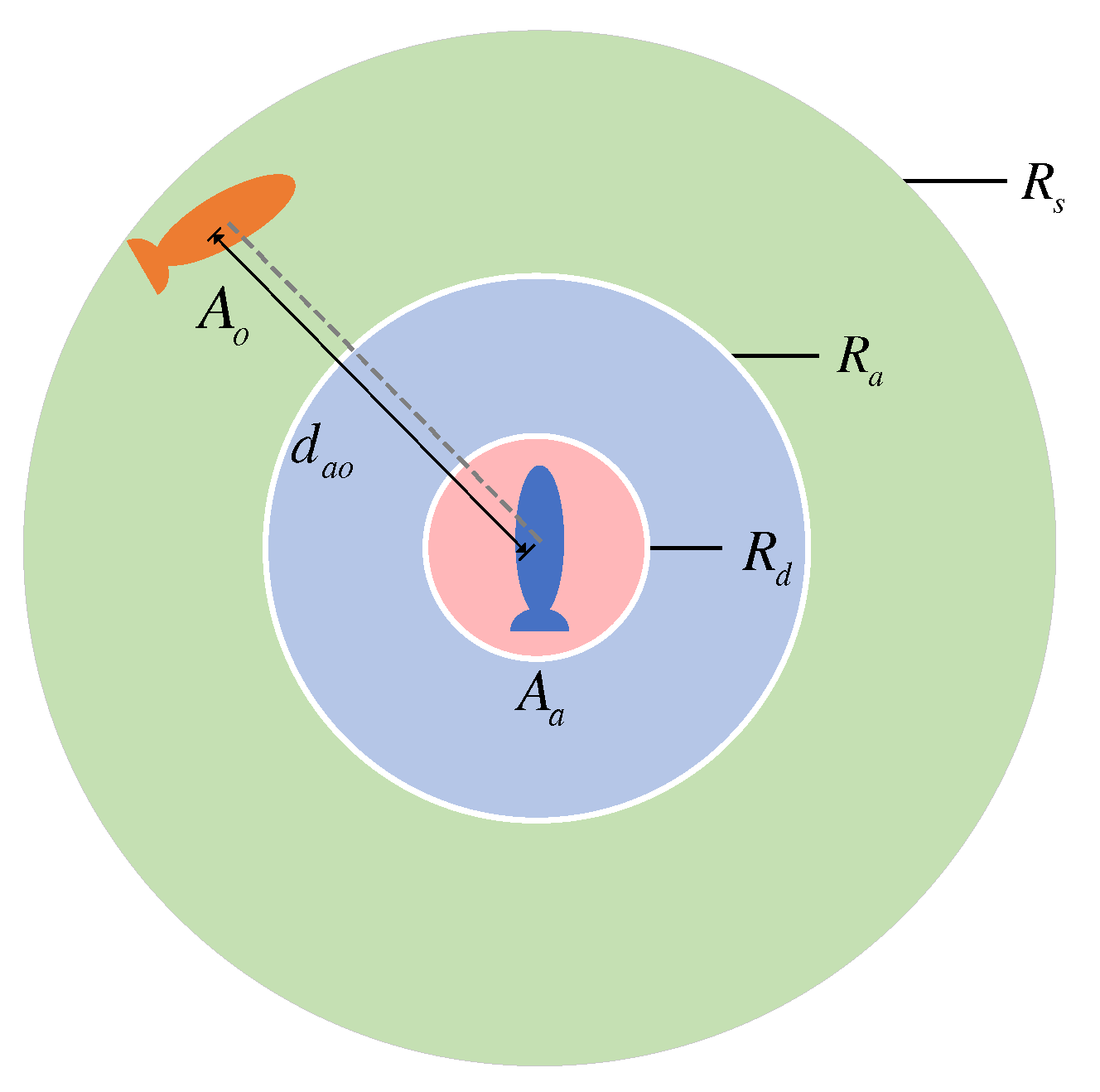
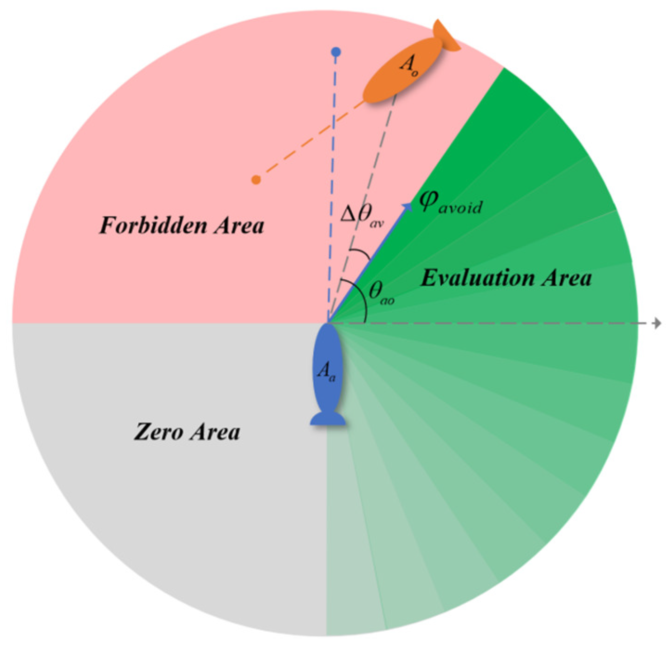
4.1. Bump Avoidance Space Division

The space around the AUVs is divided into three different areas as shown in Figure 6: safe space, risk space, and collision space. R s , R a , and R d , respectively, correspond to the boundaries of safety space, risk space, and collision space in the risk space division. When the distance between two AUVs is d a o ( R s , + ) , it is in the safe space, and no active collision avoidance is required; when d a o ( R d , R s ] , it is in the risk space, and active collision avoidance is performed when there is a risk of collision avoidance; when d a o ( R d , R a ] , it is necessary to comply with the rules of collision avoidance; and when d a o R d , it is regarded as a collision. By dividing the collision avoidance space and setting the threshold value, the multi-AUV system can significantly improve the safety of collision avoidance while guaranteeing the efficiency of task execution.

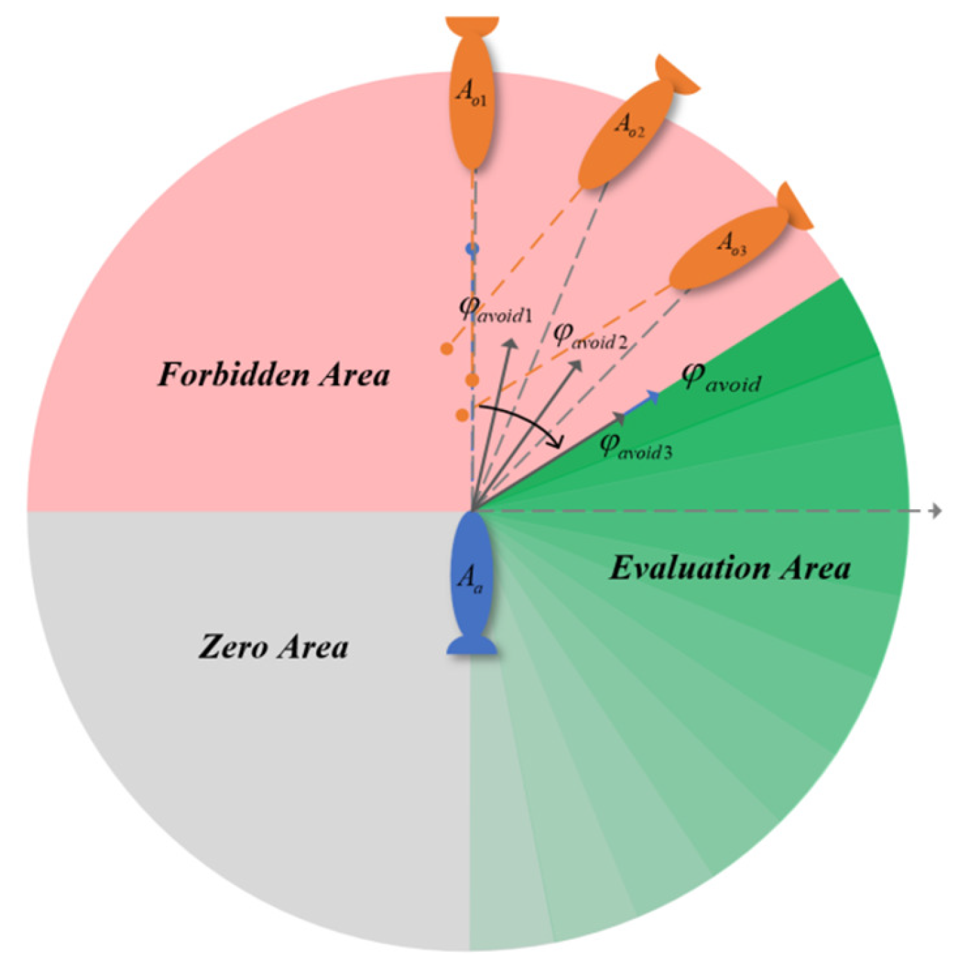
4.2. DWA Collision Avoidance Rule Evaluation Function

In this paper, we propose a collision avoidance rule in which an AUV needs to avoid to the right side, and, in Figure 7, A a takes the non-collision direction with a clockwise magnitude of Δ θ a v in the θ a o direction at this time as the base avoidance direction, which is calculated by the following equation:
φ n i = θ a o i Δ θ a v   ,   θ a o i Δ θ a v > π 2 π + θ a o i Δ θ a v   ,   θ a o i Δ θ a v π ( Δ θ a v π 4 )
In the equation, θ a o i is the direction of the i-th AUV to be avoided relative to the AUV A a , φ n i is the corresponding i-th avoidance direction, and Δ θ a v is the avoidance magnitude.
When A a needs to avoid multiple AUVs at the same time, a predetermined avoidance direction should be calculated for each potential collision target, from which the largest avoidance direction in the clockwise direction should be selected as the final avoidance direction, as shown in Figure 8. The calculation expression for the optimal avoidance direction is shown as follows:
φ o b = min ( min ( φ r b φ n 1 , 2 π φ r b φ n 1 ) , min ( φ r b φ n 2 , 2 π φ r b φ n 2 ) , , min ( φ r b φ n m , 2 π φ r b φ n m ) )
and
φ r b = φ a π ,   φ a 0 φ a ,   φ a < 0  
φ a is the bow angle of AUV A a .
The closer the end bow of the trajectory is to φ o b , the higher the evaluation value of the rule evaluation function is, and the expression of the rule evaluation function is as follows:
avoid ( v , ω ) = 2 π min ( φ a T τ φ o b , 2 π φ a T τ φ o b )
In the above equation, φ a T τ is the bow angle at the end of the predicted trajectory of the AUV of this side.

5. Distributed Dynamic Target Hunting by AUVs Based on CPPPEA

This section proposes the CPPPEA (Consensus-Based Polynomial Prediction and Polygonal Encirclement Algorithm), in which the consistency algorithm ensures the reliability of AUV cluster distributed cooperation, the polynomial regression algorithm predicts the trajectory of dynamic targets in real time, providing data support for encirclement, and the standard polygon strategy can achieve the generation of encirclement potential points and efficient encirclement of targets.

5.1. AUV Swarm Consistency Algorithm

We introduce a leader–follower architecture with a robust leader election mechanism to ensure information consistency and fault tolerance within the AUV swarm. The consistency algorithm ensures that even when the leader AUV fails, the cluster of capture tasks can maintain high availability and stability.
A distributed consistency scheme is designed based on BASE theory, as shown in Figure 9. In the distributed swarm, all nodes can be in one of three states: follower, candidate, or leader. The leader node is elected to handle and maintain the consistency of distributed information. The leader periodically sends heartbeat messages to synchronize information within the swarm and maintain its term. If the leader node fails, a new leader is elected, and the term number is incremented. If the previous leader recovers and receives heartbeat data with a higher term number from the new leader, it will automatically revert to the follower state. When selecting a new leader, candidates will first vote for themselves and send a message requesting voting to other nodes in the cluster. When a candidate node receives more than half of the votes, it will be promoted to a leader node, and its term will be increased by 1. This mechanism ensures the information consistency and high availability of the distributed system.

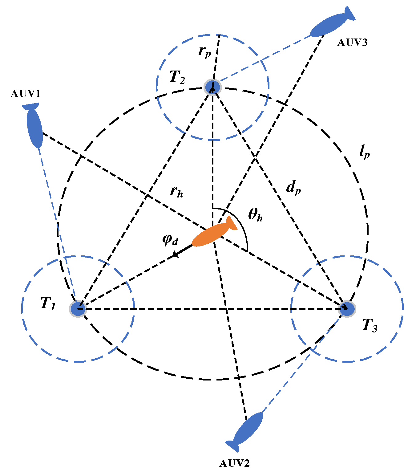
5.2. Formation Method of the Hunting Formation

We propose a novel hunting formation strategy that leverages target trajectory prediction and real-time AUV status to achieve efficient encirclement. This method includes the trajectory prediction of moving targets, the generation of capture base points, the and generation of capture potential points.

5.2.1. Nonlinear Regression Fitting of Moving Target Trajectories

The polynomial regression method is a flexible regression technique that models data by establishing a polynomial relationship between the independent and dependent variables [27]. For the trajectory of a moving target in the ocean over a period of time, the trajectory can be fitted using a univariate polynomial regression model with the following equation:
f ( x ) = β 0 + β 1 x + β 2 x 2 + β 3 x 3 + β n x n
In the equation, β is the coefficient of each term.
For the trajectory fitting of moving targets, the method of decoupling each coordinate by time step is used to reduce the number of polynomials in each dimension in order to improve the fitting accuracy, and the relationship between the target position and the time step can be obtained, which is defined in the model as follows:
x i = β 0 + β 1 t i + β 2 t i 2 + β 3 t i 3 + β n t i n
The model can be written as a system of linear equations since the dataset has multiple steps of data:
X = A β x s 1 x s 2 x s 3 x s n = 1 t 1 t 1 2 t 1 n 1 t 2 t 2 2 t 2 n 1 t 3 t 3 2 t 3 n 1 1 t m t m 2 t m n β 0 β 1 β 2 β n
The vector of polynomial regression coefficients estimated using least squares is as follows:
β ^ = ( A T A ) 1 A T X
Assuming that n < m is a necessary condition for matrix invertibility, then, since A is a Vandermont matrix, the invertibility condition is guaranteed to hold if all t i values are not the same, which is the only least squares solution.
In order to accelerate the speed of parameter convergence, the coordinates of the existing trajectory data are standardized as training data, and the mean σ and standard deviation μ of all coordinate values in the data are calculated and standardized according to the following equation:
x s i = x i μ σ
Let the prediction function be
f β ( t ) = β 0 + β 1 t + β 2 t 2 + β n t n
Then the objective function of the regression algorithm is as follows:
E ( β ) = 1 2 i = 1 m ( x s i f β ( t i ) ) 2
All parameters are updated in a synchronized loop to ensure that the gradient direction remains stable, and the parameter update expression is as follows:
β j ' = β j η i = 1 m ( f β ( t i ) x s i ) t i j
In the equation, η is the learning rate when the model parameters are updated.
The dataset is approximated by increasing the higher terms of the independent variables until the error is minimized, and, finally, the trajectory equation of the target position with respect to time is generated.

5.2.2. Calculation Method for Hunting Base Point

The hunting base point is defined as the location where the AUV swarm can encounter the moving target in the shortest time. After fitting the trajectory equation of the moving target using a regression method, the target’s motion trajectory is converted into a discrete set of points { P i } , with intervals corresponding to the AUV’s motion cycle τ . The task is to calculate the earliest point P k , where the AUV, starting from its current position X a and accelerating with maximum acceleration, can encounter the dynamic target. A decision variable d i is introduced to indicate whether the i-th point is selected as the encounter point. The problem can then be further formulated as finding the value of i that minimizes t i . The formula is as follows:
min   i = 1 n d i t i s . t .   i = 1 n d i = 1   and   t i t P i d i { 0 , 1 } , i
In the equation, t h is the time required for the AUV to reach point t P i .
The time for the AUV to reach the encounter point is mainly considered to calculate the displacement time t d and the steering time t φ .
The calculation of t d needs to consider the current position X a , current speed v a , maximum acceleration a , and maximum cruise speed v m of the AUV, which are calculated separately according to whether the maximum cruise speed can be reached during the voyage and are expressed as follows:
t d = 2 a P i X a 2 + ( v m v a ) 2 2 a v m , P i X a 2 > v m 2 v a 2 2 a t d = v a ± v a 2 + 2 a P i X a 2 a ,   otherwise   ( t d 0 )  
The calculation of t φ needs to consider the current bow angle φ a , current bow angular velocity ω a , maximum bow angular acceleration α , and maximum bow angular velocity ω m of the AUV, which are calculated according to whether the maximum bow angular velocity can be reached or not during steering, and their expressions are as follows:
t φ = ω m ω a + ω m α + φ p i φ a φ m ω m ,   φ p i φ a > φ m t φ = ω m i d ω a + ω m i d α ,   otherwise   ( t φ 0 )
φ m = 2 ω m 2 + s ω a 2 2
ω m i d = 2 α φ p i φ a + s ω a 2 2
In the equation, φ m is the total change of bow direction during acceleration from the current bow angular velocity to the maximum bow angular velocity and deceleration from the maximum bow angular velocity to 0; ω m i d is the intermediate bow angular velocity, if it is not possible to reach the maximum bow angular velocity during steering, deceleration is made ω m i d when it is reached, and the bow is facing φ p i when deceleration is made to 0; s is the sign factor.
The time t P i to reach point P i can be approximated as follows:
t P i = max ( t d , t φ )
The above calculation yields the set of fastest encounter points { p K j } between each AUV and a moving target and the fastest encounter time t K j between each AUV and a moving target. Then the slowest encounter point P h is the roundup base point of the AUV cluster.

5.2.3. Moving Target Hunting Formation Method

Collaborative roundup by AUVs aims to construct a polygonal roundup formation centered on the roundup target and formed by the participating AUVs to surround the target. The leader AUV, elected by the coherence algorithm, acts as the roundup planning organizer and is responsible for planning the potential points of other follower AUVs when rounding up the moving target. The method for determining the roundup potential point is demonstrated in Figure 10.
Based on the standard polygon strategy to generate the roundup potential points, the previously calculated roundup base point P h ( x h , y h ) is used as the polar coordinate origin, the potential points are assigned on the roundup encirclement circle with radius r h , and the angle between neighboring roundup potential points is θ h = 2 π / m . T i ( x T i , y T i ) ( i = 1 , 2 , , m ) is the potential points around the rounded up target, the set of roundup potential points is T = { T 1 , T 2 , , T n } ( i = 1 , 2 , , m ) , and the formula for roundup point coordinates is as follows:
x T i = x h + r h cos ( φ d + ( i 1 ) 2 π m ) y T i = y h + r h sin ( φ d + ( i 1 ) 2 π m )
In the above equation, φ d is the heading of the moving target when it moves to the roundup base P h , and m is the number of AUVs participating in the roundup mission.
To achieve optimal allocation of capture potential points for each AUV, the motion direction of the moving target is taken as the polar-axis 0-degrees direction, and clockwise direction is taken as the positive direction. Calculate the polar angle θ a i of each AUV’s current position. Then, sort each AUV in ascending order of the polar angle to obtain set A = A 1 , A 2 , A 3 , , A i i = 1 , 2 , , m . Correspond the elements in sets A and T one by one in order, and the T i element corresponding to each AUV is the encirclement potential point that the AUV needs to reach.
The maximum radius of the rounding potential point is r p , the maximum radius of the target to be rounded up is r d , the safety distance between AUVs is set to d s , and conditions d s > r p , d s > r d need to be set in order to ensure the safety of the rounding up task in which the radius of the rounding potential point r p and the arc length between neighboring potential points l p need to meet the following requirements:
2 r p + β 1 d s l p r d + r p + β 2 d s r h ( β 1 , β 2 1 )
β 1 and β 2 are safe distance factors.
Due to the constraint of arc length l p , the distance between the AUVs and the moving target will limit the size of the roundup radius so the number of AUVs participating in the roundup will be limited. Assuming that there are m AUVs, the roundup radius is m l p = 2 π d h , and solving for the minimum roundup radius based on the conditions of the above inequality yields the relationship between the number of AUVs and each parameter as follows:
m = 2 π ( r p + r d + β 2 d s ) 2 r p + β 1 d s
When the AUV clusters enter the state of predetermined conversion to a roundup formation, they will move toward their respective designated roundup potential points to form an effective roundup formation, as shown in Figure 11.

6. Simulation Results

In order to validate the proposed method and its adaptability and efficiency under different conditions, a series of simulation experiments are carried out to set up a total of five AUVs within the mission range of 500 m × 500 m to participate in the encirclement mission and to encircle the moving target as an enemy AUV. The moving target is driven to the target point before this if the AUV cluster forms the formation of encirclement, and then encirclement will be successful, or else it is regarded as a failure of the encirclement.

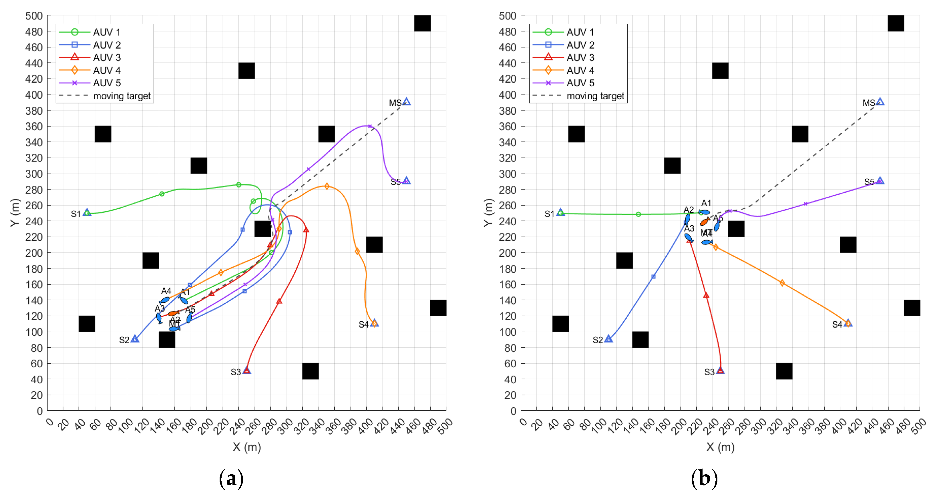
6.1. Simulation of Target Hunting Task When the Moving Target’s Speed Is Less than the AUV’s

In conventional hunting methods, a prerequisite for successful hunting is that the hunter’s (AUV’s) speed must be greater than that of the target. If this condition is not met, the success rate of the hunting task will be significantly reduced. To address this issue, this section presents a simulation experiment aimed at comparing the effectiveness of the traditional tracking hunting method with the hunting method proposed in this paper for capturing a moving target in an environment with obstacles. The initial states of the AUV and the moving target in the experiment are detailed in Table 1.
The simulation results are shown in Figure 12, visually illustrating the differences in the motion trajectories between the traditional tracking hunting method and the hunting method proposed in this paper. The proposed method performs excellently in reducing redundant travel paths and is able to form an effective hunting formation more quickly. Through the quantitative analysis of the simulation data, and, in conjunction with the results in Table 2, it is evident that the proposed method significantly outperforms the traditional tracking hunting method in key performance indicators such as travel distanceand turning angle cost.

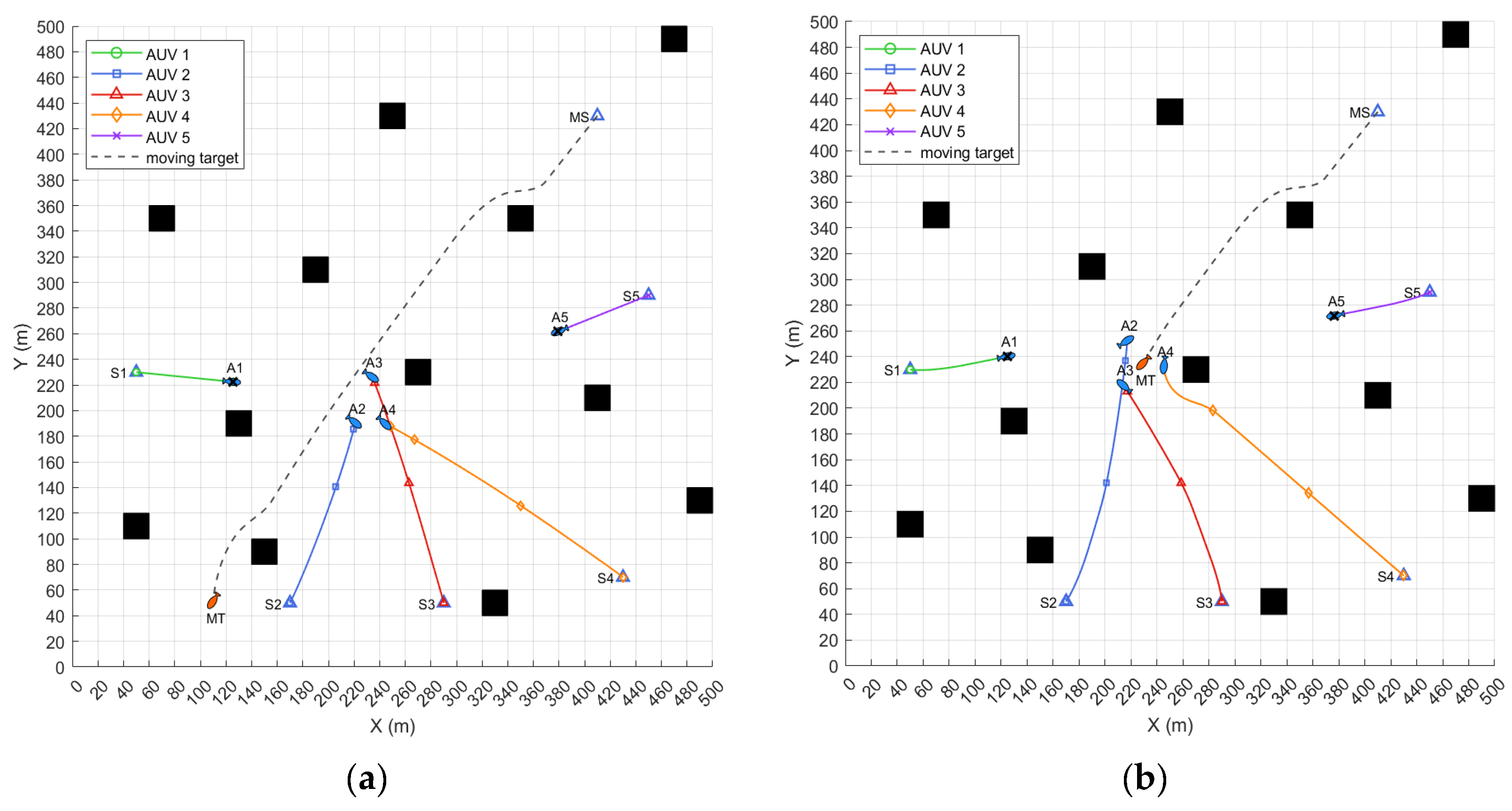
6.2. Simulation of the Hunting Task When the Moving Target’s Speed Equals the AUV’s

This section tests the adaptability and effectiveness of the proposed hunting method under the challenge of equal speeds, breaking the traditional condition where the hunter’s speed exceeds that of the target. The test is conducted under the scenario where the moving target’s speed equals the AUV’s speed. This setup aims to explore the performance of the traditional tracking hunting method and the proposed hunting method when the hunting AUV has no speed advantage. The initial states of the AUV and the moving target in the experiment are detailed in Table 3.
The simulation results, as shown in Figure 13, demonstrate the challenges faced by the traditional tracking hunting method under the condition where the hunting AUV and the moving target have the same speed. Specifically, when the AUV needs to perform maneuvering and obstacle avoidance, it is unable to catch up with the moving target again, preventing the formation of an effective hunting formation and ultimately leading to a failure of the hunting task. In contrast, the method proposed in this paper breaks the traditional limitation that the hunter’s speed must be greater than that of the target. By pre-planning hunting positions and adjusting strategies in real time, it effectively overcomes the hunting challenge under equal speed conditions. Based on the analysis of various indicators in Table 4, the key to the success of the proposed algorithm in executing the hunting task lies in its ability to rapidly form an effective hunting formation with relatively low motion and adjustment costs.

6.3. Simulation of Hunting Task When the Leader Fails

To test the availability of the consistency algorithm proposed in this paper when facing leader failure, this section simulates the failure of the leader AUV and a randomly selected AUV during the hunting process, causing them to be unable to maintain the original course. Additionally, a scenario where the moving target’s speed equals the AUV’s speed is set up for testing. The aim is to evaluate the usability of the proposed hunting method under the complex condition of no speed advantage and leader failure. The initial setup for the experiment is detailed in Table 5.
As shown in Figure 14a, the hunting task swarm that does not use the consistency algorithm proposed in this paper faces difficulty in effectively updating decisions and synchronizing information after the leader node fails. As a result, the swarm can only continue the hunting task based on the potential point allocation before the failure. Unable to adjust in time to match the actual trajectory of the moving target and failing to form an effective hunting formation, this situation ultimately leads to the failure of the hunting task. In contrast, as shown in Figure 14b, the hunting task swarm that applies the consistency algorithm proposed in this paper is able to adapt to changes by re-electing a leader and making task decisions after the leader node fails. By setting up a reformation strategy for the AUVs in normal operation and reallocating the hunting potential points, the continuity of the task is ensured. Ultimately, three functioning AUVs cooperatively completed the effective interception of the target and the formation of the hunting formation. Based on the analysis of the various indicators in Table 6, the proposed algorithm can ensure the completion of the hunting task even when a few AUVs experience failures.

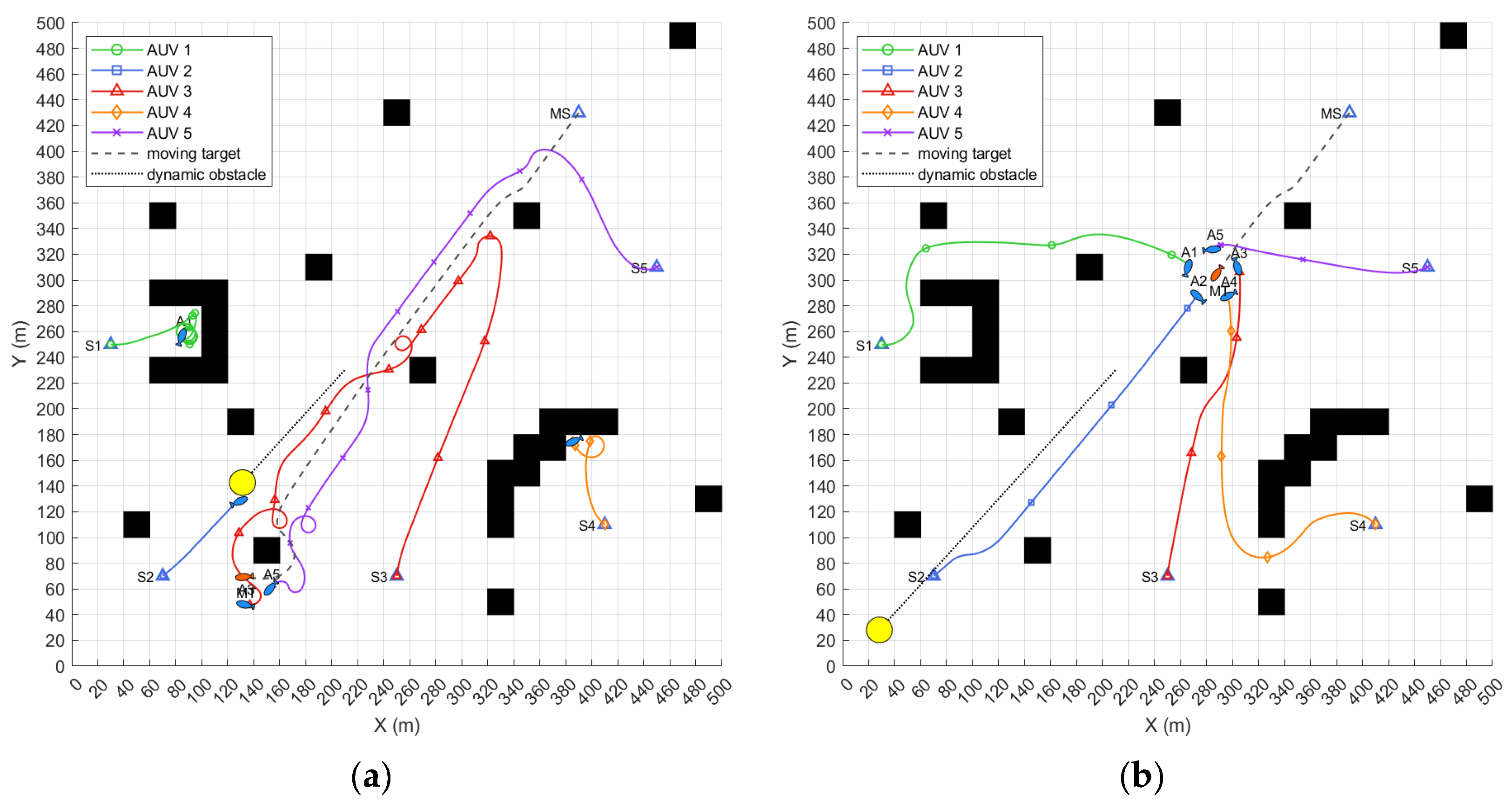
6.4. Simulation of Hunting Task in a Complex Obstacle Environment

In this section’s hunting experiment, an environment with concave obstacles, dynamic obstacles, and trap areas is set up to comprehensively test the effectiveness of the motion planning algorithm and hunting method proposed in this paper. The initial setup for the experiment is detailed in Table 7.
The simulation results, as shown in Figure 15, demonstrate that when the AUVs use the traditional DWA for hunting motion planning, they face several challenges. Due to the lack of foresight, AUV1 and AUV4 become trapped in local areas when encountering concave obstacles with trap zones, while AUV2, with a relatively high relative speed, is unable to avoid a dynamic obstacle in time, resulting in a collision. As a result, the number of remaining AUVs capable of completing the hunting task is insufficient to form an effective hunting formation. In contrast, the motion planning algorithm based on the improved DWA proposed in this paper is able to bypass local obstacle areas and avoid dynamic obstacles in time. After obstacle avoidance, the algorithm adjusts the strategy in real time, ensuring that all AUVs successfully avoid obstacles and can form an effective hunting formation. Based on the analysis of the various indicators in Table 8, the proposed algorithm can accomplish the hunting task in environments with complex static and dynamic obstacles.

7. Conclusions

This paper investigates the dynamic target hunting problem under AUV motion planning based on the improved DWA. Firstly, by optimizing the speed space and evaluation function of the DWA algorithm and incorporating an obstacle detection window and integrating SAGRRT planning for static obstacle guidance points, the issue of DWA stagnating due to the evaluation value falling into local optima is effectively addressed. At the same time, after establishing a collision risk zone, dynamic obstacle avoidance guidance points are planned through DAGRRT to guide the DWA motion planning, enabling dynamic obstacle avoidance.
Secondly, a dynamic collision avoidance algorithm based on consistency collision avoidance rules is proposed, and the collision avoidance rules are integrated into the DWA evaluation system. The rule evaluation function is used to select motion trajectories that comply with the collision avoidance rules, significantly improving the safety and efficiency of distributed AUV collision avoidance.
Next, a consistency algorithm is introduced to ensure the consistency of multi-AUV information and the continuity of tasks in the case of leader failure. Polynomial regression is used to predict the moving target’s trajectory, hunting potential points are dynamically allocated based on a polygonal hunting formation, and each AUV’s distributed motion planning is combined to form the hunting formation.
Finally, simulations verify that this series of systematic methods can effectively enhance the usability and efficiency of multi-AUV distributed dynamic target hunting. In fact, underwater communication issues have a significant impact on AUV collaborative operations, and this aspect should be considered in future research.

Author Contributions

Conceptualization, J.L. and H.L.; methodology, J.L.; software, J.L.; validation, J.L. and H.L.; formal analysis, J.L.; investigation, J.L. and H.L.; resources, J.L.; data curation, H.Z.; writing—original draft preparation, J.L.; writing—review and editing, Z.Z. and H.L.; visualization, H.Z. and H.L.; supervision, J.L.; project administration, J.L.; funding acquisition, J.L. All authors have read and agreed to the published version of the manuscript.

Funding

This search work was supported by the National Natural Science Foundation of China (Grant No. 5217110503), the Research Fund from Science and Technology on Underwater Vehicle Technology (grant No. JCKYS2021SXJQR-09), and the Natural Science Foundation of Shandong Province (grant No. ZR202103070036).

Institutional Review Board Statement

Not applicable.

Informed Consent Statement

Not applicable.

Data Availability Statement

Data are contained within the article.

Conflicts of Interest

The authors declare no conflicts of interest.

References

  1. Wang, L.; Zhu, D.; Pang, W.; Zhang, Y. A survey of underwater search for multi-target using Multi-AUV: Task allocation, path planning, and formation control. Ocean. Eng. 2023, 278, 114393. [Google Scholar] [CrossRef]
  2. Cheng, C.; Sha, Q.; He, B.; Li, G. Path planning and obstacle avoidance for AUV: A review. Ocean. Eng. 2021, 235, 109355. [Google Scholar] [CrossRef]
  3. Hao, K.; Zhao, J.; Li, Z.; Liu, Y.; Zhao, L. Dynamic path planning of a three-dimensional underwater AUV based on an adaptive genetic algorithm. Ocean. Eng. 2022, 263, 112421. [Google Scholar] [CrossRef]
  4. Xiang, X.; Yu, C.; Zhang, Q. On intelligent risk analysis and critical decision of underwater robotic vehicle. Ocean. Eng. 2017, 140, 453–465. [Google Scholar] [CrossRef]
  5. Zhang, W.; Wang, N.; Wu, W. A hybrid path planning algorithm considering AUV dynamic constraints based on improved A* algorithm and APF algorithm. Ocean. Eng. 2023, 285, 115333. [Google Scholar] [CrossRef]
  6. Liu, T.; Zhao, J.; Huang, J.; Li, Z. A hybrid RVO-MPPI approach for efficient collision avoidance for multiple autonomous underwater vehicles. Ocean. Eng. 2024, 312, 119205. [Google Scholar] [CrossRef]
  7. Zhang, J.; Zhu, Z.; Xue, Y.; Deng, Z.; Qin, H. Local path planning of under-actuated AUV based on VADWA considering dynamic model. Ocean. Eng. 2024, 310, 118705. [Google Scholar] [CrossRef]
  8. Rösmann, C.; Feiten, W.; Wösch, T.; Hoffmann, F.; Bertram, T. Trajectory modification considering dynamic constraints of autonomous robots. In Proceedings of the ROBOTIK 2012—7th German Conference on Robotics, Munich, Germany, 22–25 May 2012; pp. 74–79. [Google Scholar]
  9. Guo, Y.; Liu, H.; Fan, X.; Lyu, W. Research progress of path planning methods for autonomous underwater vehicle. Math. Probl. Eng. 2021, 2021, 8847863. [Google Scholar] [CrossRef]
  10. Molinos, E.J.; Llamazares, A.; Ocaña, M. Dynamic window based approaches for avoiding obstacles in moving. Robot. Auton. Syst. 2019, 118, 112–130. [Google Scholar] [CrossRef]
  11. Liu, Y.; Wang, C.; Wu, H.; Wei, Y. Mobile Robot Path Planning Based on Kinematically Constrained A-Star Algorithm and DWA Fusion Algorithm. Mathematics 2023, 11, 4552. [Google Scholar] [CrossRef]
  12. Song, B.; Tang, S.; Li, Y. A new path planning strategy integrating improved ACO and DWA algorithms for mobile robots in dynamic environments. Math. Biosci. Eng. MBE 2024, 21, 2189–2211. [Google Scholar] [CrossRef] [PubMed]
  13. Xu, T. Recent advances in Rapidly-exploring random tree: A review. Heliyon 2024, 10, e32451. [Google Scholar] [CrossRef] [PubMed]
  14. Hu, W.; Chen, S.; Liu, Z.; Luo, X.; Xu, J. HA-RRT: A heuristic and adaptive RRT algorithm for ship path planning. Ocean. Eng. 2024, 316, 119906. [Google Scholar] [CrossRef]
  15. Li, J.; Zhang, Z. AUV Local Path Planning Based on Fusion of Improved DWA and RRT Algorithms. In Proceedings of the ICMA 2023—2023 IEEE International Conference on Mechatronics and Automation, Harbin, China, 6–9 August 2023; pp. 935–941. [Google Scholar]
  16. Zhu, Y.; Liu, J.; Guo, C.; Song, P.; Zhang, J.; Zhu, J. Prediction of Battlefield Target Trajectory Based on LSTM. In Proceedings of the ICCA 2020 IEEE International Conference on Control and Automation, Singapore, 9–11 October 2020; pp. 725–730. [Google Scholar]
  17. Wang, H.; Wang, X.; Yu, L.; Zhong, F. Design of Mean Shift Tracking Algorithm Based on Target Position Prediction. In Proceedings of the ICMA 2019—2019 IEEE International Conference on Mechatronics and Automation, Tianjin, China, 4–7 August 2019; pp. 1114–1119. [Google Scholar]
  18. Zhang, R.; Wang, Y.; Wan, X.; Ming, Y.; Yang, S. Position prediction of underwater gliders based on a new heterogeneous model ensemble method. Ocean. Eng. 2024, 309, 118312. [Google Scholar] [CrossRef]
  19. Meng, X.; Sun, B.; Zhu, D. Harbour protection: Moving invasion target interception for multi-AUV based on prediction planning interception method. Ocean. Eng. 2021, 219, 108268. [Google Scholar] [CrossRef]
  20. Lan, Y. Multiple mobile robot cooperative target intercept with local coordination. In Proceedings of the CCDC 2012—2012 24th Chinese Control and Decision Conference, Taiyuan, China, 23–25 May 2012; pp. 145–151. [Google Scholar]
  21. Tahir, M.N.; Ren, Z. Maneuvering target interception using retrospective-cost-based adaptive input and state estimation. In Proceedings of the CGNCC 2016—2016 IEEE Chinese Guidance, Navigation and Control Conference, Nanjing, China, 12–14 August 2016; pp. 603–608. [Google Scholar]
  22. Refsnes, J.E.; Sorensen, A.J.; Pettersen, K.Y. Model-based output feedback control of slender-body underactuated AUVs: Theory and experiments. IEEE Trans. Control. Syst. Technol. 2008, 16, 930–946. [Google Scholar] [CrossRef]
  23. Cao, X.; Sun, H.; Jan, G.E. Multi-AUV cooperative target search and tracking in unknown underwater environment. Ocean. Eng. 2018, 150, 1–11. [Google Scholar] [CrossRef]
  24. Han, L.; Wu, X.; Sun, X. Hybrid path planning algorithm for mobile robot based on A* algorithm fused with DWA. In Proceedings of the ICIBA 2023—2023 IEEE 3rd International Conference on Information Technology, Big Data and Artificial Intelligence, Chongqing, China, 26–28 May 2023; pp. 1465–1469. [Google Scholar]
  25. Wu, B.; Chi, X.; Zhao, C.; Zhang, W.; Lu, Y.; Jiang, D. Dynamic Path Planning for Forklift AGV Based on Smoothing A* and Improved DWA Hybrid Algorithm. Sensors 2022, 22, 7079. [Google Scholar] [CrossRef] [PubMed]
  26. Zhong, X.; Tian, J.; Hu, H.; Peng, X. Hybrid Path Planning Based on Safe A* Algorithm and Adaptive Window Approach for Mobile Robot in Large-Scale Dynamic Environment. J. Intell. Robot. Syst. Theory Appl. 2020, 99, 65–77. [Google Scholar] [CrossRef]
  27. Yu, Q.; Lin, Q.; Zhu, Z.; Wong, K.C.; Coello, C.A. A dynamic multi-objective evolutionary algorithm based on polynomial regression and adaptive clustering. Swarm Evol. Comput. 2022, 71, 101075. [Google Scholar] [CrossRef]
Figure 1. Sonar sensor model.
Jmse 13 00221 g001
Figure 2. Obstacle sampling window.
Jmse 13 00221 g002
Figure 3. Global target points linearly connected nodes as SAGRRT local target points.
Jmse 13 00221 g003
Figure 4. Extract key guiding points.
Jmse 13 00221 g004
Figure 5. Introduction of DAGRRT dynamic obstacle avoidance.
Jmse 13 00221 g005
Figure 6. Bump avoidance space division.
Jmse 13 00221 g006
Figure 7. Baseline avoidance directions and evaluation intervals.
Jmse 13 00221 g007
Figure 8. Multi-avoidance condition baseline avoidance direction and evaluation interval.
Jmse 13 00221 g008
Figure 9. Consistency algorithm.
Jmse 13 00221 g009
Figure 10. Distribution of the potential points in the hunting process.
Jmse 13 00221 g010
Figure 11. Diagram of hunting formation and maintenance.
Jmse 13 00221 g011
Figure 12. (a) Simulation of tracking hunting method when the moving target’s speed is less than the AUV’s; (b) simulation of tracking hunting method when the moving target’s speed is less than the AUV’s.
Jmse 13 00221 g012
Figure 13. (a) Simulation of tracking hunting method when the moving target’s speed equals the AUV’s; (b) simulation of the hunting method proposed in this paper when the moving target’s speed equals the AUV’s.
Jmse 13 00221 g013
Figure 14. (a) Simulation of hunting without using the consistency algorithm when a failure occurs; (b) simulation of hunting using the consistency algorithm proposed in this paper when a failure occurs.
Jmse 13 00221 g014
Figure 15. (a) Simulation of hunting motion planning using traditional DWA; (b) simulation of hunting motion planning using traditional DWA.
Jmse 13 00221 g015
Table 1. Initial state of AUV and moving target.
Mission
Elements
Initial
Position/m
Bow Angle
/rad
Initial Speed
/kn
Maximum Speed/kn
AUV150,250−0.104
AUV211,0900.704
AUV325,0501.504
AUV4410,1102.404
AUV5450,290−2.804
Moving target450,390−2.502
Table 2. Simulation results of hunting motion planning when the moving target’s speed is less than the AUV’s.
Hunting MethodHunting SuccessTravel Distance/mTurning Cost/rad
Tracking huntingYes1692.3126.7
The proposed methodYes1123.836.1
Table 3. Initial state of AUV and moving target.
Mission
Elements
Initial
Position/m
Bow Angle
/rad
Initial Speed
/kn
Maximum Speed/kn
AUV150,250−0.104
AUV211,0900.704
AUV325,0501.504
AUV4410,1102.404
AUV5450,290−2.804
Moving target450,390−2.504
Table 4. Simulation results of hunting motion planning when the moving target’s speed equals the AUV’s.
Hunting MethodHunting SuccessTravel Distance/mTurning Cost/rad
Tracking huntingNo2088.563.9
The proposed methodYes976.644.7
Table 5. Initial state of AUV and moving target.
Mission
Elements
Initial
Position/m
Bow Angle
/rad
Initial Speed
/kn
Maximum Speed/kn
AUV150,230004
AUV217,0501.104
AUV329,0501.704
AUV443,0702.404
AUV5450,290−2.804
Moving target410,230−2.204
Table 6. Simulation results of hunting motion planning when a failure occurs.
Hunting MethodHunting SuccessTravel Distance/mTurning Cost/rad
Tracking huntingNo707.620.5
The proposed methodYes796.622.8
Table 7. Initial states of the AUV, moving target, and dynamic obstacle.
Mission
Elements
Initial
Position/m
Bow Angle
/rad
Initial Speed
/kn
Maximum Speed/kn
AUV130,250−0.104
AUV270700.704
AUV325,0701.404
AUV4410,1102.404
AUV5450,310−2.704
Moving target390,430−2.202
Dynamic obstacle210,230−2.31111
Table 8. Simulation results of hunting motion planning in a complex obstacle environment.
Hunting MethodHunting SuccessTravel Distance/mTurning Cost/rad
DWA + tracking huntingNo1835.9178.9
The proposed methodYes1346.244.3
Disclaimer/Publisher’s Note: The statements, opinions and data contained in all publications are solely those of the individual author(s) and contributor(s) and not of MDPI and/or the editor(s). MDPI and/or the editor(s) disclaim responsibility for any injury to people or property resulting from any ideas, methods, instructions or products referred to in the content.

