Novel Method for Predicting Linear Velocity Derivative in Modern Ship Hulls and Its Validation Using a Low-Speed Maneuvering Simulator

Abstract

Ship maneuvering prediction relies on hydrodynamic derivatives, traditionally obtained through empirical formulations based on hulls built decades ago. A comparison with experimental data revealed a notable discrepancy, particularly for the linear sway velocity derivative ($Y_V^{\prime }$), where these regression models inadequately capture the behavior of modern hulls. To overcome this limitation, a novel approach is proposed, in which 690 virtual static drift tests were conducted across a systematic series of 115 modern hull forms, parametrically generated in the Grasshopper platform and thus benchmarked against seven vessels. This extensive numerical dataset enabled the development of an updated regression formulation for $Y_V^{\prime }$, which was grounded in key geometric parameters and incorporated specific terms related to the bow and stern shapes. The results obtained by the CFD-based method were compared with those obtained experimentally, confirming the high fidelity of this approach, yielding a maximum relative error of only $\mathbf{4.7}\%$ for the sway linear velocity derivative. Crucially, when this proposed empirical formula was integrated into a mathematical model (MM-TPN) to predict a ship’s trajectory, it demonstrated substantial improvement by reducing the absolute relative error in standard maneuvers from $\mathbf{23}\%$ to $\mathbf{10}\%$ compared with traditional methods used to describe the $Y_V^{\prime }$. Furthermore, an extensive discussion regarding the regression model was conducted, leading to the establishment of the drift angle threshold that invalidates the linear theory (set at ${\mathbf{10}}^{\circ }$ for blunt hulls and ${\mathbf{8}}^{\circ }$ for slender hulls). A comprehensive three-step validation process, encompassing the $V\&V$ of the virtual static drift tests, validation of the derived maneuvering coefficient, and validation through standard maneuvers employing the novel approach proposed here, was fully executed.

1. Introduction

Modern hulls have sophisticated lines that shape them to enhance their resistance performance and reduce fuel consumption, aligning with the increasing focus on environmental concerns and regulations. An example is the International Maritime Organization (IMO), which introduced regulations on energy efficiency, known as the Energy Efficiency Design Index (EEDI), which became mandatory from 2013 onwards and has pushed change in ship design. Ref. [1] highlighted a concern that meeting the EEDI requirements might lead to a reduction in installed power, potentially impacting the ship’s maneuverability and operational safety. Furthermore, modern design features such as bulbous bows, stern transoms, and increased size challenge the validity of traditional maneuvering predictions based on regression analysis.

Ship maneuverability, an intrinsic hull characteristic, is assessed by the vessel’s ability to perform actions such as turning and course-keeping, typically evaluated in accordance with IMO Resolution MSC 137(76) [2]; which all ships larger than 100 m of L_PP or any chemical vessel must follow. The prevailing methodology for predicting ship motion involves mathematical models that require maneuvering coefficients (derivatives) to describe the hydrodynamic counterpart. Historically, the preferred strategy for determining these derivatives has relied on empirical formulations derived from captive model tests, such as planar motion mechanism (PMM) and rotating arm tests. Although accurate, experiment-based models are costly and limited by geometry, i.e., modifying the hull geometry or even altering the draft can be challenging and expensive. In 1993, an extensive manual on maneuvering was published [3], and the author emphasized the inadequacy of crude estimates based on hull dimensions for describing a ship’s maneuvering characteristics. He also highlighted how fast the ships are increasing, and as a consequence, the empirical methods previously used to predict the forces acting on the hull no longer reflect modern design realities.

Indeed, traditional empirical predictions for the linear sway velocity derivative ($Y_V^{\prime }$) exhibit significant discrepancies relative to experimental data for modern vessels. Specifically, current formulations often overestimate $Y_V^{\prime }$ for modern slender hulls with bulbous bows. Moving beyond the limitations of the empirical formulation, the current focus shifts to developing a tool that efficiently and accurately determines these coefficients. A new method attracting attention in this field is the virtual captive model test, which has gained traction in many practical applications due to its flexibility and low cost of implementing different hull shapes and flow conditions. However, in the literature, it remains unclear how to perform such tests while increasing the drift angle. This challenge arises because the $Y_V^{\prime }$ are fundamentally derived from linear theory; however, on the hydrodynamic side, non-linear behavior is expected to manifest once flow separation occurs, but the threshold angle has not yet been established.

Building upon the preceding discussion, two fundamental questions remain and guide the subsequent methodology. Initially, the threshold for the drift angle that limits the validity of the linear theory must be established. Secondly, the adequacy of the traditional regression formulation for determining the linear velocity derivative ($Y_V^{\prime }$) for modern hull forms must be critically assessed. To address these points, a three-step validation process is proposed herein: the $V\&V$ of the virtual static drift tests, a validation of the linear derivatives themselves, followed by a validation through standard maneuvers performed in fast-time simulations using the Numerical Offshore Tank Mathematical Model (MM-TPN). This approach aimed to yield a robust numerical model for acquiring vessel-specific hydrodynamic coefficients and, subsequently, to create a reliable empirical formulation for $Y_V^{\prime }$ in scenarios where virtual testing is impractical.

The subsequent section of this article first present a chronological literature review of maneuver prediction and hydrodynamic coefficients, introducing the mathematical model and the theory of linear derivatives in Section 2. In Section 3, the $V\&V$ of the virtual static drift tests is given. Attention then shifts to understanding the prediction of maneuvering coefficients and establishing the threshold angle, where the linearity assumption is exhaustively discussed from both statistical and hydrodynamic perspectives in Section 4. Finally, the article presents the new approach to predicting the linear derivative in Section 5, utilizing the regression model derived from the systematic hull series generated primarily for this research.

2. State of the Art

2.1. Ship Maneuvering Prediction

The development of transport machines over the centuries has been guided by two immutable goals: the necessity of motion through a fluid medium (air or water) and the requirement to transfer control of the route to a human operator. Even the domestication of animals as primitive transport was driven by the desire to manage direction, as the fundamental purpose of transport is the guided transit of people or goods to a specific location. This inherent quality, which defines how easily a transport machine can be directed, is known as maneuverability, and this requirement is pursued in the design of a simple boat or an autonomous vessel. According to the French vocabulary, the word maneuverability of a ship covers all possible steady motions it may assume [4]. It is important to note that these words have two different spellings: maneuverability/maneuver or manoeuvrability/manoeuvre. The British and Canadian English prefer the latter, while the American English prefers the former. According to Google N-gram Viewer, a tool comprising over five hundred billion words from various books and monographs found in the Google Books database, the term maneuverability was found to be the most frequently used spelling in 2019, with a usage rate of $110\%$ higher than the British version. Thus, maneuverability/maneuver will be adopted in this text. In the Cambridge English Dictionary, this term is defined as the quality of being easy to move and direct. In the naval context, ship maneuverability studies deal with the motion of a rigid body on the surface of a real fluid, considering the effect of the body’s control surfaces. The invention of the rudder during the Middle Ages was pivotal, moving beyond oars to provide centralized control over steering. This control surface introduced two primary roles: altering the heading as desired and correcting deviations caused by flow disturbances around the hull. Besides its relevance, formal theoretical study of ship control began with Euler’s discoveries in the eighteenth century, as noted by [5]. However, it were [6] who first successfully unified the practical and theoretical aspects of ship dynamics relating to turning and course-keeping. Their work is considered a milestone in the ship performance field [7], establishing the foundation for evaluating steering, which they defined as the ship’s response when the rudder is maneuvered to achieve a specified position [6].

Recognizing the growing importance of the subject, the International Towing Tank Conference (ITTC) established a dedicated Maneuvering Committee in 1960. Back then, most maneuvering characteristics were assessed through free-running trials conducted at model scale in dedicated facilities; however, these trials are susceptible to scale effects. This susceptibility stems from the disproportionately dominant viscosity contribution at model-scale Reynolds numbers, which leads to an overestimation of propeller loading and misleading rudder forces, thereby compromising stability analyses. To address this scaling challenge, novel approaches emerged in the mid-1960s. The captive model test methodology, as highlighted by [8], provided a better scaling approach by breaking the problem into groups of hydrodynamic coefficients. Such an approach enabled independent extrapolation of each coefficient to full scale, thereby improving understanding of scale effects when combined with a mathematical model. This approach also leveraged theories such as the low-aspect-ratio wing theory, suggesting that the scale effect on the lateral force at small incidence angles would be minor [9].

During the ITTC’66, ref. [10] introduced two parameters to assess a ship’s steering quality. The paper referred to these parameters as the ratio of a steady turning angular rate (K) and a time parameter (T). The purpose of these indices was to provide a means of measuring a ship’s response to rudder actuation. The authors suggested that these steering quality indices could be derived from experimental free-running tests of prescribed trajectories, such as turning and zigzag tests. Concurrently, Winnifred R. Jacobs proposed an analytical method for ship stability analysis [11]. Her work established a critical stability relation that a stable ship must obey:

$${\displaystyle \frac{N_r^{\prime }}{Y_r^{\prime }-m^{\prime }}}>{\displaystyle \frac{N_v^{\prime }}{Y_v^{\prime }}}.$$

(1)

Jacobs introduced the idea of stability derivatives based on potential theory and low-aspect-ratio wing theory, thereby incorporating viscosity effects. A subsequent journal publication [12] provided a comprehensive comparison between her analytical method and experimental data, successfully confirming the effectiveness of the proposed method.

The increasing size of vessels, particularly tankers, and consequent accidents in restricted areas, as highlighted by [13] at the 11th ITTC, underscored the urgent need to understand transient and low-speed conditions. Motora detailed the critical loss of rudder efficiency and controllability during berthing maneuvers when the propeller is stopped or reversed, noting that maneuverability was often neglected in ship design despite its relevance to safety [14]. This safety imperative drove the development of comprehensive mathematical models. The foundational work by Abkowitz [9] utilized a Taylor series expansion for the integrated hull–propeller–rudder system. While initially focused on small angles at cruising speeds, ref. [15,16] adapted the model for low-speed, high-angle scenarios by introducing quadratic (nonlinear) approximations to account for viscous effects, which in turn required facilities like PMM to measure these new nonlinear terms [17]. Usually, these tests are performed in a towing tank, ref. [18] proposed an alternative approach, using a Circulating Water Channel (CWC) to obtain the maneuvering hydrodynamic derivatives. While the method proved reliable, with a statistical convergence error of less than $1\%$, this test is inherently limited by the facility dimension, consequently requiring a small-scale model. The authors extensively discussed the experimental uncertainty and its assessment on both approaches. Concurrently, the Japanese MMG (Manoeuvring Modeling Group) proposed a more flexible 3-DOF approach in the 1970s, separating the force contributions [19], which was later extended by [20] to include roll. Despite differing derivations, both models rely fundamentally on hydrodynamic derivatives.

Therefore, obtaining the hydrodynamic derivatives is a key factor, a task recognized by the International Towing Tank Conference (ITTC) as challenging [21]. Historically, the hydrodynamic coefficients required by these models were obtained through experimental tests. Ref. [22] noted the growth in experimental facilities, particularly in post-war Japan. Ref. [14] pointed out that as late as the 1990s, most simulator coefficients were still sourced from expensive and complex fully appended captive model tests (e.g., PMM, SDT), which demand large facilities to mitigate blockage issues. Several alternative methods emerged to overcome these challenges. In the late 1970s, system identification [23] was developed to estimate all coefficients simultaneously from free-running maneuver trajectories, thereby capturing interaction effects. From the 2000s onward, CFD has been widely used to compute the hydrodynamic forces and moments acting on ships, including the complex case of static drift tests at high angles, where flow separation may occur. Toxopeus [24] conducted an extensive study on verification and validation of the viscous flow computations at different drift angles and hull shapes. The author found promising results in both lateral force, yaw moment, and maneuvering prediction employing hydrodynamic coefficients obtained numerically, which brought some exciting aspects of using CFD to deal with maneuvering ship problems, focusing on the virtual captive model test.

Considering future solutions on ship maneuvers subject and emphasizing that the automation of berthing can significantly enhance safety, it is highly relevant to explore maneuvering models that can serve as a reference foundation for these more complex automated systems. Ref. [25] provide a state-of-the-art review and future perspectives on automatic berthing modeling, addressing the similarities and differences between the conventional MMG model and the automatic berthing maneuver model. The authors highlight the advantages of employing virtual captive model tests for both model types, which underscores the need for robust numerical solutions capable of performing virtual static drift tests across a wide range of drift angles. Since berthing models require hydrodynamic forces at high drift angles, it is essential to assess the validity of the numerical setup, particularly given the expected flow separation at higher drift angles.

As highlighted by Eda et al. [26], the aerospace program accelerated the development of realistic computer-based simulators, and marine simulators began operating in the late 1960s. Among them, three were highlighted: Swedish State Shipbuilding Testing Facility (SSPA), Nederlandsche Organisatie voor Toegepast Natuurwetenschappelijk Onderzoek (in Dutch) (TNO), and Netherlands Ship Model Basin (NSMB). According to Norrbin [16], the establishment of the SSPA in 1967 was a response to the shipbuilding industry’s requirement for real-time simulators, especially for large tankers. Manen and Hooft [27] emphasized the role of these facilities in the evaluation of human influence in the maneuvers, and NSMB was built to meet this demand.

In the 1970s, ship-handling simulators were developed as engineering tools to help understand vessel navigation in restricted areas. In the 1980s, a worldwide boom in facilities for this purpose occurred, as seen in [28]. These computer-based maneuvering methods require a mathematical model on a suitable time scale, meaning the equation of motion must be solved faster than the chosen time increment.

In real-time simulations, the temporal scale must be adjusted to reflect human response times. Consequently, empirical or semi-empirical methods are frequently employed. In this context, hydrodynamic coefficients play a crucial role. As mentioned at the opening of MARSIM’96 [29], besides maneuvering mathematical models being vital, they are invisible in terms of their core and what is being modeled or not. Nevertheless, simulators are essential for supporting the training of maritime pilots and for anticipating navigation in new operating scenarios.

In the context of the maritime fleet’s decarbonization, where new devices are being rapidly proposed and implemented on both new and existing vessels (via retrofit), there is a growing concern regarding how these devices will affect ship maneuverability. Addressing this subject, publications already utilize mathematical models (MM) for maneuvering prediction in vessels equipped with such systems. An example is the work by [30], who numerically investigated the aerodynamic forces and fed them into the simulation to execute standard maneuvers with a ship equipped with Flettner rotors using fast-time simulations. Similar research was developed by [31], who applied the MMG method to predict the steady sailing condition and propulsive performance of a rotor ship.

2.2. Maneuvering Linear Derivatives

Nowadays, the most straightforward approach, however, utilizes empirical formulas derived from curve-fitting experimental data based on principal dimensions to determine the linear sway velocity derivative ($Y_V^{\prime }$) and linear yaw velocity derivative ($N_V^{\prime }$). The low-aspect-ratio wing theory grounded the first approximation of these derivatives, and the equations were a function of the ship’s length and draft. The Jones formula is given by

$${\displaystyle \frac{\partial C_L}{\partial \beta }}={\displaystyle \frac{\pi }{2}}\Lambda ={\displaystyle \frac{\pi }{2}}{\displaystyle \frac{2T}{L}}={\displaystyle \frac{\pi T}{L}},$$

(2)

wherein C_L denotes the lift coefficient and $AR$ is the aspect ratio. The application of the low-aspect-ratio wing theory to a ship is established by comparing the wing span with double the vessel’s draft. This assumption remains valid specifically for moderate forward speeds where wave-making effects can be appropriately neglected. Further, ref. Jacobs [12] proposed utilizing potential theory and the low-aspect-ratio wing theory to incorporate viscosity effects into stability derivatives. Her work provided multiple equations that accounted for variations in stern layout, where the sway velocity derivative was explicitly made dependent on the drag coefficient. Following this analytical work, the 1970s saw the emergence of numerous regression formulas aimed at predicting linear derivatives, primarily relying on data gathered from Planar Motion Mechanism (PMM) and Rotating Arm tests. Smitt [32] derived an empirical model using experimental data from 35 diverse vessel models, ranging from trawlers to supertankers. Although Smitt detailed the complex PMM techniques, his regression was compromised by its reliance on confidential experimental data collected for external clients, which restricted the sharing of crucial ship characteristics. A comparison of Smitt’s formulation with the low-aspect-ratio wing theory revealed that the empirical coefficients were consistently larger, suggesting that the purely theoretical approach underpredicted the derivative values relative to those found experimentally.

Norrbin [16] pursued empirical relations specifically for the linearized hydrodynamics of a moving hull. Norrbin critically analyzed the limitations of the low-aspect-ratio wing analogy, emphasizing its failure to adequately incorporate the influence of the ship’s geometry, particularly the bow shape, on the distribution of lift forces along the forebody. While the wing analogy assumes that the transverse force is concentrated near the leading edge, the continuous bow geometry of a ship causes the lift force to be distributed. To address these geometric shortcomings, Norrbin developed a regression using stability derivative data from conventional ships, explicitly incorporating new geometric parameters, such as the block coefficient ($C_B$) and the beam, to better account for shape effects. The pursuit of more statistically robust empirical formulations continued through the 1980s. Inoue et al. [19] expanded the database by conducting experiments across a wide range of ships at a very low Froude number ($F_r=0.06$) and incorporated loading conditions into the dataset. Shortly thereafter, ref. Clarke et al. [33] published an update to the prediction formulas for linear derivatives, which was intended for use in the early stages of ship design. Clarke noted that his regression achieved a statistical improvement over Inoue’s prior work; however, he expressed persistent caution about the results due to substantial discrepancies between the predicted and measured derivatives across various vessels.

More recently, empirical efforts have shifted toward incorporating specific ship type or finer geometric details related to the stern design. Ref. [34] considered only PMM data of a few tankers. Tae Lee et al. [35] proposed regression equations based on the parameters related to the stern (${\Delta }_S$).

These empirical formulations are shown in

Table 1. Empirical formulations to predict the linear velocity derivatives.

	${\mathit{Y}}_{\mathit{V}}^{\prime }$	${\mathit{N}}_{\mathit{V}}^{\prime }$	Method
Low aspect ratio	$\frac{\pi T}{L}$	$\frac{\pi T}{2L}$	Theory
Jacobs [12]	$\frac{\pi T}{L}+C_o$	$\frac{\pi T}{2L}·\left(\frac{2x_p}{L}\right)$	Analytical
Smitt [32]	$\frac{\pi T}{L}·1.59$	$\frac{\pi T}{2L}·1.24$	Regression
Norrbin [16]	$\frac{\pi T}{L}·(1.69+0.08\frac{C_{B}B}{\pi T})$	$\frac{\pi T}{L}·(0.64-0.04\frac{C_{B}B}{\pi T})$	Regression
Inoue et al. [19]	$\frac{\pi T}{L}·(1+1.4\frac{C_{B}B}{\pi T})$	$\frac{\pi T}{L}·\left(\frac{2}{\pi }\right)$	Regression
Clarke et al. [33]	$\frac{\pi T}{L}·(1+0.4\frac{C_{B}B}{T})$	$\frac{\pi T}{L}·(0.5+2.4\frac{T}{L})$	Regression
Ho-Young Lee et al. [34]	$0.4545-0.065\frac{C_{B}B}{T}$	$0.23-0.0059\frac{L}{T}$	Regression
Tae Lee et al. [35]	$0.145-2.25\frac{T}{L}+0.2{\Delta }_S$	$(0.22+0.1{\Delta }_S)-0.005\frac{L}{T}$	Regression

. While four out of six classical regression methods defined the sway velocity derivative ($Y_v^{\prime }$) as a function of the theoretical term $\pi T/L$ and used the geometric parameter $C_{B}B/T$ as a primary predictor, later works, such as the regression proposed by Lee et al. [35], introduced new parameters like ${\Delta }_S$, which quantifies the stern layout. For the range of applicability of these formulations, refer to Chame [36].

2.3. Evaluation of Empirical Methods Against Modern Hulls

A comparative study was conducted to evaluate the shortcomings of these empirical methods using a set of seven reference hulls. This group comprised five well-known benchmarks (Esso Osaka, S-175, KCS, KVLCC2, and DTC) alongside two operational vessels representing current designs: a Post-Panamax container ship (RVC) and a modern tanker (RVT). Four of these, which were used for validation, have validation data compiled from the existing literature.

Table 2. Parent hulls evaluate in this study and their main characteristics.

	Year	Bulbous Bow	${\mathbf{L}}_{\mathbf{PP}}$ [m]	B [m]	T [m]	${\mathbf{C}}_{\mathbf{B}}$ [-]	Validation Data
Esso Osaka	1973	-	325	53	21.7	0.83	x [37]
S-175	1978	-	175	25.4	9.5	0.57	x [20]
KCS	1997	x	230	32.2	10.8	0.65	x [38]
KVLCC2	2000	x	320	58	20.8	0.81	x [38]
DTC	2011	x	355	51	14.5	0.66	-
RVC	2014	x	318	48.3	14	0.74	-
RVT	2018	x	239	43.8	15	0.83	-

Notes: two real vessels (a container ship and a tanker) were used as examples of a modern ship. In this, the acronyms RVC and RVT stand for a Real Vessel of type Containership and Tanker, respectively.

shows the main dimensions of these ships, called reference hulls. The last column indicates if there are validated benchmark data for the maneuvering resistance coefficient ($C_0^{\prime }$), linear sway velocity derivative ($Y_V^{\prime }$), and linear yaw velocity derivative ($N_V^{\prime }$).

The primary aim of this study was to evaluate the performance of traditional empirical formulations (as listed in Table 1) against available experimental data for both conventional hull designs (such as Esso Osaka and S-175) and modern forms that incorporate bulbous bows and U/V-shaped sterns (such as KCS and KVLCC2). Although the three ships without validation data (DTC, RVC, and RVT) were included as representative examples of modern vessels, this was done to address the challenges posed by the limitations of empirical methods in accurately characterizing these modern designs.

Figure 1 depicts the linear velocity derivatives derived from the formulations presented in Table 1. Ho-Young Lee’s regression provided a better estimation of the lateral force for the modern box-shaped hull (KVLCC2), while Clarke’s method proved more effective for the Esso Osaka tanker. In contrast, the results for hulls with streamlined curves, such as the S-175 and KCS, were found to be overestimated. It is important to note that the analytical approach produced results that were closest to the experimental measurements. As for ship hulls characterized by a high block coefficient, the results were overestimated by as much as $60\%$. However, the model’s worst adherence was for the slim-shaped hull featuring a bulbous bow, where the predictions were more than $100\%$ overestimated for the KCS. A comparable analysis was conducted for the linear yaw derivative. For a comprehensive examination of this subject, please refer to the detailed analysis presented by Chame [36].

This discrepancy suggests that the databases underpinning these classical regressions are outdated and no longer representative of current hull geometries. An analysis of the range of applicability for each formulation confirmed this limitation. For instance, the method by Ho-Young Lee et al. [34], which performed relatively well for the KVLCC2, possesses a very narrow applicability range that essentially covers only modern tankers, excluding slender forms. Conversely, formulations with wider databases, such as Inoue’s, cover all the evaluated reference vessels but produce unsatisfactory and inaccurate estimations.

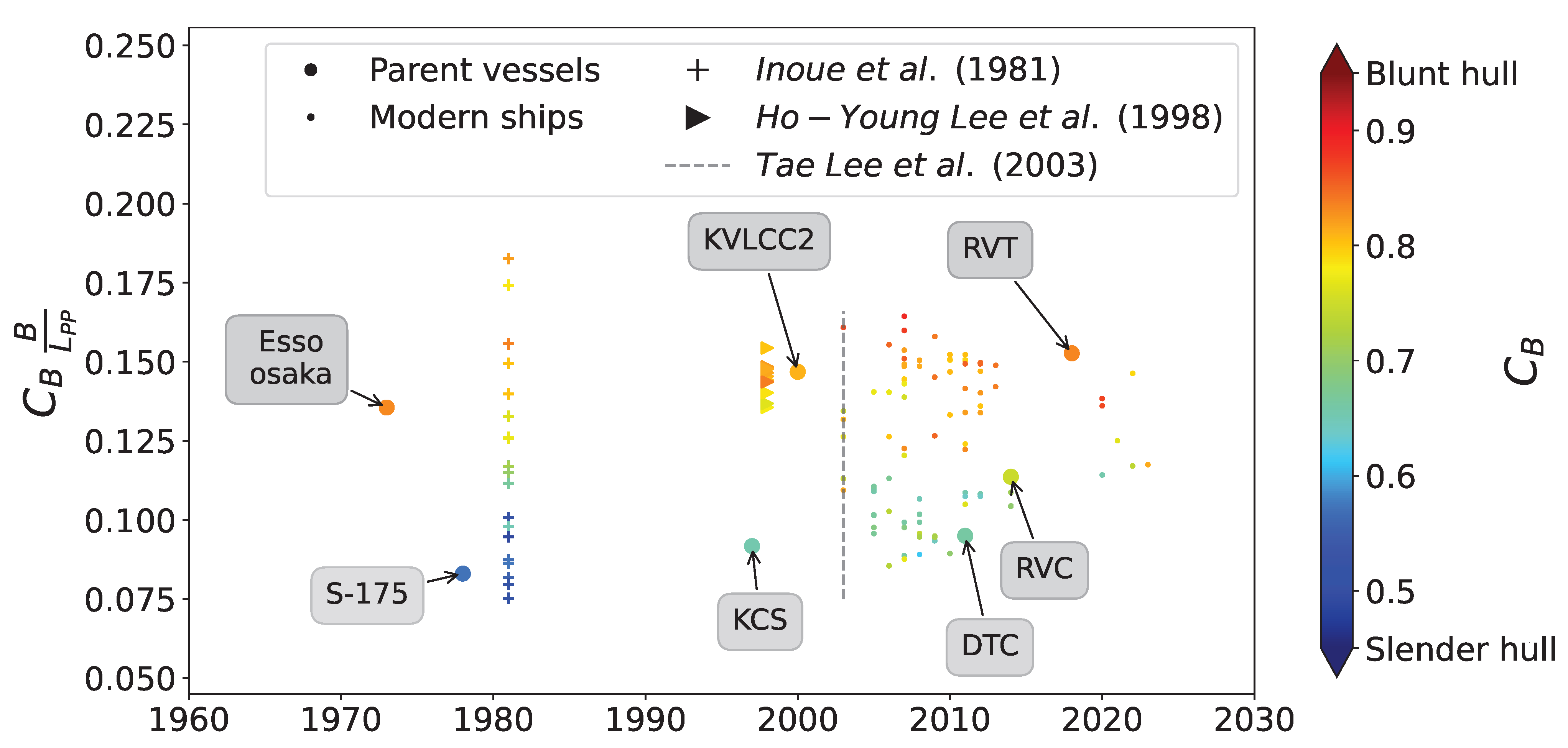
A secondary database comprising 90 contemporary vessels (cargo ships, tankers, and bulk carriers) launched from 2013 onward was compiled using principal dimensions sourced from industry publications like Significant Ships. This resource was used to identify geometric trends by comparing the scatter plot of the non-dimensional parameters between the modern fleet and the databases employed for regression methods. Figure 2 brings an analysis of the $C_{B}B/L$ parameter, a common predictor among the empirical methods. It is easy to distinguish between slender ($C_B<0.75$) and blunt ($C_B>0.75$) hull groups, confirming that the reference vessels adequately represented the modern fleet. While the Lee’s database matched typical modern tankers, a comparison with the database from Inoue et al. [19] shows an increase in the block coefficient in modern vessels; as a consequence, a lack of representation of slender hull forms is expected, consistent with the finding previously discussed.

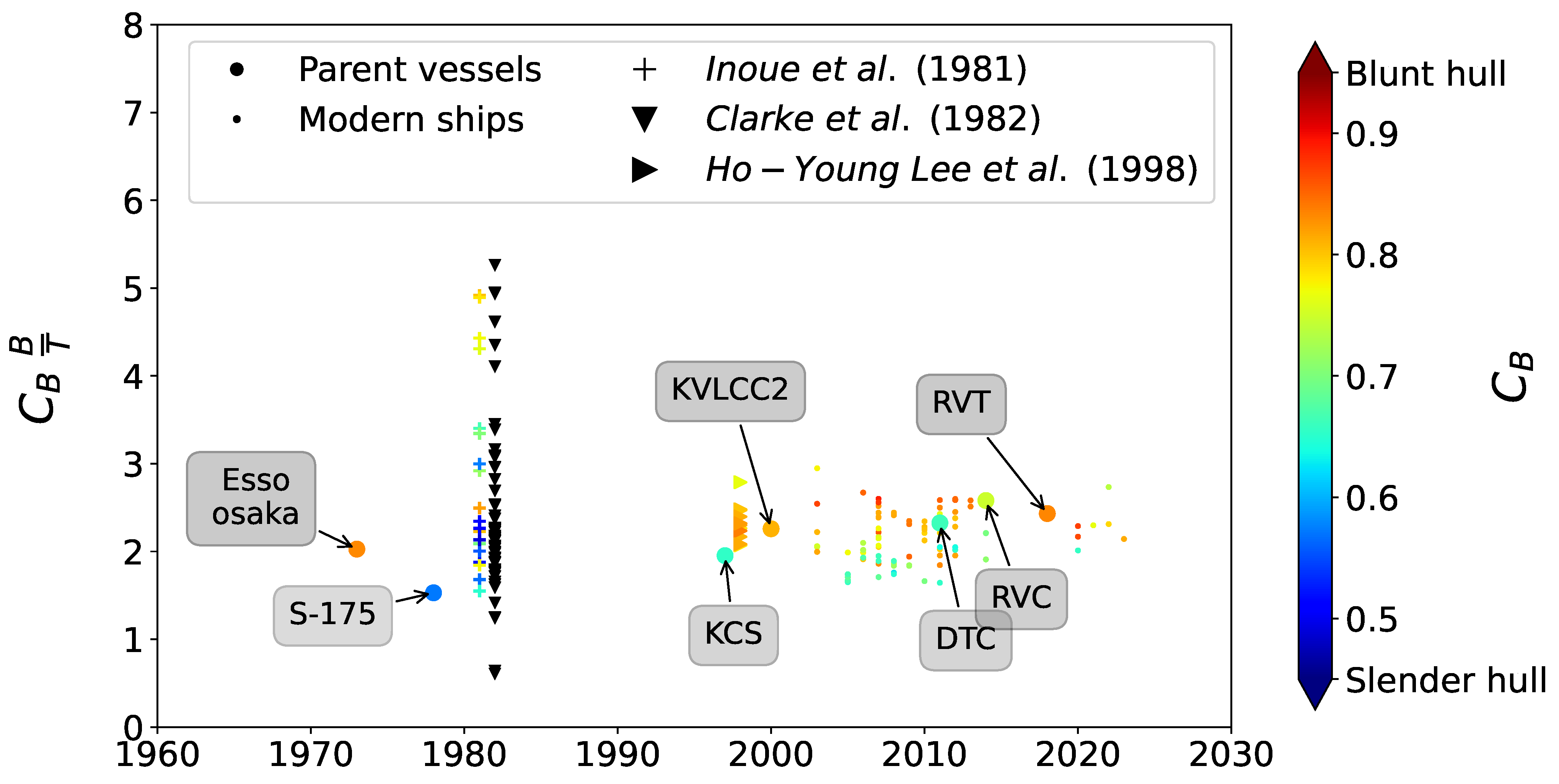
As shown in Figure 3, the databases underlying the empirical formulations exhibited a significantly broader, more scattered distribution of geometric coefficients. At the same time, a narrower and more clustered range of $C_{B}B/T$ values was found for modern hulls. This divergence is highly relevant because, while many classical regression models showed reasonable agreement with modern data when using the coefficient $C_{B}B/L$, the pronounced decrease in the $C_{B}B/T$ ratio is a distinguishing feature of modern designs. This inability of regressions to accurately encompass the shrinking range of $C_{B}B/T$ over time directly accounts for the poor performance observed in the KVLCC2 and KCS benchmark cases. Consequently, incorporating these specific geometric trends is recommended when developing empirical models to predict the linear sway derivative. Neglecting these trends may lead to inaccurate estimates of sway force and, consequently, unreliable predictions of maneuverability.

As noted by [24], using empirical formulas outside the range of their regression databases can yield unreliable predictions of maneuverability. Consequently, further research is necessary to understand how the new design affects maneuvering characteristics, and predictions should be adjusted accordingly.

2.4. Advancements in CFD for Prediction of the Maneuvering Coefficients

Pioneering work by [39] demonstrated the capability of the Finite Volume Method (FVM) to predict hydrodynamic forces in oblique flows, even for complex hull forms, reproducing standard captive model tests such as oblique towing, circular motion, and planar motion mechanism tests. Initial numerical predictions, however, showed a $22\%$ underprediction compared to experimental data. Subsequent extensive verification and validation studies by researchers such as [24,40] confirmed the promising role of viscous flow computations in predicting maneuvering characteristics based on numerically derived hydrodynamic coefficients.

A key metric for evaluating numerical progress is the reduction in prediction error for the lateral force derived from Virtual static drift tests (VSDT).

Table 3. Comparison of the lateral force prediction error obtained through VSDT.

Author	Drift Angle ($\mathit{\beta }$)	Free Surface	Mesh Size [${10}^6$]	${\mathit{Error}}_{\mathit{abs}}$
Ohmori [39]	$9^{\circ }$	-	0.095	$22\%$
Toxopeus [24]	${12}^{\circ }$	-	3.356	$9.2\%$
Fureby et al. [40]	${12}^{\circ }$	-	12.7	$1.7\%$

summarizes key comparisons between numerical studies employing captive model tests. The data reveal a significant improvement in lateral force ($Y^{\prime }$) prediction accuracy over time, which correlates strongly with a substantial increase in computational mesh density. The absolute error dropped from $22\%$ in the late 1990s to $1.7\%$ by the mid-2010s, reflecting major developments in numerical methods and computational power.

Advancements in CFD for hydrodynamic applications have been well benchmarked in blind workshops to validate numerical methods. While historical conferences, such as the Gothenburg Workshop in 2000 or the Lloyd’s Register workshop, focused primarily on ship resistance and scale effects, Workshop on Verification and Validation of Ship Manoeuvring Simulation Methods (SIMMAN) aims to assess up-to-date methods for ship maneuvering prediction. This dedicated workshop serves as a critical metric for evaluating viscous-flow calculations used for static and dynamic maneuvers. Several organizations were invited to submit blind responses to well-specified test cases. The first edition was held in 2008, and participants sent computations performed on meshes of up to 7M cells for the virtual captive model tests. In SIMMAN’20 [38], the largest grid was up to 30M. Over the twelve-year interval, numerical methods for maneuvering proliferated, increasing the number of submissions and resulting in fair prediction accuracy; for example, SIMMAN’20 reported an average error of $6.5\%$ for oblique force predictions. This growing reliance on computational methods enhances the efficacy of maneuvering prediction, and the data collected on numerical settings (such as the widespread use of the double-body model for the air–water interface and the k-$\omega$ SST turbulence model) provide essential guidance for future research. Ref. [41] numerically examines the effects of bulbous bows on the hydrodynamic forces acting on a tanker-shaped hull by conducting virtual static drift tests and compares the maneuverability of three bow-variant ships. Among the hulls tested, the one with a protruding bow experiences the lowest linear sway velocity derivative, whereas those with a shrink bow experience larger lateral forces. Most previously introduced empirical formulations were derived from experimental results based on a database of hulls with shrink bulbous bows, and there is a need for a deeper understanding of how this apparatus will affect maneuvering performance. Ref. [42] employed virtual captive model tests to propose new maneuvering coefficients of an Abkowitz-type maneuvering model, incorporating water depth-dependent correction on each component. The authors conducted RANS simulations at five different depth-to-draft ratios to build the new approach. Their model was validated against reference cases, demonstrating that CFD can be applied to complex problems such as shallow-water flows.

3. Numerical Modeling of Oblique Flow Hydrodynamics

3.1. Mathematical Model for Ship Maneuvering Prediction

Ship maneuvering dynamics are commonly analyzed considering three degrees of freedom (DoF): surge, sway, and yaw [43]. This formulation is sufficient for low-speed applications typical of maneuvering simulations, where roll, pitch, and heave are often deemed less significant. A convenient coordinate system is defined to compute the hydrodynamic forces and moments acting on the ship. This system is called a body-fixed frame ($o-xyz$) and has its origin coincident with the midship of the hull on the waterplane. As shown in Figure 4, the x-axis points to the bow and the y-axis to the port. Additionally, an earth-fixed coordinate ($O-XYZ$) system is adopted to describe the ship’s motion, where $\psi$ denotes the heading angle (rate of turn $\dot{\psi }=r$).

The equation of motion on three degrees of freedom for surface ship maneuvering prediction is

$$\begin{array}{c}(M+M_{11})\dot{u}-(M+M_{22})vr-(M{x}_G+M_{26})r^2=F_{X,tot}\\ (M+M_{22})\dot{v}+(M{x}_G+M_{26})\dot{r}+(M+M_{11})ur=F_{Y,tot}\\ (I_Z+M_{66})\dot{r}+(M{x}_G+M_{26})(\dot{v}+ur)+(M_{22}-M_{11})uv=N_{Z,tot},\end{array}$$

(3)

in which the left side is the total forces and moment in the x, y, and z-direction, respectively. The fluid inertia tensor is defined by $M_{ij}$, with $i,j=[1,6]$, i.e., $M_{11}$ and $M_{22}$ represent the ship-added masses in the surge and sway directions, respectively. $M_{66}$ is the ship-added moment of inertia and $M_{26}$ is coupled sway-yaw added inertia. The position of the center of gravity in the horizontal plane is assumed to be along the ship’s centerline, i.e., $y_G=0$. $F_X$, $F_Y$, and $N_Z$ correspond to the longitudinal force, lateral force, and yaw moment, respectively. The subscript tot indicates the total force, which is defined as the sum of both potential and external loads. In the modular approach (MMG), this total force is decomposed into distinct components depending on the phenomenon one wants to model. The methodology operates under key assumptions, including treating the ship as a rigid body under quasi-steady hydrodynamic conditions while disregarding wave-making effects due to low-speed operations [44].

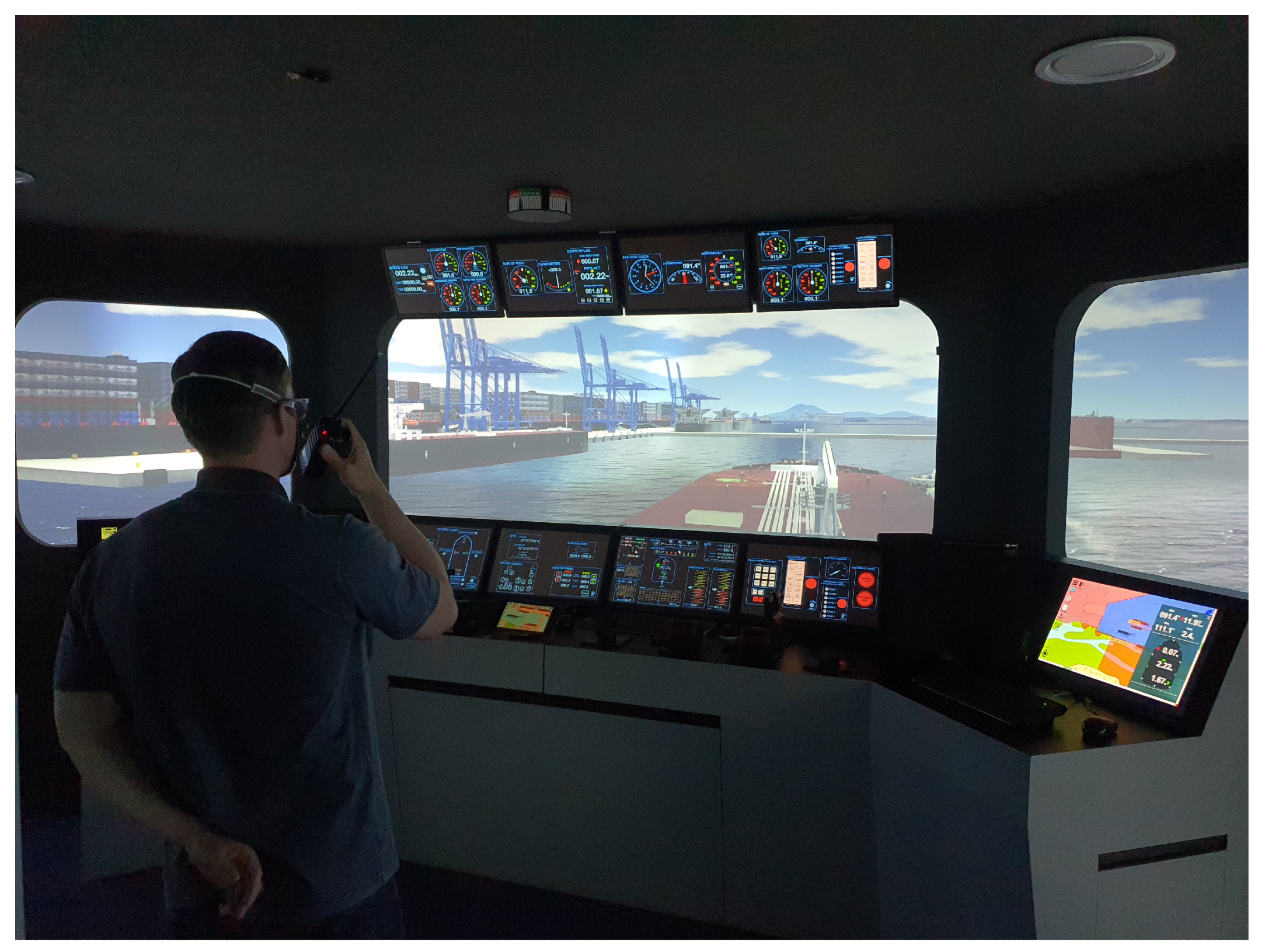
The simulation capabilities described herein are based on the in-house mathematical model, hereafter called Numerical Offshore Tank Mathematical Model (MM-TPN). This model is rooted in a quasi-explicit heuristic approach for estimating ship maneuvering forces, initially proposed by [45] and subsequently refined by [46]. The comprehensive numerical implementation is detailed in [47]. Besides, TPNMM follows the ITTC procedures to calibrate and validate maneuvering models. The full-mission simulator used in this study is entirely developed in-house at TPN-USP, relying on a proprietary simulation platform that integrates a Unity-3D visualization system and a C++ computational engine running the MM-TPN maneuvering model, environmental-force modules, and the control-and-command interface. TPN Ship Maneuvering Simulation Center Also called Maritime and Waterways Simulator of the Numerical Offshore Tank (SMH). is the largest of its kind in Brazil. The center comprises six simulators, three classified into full-mission, which means an immersive system with more than ${270}^{\circ }$ of projection and three tug stations. Furthermore, the simulators can be adapted to represent different kinds of vessels and operate individually or combined. Figure 5 shows the main full-mission simulator.

The MM-TPN is a modular model (MMG) that analyzes the total force ($F_{tot}$) acting on the vessel by decomposing it into component, expressed as

$$F_{tot}=F_{hydro}+F_{wind}+F_{wave}+F_{rudder}+F_{prop}+F_{ship-ship}+F_{bank}+F_{tug}+F_{mooring}.$$

(4)

The non-potential hydrodynamic loads ($F_{hydro}$), a leading component, are determined via sectional integration along the vessel’s length ($L_{PP}$). The longitudinal force ($F_{X,hydro}$), lateral force ($F_{Y,hydro}$), and yaw moment ($N_{Z,hydro}$) are calculated using

$$\begin{array}{c}{F}_{X,hydro}={\displaystyle \frac{1}{2}}\rho T{\int }_{\frac{-L_{PP}}{2}}^{\frac{L_{PP}}{2}}{C}_{1C}\left({\psi }_{crx}\right){\overrightarrow{V}}_{crx}^{2}dx,\hfill \end{array}$$

(5)

$$\begin{array}{c}{F}_{Y,hydro}={\displaystyle \frac{1}{2}}\rho T{\int }_{\frac{-L_{PP}}{2}}^{\frac{L_{PP}}{2}}{C}_{2C}\left({\psi }_{crx}\right){\overrightarrow{V}}_{crx}^{2}dx,\hfill \end{array}$$

(6)

$$\begin{array}{c}{N}_{Z,hydro}={\displaystyle \frac{1}{2}}\rho T{\int }_{\frac{-L_{PP}}{2}}^{\frac{L_{PP}}{2}}(C_{2C}\left({\psi }_{crx}\right){\overrightarrow{V}}_{crx}^2-C_{2C}\left(\psi \right){\overrightarrow{V}}_{cr}^2)xdx+{\displaystyle \frac{1}{2}}\rho T{L}_{PP}^2{C}_{6C}\left(\psi \right){\overrightarrow{V}}_{cr}^2.\hfill \end{array}$$

(7)

Here, ${\overrightarrow{V}}_{cr}$ and ${\overrightarrow{V}}_{crx}$ represent the midship and sectional relative velocities, respectively. The angle ${\psi }_{crx}$ defines the relative incidence of the water at each section of the vessel. The model is based on the integration of the forces acting on each section of the vessel. The formulation presented herein was modified to accommodate the numerically obtained coefficients rather than empirically derived ones. Thus, following the approach described by Leite et al. [45], the lateral force coefficient can be calculated using the formulation given by

$$C_{2C}=(C_Y-{\displaystyle \frac{\pi T}{2L}})sin\psi \left|sin\psi \right|+{\displaystyle \frac{\pi T}{2L}}{sin}^3\psi -Y_v^{\prime }sin\psi \left|cos\psi \right|·$$

(8)

Let $C_{2C}$ be the lateral force coefficient, and it will require the calculation of the cross-flow drag coefficient ($C_Y$), and linear sway velocity derivative ($Y_V^{\prime }$). The lateral force coefficient can be determined using the forces obtained numerically for the selected drift angles: $\beta$=$0,2,4,6,8,10$, and ${12}^{\circ }$.

3.2. Computational Method

In the context of maneuverability, accurate prediction requires determining the lateral force (Y) and yaw moment (N) across a range of drift angles ($\beta$). The resulting linear hydrodynamic coefficients are derived from the slope between the non-dimensional force or moment and the corresponding $sin\beta$. Hydrodynamic forces in oblique motion can be obtained through experimental model tests or numerical computation. The virtual domain approach, adopted here, determines relative fluid-hull velocity by setting an inlet speed and adjusting the hull’s orientation to achieve the required drift angle, a technique favored over prescribing incidence angle directly to the velocity to mitigate potential mesh alignment issues.

Within the scope of this research, it is necessary to determine the phenomena that require modeling and which simplifications can be made without losing accuracy. Since the results obtained herein will be used to derive the linear hydrodynamic derivatives, and considering that several conditions of drift must be addressed, a numerical method that computes these forces as quickly as possible is expected. However, some assumptions made to derive the MMG yield a considerable simplification in the numerical setup. Within the background discussed in the previous sections, an overview of the assumptions is explored next.

3.2.1. Physical and Numerical Modeling

Accurately describing the flow of water around a maneuvering ship hull remains an intricate challenge in ship hydrodynamics [5]. To balance accuracy with computational efficiency necessary for deriving linear hydrodynamic derivatives across multiple drift conditions, specific modeling assumptions derived from the structure of the mathematical model (MMG) are implemented:

1.

Bare Hull Analysis: Consistent with the mathematical model derivation, calculations focus exclusively on the bare hull. The effects of the propeller and rudder are excluded and accounted for separately by the TPNMM.

2.

Free Surface Neglect (Double Body): Given the low-speed maneuvering regime ($F_r<0.2$) relevant to the MMG derivation, free surface disturbances are disregarded. The air–water interface is treated as a plane of symmetry (double body assumption). This simplification drastically reduces computational cost (potentially by 1000% [48]) and is acceptable for drift angles up to ${15}^{\circ }$ [49].

3.

Attached Flow and Linear Regime: The focus on deriving linear hydrodynamic derivatives necessitates computing forces within the linear regime, typically confined to small drift angles ($\beta \le {12}^{\circ }$). The flow is consequently assumed to be primarily attached, reflecting large-scale flow over the hull [5].

4.

Model Scale Computation: Calculations are conducted at the model scale, relying on the observed weak dependence of $Y^{\prime }$ and $N^{\prime }$ on Re within the linear regime [5].

5.

Steady-State Flow: To accurately predict the hydrodynamic forces in oblique flow, a steady-state computation is proposed for drift angles up to ${12}^{\circ }$. This assumption is valid since pressure and velocity are not expected to vary temporally once the flow is fully developed in the VSDT scenario.

Based on these considerations, the numerical model addresses an incompressible, steady-state, turbulent, single-phase flow around the bare hull. The Reynolds-Averaged Navier–Stokes (RANS) equations are employed, utilizing the two-equation Shear Stress Transport (SST) $k-\omega$ closure model, based on the updated version proposed by [50]. Calm, unrestricted, and deep water conditions are modeled.

3.2.2. Computational Domain and Boundary Conditions

All grids were generated using native OF utilities. Initially, a base hexahedral volume mesh was constructed using the blockMesh utility, where the domain was partitioned into twenty-four sub-domains primarily to control mesh grading. This base meshing process was initialized in the region near the future location of the geometry (the domain origin) and propagated outwards toward the walls. Following this, the snappyHexMesh tool was employed to integrate the hull geometry into the domain and generate the final hybrid mesh, ensuring the grid adequately captures the physical phenomena in the near-hull region.

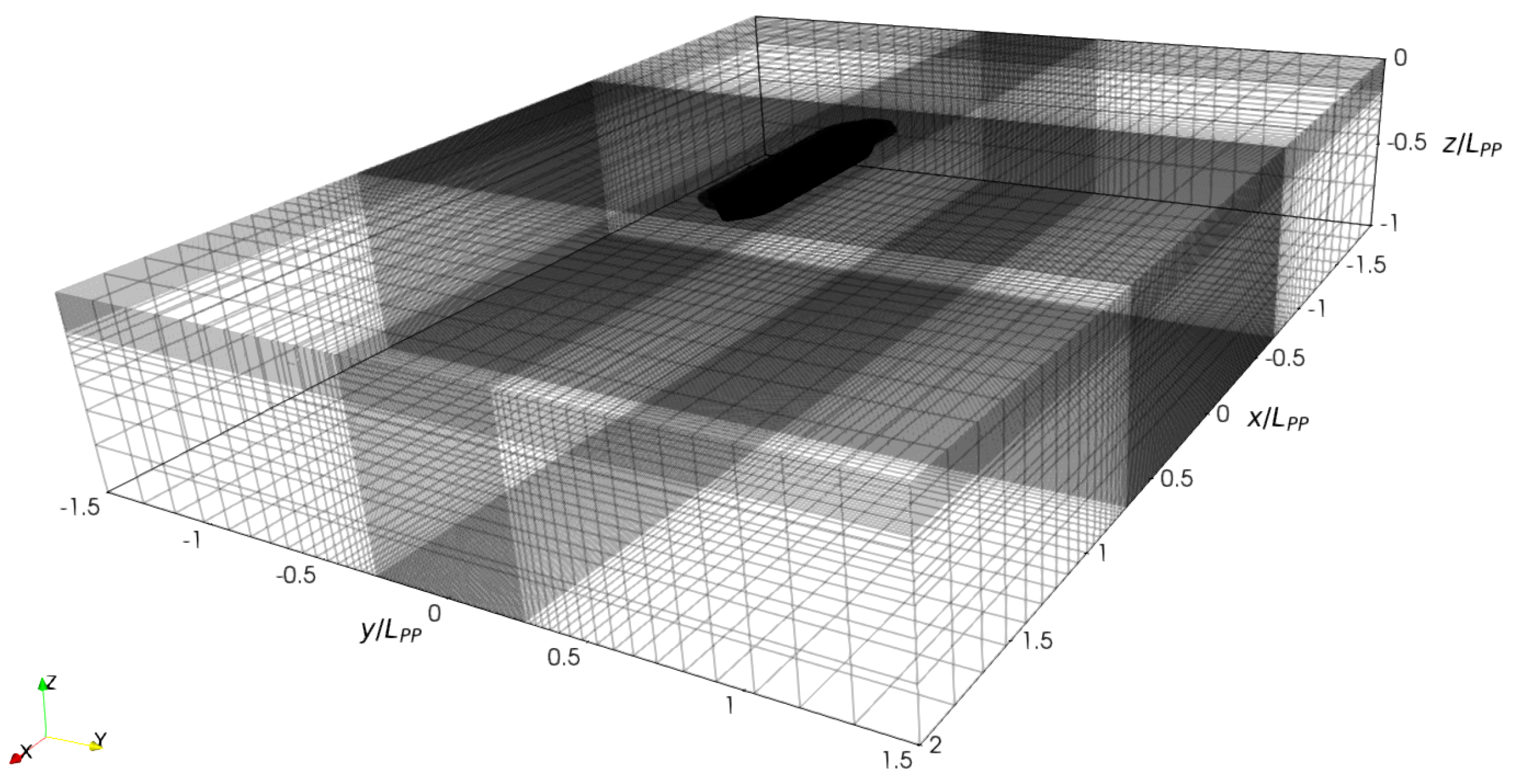
Regarding the domain size, the International Towing Tank Conference (ITTC) recommends a minimum of one length from the bow to the inlet for resistance cases. However, due to the slight drift angles of interest, the domain length was extended to 2L_PP. To minimize the potential for blockage effects associated with oblique flows, the side walls were judiciously positioned $1.5$L_PP from the midship. Figure 6 illustrates a sketch of the virtual towing tank. The fluid domain comprises four distinct regions, among which zone00 was the most heavily refined. Contrasting with standard mesh generation practices where the global largest cell size is the reference, the refinement element here—the near-wall cell height ($y_n$)—is defined within zone00 (i.e., adjacent to the hull). Consequently, the grid independence study was performed exclusively by varying this established reference element.

Figure 7 shows an example of the final mesh. To efficiently generate computational grids for various hull forms and drift angles, an automated procedure was developed. This procedure creates the mesh based on the hull’s main dimensions and the required drift angle. All generated meshes consistently met the quality criteria outlined in the OF manual, specifically adhering to the maximum skewness threshold of four and maintaining the aspect ratio fixed at ten during the background mesh stage.

3.3. Verification and Validation Procedure

Verification confirms the quality of the numerical treatment and implementation, while Validation ensures the mathematical model accurately represents the physical problem within acceptable limits. Following established guidelines [51,52,53]. The validation criterion is satisfied if the comparison error ($E=D-S$, where D is benchmark data and S is the simulated quantity) is less than the validation uncertainty ($U_V$), defined as $U_V=\sqrt{U_D^2+U_{SN}^2}$, where $U_D$ and $U_{SN}$ are the data and numerical uncertainties, respectively.

Numerical uncertainty ($U_{SN}$) was primarily assessed through grid convergence ($U_G$), as iterative uncertainties ($U_I$) were negligible ($U_I\ll U_G$). Grid convergence employed three or more systematically refined meshes ($m\ge 3$) with a constant refinement ratio $r_G=\sqrt{2}$. Key parameters used in this verification process, including the convergence ratio ($R_G$) and Grid Convergence Index ($GCI$), and order of accuracy (p). Monotonic convergence ($0<R_G<1$) allowed the application of generalized Richardson Extrapolation (RE) to estimate the order-of-accuracy (p) and the asymptotic numerical solution ($f_{G0}$), which can be determined by

$$f_{G0}=F_{X,Richardson}={\displaystyle \frac{r_G^p{\varphi }_1-{\varphi }_2}{r_G^p-1}}·$$

(9)

Four standard hull forms (Esso Osaka, KVLCC2, S-175, and KCS) were investigated under static drift conditions (captive tests) using the double-body hypothesis, with wave resistance effects neglected. Steady-state single-phase computations were performed to obtain the hydrodynamic forces and moments under different conditions. Some of these numerical results were validated against benchmark cases, shown in

Table 4. Validation data for the captive tests.

		Type	Model	$\mathit{\lambda }$	${\mathit{F}}_{\mathit{r}}$	Exp. Data
Esso Osaka
Resistance
$\beta =0^{\circ }$	[54]	CPMM	BH	43	0.063	$C_T=$−0.0047
Static drift
$\beta =4^{\circ }$	[54]	CPMM	BH	43	0.063	$Y^{\prime }=$ 0.0295
KVLCC2
Resistance
$\beta =0^{\circ }$	[55]	TT	AH	58	0.142	$C_T=$−0.0041
Static drift
$\beta =4^{\circ }$	[56]	TT	BH	64	0.142	$Y^{\prime }=$ 0.0178
$\beta ={12}^{\circ }$		TT	BH	64	0.142	$Y^{\prime }=$ 0.0717
S-175
Resistance
$\beta =0^{\circ }$	[57]	TT	AH	43	0.15	$C_T=$−0.0029
Static drift
$\beta =4^{\circ }$	[20]	-	AH	58	0.20	$Y^{\prime }=$ 0.0150
$\beta =8^{\circ }$		-	AH	58	0.20	$Y^{\prime }=$ 0.0370
KCS
Resistance
$\beta =0^{\circ }$	[58]		AH	65	0.26	$C_T=$−0.0037
$\beta ={12}^{\circ }$	[38]	CMT	RH	105	0.21	$Y^{\prime }=$ 0.0685

Notes: In this, the acronyms CPMM, CMT, and TT stand for captive planar motion mechanism, circular motion test, and towing tank tests, respectively. The model can be described as appended (AH), a model with a rudder and w/o propeller (RH), or a bare hull (BH).

.

For the Esso Osaka tanker, the longitudinal force prediction at $\beta =0^{\circ }$ exhibited oscillatory convergence but was successfully validated with a 5.28% numerical uncertainty. For the static drift case ($\beta =4^{\circ }$), all integral quantities ($F_X,F_Y,M_Z$) achieved monotonic convergence and were validated at a low uncertainty level. The containership S-175, which lacks a bulbous bow and transom stern, was selected for validation due to the availability of oblique flow experimental data conducted at a low Froude number, which aligns with the assumptions of the numerical model. However, the validation process faced significant challenges: experimental data from [20,57] only considered the appended hull, introducing unavoidable deviations from the bare hull CFD results, and the data lacked clear information regarding methodology and experimental uncertainty, leading to the adoption of a conservative $5\%$ standard uncertainty. While the longitudinal resistance validation met the scope’s objectives, the lateral force and yaw moment validation was limited to verification due to the influence of the propeller and rudder on the numerical results.

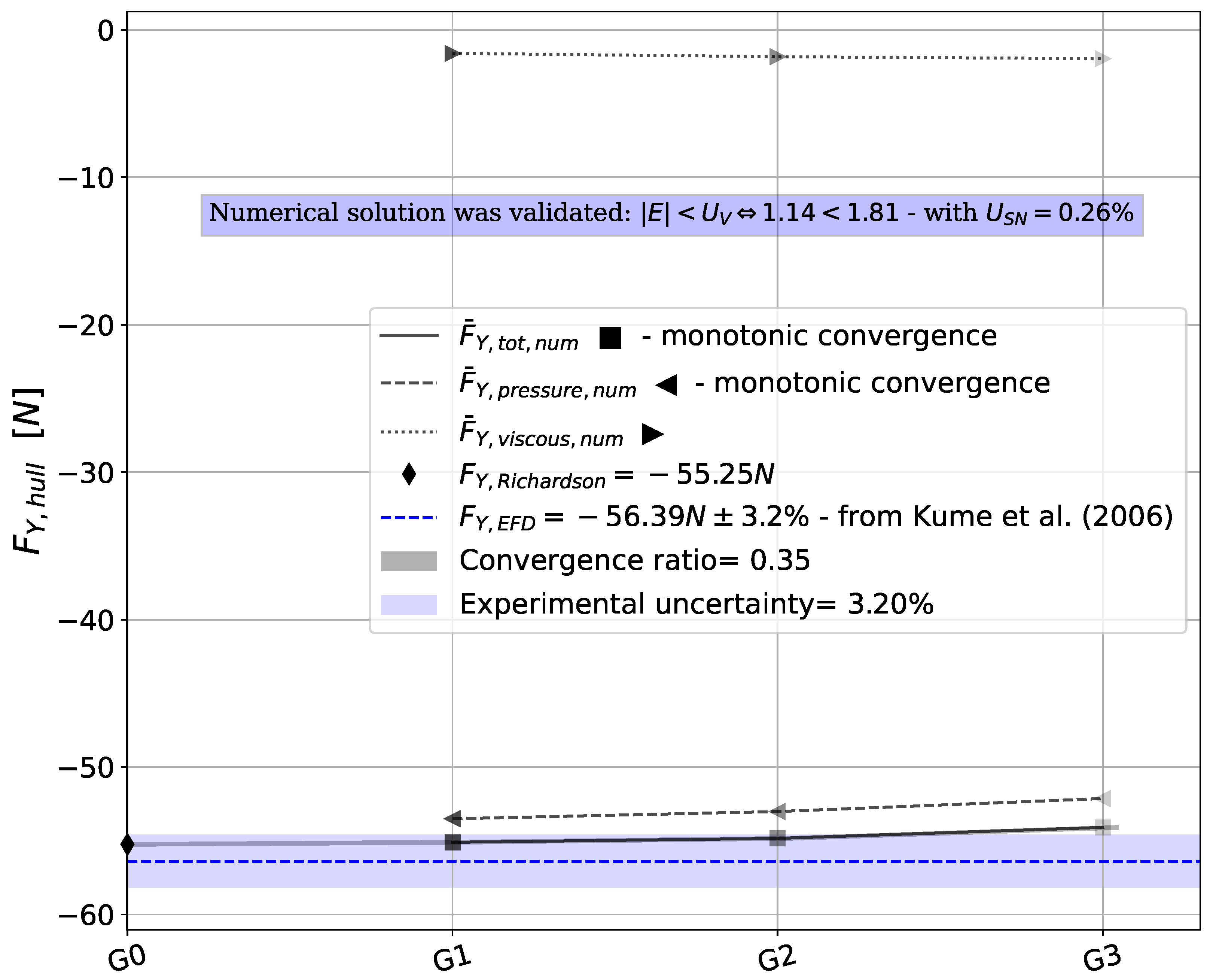
The modern KVLCC2 tanker was extensively studied, including a robust five-mesh convergence analysis for resistance ($\beta =0^{\circ },F_r=0.142$), achieving an asymptotic range and a very small numerical uncertainty ($U_{SN}=0.26\%$). Additionally, the computed value was close to the experimental data [55], with a discrepancy of less than $1\%$. Crucially, the numerical model demonstrated its ability to predict lateral force ($F_Y$) accurately and yaw moment ($M_Z$) in high oblique flow. Validation of $F_Y$ at $\beta ={12}^{\circ }$ showed good agreement with experimental results, confirming model suitability up to this drift angle, as illustrated in Figure 8.

Verification results for the KCS containership confirmed that the numerical uncertainty for the total forces was well within established limits ($U_{SN}<5\%$), even for the lateral force ($F_{Y,tot}$) at $\beta ={12}^{\circ }$, which showed $U_{SN}<3\%$ via Richardson Extrapolation. Computational time analysis indicated that the model efficiently calculates these forces, with the fine mesh ($G1$) requiring approximately 15 h on 20 cores. Hardware description is thoroughly explored in [36].

In conclusion, the established CFD methodology provides reliable predictions of hydrodynamic forces and moments in static drift conditions, having been rigorously verified and validated against benchmark data up to a ${12}^{\circ }$ drift angle, achieving numerical uncertainties consistently below the target threshold. This established methodology is suitable for the subsequent determination of hydrodynamic maneuvering coefficients.

4. Prediction of the Maneuvering Coefficients

4.1. Analysis of Hydrodynamic Coefficients at Low Drift Angles ($\beta \le {12}^{\circ }$)

The accurate prediction of ship maneuvering requires isolating the linear components of hydrodynamic forces and moments, particularly at low drift angles. Following the classical approach established by [5], the non-dimensional lateral force ($Y^{\prime }$) is often decomposed into linear and nonlinear contributions, resulting in

$$Y^{\prime }=(a_{o}cos\beta +C_Y|sin\beta |)sin\beta ,$$

(10)

where $a_o$ is the lift-curve slope taken from small drift angles, and $C_Y$ is the cross-flow drag coefficient (Ref. [36] suggested a value near 0.7 for tankers).

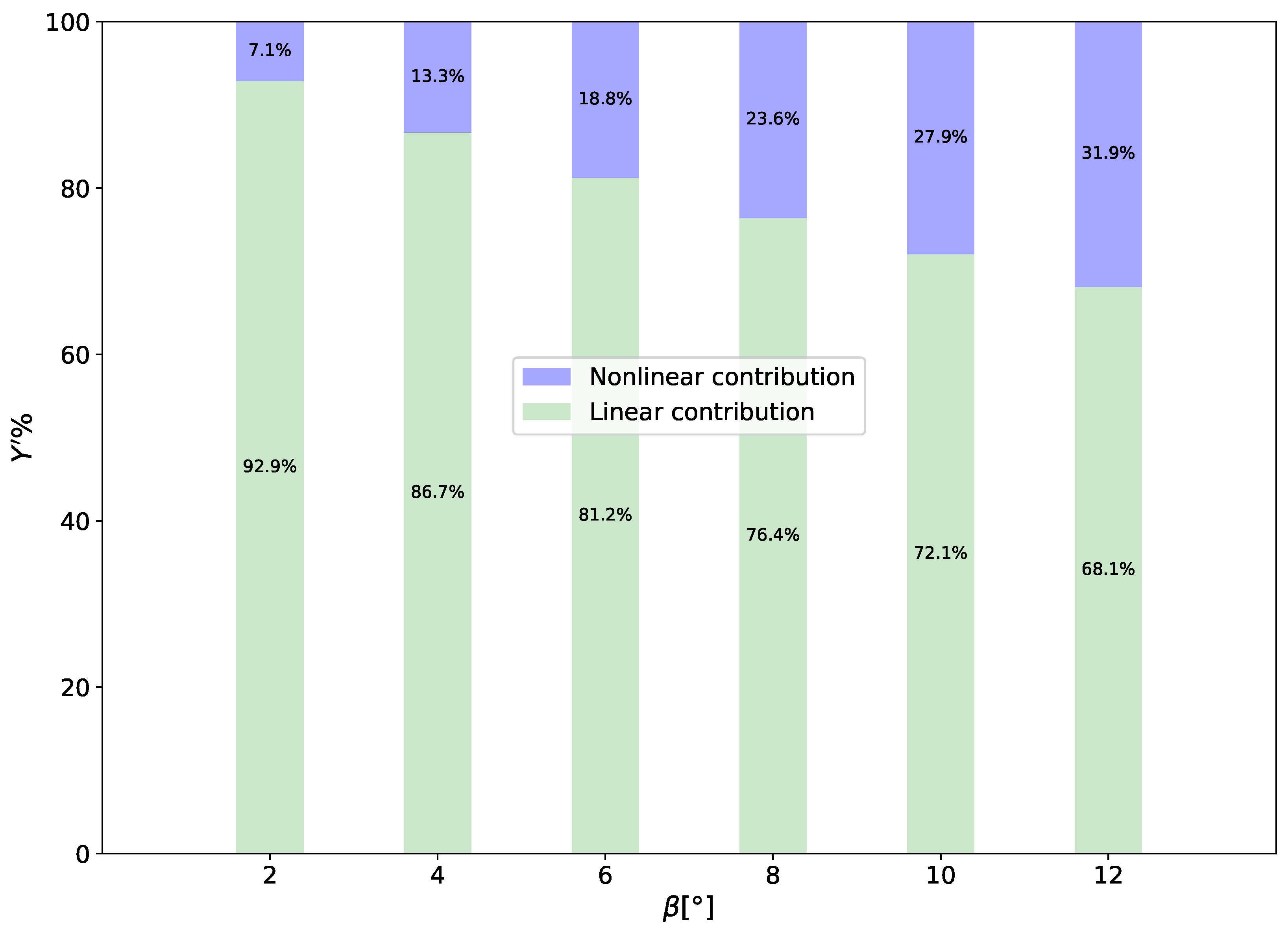
An examination of the force decomposition confirms that the linear contribution ($a_o$) is dominant near $\beta =0^{\circ }$. Although the nonlinear cross-flow drag contribution is almost negligible for small angles, it increases rapidly after $\beta \approx {10}^{\circ }$. This observation suggests that the range of angles used to derive the linear derivative ($Y_V^{\prime }$) must be sufficiently large to capture the linear trend accurately, yet constrained enough to minimize the influence of growing nonlinear effects (as illustrated in Figure 9). The central premise for maneuvering prediction, particularly within models like the TPNMM, is that the required linear derivative is derived from the initial linear slope, with the nonlinear contribution subsequently modeled separately, even at small angles.

4.2. Derivation of Linear Hydrodynamic Derivatives

The linear derivatives are extracted by fitting a slope between the non-dimensional force or moment and the $sin\beta$ predictor, interpreted as a Regression Through the Origin (RTO). Figure 10 schematically shows how the linear derivative will be determined. The diagram indicates that the regression is through the origin (RTO), and the y-axis represents the linear lateral force computed by means of the virtual static drift test.

The sway velocity derivative ($Y_V^{\prime }$) is formally defined by

$$\begin{array}{c}\hfill Y^{\prime }=Y_v^{\prime }sin\beta ,\end{array}$$

(11)

where $Y^{\prime }$ is the lateral force obtained numerically (also called $F_{Y,tot}$). The regression coefficient derived from these equations is adopted as the linear derivative (as schematically represented in Figure 10). This hypothetical plot allows some reflections on how the data behaves as the values of the predictor ($sin\beta$) change. First, an outlier in this situation is unexpected, and if it appears, it may indicate an issue in the numerical prediction. In ordinary linear regression analysis, the focus lies on finding a formulation to predict future dependent variables based on a coefficient assumed constant within the model’s range of applicability. Conversely, the specific goal herein is to uniquely determine this regression coefficient and adopt its value directly as the linear derivative. A last reflection can be built on the main idea of these two worlds: on the one hand, one wants to find the linear derivative using the theory of linear regression; on the other hand, in statistics, it is expected that the slope behaves near a straight line. Notwithstanding, the linearity assumption should be addressed in both subjects.

From a statistical perspective, linear regression is valid if certain criteria are met. For this, a set of parameters must be assessed. Additionally, visual analysis of the predicted values can be beneficial for this task. One approach is to check the residual plot; if it is well-behaved, the problem is nonlinear. From a maneuvering perspective, a more abstract analysis is expected; flow-field analysis may help with this. Nonetheless, this is a Chicken-and-Egg problem, since the implications of the numerical model were based on the assumption of attached flow due to the expected linearity of the problem at small drift angles, and by employing such a numerical model, one can fail to capture all the physics.

Statistical analysis ensures the validity of the linear assumption. Key metrics for evaluating the regression model’s performance include the R-squared ($R^2$), which ideally approaches unity, indicating the model accounts for the majority of the dependent variable’s variation, and low standard error ($SE$) and p-values.

4.3. The Linear Drift Angle Limit

4.3.1. Linear Derivatives of Blunt Bodies

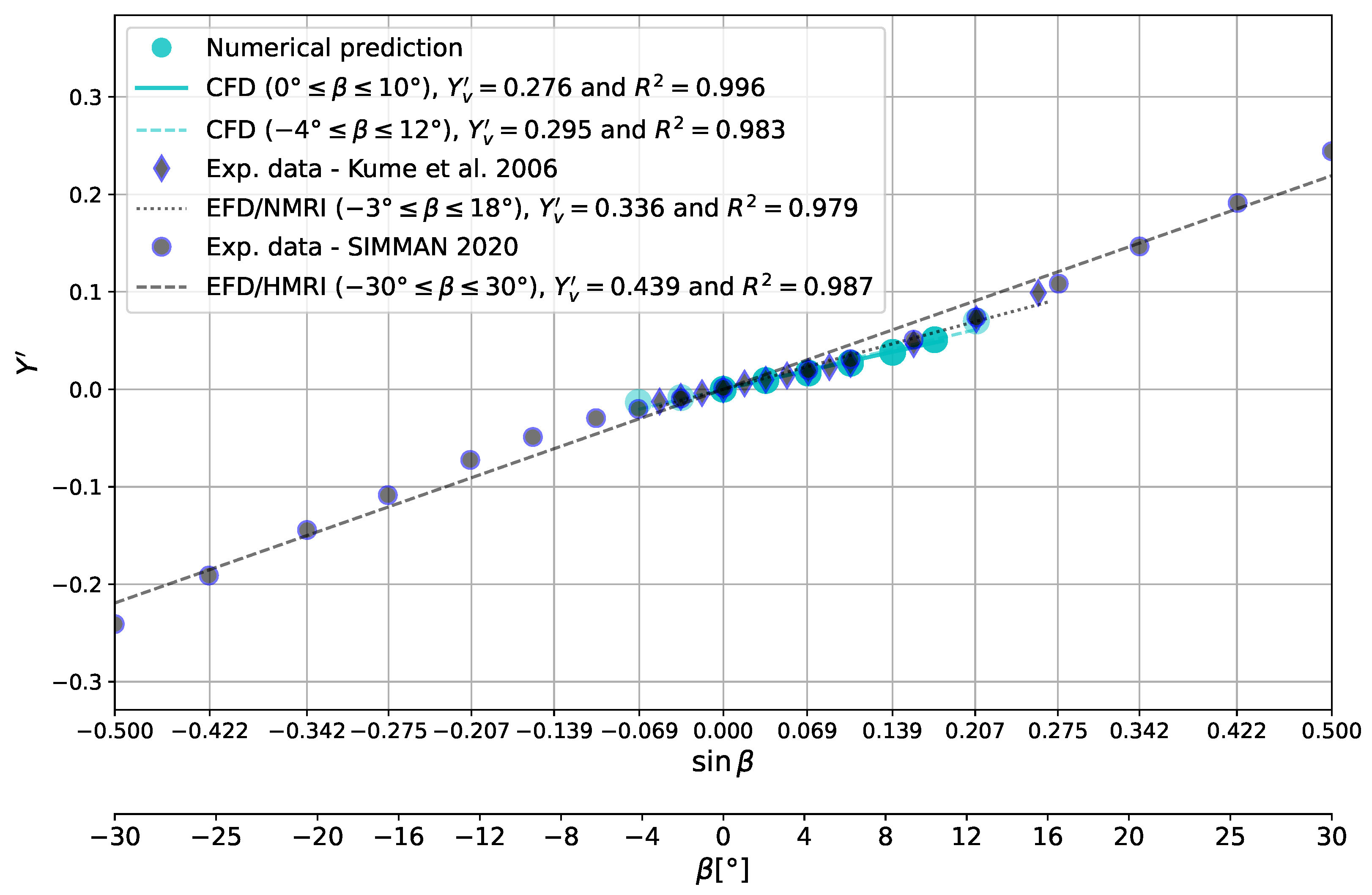
For the KVLCC2 tanker, comparisons were drawn between CFD results and two sets of experimental data provided by SIMMAN’20 workshop to validate mathematical models to predict maneuverings. Planar Motion Mechanism (PMM) experiments were performed on the appended ship at Froude number 0.142, and the model was scaled to 1:46. Conversely, the NMRI conducted another set of experiments, at the same $Fr$, on the bare hull scaled at $\lambda =64$. Unlike the facility used previously, an oblique towing tank was employed. As a consequence, issues related to frequency dependence were diminished in this campaign. In Figure 11, all the data provided by the workshop and those reported by [56] were plotted within the numerical prediction.

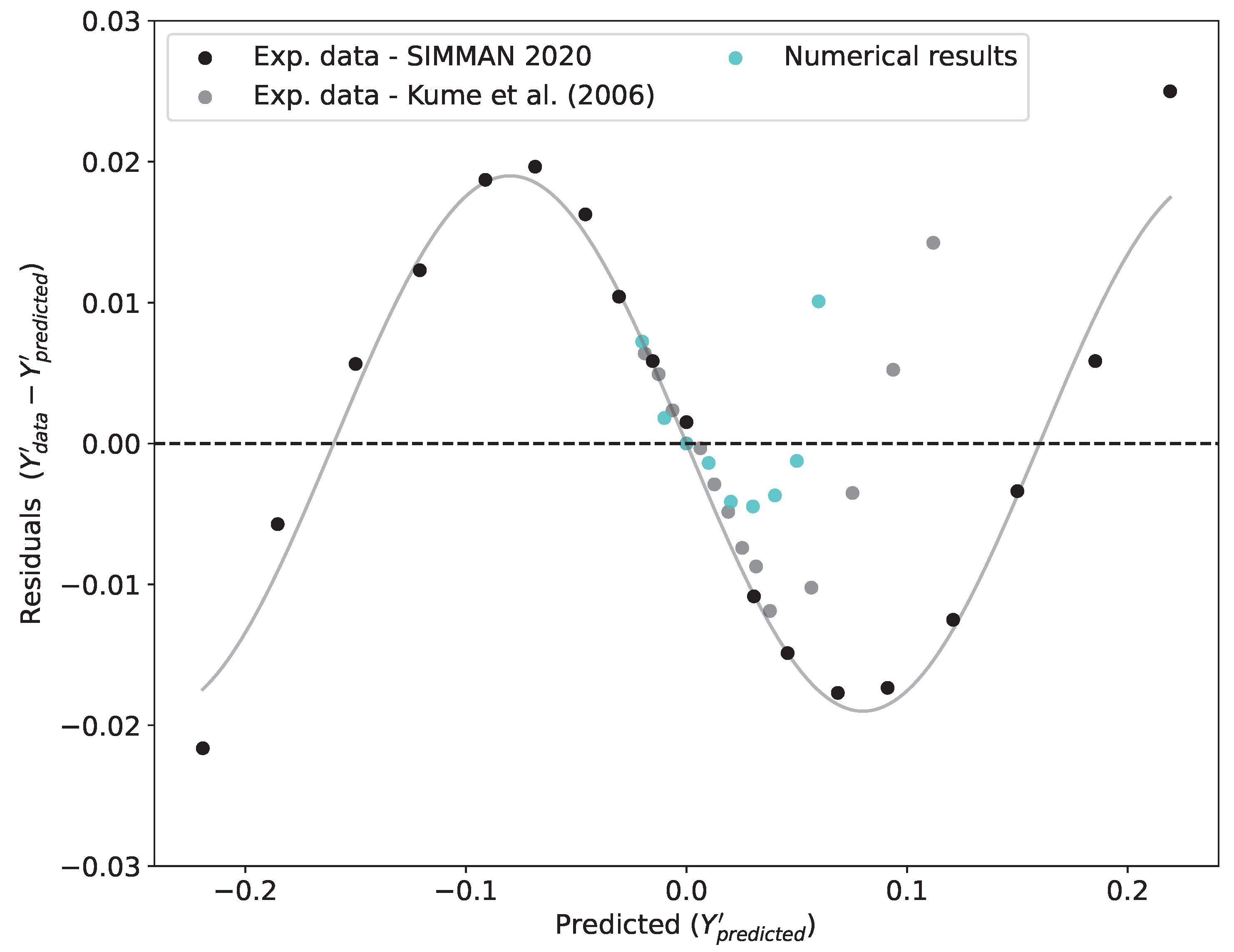
The EFD-HMRI data, due to appended configuration and frequency-dependent testing, exhibited significant nonlinearities beyond $\beta ={10}^{\circ }$. Residual analysis confirmed this, showing a distinct sine pattern (Figure 12), which violated the linear assumption, even when a linear fit yielded a high $R^2$. Several factors contribute to potential nonlinearities and discrepancies in hydrodynamic derivative measurements. Despite the nonlinear trend, the inclusion of the propeller and rudder significantly impacts results; notably, studies show differences exceeding $25\%$ in lateral force measurements between bare and fully appendaged hulls [44].

Furthermore, the reliance of classical maneuverability models on the quasi-steady state theory necessitates derivatives obtained at zero-frequency tests (e.g., oblique towing). However, the frequency dependence intrinsic to PMM results compromises the linear assumption, a difficulty highlighted even in MMG guidelines [44]. While low-frequency PMM tests may yield results equivalent to static methods, reporting on this crucial subject is often scarce, demanding caution in derivative comparisons. Discrepancies between static and dynamic tests confirm this issue, with PMM results yielding lateral velocity derivatives up to $20\%$ higher than those obtained from static tests in some literature [59].

The experimental data from the NMRI and the numerical data obtained in this work were analyzed using linear regression. This model was considered adequate by analyzing both the statistical metrics and the residual plot. Two different regression models were utilized for each data set, and the statistical results are presented in

Table 5. Summary of the linear regression statistics of KRISO Very Large Crude Carrier 2 (KVLCC2).

				${\mathit{Y}}_{\mathit{V}}^{\prime }$
Case	RM	${\mathit{\beta }}_{\mathit{min}}$	${\mathit{\beta }}_{\mathit{max}}$	${\mathit{Y}}_{\mathit{V}}^{\prime }$	${\mathit{R}}^{\mathbf{2}}$	$\mathit{SE}$	$\mathit{p}$
01—CFD	L	0	10	0.276	0.996	0.003	0.000
02—CFD	L	0	12	0.300	0.988	0.013	0.000
03—EFD/NMRI	L	0	10	0.276	0.994	0.008	0.000
04—EFD/NMRI	L	0	12	0.307	0.985	0.013	0.000
05—EFD/HMRI	L	0	12	0.3345	0.995	0.012	0.002
06—EFD/HMRI	NL	−2	16	0.2716	0.998	0.002	NP

Note: The column name $RM$ describes the order of the regression model; in this, L stands for linear, and $NL$ denotes nonlinear fitting. $AM$ is the method employed to acquire the data. Experimental data were taken from Kume et al. [56] and Quadvlieg and Stern [38]. The nonlinear results (derivatives and statistics) were taken directly from the SIMMAN report, and the $p$-value was not provided (NP). Meanwhile, the linear regression was obtained using the experimental data points.

.

Restricting the range of analysis to smaller angles was crucial. When limited to $\beta \in [0^{\circ },{10}^{\circ }]$, the $Y_V^{\prime }$ results from 01-CFD and 03-EFD/NMRI were in strong agreement, as shown in Table 5. This demonstrated that bare hull testing methods that maintain linearity are most comparable to the approach herein proposed. Based on this, the appropriate limit for deriving linear derivatives for blunt bodies was established at 10°.

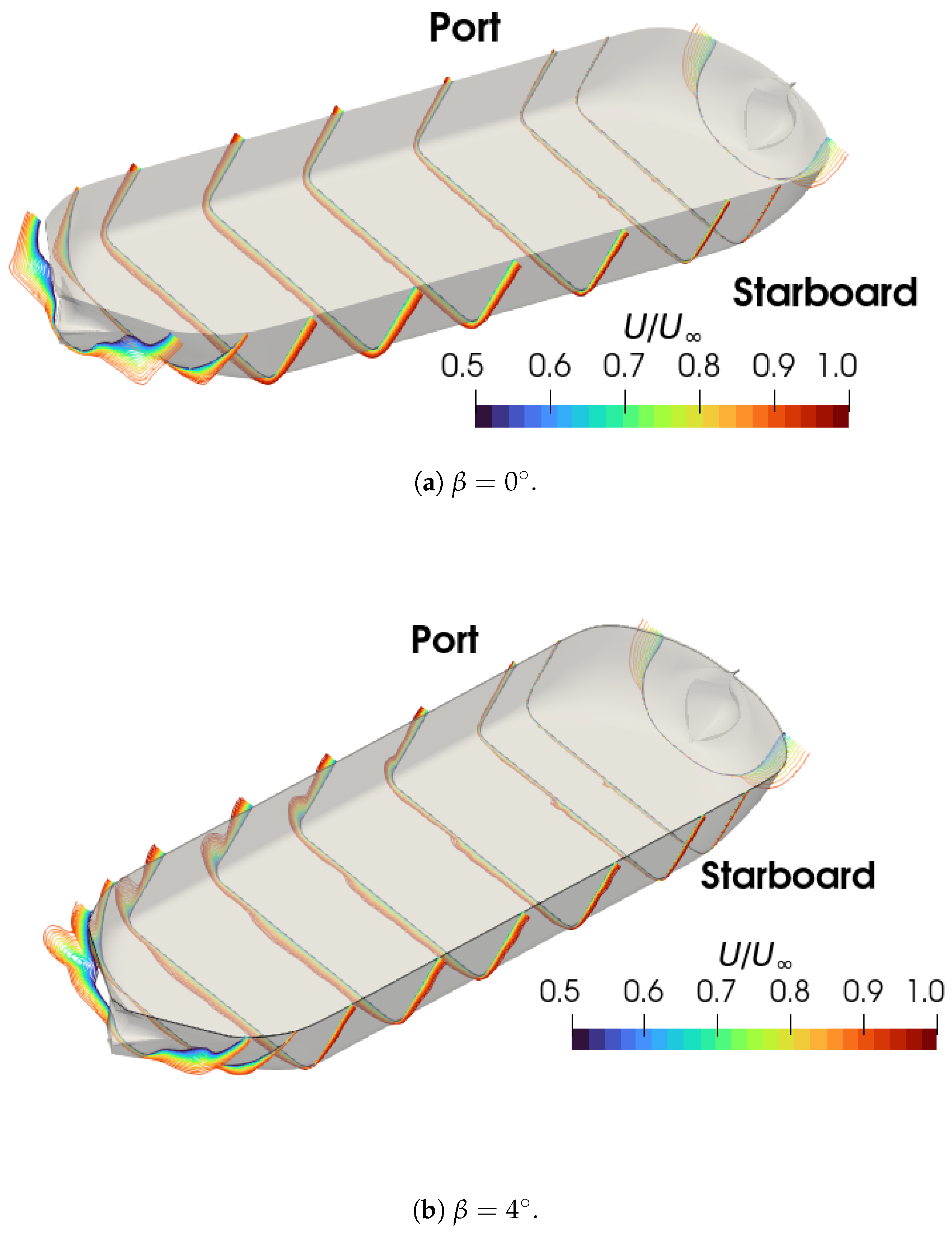
On straight-ahead conditions, Figure 13a, the hull’s pressure distribution is symmetric, resulting in a null lateral force and yaw moment, yielding the regression through the zero (in $Y^{\prime }(\beta =0)=0$). As the drift angle increases, a new configuration surges, the so-called static drift test. In oblique flows in which the drift angle is positive, the stagnation point moves towards the starboard. The flow decelerated in the bow region, and as the velocity dropped, a high-pressure region arose in the fore of the hull. An asymmetric pressure distribution around the hull emerges, leading to a lateral force and yaw moment. At very small angles, $\beta \le 4^{\circ }$, the asymmetry is very smooth, and no perceptible vortices are distinguished, at least to the mesh resolution employed and the turbulence model technique chosen. As seen in Figure 13b, the major asymmetry in the flow occurs in the stern on the port side. Recapitulating the forces computed in these angles, the quantities were low and showed an almost linear behavior. In spite of that, as the drift angle increases, the vortices start to develop on the port side, and as the drift angle approaches 10 degrees (Figure 13c), the vortices become stronger.

4.3.2. Linear Derivatives of Slender Bodies

The KCS container ship analysis revealed that the linear sway derivative ($Y_V^{\prime }$) was underpredicted by the numerical method relative to the linear fit of the experimental data, especially as $\beta$ increased towards ${10}^{\circ }$ (Figure 14). Given the small amount of data to compare the raw data related to the lateral forces, this discussion will be divided into three parts to cover the three angles plotted, referred to as EFD (excluding the point at $\beta =0^{\circ }$). The computed $Y^{\prime }$ at a low angle ($\beta =3^{\circ }$) shows a fair adhesion with the measured value. But, as the drift approaches $\beta =6^{\circ }$, the results start to get further apart but are still acceptable. While $\beta$ approaches 10 degrees, the numerical result is almost half of the value measured in the experiment. This last point yields an increase in the slope of the regression line and, consequently, in the $Y_V^{\prime }$. On top of this, the regression model using the experimental data had worse performance related to the statistics outputs than its peers, as shown in

Table 6. Summary of the linear regression statistics of KRISO Container Ship (KCS).

				${\mathit{Y}}_{\mathit{V}}^{\prime }$
Case	RM	${\mathit{\beta }}_{\mathit{min}}$	${\mathit{\beta }}_{\mathit{max}}$	${\mathit{Y}}_{\mathit{V}}^{\prime }$	${\mathit{R}}^{\mathbf{2}}$	$\mathit{SE}$	$\mathit{p}$
01-CFD	L	0	8	0.123	0.996	0.004	0.000
02-CFD	L	0	12	0.135	0.994	0.004	0.000
03-EFD	L	0	9	0.223	0.972	0.022	0.002
04-EFD	NL	0	18	0.118	0.998	0.002	NP

Note: The column name $RM$ describes the order of the regression model; in this, L stands for linear, and $NL$ denotes nonlinear fitting. Experimental data were taken from [38]. The nonlinear results (derivatives and statics) were taken directly from the SIMMAN report, and the $p$-value was not provided (NP). Meanwhile, the linear regression was obtained using the experimental data points.

. This case is referred to as EFD-linear and was conducted in the context of this study by employing the data provided in the SIMMAN workshop. An alternative analysis of the experimental data is also shown in the table. These results were taken directly from the report, including the statistics.

However, when comparing the 01-CFD linear result ($Y_V^{\prime }$ = 0.123) with $\beta \in [0^{\circ },8^{\circ }]$ to the nonlinear fit 04-EFD/NL ($Y_V^{\prime }$ = 0.118) provided by [38], in which the linear and nonlinear components were adequately accommodated in their respective derivatives, excellent agreement was observed (Table 6). This fact confirms that the numerical method accurately captures the linear component when the range is appropriately selected, and that applying a standard linear fit to highly nonlinear experimental data can severely overestimate the true linear derivative (03-EFD/Linear). Due to observed discrepancies and flow development, the angle limit for linear derivative calculation for slender bodies was reduced to $8^{\circ }$.

4.3.3. Hydrodynamic Coefficients Dependence on the Hull Shape

Figure 15 presents the numerical results obtained in this research and employed to derive the linear derivatives through linear regression, in which the slope represents the ($X_V^{\prime }$), ($Y_V^{\prime }$), and ($N_V^{\prime }$). Additionally, the velocity contours at the same drift angle ($\beta$ = ${10}^{\circ }$) for the two types of vessels previously explored are illustrated. The assumption of linearity is statistically valid within a specified range of drift angles, and this must be discussed in the context of hydrodynamics. For blunt bodies, it was argued that a threshold of 10 degrees is sufficient to capture the required phenomenon. Meanwhile, for slender hulls, this angle should be dropped to 8 degrees.

As shown in the figure, the flow around two different hulls is quite distinct, leading to a greater difference in lateral force. These findings align with the theory that those with a protruding bow show a lower linear sway velocity derivative, whereas those with a shrink bow experience larger lateral forces. Concerning the flow, stronger bilge vortices can be seen in the blunt hull aft, while for the slender ship, the bow vortex can be readily observed, and the stern vortices are relatively weak. As suspected, the shape will significantly affect the linear derivatives, especially the lateral component.

4.4. Validation Against Benchmark Cases

As suggested by [60], the linear derivatives must be validated against benchmark cases. To validate the numerically derived derivatives, four benchmark hulls (Esso Osaka, KVLCC2, S-175, and KCS) with existing experimental data (EFD) were utilized (

Table 7. Overview of the available experimental data of the linear derivatives.

Institute		Type	Model	$\mathit{\lambda }$	${\mathit{F}}_{\mathit{r}}$	$\mathit{\beta }$ Range or ${\mathit{Y}}_{\mathit{v}}^{\prime }$
Esso Osaka
ITTC [37]		CMT	H + R + P	130	0.091	$Y_v^{\prime }=0.383$
KVLCC2
Quadvlieg and Stern [38]	HMRI	PMM	H + R + P	46	0.142	$-2^{\circ }$ to ${16}^{\circ }$
Kume et al. [56]	NMRI	OTT	H	64	0.142	$-3^{\circ }$ to ${18}^{\circ }$
S-175
Son and Nomoto [20]			H + R	58	0.091	$Y_v^{\prime }=0.213$
KCS
Quadvlieg and Stern [38]	JMU	CMT	H + R	105	0.215	$0^{\circ }$ to ${18}^{\circ }$
Quadvlieg and Stern [38]	MARIN	RAT	H + R	37	0.097	$0^{\circ }$ to ${16}^{\circ }$

Notes: In this, the column type brings the type of facility employed to conduct the experiments. The acronym CMT stands for circular motion test, RAT means rotating arm test, and $\lambda$ is the model scale. In the model column, H means that only the hull was considered. Conversely, R and P stand for rudder and propeller, respectively.

). Only the linear derivatives were available for the Esso Osaka and S-175 hulls. On the other hand, for the KVLCC and KCS, two sets of experimental data were available, allowing comparison on the Froude number and related to the influence of appendices (propeller and rudder) on the derivatives. All experiments were restricted to surge, sway, yaw, and roll motions, while heave and pitch were kept unconstrained. The numerical approach, on the other hand, relied on a captive model. Extrapolation to full-scale maneuvering predictions relies on Froude similarity, and the computations were performed at the model scale. Indeed, ref. [5] stated that the scale effects are diminished for the linear component ($Y_V^{\prime }$). Conversely, the cross-drag coefficient has been shown to be more reliant on the Reynolds number.

The numerical results were validated against the analytical and empirical formulations outlined in Section 2.2, with a summary of all findings presented in

Table 8. Validation of the linear sway velocity derivative ($Y_V^{\prime }$).

	Esso Osaka	KVLCC2	S-175	KCS
Benchmark derivative (EFD)	0.383	0.271	0.213	0.119
Numerical method (CFD)	0.382	0.276	0.223	0.117
$E_{rel}[\%]$	−0.313	1.770	4.695	−1.095
Low aspect ratio	0.210	0.204	0.171	0.148
$E_{rel}[\%]$	−45.171	−24.704	−19.933	24.278
Jacobs [12]	0.230	0.220	0.186	0.158
$E_{rel}[\%]$	−39.950	−18.804	−12.890	32.703
Smitt [32]	0.334	0.325	0.271	0.235
$E_{rel}[\%]$	−12.821	19.721	27.307	97.602
Norrbin [16]	0.366	0.357	0.295	0.257
$E_{rel}[\%]$	−4.508	31.580	38.432	116.211
Inoue et al. [19]	0.400	0.410	0.287	0.276
$E_{rel}[\%]$	4.353	51.066	34.636	132.433
Clarke et al. [33]	0.380	0.389	0.275	0.263
$E_{rel}[\%]$	−0.719	43.307	29.048	121.358
Ho-Young Lee et al. [34]	0.323	0.308	0.355	0.328
$E_{rel}[\%]$	−15.751	13.467	66.710	175.959

. For each of the four benchmark hulls, the CFD method consistently produced the lowest percent relative error ($E_{rel}$) for $Y_V^{\prime }$. The relative errors typically remained below $5\%$, whereas empirical methods frequently yielded errors exceeding $100\%$ for slender hulls; for instance, a notable $132.433\%$ for the KCS using [19]. For all these methods evaluated, the percent relative error will be estimated following the formulation given by

$$E_{rel}={\displaystyle \frac{Y_{predicted}^{\prime }-Y_{EFD}^{\prime }}{Y_{EFD}^{\prime }}}·100\%,$$

(12)

where $Y_{EFD}^{\prime }$ will be assumed as the true value, and the experimental method to measure them is explained in Table 7.

Among these methods, the numerical approach proved most effective at estimating the $Y_V^{\prime }$ for the four ship designs under consideration. This outcome underscores the significance of numerical techniques in enhancing maneuvering predictions. Nonetheless, in the daily routine of a ship maneuvering simulator, even with the accuracy of the hydrodynamic coefficient sought, it may sometimes be unsuitable due to time limitations. Although the numerical method has proven efficient in yielding rapid results, the task of obtaining the required derivatives continues to be time-consuming. Even though the numerical method has proven efficient at providing results quickly, obtaining derivatives remains a time-consuming task. Between pre-processing and delivery, the $Y_V^{\prime }$ prediction will take around 130 h It was estimated that the pre-processing phase would take 40 h, followed by 60 h to compute results at six different drift angles and more than 30 h to post-process the results and apply the regression model. and require the ship’s geometry.

As previously mentioned, empirical methods have been found to produce miscalculations in $Y_V^{\prime }$ predictions, primarily because many of these formulations were developed using data from older ship designs. Moreover, some methods relied exclusively on ships with high block coefficients ($C_B$), raising questions about their applicability to slender vessels. In light of this, the next section will focus on developing a regression formula to predict the linear derivative $Y_V^{\prime }$.

5. Regression Model to Predict the Linear Sway Velocity Derivative

Once the hydrodynamic forces and linear derivatives have been validated through a series of virtual static drift tests, followed by linear regression analysis to obtain $Y_V^{\prime }$, the results are corroborated by experimental data. This section now focuses on validating standard ship maneuvers. In particular, an empirical formulation is introduced to estimate the linear sway velocity derivative ($Y_V^{\prime }$) based on the vessel’s principal dimensions. To ensure its precision, the maneuvering parameters obtained from both the numerical approach (CFD) and the newly developed empirical formulation will be validated by performing standard maneuvers within a mathematical model. The $Y_V^{\prime }$ values derived from both methodologies will then be compared with experimental results.

5.1. Systematic Hull Series Generation Using Grasshopper

A significant challenge in CFD-based virtual model testing is the availability of reliable, easily modifiable hull geometries. To overcome this, a parametric model was developed using Grasshopper, a Rhino plugin that allows the creation of graphical algorithms (see [61] for more details), allowing systematic modification of hull shapes based on a parent hull.

The process utilizes an available ship body plan and main dimensions to construct a reference model. The workflow includes digitalization of the body plan, manual acquisition of characteristic points, modification of these points via dedicated Python 3.12.4 scripts to parametrize variables (

Table 9. Parametrization model parameters on Grasshopper.

Variable	Description
Length $\%L_{PP}$	The length may vary as a function of the reference dimension, typically the one related to the parent hull.
Beam $\%B$	The beam will vary with the reference value, which is typically associated with the parent hull input.
Draft T	The draft must be ascertained by the user.
Bilge radius $\%bilge$	By changing the percentage of the bilge radius, the station’s curvature will be modified. This parameter will most affect the block coefficient. The user can choose which stations should be modified.

), automatic reconstruction of station curves, computation of hydrostatics, and exporting the geometry as a mesh (.STL) file for CFD simulation.

Key parameters systematically varied in the model include the main dimensions (length, beam, draft), bilge radius, and contributions from the bow and stern regions. The bow parametrization follows the nomenclature provided by [62], varying width, length, and height (Figure 16). Additionally, stern variations were included, such as the curvature of the stern frame and transom length.

5.2. Modern Hull Database

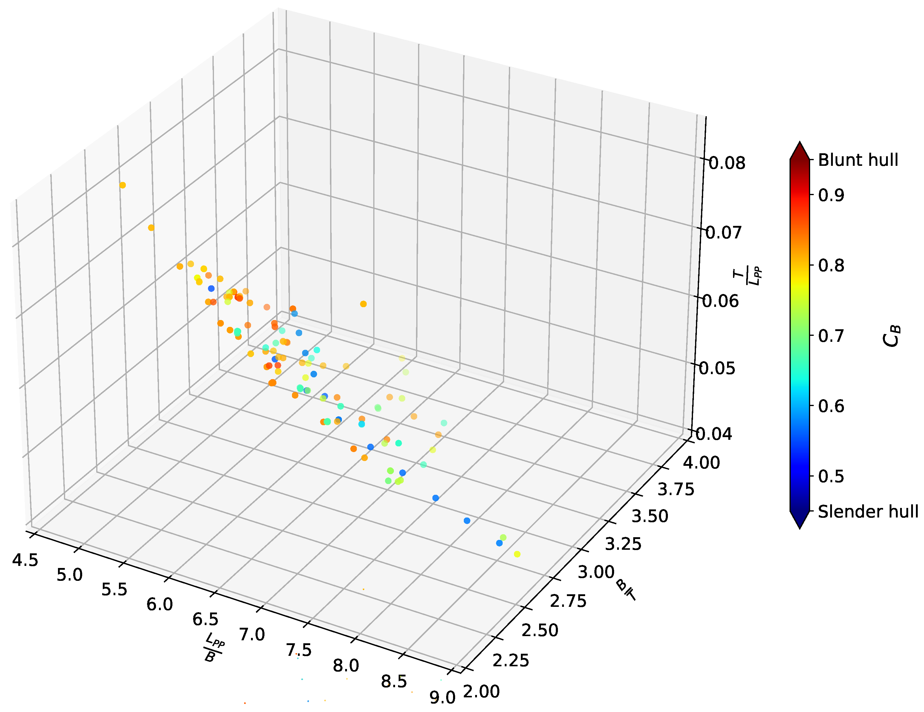
Drawing upon identified changes in ship design over recent decades (increased size, decreased non-dimensional parameter $C_{B}B/T$, prevalence of bulbous bows/sterns), a database was constructed using seven reference parent hulls. By systematically varying these geometric references, a total of 115 distinct hull geometries were generated. The hydrostatic characteristics of these hulls were calculated and used as predictors in subsequent regression analysis, along with the main dimensions. The database covers a wide range of non-dimensional geometric coefficients, as summarized in

Table 10. Range of applicability of the proposed regression formula.

	Type of Ship	${\mathbf{L}}_{\mathbf{PP}}/\mathbf{B}$	$\mathbf{B}/\mathbf{T}$	$\mathbf{T}/{\mathbf{L}}_{\mathbf{PP}}$	${\mathbf{C}}_{\mathbf{B}}$
RM database	T, CS	4.91–8.80	2.30–3.98	0.041–0.083	0.552–0.877
MH database	T, BC, CS	5.26–8.78	2.22–3.81	0.042–0.071	0.614–0.888

Notes: $RM$ corresponds to those geometries used as the database in the regression model, while $MH$ indicates the modern hull database. The ship’s type was divided into three categories: tankers (T), bulk carriers ($BK$), and containerships ($CS$).

and visualized in Figure 17.

5.3. Regression Model

The objective of this stage was to derive an empirical expression that describes the behavior of the linear sway derivative ($Y_v^{\prime }$) as a function of the ship form parameters. The data acquisition process involved conducting 690 virtual static-drift tests (see Section 3) across 115 hull designs generated by the Grasshopper code (see Section 5.1). Computations were performed for drift angles ranging from $0^{\circ }$ to ${10}^{\circ }$ for tankers and from $0^{\circ }$ to $8^{\circ }$ for containerships, with increments of $2^{\circ }$. A linear regression model (see Section 4) was applied to each hull, resulting in 115 distinct $Y_v^{\prime }$ values.

A preliminary regression analysis, following principles outlined by [63], was conducted to identify the most suitable geometric predictors for $Y_v^{\prime }$. As shown in

Table 11. Summary of the regression results for different predictors.

Variable	${\mathit{R}}^2$	SE	$\mathit{p}\text{-}\mathit{Test}$
$C_{B}B/T$	0.373	1.135	0.000
$C_{B}B/L$	0.507	0.151	0.000
$C_{B}T/B$	0.883	0.053	0.000

, the predictor $C_{B}T/B$ demonstrated the strongest correlation, exhibiting an $R^2$ value of 0.883 and the lowest standard error ($\mathrm{SE}=0.053$). Consequently, $C_{B}T/B$ was selected as the primary variable to build the regression model.

5.4. Empirical Formula to Predict Linear Sway Velocity Derivative ($Y_V^{\prime }$)

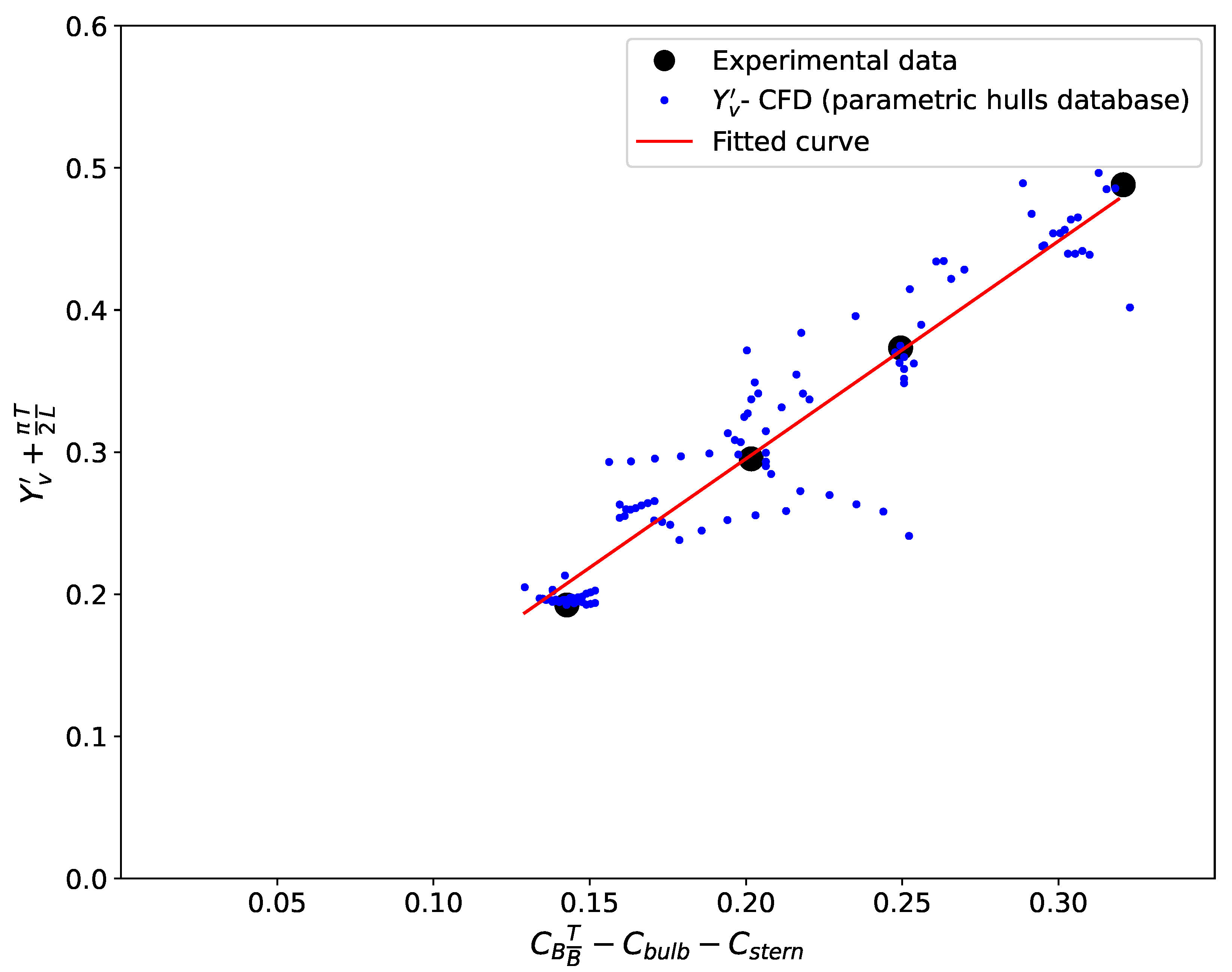
The graphical representation of this regression model is presented in Figure 18. It is important to note the composition of the axes: the dependent variable (y-axis) incorporates a term related to the low aspect ratio wing theory, added to the ${\mathrm{Y}}_V^{\prime }$ derivative. The predictor term (x-axis), conversely, is composed of three distinct components: one representing a non-dimensional geometric parameter of the hull form, with the remaining two accounting for the specific influences of the bow and stern shapes, respectively.

To enhance the model’s accuracy, particularly for modern designs, the influence of bow and stern geometries was incorporated via dedicated coefficients. The bow coefficient ($C_{bow}$) (Equations (13) and (14)) captures the impact of a bulbous bow, where its absence or type (blunt/slender hull) suggests default values. The stern coefficient ($C_{stern}$) (Equation (15)) accounts for stern frame shape (flat, U-shape, or V-shape).

$$C_{bow}=\sqrt{C_{lb}{C}_{wb}{C}_{hb}}\left\{\begin{array}{c}\mathrm{No}\mathrm{bulbous}\mathrm{bow},C_{bow}=0.015\hfill \\ \mathrm{Blunt}\mathrm{hull}\mathrm{w}/\mathrm{bulbous}\mathrm{bow},C_{bow}=0.03\hfill \\ \mathrm{Slender}\mathrm{hull}\mathrm{w}/\mathrm{bulbous}\mathrm{bow},C_{bow}=0.045\hfill \end{array}\right.$$

(13)

$$C_{lb}={\displaystyle \frac{L_{bulbous}}{L_{PP}}},C_{wb}={\displaystyle \frac{B_{bulbous}}{B}},C_{hb}={\displaystyle \frac{H_{bulbous}}{T}}$$

(14)

$$C_{stern}=C_{frame}{\displaystyle \frac{\frac{T}{L_{PP}}}{{(L_{WL}-L_{PP})}^2}}\left\{\begin{array}{c}\mathrm{if}\mathrm{flat},C_{frame}=0\hfill \\ \mathrm{if}\mathrm{U}\text{-}\mathrm{shape},C_{frame}=1\hfill \\ \mathrm{if}\mathrm{V}\text{-}\mathrm{shape},C_{frame}=0.9\hfill \end{array}\right.$$

(15)

If the parameter $L_{WL}$ is unavailable (or unknown), the following value can be used as an estimate

$$C_{stern}=\left\{\begin{array}{c}\mathrm{if}\mathrm{old}\mathrm{design},C_{stern}=0\hfill \\ \mathrm{if}\mathrm{modern}\mathrm{hull},C_{stern}=0.005\hfill \end{array}\right.$$

(16)

By rearranging the terms and incorporating the constant, which represents the slope derived from the linear regression analysis, the final empirical formulation is obtained as follows

$$Y_v^{\prime }=1.53\left(C_B{\displaystyle \frac{T}{B}}-C_{bow}-C_{stern}\right)-{\displaystyle \frac{\pi }{2}}{\displaystyle \frac{T}{L_{PP}}}·$$

(17)

5.5. Case Study—Assessment of the Range of Applicability Against the PIANC Reference Fleet

The geometric validity and range of applicability of the proposed formulation were assessed against a comprehensive vessel database provided in Appendix A of the PIANC MarCom Working Group Report N° 235 [64]. This report serves as an industry guideline, offering dimensions and characteristics for ocean-going vessels by type and size, including detailed data on Length Overall ($L_{OA}$), Length Between Perpendiculars ($L_{PP}$), Beam (B), Draft (T), and Block Coefficient ($C_b$).

The analysis evaluated whether the geometric properties of these vessels fall within the valid range of the proposed formula, as defined in Table 10. This verification was performed for both “Upper” (maximum expected) and “Typical” (mean) dimensional values for each ship class, the average block coefficient ($C_b$) value was adopted as suggested by PIANC. The results are summarized in

Table 12. Analysis of the range of applicability for various ship types [64]. The Upper column denotes the maximum value for the respective class of the maind dimension parameters. The symbols ✓ and × indicate whether the ship parameters are within or outside the valid range of the formula, respectively.

Ship Type	DWT (t)	Class	Upper	Typical
Bulk Carriers	400,000	Chinamax	✓	✓
	325,000	VLOC	✓	✓
	300,000	VLOC	✓	✓
	250,000	VLOC	✓	✓
	230,000	Large Cape	✓	✓
	200,000	Cape	✓	✓
	185,000	Cape	✓	✓
	170,000	Cape	✓	✓
	150,000	Small Cape	✓	✓
	120,000	Mini Cape	✓	✓
	100,000	Post Panamax (wide)	✓	✓
	100,000	Post Panamax (narrow)	✓	✓
	85,000	Post Panamax	✓	✓
	80,000	Panamax	×	×
	70,000	Panamax	✓	✓
	60,000	Supramax	✓	✓
	50,000	Handymax	✓	✓
	40,000	Handymax	✓	✓
	30,000	Handy size	✓	✓
	20,000	Handy size	✓	✓
	10,000	Handy size	✓	✓
	5000	-	✓	✓
Container Ships	65,000	-	✓	✓
(Panamax & smaller)	60,000	-	✓	✓
	55,000	-	✓	✓
	50,000	-	✓	✓
	45,000	-	✓	✓
	40,000	-	✓	✓
	35,000	-	✓	✓
	30,000	-	✓	✓
	25,000	-	✓	✓
	20,000	-	✓	✓
	15,000	-	✓	✓
	10,000	-	✓	✓
Container Ships	240,000	-	✓	✓
(Post-Panamax)	225,000	-	✓	✓
	200,000	-	✓	✓
	185,000	-	✓	✓
	165,000	-	✓	✓
	150,000	-	✓	✓
	130,000	-	✓	✓
	120,000	-	✓	✓
	110,000	-	✓	✓
	100,000	-	✓	✓
	90,000	-	✓	✓
	80,000	-	✓	✓
	70,000	-	✓	✓
	65,000	-	✓	✓
	60,000	-	✓	✓
	52,000	-	✓	✓
Crude oil tankers	450,000	ULCC	✓	✓
	320,000	VLCC	✓	✓
	300,000	VLCC	✓	✓
	280,000	VLCC	✓	✓
	193,000	VLCC	✓	✓
	165,000	VLCC	✓	✓
	150,000	Suezmax	✓	✓
	115,000	Aframax	✓	✓
	100,000	Aframax	✓	✓
	70,000	Coastal/Panamax	✓	✓
	60,000	Coastal/Panamax	✓	✓
General Cargo Vessels	55,000	-	✓	✓
	50,000	-	✓	✓
	45,000	-	✓	✓
	38,000	-	✓	✓
	35,000	-	✓	✓
	30,000	-	✓	✓
	25,000	-	✓	✓
	18,000	-	✓	×
	10,000	-	✓	×
	5000	-	✓	✓
	2500	-	✓	✓
LNG	155,000	LNG-QMax	×	×
	130,000	LNG-QMax	×	×
	120,000	LNG-Qflex	✓	✓
	107,000	LNG-Qflex	×	×
	98,000	LNG New Panamax	✓	✓
	90,000	LNG New Panamax	✓	✓
	80,000	LNG Conventional	✓	✓
	70,000	LNG Conventional	✓	×
	40,000	LNG Conventional	✓	✓
	20,000	Combination Gas/LPG	✓	✓
	11,000	LNG Small
	10,000	Combination Gas/LPG	✓	✓

and demonstrate a high degree of applicability across the majority of the commercial fleet.

Regarding specific ship types, the formulation is applicable to nearly all standard sizes of bulk carriers and tankers, ranging from Handysize to ULCCs. A single exception was observed for the 80,000 DWT Panamax bulk carrier, which falls outside the applicability range in both upper and typical scenarios. Similarly, the formula is applicable to all the container ships analyzed, covering the full spectrum from small feeders (10,000 DWT) to ultra-large Post-Panamax vessels (240,000 DWT).

While most general cargo vessels are covered, a divergence appears in the mid-range sizes (10,000 to 18,000 DWT). These vessels fit the criteria under “Upper” dimensions but fail under “Typical” dimensions, suggesting that the average hull form for these specific sizes possesses ratios (such as $L/B$ or $B/T$) that are borderline for the proposed method. Conversely, LNG carriers show the most significant limitations. Large Q-Max (130k–155k DWT) and some Q-Flex vessels consistently fall outside the valid range. Additionally, the 70,000 DWT conventional carrier is applicable only under its upper dimensional limits. This is likely due to the unique volumetric constraints and shallower draft characteristics of gas carriers compared to displacement-heavy vessels like tankers. This analysis sheds light on a critical aspect of the proposed formula: applicability is highly dependent on the draft (loading condition). The excellent agreement observed for tankers and container ships is a consequence of the fact that the underlying database used to derive the regression model consisted primarily of loaded vessels. Therefore, since LNG vessels were not included in the derivation database and frequently fall outside the geometric limits, their use with this formulation should be avoided.

5.5.1. Constraints and Recommendations

To apply the proposed formula, the vessel must first satisfy the following geometric criteria:

• $4.91<L/B<8.80$
• $2.30<B/T<3.98$
• $0.041<T/L<0.083$
• $0.55<C_b<0.88$

Even if a ship falls within the geometric criteria above, the following operational and modeling restrictions are advised:

1.

Loading Condition: The formula should be applied with caution in ballast conditions, given the majority of the database employed was composed of loaded hull data.

2.

Ship Type Extension: While derived specifically from tankers and container ships, the method can be extended to general cargo vessels and bulk carriers with caution, due to their similar hull characteristics.

3.

Flow restrictions: The static drift tests were performed at a low-speed regime ($Fr<0.2$) and deep-water conditions; the formula is strictly valid under these specific conditions.

4.

Appendages: The linear derivative in the present research was obtained for a bare hull. This differs from some mathematical models where the lateral velocity derivative implicitly accounts for the rudder and propeller. Users must account for this distinction.

5.

Linearity and Drift Angle: The regression model is built on the premise of small angles to guarantee linearity (as discussed in Section 4.3). Consequently, the formula will reasonably represent the linear counterpart of the lateral force In the in-house mathematical model used herein, the non-linear component of the lateral force (Equation (11)) is treated separately based on cross-flow drag theory. Therefore, the validity threshold for this linear formulation is estimated at 10 degrees for blunt bodies and 8 degrees for slender hulls.

6.

Hull Form Parameterization: The formulation is designed to accommodate varying levels of input data detail. Specifically:

• Bulbous Bow: While the inclusion of specific bulb dimensions yields a more precise hydrodynamic description, the user may resort to suggested reference values for three bulbous bow types (Equation (13)) if detailed data is lacking.
• Stern Profile: The afterbody geometry can be characterized through simple visual assessment of the stern type (distinguishing between U-shaped or V-shaped sections). Alternatively, if this specific information is unavailable, the formulation remains robust through the use of standard reference values for the stern coefficient ($C_{stern}$) based on the design of the hull (old or modern).

In summary, as exemplified in this section, the proposed method covers a wide spectrum of merchant vessel classes but must be applied with due attention to these established constraints.

5.5.2. Open-Source Toolkit

As a means of demonstrating the operational use of the proposed method, a simplified algorithm developed in Python is available (on github). This algorithm exemplifies the calculation procedure utilizing default reference values for both $C_{stern}$ and $C_{bow}$, ensuring applicability even when detailed hull form coefficients are not explicitly known.

To facilitate the application of the proposed formulation and ensure reproducibility, a computational tool was developed in Python. This script, which includes the automatic verification of the range of applicability and the hull form coefficient estimation, is available as supplementary material. The code is available at [65].

The algorithm verifies if the vessel’s geometry is within the range of applicability used to derive the formula. If any parameter is out of bounds, the vessel is flagged as “Not Applicable,” though the calculation proceeds for comparison purposes. Additionally, a draft sensitivity analysis is performed as a specific subroutine that calculates the valid range of draft (T) for the given length and beam. It determines the intersection of constraints imposed by the $B/T$ and $T/L$ limits. Such analysis was included based on the discussion above.

5.6. Comparison with Available Data

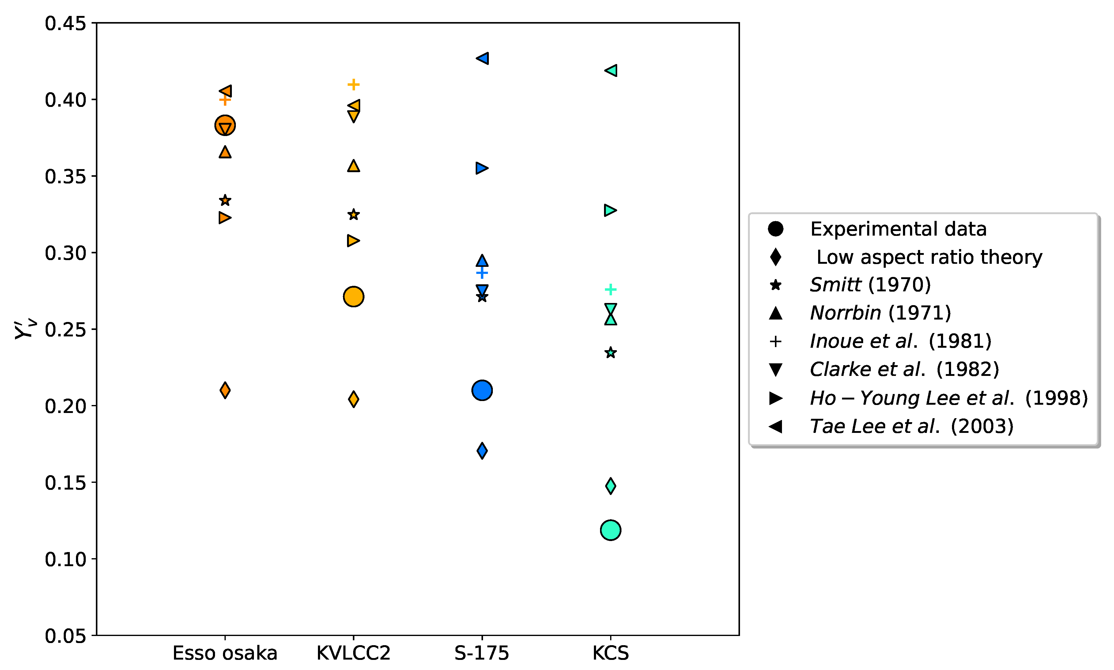
The proposed formula (Equation (17)) was tested against experimental data, numerical results, and existing empirical methods for seven reference ships (Figure 19).

For the four benchmark cases possessing experimental data (Esso Osaka, S-175, KVLCC2, and KCS), the absolute relative error of the new formula ranged from $1.15\%$ to $18.03\%$. This significantly outperforms other conventional empirical methods, which yielded relative errors between $4.35\%$ and $176\%$, confirming that the goal of improving $Y_v^{\prime }$ prediction for both modern and older hull forms was achieved.

5.7. Validation of Maneuvering Trajectories

The validation of maneuvering simulation models relies on a rigorous, interconnected procedure, as established by the ITTC [60]. As illustrated in the adapted diagram (Figure 20), deficiencies in the prediction of fundamental hydrodynamic forces (e.g., lateral force and yaw moment) cascade into inaccuracies in linear derivative and trajectory validation. A survey among maneuvering organizations revealed that most institutes prioritize validation against benchmark data, mirroring the approach adopted in this study. Key validation stages include comparing results against virtual free-running data (a method utilized by $36\%$ of institutions) and comparing simulated trajectories against physical free-running tests ($61\%$ of institutions). Three primary validation steps were executed, excluding real-time simulation, to evaluate the mathematical model and the novel regression formulation for hydrodynamic coefficients.

Fast-time simulations were conducted employing the Numerical Offshore Tank Mathematical Model (MM-TPN). The KVLCC2 tanker was selected for these tests due to the availability of benchmark data (

Table 13. Main characteristics of the KVLCC2.

Main Dimensions	Value	Unit
Length between perpendicular (LPP)	320	[m]
Beam (B)	58	[m]
Draft (T)	20.8	[m]
Metacentric height (GM)	5.71	[m]
Ship’s speed	15.5	[knots]
Rudder and propeller characteristics	Value	Unit
Mean chord	7.8	[m]
Rudder height	15.8	[m]
Rudder rate of turn	2.32	[deg/s]
Propeller diameter	9.86	[m]
Maneuvering coefficients	Value	Description
$C_0^{\prime }$	0.01634	ITTC correlation line [36]
$C_Y$	0.76	Hoerner’s curve
$l{C}_Y$	0.035	Typical value for tanks

). Two sets of simulations were performed: one using the $Y_v^{\prime }$ derived from the novel empirical formula (Equation (17)) and a second using the coefficient provided by Clarke’s traditional formulation.

5.7.1. Turning Circle Maneuver

A turning maneuver can be conceptually split into transient and steady components, from which distinguishing characteristics are derived. A ship in a steady turn, typically achieved after approximately ${270}^{\circ }$ of heading change, yields a crucial measurement known as the Steady Turning Diameter (STD), which is directly related to the vessel’s stability. A ${35}^{\circ }$ turning circle maneuver was simulated for KVLCC2 (Figure 21).

Table 14. Turning circle maneuver characteristics and average error per method.

Method Employed to Determined ${\mathit{Y}}_{\mathit{V}}^{\prime }$	$\mathbf{AD}/\mathit{L}$	$\mathbf{TC}/\mathit{L}$	$\mathit{V}/{\mathit{V}}_0$	${\mathit{R}}_{\mathit{C}}/\mathit{L}$	$\mathit{r}{\mathit{c}}^{\prime }$	${\mathit{\beta }}_{\mathit{c}}$	$\overline{\left|{\mathit{E}}_{\mathbf{rel}}[\%]\right|}$
Benchmark data (SIMMAN’20)	3.02	3.04	0.36	1.23	0.81	20.2	-
Analytical method (ABS, 2017)	2.82	2.88	-	1.013	-	-	-
$E_{rel}[\%]$	−6.62	−5.26	-	−17.64	-	-	-
Empirical proposed in this work	2.86	3.31	0.36	1.16	0.86	24.5	-
$E_{rel}[\%]$	−5.29	−8.81	0.0	−5.69	6.17	21.29	-
Average error per method							7.88
Empirical proposed by Clarke	3.10	3.77	0.42	1.34	0.75	19.9	-
$E_{rel}[\%]$	2.65	24.01	16.66	8.94	−7.41	−1.48	-
Average error per method							10.19

bring a comparison on the turning characteristics of the empirical proposed method against benchmark data (SIMMAN’20), an analytical method (Lyster regression [66]), and Clarke’s empirical method.

A comparison against SIMMAN’20 benchmark data demonstrated the quality of the newly proposed empirical method for $Y_V^{\prime }$. This method yielded an average relative error ($\overline{\left|E_{rel}[\%]\right|}$) of $7.88\%$, lower than the $10.19\%$ error observed using the coefficients derived from Clarke’s formulation. The analytical method tended to underestimate turning variables, particularly the steady turning radius, which has implications for stability assessment.

5.7.2. Zigzag Maneuver

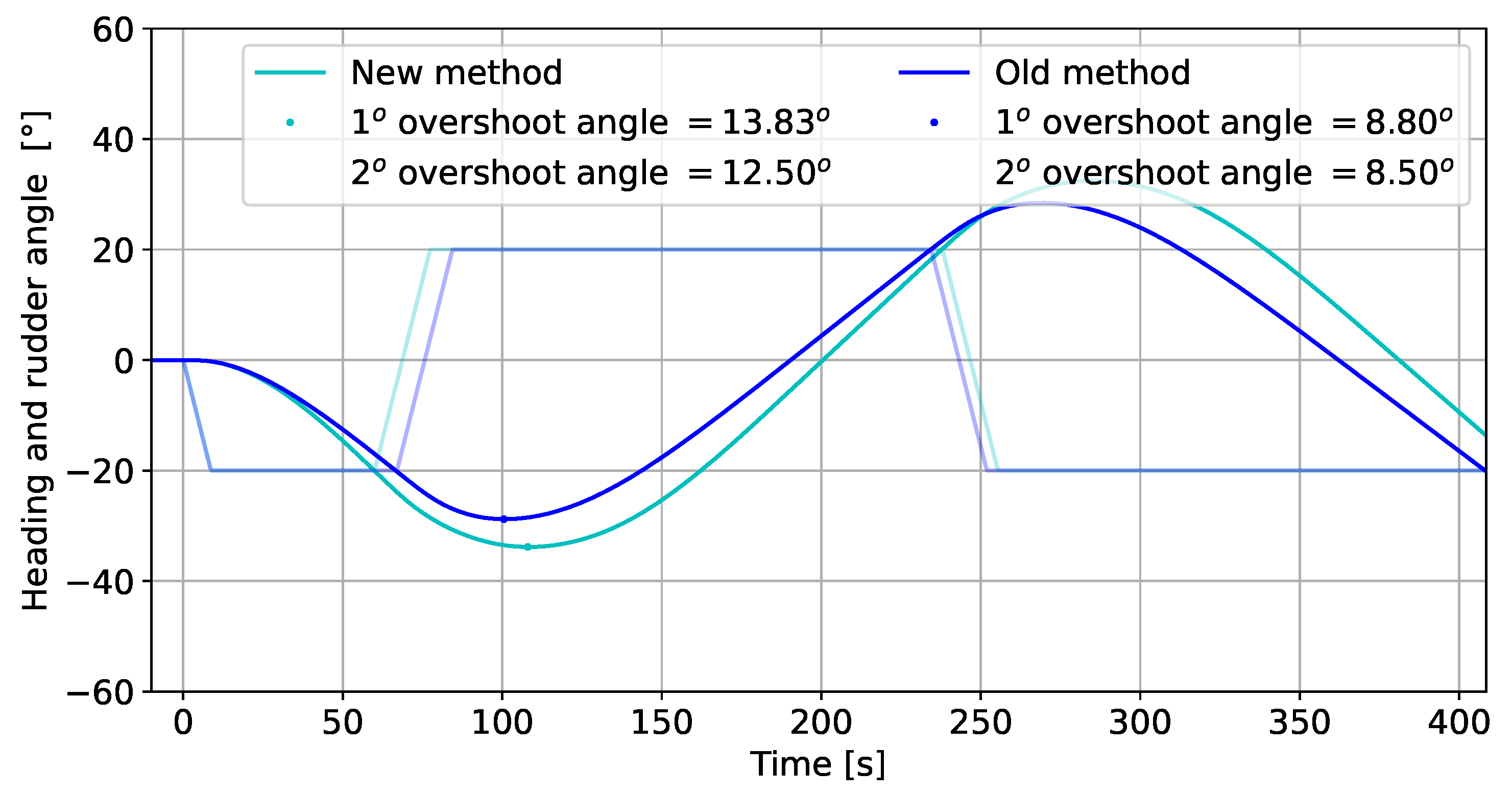
The ${20}^{\circ }/{20}^{\circ }$ zigzag maneuver, which assesses ship handling qualities (Figure 22), revealed that the accurate prediction of the linear derivative $Y_v$ is essential. The traditional method severely underestimated the first overshoot angle ($OV{A}_1$) by over $35\%$, leading to misleading on the maneuvering predictions (

Table 15. Zigzag maneuver characteristics and average error per method.

Method Employed to Determined ${\mathit{Y}}_{\mathit{V}}^{\prime }$	${\mathit{OVA}}_1$	${\mathit{OVA}}_2$	$\mathit{ITA}$	${\mathit{T}}_{1/2}$	${\mathit{r}}_{\mathit{max},1}^{\prime }$	${\mathit{r}}_{\mathit{max},2}^{\prime }$	$\overline{\left|{\mathit{E}}_{\mathit{rel}}[\%]\right|}$
Benchmark data (SIMMAN’20)	13.08	14.9	1.85	5.3	0.36	0.44	-
Empirical proposed in this work	13.83	12.5	1.52	4.5	0.4	0.44	-
$E_{rel}[\%]$	0.22	−16.1	−17.83	−15.09	11.11	0.0	-
Average error per method							10.06
Empirical proposed by Clarke	8.8	8.5	1.69	4.2	0.32	0.36	-
$E_{rel}[\%]$	−36.23	−42.95	−8.64	−20.75	−11.11	−18.18	-
Average error per method							22.98

).

Using the updated formula resulted in a substantial reduction in the overall average relative error for zigzag characteristics, from $22.98\%$ (Clarke’s method) to $10.06\%$ (new empirical method). This comprehensive validation sequence confirms the reliability of the MM-TPN when coupled with the novel regression formula for $Y_V^{\prime }$. Furthermore, the study highlights the successful deployment of Computational Fluid Dynamics (CFD) to generate systematic data series, thereby replacing expensive physical experiments for deriving empirical formulations.

6. Conclusions

Accurate prediction of lateral forces under oblique flow conditions is critical for determining the linear hydrodynamic derivatives required for ship maneuvering simulations. In this context, a methodology for conducting virtual static drift tests was introduced, and the numerical results were validated against benchmark cases. For the lateral force coefficients, the numerical uncertainty ($U_{SN}$) was maintained below $5\%$ in all test cases. Satisfactory convergence was achieved using meshes comprising approximately four million cells, ensuring computational feasibility.

An extensive discussion was first conducted regarding the regression model employed to obtain the linear derivatives. First, ${\mathrm{Y}}_V^{\prime }$ obtained by the CFD-based method was confronted with benchmark experimental data (provided by the SIMMAN workshop), exhibiting a maximum relative error of only $\mathbf{4.7}\%$, while empirical methods frequently yielded errors exceeding $100\%$ for modern hulls. A significant output from this work is the establishment of critical thresholds for linearity based on hull type: ${\mathbf{10}}^{\circ }$ for blunt hulls and ${\mathbf{8}}^{\circ }$ for slender hulls.

While viscous-flow computation methods can be helpful for estimating the linear sway velocity derivative of a ship, they are limited by the availability of the hull geometry. As such, a semi-empirical approach may be a more practical technique in the context of a ship maneuvering simulator, as it relies solely on the ship’s main dimensions. A significant contribution of this work involves the development of a novel semi-empirical approach specifically designed for scenarios where hull geometry is unknown. A parametric modeling platform (Grasshopper) was employed to generate 115 distinct hull forms systematically. The extensive numerical effort, encompassing 690 virtual static-drift tests, provided the necessary foundation for the development of a novel regression formulation for $Y_V^{\prime }$. This formula represents a significant step forward, as it is derived directly from modern hull geometries and explicitly includes terms related to the bow and stern characteristics.

This novel empirical method demonstrated substantial improvements in predictive accuracy. When validating the overall mathematical model using the Numerical Offshore Tank Mathematical Model (MM-TPN) against experimental standard maneuver trajectories, the proposed method reduced the absolute relative error from $\mathbf{23}\%$ to $\mathbf{10}\%$, when compared with traditional empirical formulations used to feed the mathematical model (such as the MM-TPN). These findings underscore the potential of integrating advanced CFD simulations with regression analysis to enhance safety and reliability in maneuvering operations by providing more precise maneuvering coefficients for ship simulators.

This study successfully implemented a rigorous three-step validation process, focusing on hydrodynamic forces, linear derivatives, and standard maneuvers. The process led to some intriguing conclusions, culminating in a novel approach that is described below.

• The lateral force can be obtained employing a numerical model in CFD (herein using an open-source code called OpenFoam) in less than 24 h and $U_{SN}<5\%$.
• These hydrodynamic forces may be used directly in the mathematical model used to predict maneuvers or as a database to fit a linear regression model and obtain the linear derivatives. In both cases, the hull geometry will be considered when determining the hydrodynamic component.
• Regarding the linear derivatives, some thresholds were established for two different ship types: a blunt hull and a slender one. For the former, the linearity condition is suitable up to 10 degrees; for the slender hull, it should be set at 8 degrees.
• A novel approach to predicting the linear velocity derivative was proposed based only on a ship’s main characteristic. This method is recommended when the geometry is unavailable and the $Y_V^{\prime }$ must be determined.

References

1. Papanikolaou, A.; Zaraphonitis, G.; Bitner-Gregersen, E.; Shigunov, V.; el Moctar, O.; Soares, C.G.; Reddy, D.N.; Sprenger, F. Energy efficient safe ship operation (SHOPERA). In Proceedings of the SNAME Maritime Convention and 5th World Maritime Technology Conference, Providence, RI, USA, 3–7 November 2015. [Google Scholar]
2. Standards for Ship Manoeuvrability. Resolution MSC.137(76)4. Adopted on 04 December 2002. Available online: https://wwwcdn.imo.org/localresources/en/KnowledgeCentre/IndexofIMOResolutions/MSCResolutions/MSC.137(76).pdf (accessed on 10 September 2023).
3. Brix, J. Manoeuvring Technical Manual; Seehafen Verlag: Hamburg, Germany, 1993. [Google Scholar]
4. Brard, R. A Mathematical Introduction to Ship Maneuverability; Technical Report; The David W. Taylor Naval Ship Research and Development Center: Carderock, MD, USA, 1976.
5. Newman, J.N. Some Hydrodynamic Aspects of Ship Maneuverability; Office of Naval Research: Washington, DC, USA, 1966.
6. Davidson, K.S.; Schiff, L.I. Turning and Course Keeping Qualities; Stevens Institute of Technology, Experimental Towing Tank: Hoboken, NJ, USA, 1946. [Google Scholar]
7. Eda, H.; Crane, C.L., Jr. Steering characteristics of ships in calm water and waves. Soc. Nav. Archit. Mar. Eng.-Trans. 1965, 73. Available online: https://trid.trb.org/View/158118 (accessed on 2 December 2025).
8. Strom-Tejsen, J. A Digital Computer Technique for Prediction of Standard Maneuvers of Surface Ships; Technical Report; David Taylor Model Basin, Department of the Navy: Carderock, MD, USA, 1965.
9. Abkowitz, M.A. Lectures on Ship Hydrodynamics–Steering and Manoeuvrability; Technical Report; Hydro and Aerodynamics Laboratory: Lyngby, Denmark, 1964. [Google Scholar]
10. Nomoto, K. Analysis of the ITTC manoeuvrability tests for the mariner type ship in terms of steering quality indices K and T. In Proceedings of the 11th International Towing Tank Conference, ITTC’66: Subject Manoeuvrability, Tokyo, Japan, October 1966; pp. 534–536. Available online: https://trid.trb.org/View/159193 (accessed on 2 December 2025).
11. Jacobs, W.R. Method of predicting course stability and turning qualities of ships. Int. Shipbuild. Prog. 1964, 11, 414–425. [Google Scholar] [CrossRef]
12. Jacobs, W.R. Estimation of Stability Derivatives and Indices of Various Ship Forms, and Comparison with Experimental Results2. J. Ship Res. 1966, 10, 135–163. [Google Scholar] [CrossRef]
13. Motora, S. Manoeuvrability at slow speed. In Proceedings of the 11th International Towing Tank Conference, ITTC’66: Subject Manoeuvrability, Tokyo, Japan, October 1966; pp. 540–542. [Google Scholar]
14. Asinovsky, V.; Landsburg, A.C.; Hagen, G. A Case for the Separate Determination of Hydrodynamic Characteristics of Ship’S Hull And Rudder. In Proceedings of the 21st International Towing Tank Conference, Trondheim, Norway, 15–21 September 1996. [Google Scholar]
15. Crane, C.L., Jr. Studies of Ship Maneuvering ‘Response to Propeller and Rudder Actions’; Technical Report; Stevens Institute of Technology: Hoboken, NJ, USA, 1965. [Google Scholar]
16. Norrbin, N.H. Theory and Observations on the Use of a Mathematical Model for Ship Manoeuvring in Deep and Confined Waters; Technical Report; The Swedish State Shipbuilding Experimental Tank: Gothenburg, Sweden, 1971. [Google Scholar]
17. Santos, E.M. Uma Abordagem sobre Modelos Matemáticos para Simulação de Manobras de Navios em Tempo Real. Master’s Thesis, Universidade Federal do Rio de Janeiro, Rio de Janeiro, Brazil, 1999. [Google Scholar]
18. Ma, C.; Ma, N.; Gu, X. Benchmarking study and uncertainty assessment of planar motion mechanism tests on kvlcc2 in a circulating water channel. In Proceedings of the ASME 2021 40th International Conference on Ocean, Offshore and Arctic Engineering (OMAE2021), Virtually, 21–30 June 2021. Paper No: OMAE2021-62671. [Google Scholar] [CrossRef]
19. Inoue, S.; Hirano, M.; Kijima, K. Hydrodynamic derivatives on ship manoeuvring. Int. Shipbuild. Prog. 1981, 28, 112–125. [Google Scholar] [CrossRef]
20. Son, K.; Nomoto, K. On the coupled motion of steering and rolling of a high speed container ship. J. Soc. Nav. Archit. Jpn. 1981, 1981, 232–244. [Google Scholar] [CrossRef]
21. Zhao, Y.; Wu, J.; Zeng, C.; Huang, Y. Identification of hydrodynamic coefficients of a ship manoeuvring model based on PRBS input. Ocean Eng. 2022, 246, 110640. [Google Scholar] [CrossRef]
22. Yamanouchi, Y. Series model experiments on the effect of ship form and proportions on manoeuvrability in Japan. In Proceedings of the 11th International Towing Tank Conference, ITTC’66, Subject Manoeuvrability, Tokyo, Japan, October 1966; pp. 548–552, paper: P1966-4 Proceedings. [Google Scholar]
23. Åström, K.J.; Källström, C.G. Identification of ship steering dynamics. Automatica 1976, 12, 9–22. [Google Scholar] [CrossRef]
24. Toxopeus, S.L. Practical Application of Viscous-Flow Calculations for the Simulation of Manoeuvring Ships. Ph.D. Thesis, Maritime Research Institute Netherlands (MARIN), Wageningen, The Netherlands, 2011. [Google Scholar]
25. Zhang, S.; Wu, Q.; Liu, J.; He, Y.; Li, S. State-of-the-art review and future perspectives on maneuvering modeling for automatic ship berthing. J. Mar. Sci. Eng. 2023, 11, 1824. [Google Scholar] [CrossRef]
26. Eda, H.; Guest, E.; Puglisi, J.J. Twenty years of marine simulator (CAORF) operations: Lessons learned during these years. In Marine Simulation and Ship Manoeuvrability; Routledge: London, UK, 1996; pp. 3–12. [Google Scholar]
27. Manen, J.D.; Hooft, J.P. A three-dimensional simulator for manoeuvring of surface ships. J. Navig. 1970, 23, 348–359. [Google Scholar] [CrossRef]
28. Hasegaea, K.; Hata, K.; Shioji, M.; Niwa, K.; Mori, S.; Fukuda, H. Simulation-based master plan design and its safety assessment for congested waterways managements. In Proceedings of the 2nd International Maritime Conference on Design for Safety, Shanghai, China, 28–30 October 2004; Shanghai Jiaotong University: Shanghai, China, 2004; pp. 265–269. [Google Scholar]
29. Chislett, M. Marine Simulation and Ship Manoeuvrability. In Proceedings of the International Conference, MARSIM ’96, Copenhagen, Denmark, 9–13 September 1996; CRC Press: Boca Raton, FL, USA, 1996. [Google Scholar]
30. de O. Santana, G.L.; Freire, F.R.; Chame, M.E.F.; Sampaio, C.M.; Tannuri, E.A.; Logsdon, L.B.F.; Sanghikian, N. Evaluating the Impact of Wind-Assisted Ship Propulsion on the Maneuverability of a Suezmax Tanker. In Proceedings of the 7th MASHCON International Conference on Ship Manoeuvring in Shallow and Confined Water with Non-Exclusive Focus on Clean Power in Shallow Water, Bruges, Belgium, 18–21 May 2025; pp. 314–334. [Google Scholar] [CrossRef]
31. Yasukawa, H. Application of the MMG-method to Predict the Propulsive Performance of a Bulk Carrier with Flettner Rotors. In Proceedings of the 7th MASHCON International Conference on Ship Manoeuvring in Shallow and Confined Water, Bruges, Belgium, 18–21 May 2025. [Google Scholar]
32. Smitt, L.W. Steering and Manoeuvring of Ships—Full Scale and Model Tests—Part II. Eur. Shipbuild. 1971, 20. Available online: https://repository.tudelft.nl/record/uuid:319c382c-7df6-4217-ae61-1d7a4fffaf67 (accessed on 2 December 2025).
33. Clarke, D.; Gedling, P.; Hing, G. The application of manoeuvering criteria in hull design using linear theory. Trans. R. Inst. Nav. Archit. 1982, 125, 45–68. [Google Scholar]
34. Lee, H.Y.; Shin, S.S.; Yum, D.J. Improvement of Prediction Technique of the Ships Manoeuvrability at Initial Design Stage. J. Soc. Nav. Archit. Korea 1998, 35, 46–53. [Google Scholar]
35. Lee, T.I.; Ahn, K.S.; Lee, H.S.; Yum, D.J. On an empirical prediction of hydrodynamic coefficients for modern ship hulls. In MARSIM 2003; The Nippon Foundation: Tokyo, Japan, 2003. [Google Scholar]
36. Chame, M.E.F. CFD-Based Method for Calculating Ship Maneuvering Coefficients. Ph.D. Thesis, University of Sao Paulo, São Paulo, SP, Brazil, 2024. Available online: https://www.teses.usp.br/teses/disponiveis/3/3135/tde-09122024-093018/en.php (accessed on 2 December 2025).
37. ITTC. The Specialist Committee on Esso Osaka. In Proceedings of the 23rd International Towing Tank Conference, Venice, Italy, 8–14 September 2002. [Google Scholar]
38. Quadvlieg, F.; Stern, F. SIMMAN 2020 Workshop on Verification and Validation of Ship Maneuvering Simulation Methods; Technical Report; Korea Research Institute of Ships and Ocean Engineering (KRISO): Daejeon, Republic of Korea; The Society of Naval Architects of Korea (SNAK): Seoul, Republic of Korea, 2020. [Google Scholar]
39. Ohmori, T. Finite-volume simulation of flows about a ship in maneuvering motion. J. Mar. Sci. Technol. 1998, 3, 82–93. [Google Scholar] [CrossRef]
40. Fureby, C.; Toxopeus, S.; Johansson, M.; Tormalm, M.; Petterson, K. A computational study of the flow around the KVLCC2 model hull at straight ahead conditions and at drift. Ocean Eng. 2016, 118, 1–16. [Google Scholar] [CrossRef]
41. Zhang, S.; Liu, J.; Li, S.; Yasukawa, H.; Wu, Q. Impact of bow shapes on hydrodynamic derivatives due to drifting conditions. Ocean Eng. 2022, 245, 110347. [Google Scholar] [CrossRef]
42. Yang, Y.; el Moctar, O. A mathematical model for ships maneuvering in deep and shallow waters. Ocean Eng. 2024, 295, 116927. [Google Scholar] [CrossRef]
43. Ankudinov, V. Design Workbook on Ship Manoeuvrability; SNAME (Society of Naval Architects and Marine Engineerings): Washington, DC, USA, 1987. [Google Scholar]
44. Yasukawa, H.; Sano, M.; Hirata, N.; Yonemasu, I.; Kayama, Y.; Hashizume, Y. Maneuverability of Cb-series full hull ships (1st report: Tank tests). J. Jpn. Soc. Nav. Archit. Ocean Eng. 2015, 21, 11–22. [Google Scholar]
45. Leite, A.J.P.; Aranha, J.A.P.; Umeda, C.H.; de Conti, M.B. Current forces in tankers and bifurcation of equilibrium of turret systems: Hydrodynamic model and experiments. Appl. Ocean Res. 1998, 20, 145–156. [Google Scholar] [CrossRef]
46. Simos, A.N.; Tannuri, E.A.; Pesce, C.P.; Aranha, J.A.P. A quasi-explicit hydrodynamic model for the dynamic analysis of a moored FPSO under current action. J. Ship Res. 2001, 45, 289–301. [Google Scholar] [CrossRef]
47. Tannuri, E.A.; Rateiro, F.; Fucatu, C.H.; Ferreira, M.D.; Masetti, I.Q.; Nishimoto, K. Modular mathematical model for a low-speed maneuvering simulator. In Proceedings of the International Conference on Offshore Mechanics and Arctic Engineering, San Francisco, CA, USA, 8–13 June 2014. [Google Scholar]
48. Turnock, S.R.; Phillips, A.B.; Furlong, M. URANS simulations of static drift and dynamic manoeuvres of the KVLCC2 tanker. In Proceedings of the SIMMAN 2008: Workshop on Verification and Validation of Ship Manoeuvring Simulation Methods, Lyngby, Denmark, 13–17 April 2008. [Google Scholar]
49. Toxopeus, S.L. Viscous-flow calculations for bare hull DARPA SUBOFF submarine at incidence. Int. Shipbuild. Prog. 2008, 55, 227–251. [Google Scholar] [CrossRef]
50. Menter, F.R. Two-equation eddy-viscosity turbulence models for engineering applications. AIAA J. 1994, 32, 1598–1605. [Google Scholar] [CrossRef]
51. ITTC. Uncertainty analysis in CFD, verification and validation methodology and procedures. In Proceedings of the 23rd International Towing Tank Conference, Venice, Italy, 8–14 September 2002. [Google Scholar]
52. Stern, F.; Wilson, R.V.; Coleman, H.W.; Paterson, E.G. Comprehensive approach to verification and validation of CFD simulations—Part 1: Methodology and procedures. J. Fluids Eng. 2001, 123, 793–802. [Google Scholar] [CrossRef]
53. Jin, Y.; Duffy, J.; Chai, S.; Chin, C.; Bose, N. URANS study of scale effects on hydrodynamic manoeuvring coefficients of KVLCC2. Ocean Eng. 2016, 118, 93–106. [Google Scholar] [CrossRef]
54. Simonsen, C.D.; Stern, F. Verification and validation of RANS maneuvering simulation of Esso Osaka: Effects of drift and rudder angle on forces and moments. Comput. Fluids 2003, 32, 1325–1356. [Google Scholar] [CrossRef]
55. Kim, W.J.; Van, S.H.; Kim, D.H. Measurement of flows around modern commercial ship models. Exp. Fluids 2001, 31, 567–578. [Google Scholar] [CrossRef]
56. Kume, K.; Hasegawa, J.; Tsukada, Y.; Fujisawa, J.; Fukasawa, R.; Hinatsu, M. Measurements of hydrodynamic forces, surface pressure, and wake for obliquely towed tanker model and uncertainty analysis for CFD validation. J. Mar. Sci. Technol. 2006, 11, 65–75. [Google Scholar] [CrossRef]
57. Shang, H.; Zhan, C.; Liu, Z. Numerical simulation of ship maneuvers through self-propulsion. J. Mar. Sci. Eng. 2021, 9, 1017. [Google Scholar] [CrossRef]
58. Kim, J. Experimental Data for KCS Resistance, Sinkage, Trim, and Self-propulsion. In Numerical Ship Hydrodynamics: An Assessment of the Tokyo 2015 Workshop; Springer: Berlin/Heidelberg, Germany, 2021; pp. 53–59. [Google Scholar]
59. Thayale Veedu, R.; Krishnankutty, P. Numerical Investigation on the Influence of Froude Number on the Hydrodynamic Derivatives of a Container Ship. In Proceedings of the International Conference on Offshore Mechanics and Arctic Engineering, Busan, Republic of Korea, 19–25 June 2016; Volume 49989, p. V007T06A005. [Google Scholar]
60. ITTC. Validation of Maneuvering Simulation Models. In Proceedings of the 29th International Towing Tank Conference, Virtual, 2021; Available online: https://www.ittc.info/media/8087/75-02-06-03.pdf (accessed on 2 December 2025).
61. Grasshopper. Available online: https://www.grasshopper3d.com/ (accessed on 20 December 2023).
62. Kracht, A.M. Design of Bulbous Bows. Technical Report, 1978. Available online: https://trid.trb.org/View/81194 (accessed on 2 December 2025).
63. Weisberg, S. Applied Linear Regression; John Wiley & Sons: Hoboken, NJ, USA, 2005; Volume 528. [Google Scholar]
64. MarCom, W. WG235—Ship Dimensions and Data for Design of Marine Infrastructure; PIANC Report; PIANC: Brussels, Belgium, 2022. [Google Scholar]
65. Chame, M.E.F.; de Mello, P.C.; Tannuri, E.A. Lateral Linear Derivative Estimator: Python implementation. Zenodo. 2025. Available online: https://zenodo.org/records/17794608 (accessed on 2 December 2025). [CrossRef]
66. Lyster, C.; Knights, H. Prediction Equations for Ships’ Turning Circles; North East Coast Inst of Engineers & Shipbuilders: Newcastle upon Tyne, UK, 1979; Volume 95, pp. 217–222. [Google Scholar]
Figure 1. Linear sway velocity derivative ( Y V ) obtained by different methods for the reference ships.
Jmse 13 02399 g001
Figure 2. Variation of C B B / L for vessels over the years.
Jmse 13 02399 g002
Figure 3. Variation of C B B / T for vessels over the years.
Jmse 13 02399 g003
Figure 4. Earth-fixed and ship-fixed coordinate systems.
Jmse 13 02399 g004
Figure 5. TPN-USP maneuvering full-mission simulator.
Jmse 13 02399 g005
Figure 6. Fluid domain size and boundary conditions.
Jmse 13 02399 g006
Figure 7. An example of the mesh after the snappyHexMesh step.
Jmse 13 02399 g007
Figure 8. Validation of the longitudinal force of KVLCC2 at β = 12 and λ = 64 . Experimental data was taken from [56].
Jmse 13 02399 g008
Figure 9. Lateral force decomposed into linear and nonlinear contributions (in percentage) based on the formulation proposed by Newman [5].
Jmse 13 02399 g009
Figure 10. Linear regression scheme to determine the linear sway velocity derivative ( Y V ).
Jmse 13 02399 g010
Figure 11. Regression analysis for the linear sway velocity derivative ( Y V ) using the KVLCC2 captive tests.
Jmse 13 02399 g011
Figure 12. Residual plot KVLCC2.
Jmse 13 02399 g012
Figure 13. Flow development from straight-ahead condition to moderate drift angles ( F r = 0.142 ).
Jmse 13 02399 g013aJmse 13 02399 g013b
Figure 14. Regression analysis for the linear sway velocity derivative ( Y V ) using the KCS captive tests.
Jmse 13 02399 g014
Figure 15. Hydrodynamic coefficients comparison between slender and blunt hull. The velocity contours at β = 10 for the two hulls were plotted on the right.
Jmse 13 02399 g015
Figure 16. Schematic representation of the bulbous bow width, length, and height. The numbers 0, 1, and 2 indicate the station lines, while the red markers denote the input parameters used in the proposed code.
Jmse 13 02399 g016
Figure 17. Database non-dimensional geometric parameters.
Jmse 13 02399 g017
Figure 18. Regression model to predict the lateral linear derivative. Numerical data acquired from linear regression applied to each new hull are shown as blue dots. Experimental data were obtained from [20,37,38,56].
Jmse 13 02399 g018
Figure 19. Linear sway velocity derivative ( Y V ) obtained through different methods for seven reference ships. Experimental data were obtained from [20,37,38,56].
Jmse 13 02399 g019
Figure 20. Validation procedure of the maneuvering mathematical model, an adaptation from the ITTC [60].
Jmse 13 02399 g020
Figure 21. 35 turning circle maneuvre simulated with the MM-TPN.
Jmse 13 02399 g021
Figure 22. 20 / 20 zigzag maneuver simulated with the MM-TPN.
Jmse 13 02399 g022