Deep Learning-Based Prediction of Ship Roll Motion with Monte Carlo Dropout

Abstract

Accurate prediction of ship roll motion is essential for safe and autonomous navigation. This study presents a deep learning framework that estimates both roll motion and epistemic uncertainty using Monte Carlo (MC) Dropout. Two architectures, a Long Short-Term Memory (LSTM) network and a Transformer encoder, were trained on HydroD–Wasim simulations covering various sea states, speeds, and damage conditions, and validated with real voyage data from two ferries, showing complementary performance, where LSTM achieved higher accuracy and Transformer provided more reliable confidence intervals. Model performance was evaluated by mean squared error (MSE), prediction interval coverage probability (PICP), and prediction interval normalized average width (PINAW). The LSTM achieved lower MSE, showing superior deterministic accuracy, while the Transformer produced higher PICP and wider PINAW, indicating more reliable uncertainty estimation. Results confirm that MC Dropout effectively quantifies epistemic uncertainty, improving the reliability of deep learning–based ship motion forecasting for intelligent maritime operations.

1. Introduction

1.1. Background and Motivation

The development of autonomous ships is accelerating the demand for intelligent maritime technologies capable of situational awareness, real-time prediction, and risk-informed control. Among these, short-term ship motion forecasting has emerged as a cornerstone capability, particularly for ensuring the stability, safety, and operational continuity of unmanned or remotely controlled vessels. Roll motion, which directly affects vessel safety and passenger comfort, requires especially accurate and responsive prediction models under dynamic sea conditions.

Traditional physics-based models—such as URANS simulations or hydrodynamic response analyses—offer high-fidelity insights but are computationally demanding and ill-suited for real-time onboard implementation. In response, recent studies have introduced data-driven approaches using deep-learning models such as LSTM and Transformer architectures, which excel at capturing nonlinear and temporal dependencies from observational or simulated time-series data [1,2,3,4].

However, most of these models focus solely on deterministic point predictions and neglect to quantify the inherent uncertainty in their forecasts. This becomes problematic under distribution shift conditions—such as extreme waves, hull damage, or rare maneuvers—where model outputs can diverge significantly from reality. To mitigate overconfidence and improve reliability, it is imperative to incorporate uncertainty estimation into motion prediction frameworks [5,6,7,8].

Bayesian deep learning methods, including Monte Carlo (MC) Dropout, Sparse Bayesian Learning, and stochastic ensembles, have proven effective in quantifying epistemic uncertainty in marine forecasting contexts [6,9,10,11,12]. These approaches provide not only predictions but also confidence intervals, enabling risk-aware guidance, safer path planning, and predictive alarm thresholds for autonomous maritime systems.

Motivated by these needs and recent advancements, this study proposes an integrated deep learning framework for roll motion prediction that jointly models deterministic dynamics and epistemic uncertainty. Leveraging MC Dropout in conjunction with LSTM and Transformer architectures, the proposed framework aims to enhance both predictive accuracy and reliability in uncertain marine environments—supporting the broader goals of safe and intelligent autonomous ship operation.

1.2. Related Works

Recent studies have applied deep learning to short-term ship motion prediction, focusing primarily on recurrent and attention-based architectures. Silva and Maki [13] employed an LSTM network to identify 6-DoF motion responses under free-sailing conditions and adopted Monte Carlo (MC) Dropout at inference to estimate epistemic uncertainty, demonstrating that Bayesian approximations can improve reliability without major computational cost. Tian and Song [14] showed that incorporating exogenous wave-height information into LSTM inputs significantly enhances both accuracy and prediction horizon, indicating the importance of environmental variables in improving generalization. Sun et al. [15] coupled LSTM forecasts with Gaussian Process Regression (GPR) to generate probabilistic roll and pitch intervals while maintaining accuracy. Jiang et al. [16] proposed a dynamic model averaging (DMA) approach using BiLSTM ensembles optimized by a golden-jackal algorithm to handle unseen “node conditions,” highlighting the benefits of multi-model strategies under uncertainty. Shen et al. [17] utilized a Transformer-Informer architecture with multi-step generative inference and a dual-driven (physics-data) learning strategy to mitigate cumulative prediction errors and improve model robustness in data-scarce environments. Kim and Lim [18] compared nine RNN-based models using real ferry data and found that a stacked RNN achieved the lowest RMSE, though the study was limited to deterministic point estimation without uncertainty quantification.

However, most existing studies primarily focus on deterministic prediction without explicitly quantifying epistemic uncertainty, limiting their reliability under unseen or distribution-shift conditions such as extreme waves, hull damage, or altered maneuvering states. Moreover, model confidence calibration and predictive-interval evaluation metrics (e.g., PICP, PINAW) have rarely been incorporated into ship-motion forecasting frameworks.

To address these gaps, this study proposes an integrated deep-learning framework that combines MC Dropout–based Bayesian approximation with LSTM and Transformer architectures to jointly predict roll motion and quantify epistemic uncertainty. By systematically comparing both models under diverse hydro-environmental conditions and validating them with real voyage measurements, the present work aims to establish a reliable foundation for uncertainty-aware ship motion prediction applicable to intelligent maritime operations.

1.3. Research Objectives

This study aims to develop a deep-learning framework for short-term ship roll motion prediction with explicit epistemic uncertainty quantification. Two architectures—LSTM and Transformer—are integrated with Monte Carlo (MC) Dropout to estimate both deterministic responses and uncertainty intervals. The models are trained on HydroD–Wasim simulations and validated with real-voyage data to ensure generalization. Comparative evaluations using MSE, PICP, and PINAW are conducted to assess accuracy and reliability. The results provide a foundation for uncertainty-aware motion forecasting to enhance safety and decision confidence in autonomous maritime operations.

2. Data and Experimental Setup

2.1. Operational Data Collection

Operational data were collected from two car ferries using electronic inclinometers. Two types of data were obtained:

• ship motion data measured by MEMS-based electronic inclinometers,
• GPS-based navigation trajectory data.

The measurement sampling rates differed by vessel due to the sensor specifications: 10 Hz and 20 Hz, respectively. GPS timestamps were synchronized with the inclinometer data through preprocessing to ensure consistent temporal alignment. For stability assessment, the natural rolling period of each vessel was used as the primary reference. The range of natural roll periods under various loading conditions was obtained from each ship’s intact stability booklet.

Table 1. Operational data information.

Information	Car Ferry A	Car Ferry B
Principal dimensions (L/B/T)	160/24.8/5.3 m	167/25.6/6.0 m
Natural rolling period	9.5–11.4 s	11.6–18.9 s
Operational data	Entry into Jeju (10 Hz) Departure from Jeju (10 Hz)	Entry into Jeju (20 Hz) Departure from Jeju (20 Hz)

summarizes the principal particulars and operational data information for both ferries, while Figure 1 illustrates representative roll-motion time series. Compared with Ferry A, Ferry B exhibits several intervals where the roll amplitude increases noticeably. This behavior is primarily attributed to the frequent rudder actions required as Ferry B navigates through the multi-island coastal region. Such maneuvering-induced disturbances lead to larger transient roll responses, resulting in the broader variation observed in Ferry B’s roll motion.

2.2. Environmental and Wave Data

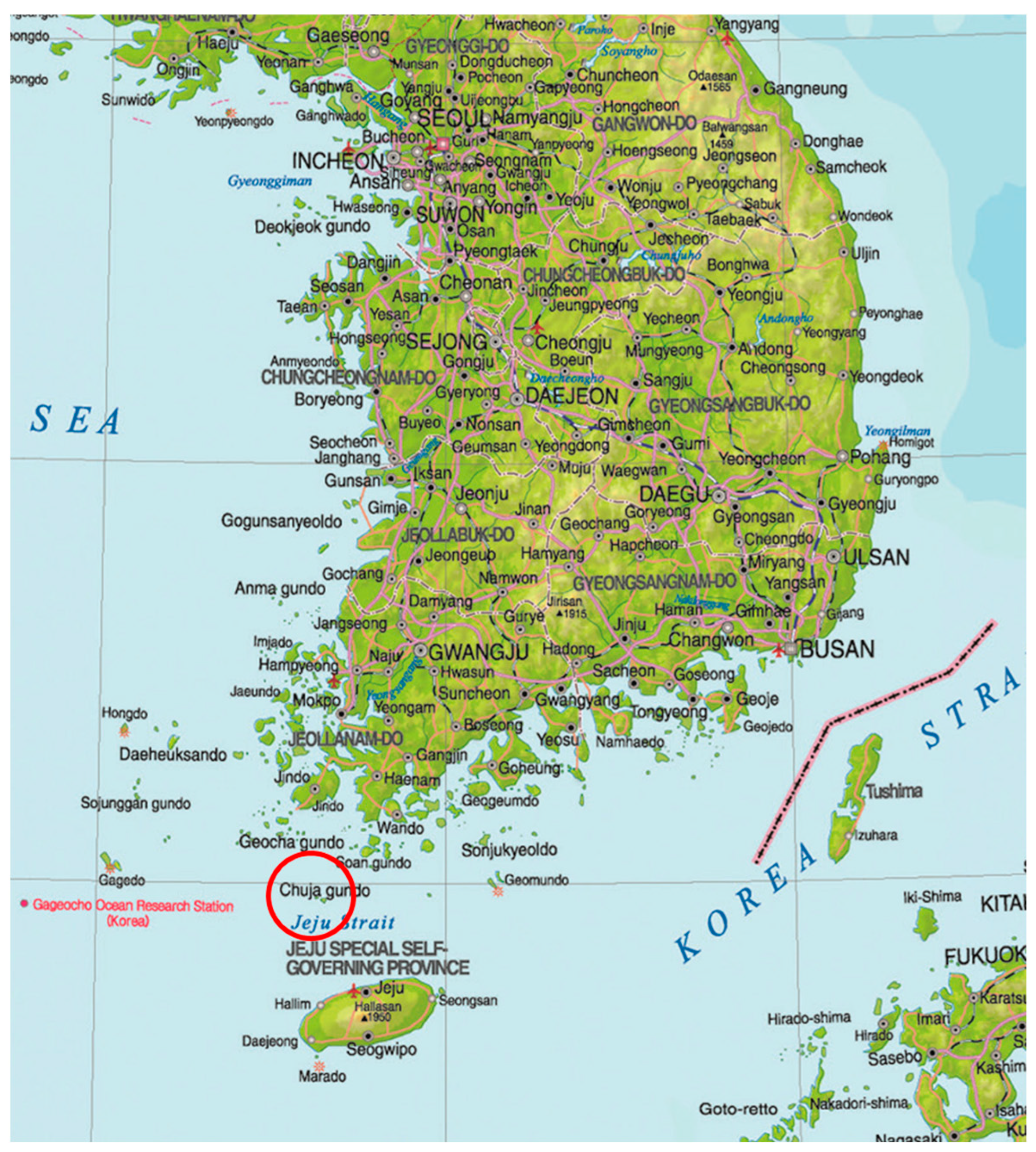
In this section, marine environmental and wave characteristics were analyzed using observation data from the Chujado marine buoy near Jeju. Significant wave height, period, wave direction, and ship-relative headings were statistically examined to identify representative operating conditions. Furthermore, extreme value analysis based on the GEV distribution was performed to estimate design wave conditions.

2.2.1. Marine Meteorological Data

Marine meteorological and wave data were obtained from the Korea Meteorological Administration (KMA) through its open data portal. Measurements were taken by the Chujado marine buoy (Station No. 22184), which has continuously collected sea-state parameters for over ten years, starting from 2014. The buoy records sea-surface motion via accelerometers and provides derived quantities such as significant wave height (Hs) and mean wave period (Tz). The nearest buoy to the measured ferry routes was Chujado, located approximately 49 km northwest of Jeju Port. Figure 2 shows its geographical pogsition, and

Table 2. Information on the Chujado marine Meteorological buoy.

Station Name (Standard Station Number)	Chujado (22184)
Managing Organization	Korea Meteorological Administration, Jeju Regional Meteorological Office, Observation Division
Address	Offshore, 49 km northwest of Jeju Port, Jeju-si, Jeju Special Self-Governing Province
Observation Start Date	Operational data
Observation Interval (minutes)	30
Coordinates (WGS84)	Latitude: 33.79361/Longitude: 126.14111111
Water Depth (m)	85

lists detailed specifications.

2.2.2. Wave Statistics

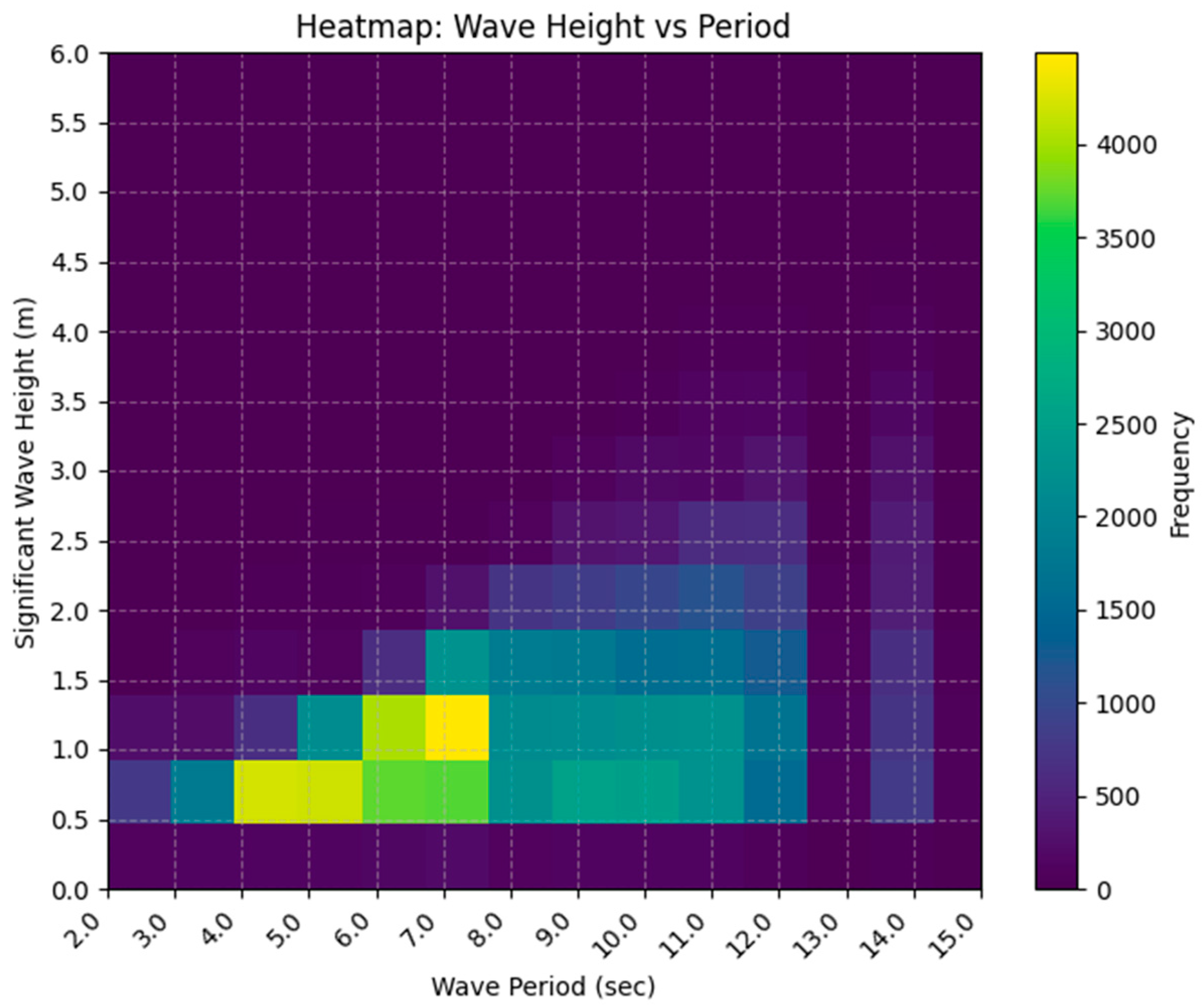
Based on a decade of observations from the Chujado buoy, the joint distribution of significant wave height (Hs) and mean zero-crossing period (Tz) was analyzed.

• The mean and median of Hs were 1.06 m and 0.9 m, respectively, indicating predominance of low waves.
• The most frequent range was 0.5–1.0 m (36%), followed by 1.0–1.5 m (21%) and 0.0–0.5 m (24%).
• Waves exceeding 2.0 m accounted for only ~9%, and extreme waves above 5.0 m were rare (0.04%), with the maximum recorded Hs = 6.4 m.
• The mean and median Tz were 5.2 s and 4.9 s, with the dominant range of 3–5 s (43%), followed by 5–7 s (32%) and 7–9 s (14%).
• Long-period waves exceeding 9 s were scarce (≈3%), with a maximum Tz = 28.6 s.

These characteristics represent a typical coastal and island-sea wave climate, serving as baseline data for port design, offshore-structure stability assessment, and ship-operational safety analysis. The joint distribution pattern between Hs and Tz, illustrating the dominance of low-height and short-period waves, is visualized in Figure 3, which presents a heatmap of wave period versus significant wave height at Chujado, Jeju. The figure clearly demonstrates the concentration of wave energy in the low-Hs and moderate-Tz region, confirming the mild sea-state characteristics of the observation area.

2.2.3. Wave Direction Distribution

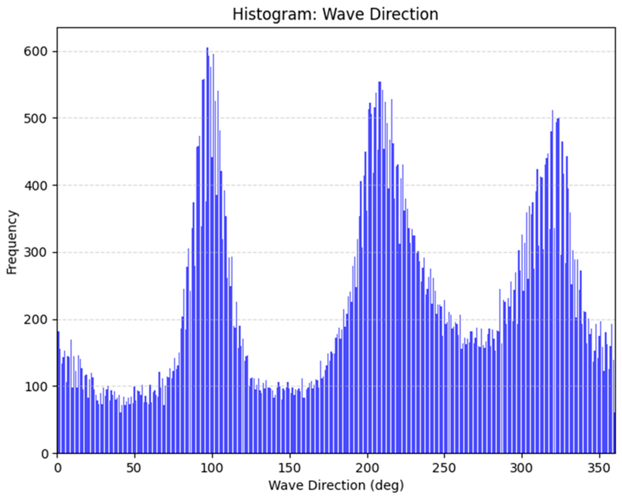
A directional histogram was used to visualize the occurrence frequency of waves by heading. The analysis revealed dominant propagation directions around south–southeast and northeast, reflecting local meteorological and topographical influences such as monsoonal winds and the island’s coastal geometry.

As shown in Figure 4, the histogram exhibits three distinct directional peaks, indicating that waves most frequently originated from approximately 100°, 215°, and 330°. These peaks correspond to the E–SE, S–SW, and NW sectors, respectively, suggesting the presence of multiple prevailing wave systems affecting the Chujado region throughout the year. This directional clustering pattern highlights the anisotropy of the local sea state and aligns with the regional wind and swell propagation characteristics observed in the East China Sea and adjacent coastal waters.

2.2.4. Ship Heading Analysis Based on GPS

To identify representative relative wave headings for motion analysis, the heading angles from GPS tracks were statistically analyzed. This supports selecting relevant wave-approach conditions for HydroD-based motion response simulations. In HydroD, the wave direction is defined clockwise from true north, identical to the ship’s heading angle. However, the dynamically important parameter is the relative wave heading ($\mathit{\beta }$)—the direction of wave incidence relative to the ship’s bow.

$$\mathit{\beta }={\mathit{\theta }}_{\mathit{w}\mathit{a}\mathit{v}\mathit{e}}-{\mathit{\theta }}_{\mathit{s}\mathit{h}\mathit{i}\mathit{p}}$$

(1)

where

• ${\mathit{\theta }}_{\mathit{w}\mathit{a}\mathit{v}\mathit{e}}$: absolute wave direction (° from true north),
• ${\mathit{\theta }}_{\mathit{s}\mathit{h}\mathit{i}\mathit{p}}$: ship heading angle (° from true north),
• $\mathit{\beta }$: relative wave heading (° from bow; port = −, starboard = +).

Statistical analysis identified two dominant ship headings:

• Heading 1: 189° (southwest),
• Heading 2: 25° (north–northeast).

Using absolute wave directions of 97° and 320°, the resulting relative headings are summarized in

Table 3. Relative wave heading angle calculation.

Case	Heading (°)	Wave Direction (°)	Relative Wave Direction $({\mathit{\theta }}_{\mathit{r}\mathit{e}\mathit{l}}$)	Type
A	189	97	−92°	Beam Sea (Port)
B	189	320	131°	Quartering Sea (Starboard)
C	25	97	72°	Quartering Sea (Starboard)
D	25	320	−65°	Quartering Sea (Port)

.

From the viewpoint of ship response characteristics:

• Beam Sea (±90°): largest roll amplitude,
• Quartering Sea (±45–135°): coupled roll–yaw motion → broaching risk,
• Head Sea (0°): dominant pitch/heave response,
• Following Sea (180°): degraded course stability.

Cases A (−92°) and D (−65°), therefore, correspond to port-beam and port-quartering seas, which are expected to produce the largest roll responses and lowest directional stability.

However, analysis based solely on observed headings cannot fully represent the range of wave-encounter scenarios required for design studies. To encompass broader directional sensitivity—including hydrodynamic symmetry and wave-directional effects—eight headings were analyzed at 45° intervals from 0° to 315°, enabling a comprehensive directional response map and identification of worst-case conditions.

2.2.5. Extreme Wave Generation Using GEV Distribution

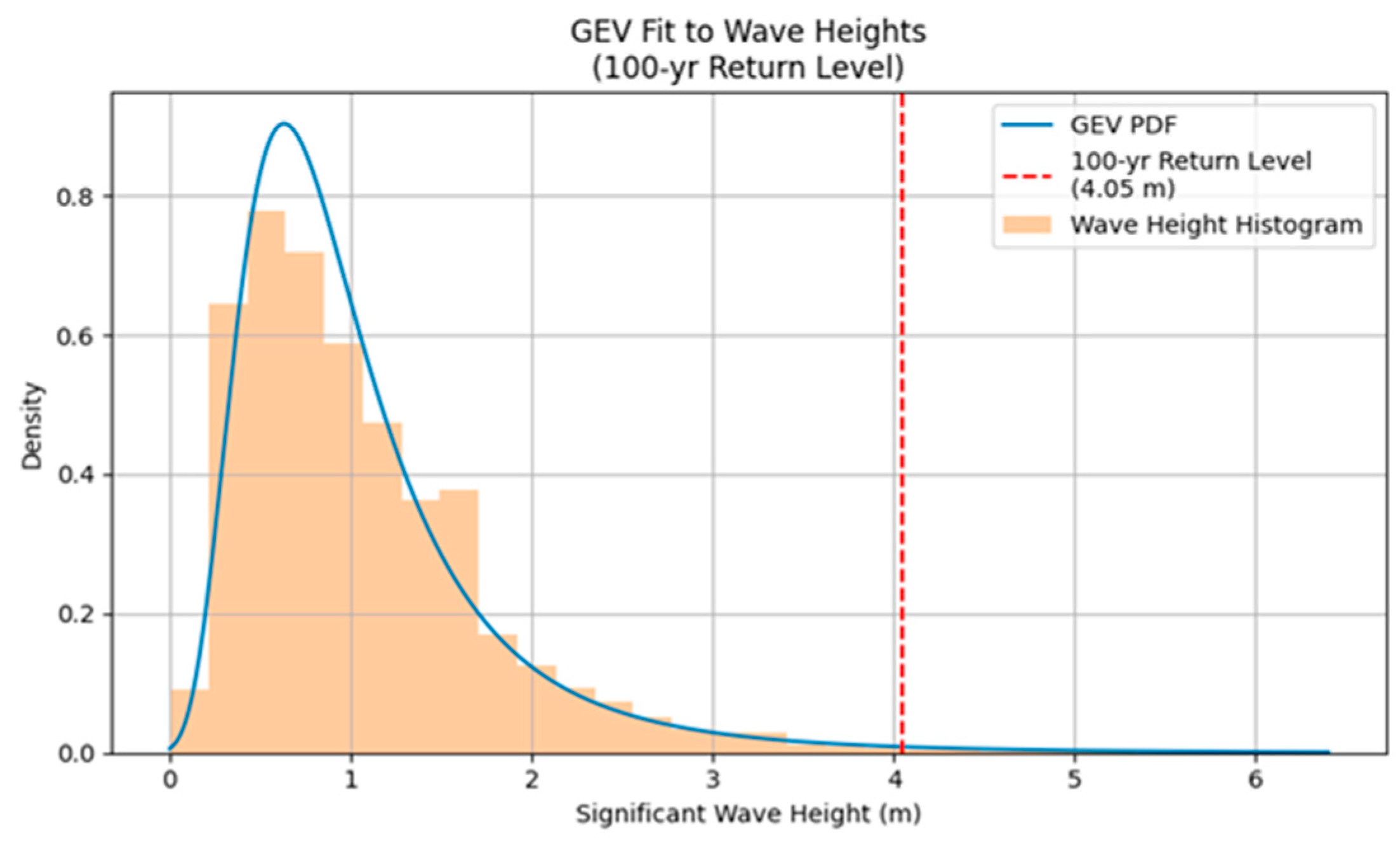
Extreme value analysis (EVA) was performed to estimate return-level wave conditions corresponding to 50-, 100-, and 200-year return periods. The generalized extreme value (GEV) distribution was fitted to the long-term Hs dataset:

$$\mathit{F}(\mathit{x})=\mathbf{e}\mathbf{x}\mathbf{p}[-{\left(\mathbf{1}+\mathit{\xi }{\displaystyle \frac{\mathit{x}-\mathit{\mu }}{\mathit{\sigma }}}\right)}^{-\mathbf{1}/\mathit{\xi }}]$$

(2)

where

• $\mathit{x}$: random variable (significant wave height),
• $\mathit{\mu }$: location parameter (central tendency),
• $\mathit{\sigma }$: scale parameter (distribution width),
• $\mathit{\xi }$: shape parameter (tail heaviness).

This formulation yields design extreme wave heights, with the mean wave period corresponding to each return level used as the associated period. Figure 5 presents the GEV fitting, and

Table 4. Wave condition extracted using the GEV distribution.

Wave Condition	GEV Distribution	Significant Wave Height	Wave Period	Wave Direction
Wave 1	10 years	2 m	7.5 s	0–315° (45° interval)
Wave 2	100 years	4 m	8.5 s
Wave 3	200 years	4.9 m	9.5 s
Wave 4	500 years	6.3 m	9.5 s

lists the resulting design conditions.

2.3. DNV Sesam Package and HydroD

Sesam is an integrated suite of software tools designed for hydrodynamic and structural analysis of ships and offshore structures. The system is based on the displacement formulation of the Finite Element Method (FEM) and offers specialized capabilities through its major modules, including GeniE, HydroD, Sima, and Sesam Wind Manager, each tailored to the analysis requirements of marine and offshore industries [19].

Among these tools, HydroD serves as the core software for performing stability and hydrodynamic analyses of ships and offshore platforms within the Sesam package. A key feature of HydroD is its integrated analysis framework, which allows users to perform hydrostatic (static) analysis, frequency-domain analysis, and time-domain analysis based on a common model. This integrated workflow supports comprehensive evaluations such as structural performance assessment, stability verification, long- and short-term statistical analysis, and design-wave studies [19,20].

Frequency-domain hydrodynamic responses are computed using the Wadam module, whereas time-domain simulations are executed through the Wasim module. HydroD also incorporates nonlinear analysis capabilities, enabling more accurate representation of complex motion behaviors that occur under realistic ocean environmental conditions.

2.4. Numerical Simulation (HydroD-Wasim)

HydroD, a core module within DNV’s Sesam software suite, performs hydrostatic and hydrodynamic analyses for ships and offshore structures. Its integrated workflow enables: hydrostatics (stability), frequency-domain analysis, and time-domain simulations (Wasim module), all using a unified geometric model. These analyses support stability evaluation, long- and short-term statistics, and design-wave assessments. Time-domain results can directly feed into structural fatigue or ultimate-load evaluations. HydroD also supports nonlinear time-domain analysis, allowing realistic modeling of complex sea-state responses.

Three-dimensional geometric models of Car Ferry A and B were generated. Hydrodynamic force computation requires a panel model whose surface mesh matches the actual hull form defined by the PLN model. The PLN model typically represents the port-side half of the hull, which HydroD mirrors about the centerline to construct the full panel model. Figure 6 and Figure 7 show PLN and corresponding panel models for both vessels.

Simulation Configuration

A total of 384 simulation cases were designed to reflect diverse operating and damage scenarios. Key input parameters included ship speed, hull condition, and external sea states (Hs, Tz, wave direction).

• Ship speed: 21 kn (service), 10 kn (reduced), and 0 kn (stationary).
• Hull condition: Intact, and three flooding scenarios (bow, midship, stern).
• Wave environment: Significant wave heights 2.0, 4.0, 4.9, 6.3 m; mean periods 7.5, 8.5, 9.5 s; eight directions at 45° intervals (0–315°).

These combinations yield (

Table 5. Analysis scenario input parameters.

Parameter	Values
Ship speed (m/s)	10.65/5/0
Hull condition	Intact/Bow flooding/Midship flooding/Aft flooding
Hs (m)	2/4/4.9/6.3
Tz (s)	7.5/8.5/9.5/9.5
Wave direction (°)	0/45/90/135/180/225/270/315
Total cases	384

)

$$3\left(speed\right)\times 4\left(condition\right)\times 4\left(Hs\right)\times 3\left(Tz\right)\times 8\left(direction\right)=384 cases$$

The configuration encompasses a wide range of realistic operational states, from calm to extreme seas and from intact to damaged hulls, forming a comprehensive dataset for both stability assessment and motion-prediction modeling. Figure 8 shows the HydroD–Wasim time-domain motion-analysis results for Car Ferry A, illustrating the vessel’s dynamic responses, such as roll and pitch.

3. Methodology

3.1. Data Preprocessing

The first step in developing the ship-motion prediction algorithm was to construct a numerical dataset using HydroD-Wasim-based time-domain simulations.

A total of 384 motion-simulation cases were generated by combining all analysis parameters described in Section 2. After removing erroneous data, the remaining datasets were used for model training.

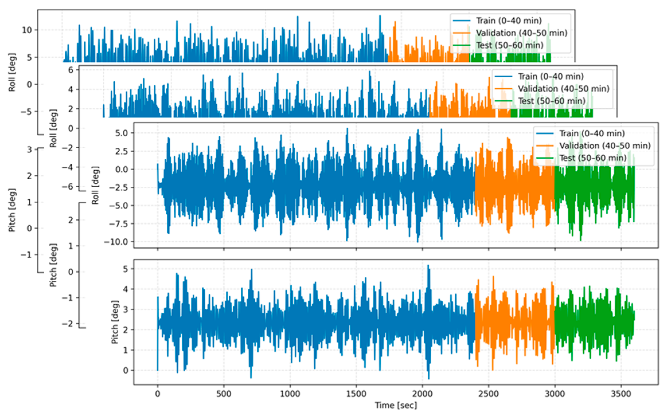
Each simulation produced a 10 Hz time-series record for 3600 s (1 h) of motion responses. To simulate real-world forecasting conditions, each sequence was divided into three disjoint temporal segments:

• Training data: 0–2400 s (first 40 min);
• Validation data: 2400–3000 s (next 10 min);
• Test data: 3000–3600 s (last 10 min).

This non-overlapping split ensures that the model learns generalizable temporal patterns rather than memorizing short-term histories.

Validation sets were used for hyperparameter tuning and model selection, while test sets were reserved for final generalization evaluation.

Figure 9 illustrates the segmentation scheme of the dataset.

3.2. Deep-Learning Models

3.2.1. LSTM Model

The Long Short-Term Memory (LSTM) network extends the conventional recurrent neural network (RNN) architecture to overcome the vanishing gradient problem, a phenomenon in which gradients diminish exponentially during backpropagation through time, making it difficult for standard RNNs to learn long-range dependencies. LSTM mitigates this issue by introducing a memory cell and gated mechanisms that preserve and regulate gradient flow over extended sequences. Its core components include the cell state and three gates—forget, input, and output—which dynamically control the flow of information through the sequence [21,22].

• Forget gate: Decides which past information to discard.

  $$f_t=\sigma (W_f\cdot \left[h_{t-1}, x_t\right]+b_f$$

  (3)
• Input gate: Determines what new information to store in the cell.

  $$i_t=\sigma (W_i\cdot \left[h_{t-1},x_t\right]+b_i$$

  (4)

  $$\widetilde{C_t}=\mathrm{t}\mathrm{a}\mathrm{n}\mathrm{h}(W_C\cdot \left[h_{t-1},x_t\right]+b_C)$$

  (5)
• Cell state update: Integrates retained and new information.

  $$C_t=f_t\odot C_{t-1}+i_t\odot \widetilde{C_t}$$

  (6)
• Output gate: Controls which part of the cell state is propagated.

  $$O_t=\sigma (W_O\cdot [h_{t-1},x_t ]+b_O)$$

  (7)

  $$h_t=O_t\odot tanh\left(C_t\right)$$

  (8)

Let $\mathsf{\sigma }$ denote the sigmoid function, and let ⊙ represent the element-wise (Hadamard) product. The LSTM’s gated structure facilitates stable gradient propagation and enables robust learning over long sequences, offering significantly improved performance compared with standard RNNs. The detailed configuration of the LSTM model used in this study is summarized in

Table 6. LSTM model configuration.

Category	Specification
Input/Output	Input: ($B, T_{in}, inpu{t}_{dim}$); Output: ($B, T_{out}$)
Model structure	LSTM ($inpu{t}_{dim}$→ hidden = 128, $nu{m}_{layers}$= 2, Dropout = 0.1, batch first = True)
Pooling	Mean pooling of all LSTM time outputs → ($B$, 128)
Prediction head	Dropout (0.1) → Linear (128 → $T_{out}$× 2) → output ($\mathrm{m}\mathrm{e}\mathrm{a}\mathrm{n} \mu + \mathrm{l}\mathrm{o}\mathrm{g}-\mathrm{v}\mathrm{a}\mathrm{r}\mathrm{i}\mathrm{a}\mathrm{n}\mathrm{c}\mathrm{e} log{\sigma }^2$)
Loss function	Composite: MSE + β·(1 − PICP) + γ·PINAW,
Uncertainty estimation	Same as Transformer ($\mu , log{\sigma }^2 \to \sigma$, compute ±1.96σ interval)
Optimizer	AdamW (lr = 3 × 10−4, wd = 1 × 10−2) with linear warm-up (10%) and CosineAnnealingLR
Epochs/Batch size	80 epochs/batch size = 128

Notes: the arrow symbol “→” indicates a mapping or transformation in the model architecture. In linear layers, it denotes the change of dimensionality (e.g., Linear (256 → 128) means input dimension 256 is projected to 128). In sequences of operations, it represents the ordered flow from one operation to the next.

.

3.2.2. Transformer Model

The Transformer architecture, originally introduced by Vaswani et al. in “Attention Is All You Need,” removes the sequential dependency inherent in RNN-based models by employing a self-attention mechanism, thereby enabling full parallelization and efficient learning of long-range temporal relationships [23,24,25]. It has since become the foundation of numerous state-of-the-art deep-learning models.

Key characteristics:

• Self-Attention: Captures contextual relationships among all positions in the input sequence.
• Parallel computation: Processes all input tokens simultaneously.
• Long-range dependency handling: Models global dependencies without loss of temporal coherence.

A central reason the Transformer supports parallel computation is that the self-attention mechanism does not require sequential recursion. Unlike RNNs, which compute hidden states one time step at a time (i.e., $h_t$ depends on $h_{t-1}$), the Transformer forms query ($Q$), key ($K$), and value ($V$) matrices for the entire sequence in a single operation. Because attention weights for every pair of positions are computed through matrix multiplications, the dependencies among all tokens are evaluated simultaneously. These operations—projection to Q/K/V, scaled dot-product attention, softmax, and linear output projection—are implemented as batched matrix operations, which are inherently parallelizable on modern hardware such as GPUs.

The scaled dot-product self-attention is defined as:

$$Attention(Q,K,V)=softmax\left({\displaystyle \frac{Q{K}^T}{\sqrt{d_k}}}\right)V$$

(9)

where $Q,K,V$ are the query, key, and value matrices, and $d_k$ is the dimension scaling factor.

Multi-head attention allows the model to jointly attend to information from different representation subspaces:

$$MultiHead(Q,K,V)=Concat\left(head1,\dots ,headh\right)W^O$$

(10)

Additional architectural components include positional encoding (either sinusoidal or learned) to inject temporal order, feed-forward networks (FFNs) that apply nonlinear transformations to enhance expressive capacity, and residual connections with layer normalization to stabilize training and mitigate gradient degradation. The detailed configuration of the Transformer model employed in this study is summarized in

Table 7. Transformer model configuration.

Category	Specification
Input/Output	Input: ($B, T_{in}, inpu{t}_{dim}$); Output: ($B, T_{out}$)
Preprocessing	Linear ($inpu{t}_{dim}$→ 128); learned positional encoding initialized with N (0, 0.022)
Encoder	TransformerEncoder × 3 ($d_{model}$= 128, nhead = 8, $di{m}_{ff}$= 512, Dropout = 0.1, activation = GELU, batch_first = True) + final LayerNorm
Concatenation	Concatenate last hidden state ($h_{last})$ and mean-pooled feature $(h_{mean}$) → ($B$, 256)
Prediction head	Linear (256 → 128) → GELU → Dropout (0.1) → Linear (128 → $T_{out}$× 2) ($\mu + log{\sigma }^2$)
Loss function	Composite: MSE (μ, y) + β·(1−PICP) + γ·PINAW
Uncertainty estimation	Decompose output into μ and σ = exp (0.5·logσ2); derive 95% CI = μ ± 1.96σ
Optimizer	AdamW (lr = 3 × 10−4, weight_decay = 1 × 10−2)
Scheduler	Linear warm-up (10% epochs) → CosineAnnealingLR
Epochs/Batch size	80 epochs/batch size = 128

Notes: the arrow symbol “→” indicates a mapping or transformation in the model architecture. In linear layers, it denotes the change of dimensionality (e.g., Linear (256 → 128) means input dimension 256 is projected to 128). In sequences of operations, it represents the ordered flow from one operation to the next.

.

3.3. Uncertainty Quantification

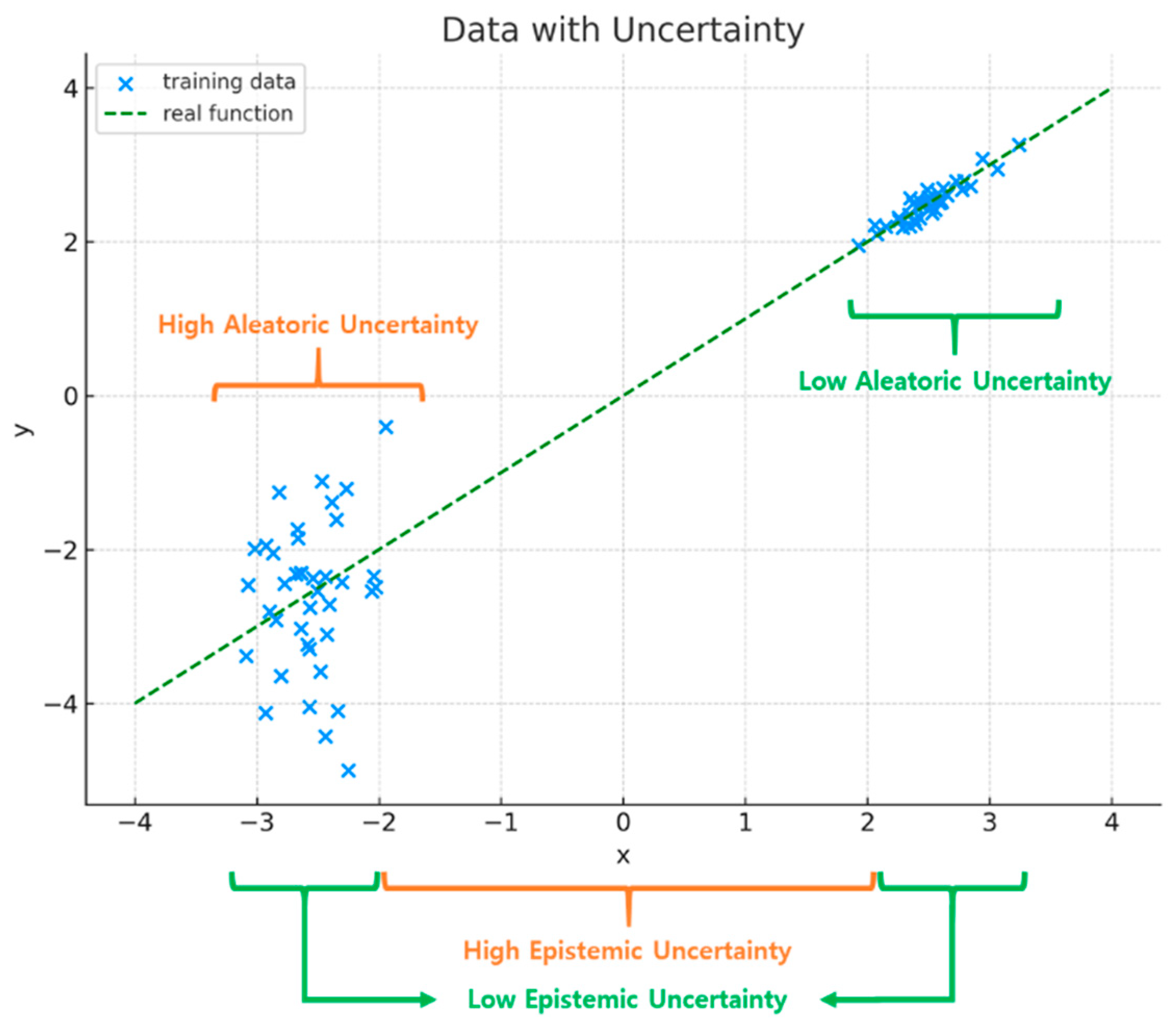
Uncertainty reflects the degree of information insufficiency in describing how well model predictions represent actual physical phenomena. In machine learning and deep learning, uncertainty is generally classified into two major categories: aleatoric and epistemic.

• Aleatoric Uncertainty (Data Uncertainty):

Originates from the inherent randomness of the data itself—sensor noise, environmental variability (e.g., sea-state fluctuations in wave height, period, or wind), and other irreducible sources.

2.

Epistemic Uncertainty (Model Uncertainty):

Arises from the model’s limited knowledge due to insufficient training data, poor coverage of input conditions, or structural limitations. Unlike aleatoric uncertainty, epistemic uncertainty can theoretically be reduced through additional data or improved modeling.

Der Kiureghian and Ditlevsen [26] emphasized that conflating aleatory and epistemic components can distort risk assessment in engineering systems. Later, Kendall and Gal [27] extended this framework to deep learning, demonstrating that explicitly modeling both uncertainty types in Bayesian neural networks significantly enhances predictive reliability.

In the context of ship-motion forecasting, simply predicting future values of roll or pitch is insufficient. It is equally crucial to quantify how confident the model is in its predictions—particularly under out-of-distribution conditions, such as extreme sea states or damaged-hull scenarios. Without uncertainty quantification, models risk overconfidence, yielding deceptively precise yet unreliable forecasts. Incorporating uncertainty analysis, therefore, establishes the foundation for trustworthy model deployment, enabling risk-aware control systems, onboard decision support, and safer ship operations under uncertain conditions.

Figure 10 illustrates the conceptual distinction between these two uncertainty types. Aleatoric uncertainty represents the intrinsic variability within the observed data, while epistemic uncertainty denotes the model’s lack of confidence stemming from incomplete knowledge. The diagram clarifies that both sources of uncertainty jointly influence prediction reliability, yet differ in their reducibility and interpretation.

3.3.1. Monte Carlo Dropout

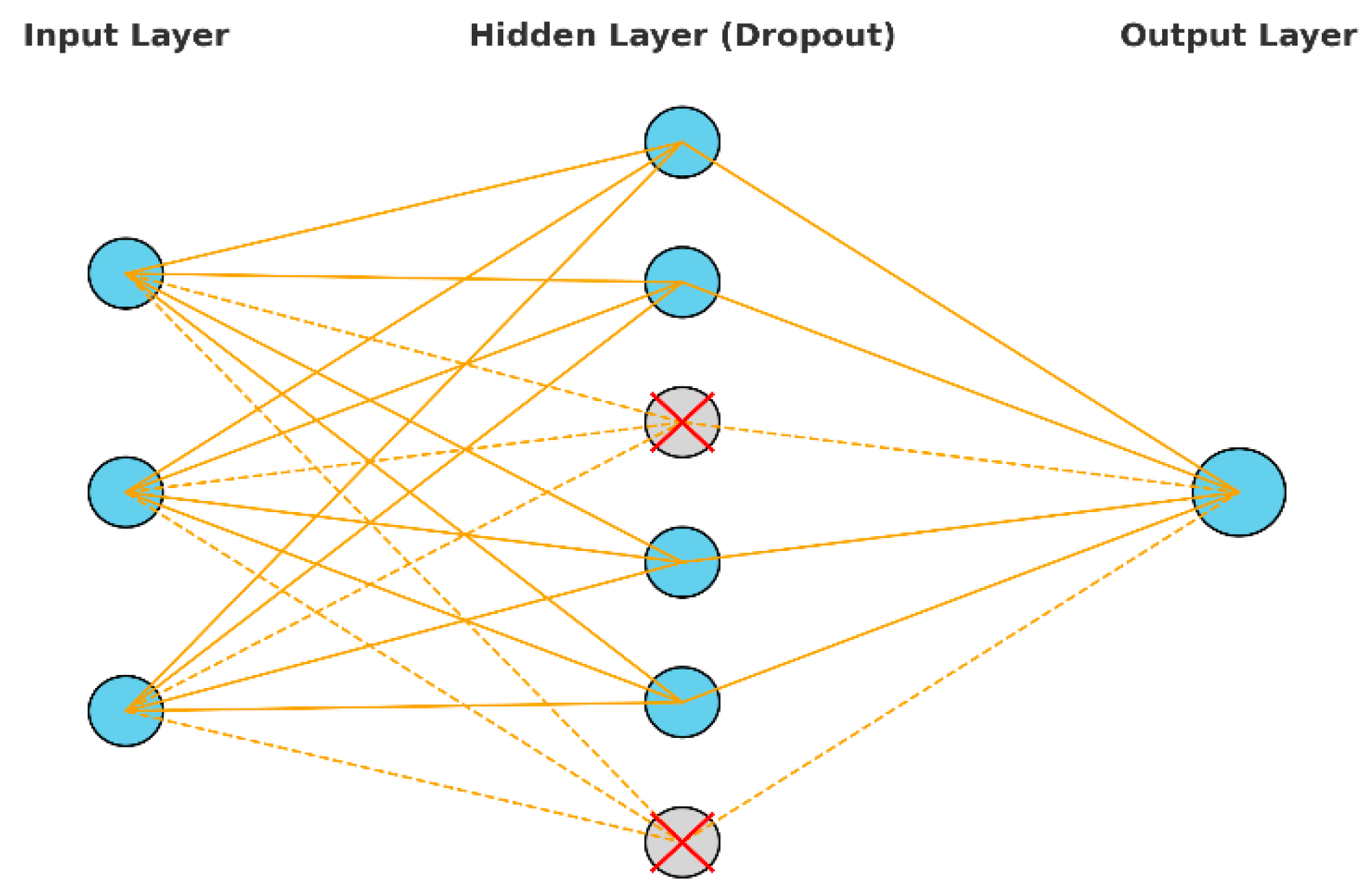
The Monte Carlo Dropout (MC Dropout) technique, introduced by Gal & Ghahramani [28], provides a simple yet effective Bayesian approximation for quantifying predictive uncertainty in deep neural networks.

Traditionally, Dropout randomly deactivates neurons during training to prevent overfitting. Gal and Ghahramani demonstrated that retaining Dropout at inference enables the model to generate a set of stochastic outputs, approximating a Bayesian posterior distribution over the network weights.

Let $K$ denote the number of stochastic forward passes (Dropout samples) and ${\widehat{y}}^t$ the prediction at the $t^{th}$ trial. The predictive mean and variance are computed as:

$$\overline{y}={\displaystyle \frac{1}{K}}\sum _{t=1}^K{\widehat{y}}_t, Var(y)={\displaystyle \frac{1}{K}}\sum _{t=1}^K{\left({\widehat{y}}_t-\overline{y}\right)}^2$$

(11)

Here, the variance represents epistemic uncertainty estimated from model variability. Mathematically, MC Dropout can be interpreted as an approximation to a Deep Gaussian Process, effectively enabling Bayesian inference via simple stochastic forward passes—without retraining or architectural modification.

Advantages:

• Implementation simplicity: Any Dropout-enabled network can estimate uncertainty by enabling Dropout at inference.
• No additional training: Requires only repeated stochastic forward passes.

Figure 11 illustrates the underlying principle of MC Dropout. Repeated stochastic inferences for the same input generate a predictive distribution rather than a single deterministic output, from which both the mean prediction and the confidence interval can be derived. This approach enables visual and quantitative interpretation of the model’s uncertainty—wider intervals indicating higher epistemic uncertainty under unfamiliar or extreme input conditions. In this study, the number of MC dropouts was set to 30.

In this study, MC Dropout was applied to both the Transformer-based model and the LSTM-based model to consistently quantify epistemic uncertainty across different neural network architectures.

For the Transformer model, Dropout was incorporated into all hidden units of the fully connected layers in the output regression head, as well as after each self-attention and feed-forward sublayer. A Dropout rate of 0.1 was used, with neurons randomly deactivated following a Bernoulli distribution.

For the LSTM model, MC Dropout was implemented by applying Dropout to the recurrent network’s hidden layers and the subsequent fully connected regression layer. Specifically, the Dropout mechanism was activated between LSTM layers and on the output layer, while maintaining deterministic recurrence within each LSTM cell (i.e., no Dropout on recurrent connections to preserve temporal memory). This design allows the LSTM model to produce stochastic outputs at inference while retaining stable sequential representations.

In both architectures, the same MC Dropout procedure was used at inference: Dropout remained activated, and 30 stochastic forward passes were conducted to estimate the predictive mean and epistemic uncertainty through output variance. This unified strategy enables a fair comparison of uncertainty characteristics between sequence models with fundamentally different structural properties.

3.3.2. Loss Function

To enhance both the prediction accuracy and the reliability of uncertainty quantification, a composite loss function was designed as follows:

$${\mathcal{L}}_{total}=\alpha ·MSE + \beta ·\left(1-PICP\right)+ \gamma ·PINAW$$

(12)

where $\alpha =1, \beta =2, and \gamma =0.1$ are the weighting coefficients that balance the contributions of accuracy, coverage, and interval width, respectively. The MSE component improves the accuracy of point predictions, while the (1 − PICP) and PINAW terms regulate the reliability and compactness of the predictive intervals.

The weighting coefficients were selected based on the following considerations. First, coverage reliability (PICP) is the primary requirement in uncertainty quantification; insufficient coverage severely undermines the practical usefulness of prediction intervals. Therefore, the coefficient $\beta$ was set larger than $\alpha$ to penalize coverage deficiency more strongly. Second, excessively wide intervals degrade interpretability even when coverage is satisfied. Thus, the PINAW term was assigned a smaller weight ($\mathsf{\gamma }$) to encourage compact intervals while preventing over-penalization that could compromise PICP. Finally, preliminary sensitivity tests confirmed that the ratio $\mathsf{\alpha }:\mathsf{\beta }:\mathsf{\gamma }=1:2:0.1$ provides a stable trade-off—improving coverage without inflating interval width and maintaining competitive point-prediction accuracy.

Consequently, this formulation yields a balanced compromise between point prediction accuracy and uncertainty quantification quality, which is essential for robust ship motion forecasting under uncertain environmental conditions.

(1)

Mean Squared Error (MSE)

$$MSE={\displaystyle \frac{1}{N}}\Sigma {(y_i-{ŷ}_i)}^2$$

(13)

The mean squared error evaluates the average squared difference between the observed value $y_i$ and the predicted mean ${ŷ}_i$. It primarily measures the point estimation accuracy, penalizing larger deviations more heavily. Minimizing MSE encourages the model to produce accurate deterministic predictions.

(2)

Prediction Interval Coverage Probability (PICP)

$$PICP={\displaystyle \frac{1}{N}}\Sigma I(y_i\in [{ŷ}_i^L, {ŷ}_i^U\left]\right)$$

(14)

The PICP represents the coverage rate of the prediction intervals, defined as the proportion of actual observations that fall within the predicted lower and upper bounds $[{ŷ}_i^L, { ŷ}_i^U]$. A higher PICP indicates greater reliability of the predicted intervals. In the loss function, the term (1 − PICP) is used so that increasing PICP (i.e., better coverage) reduces the total loss.

(3)

Prediction Interval Normalized Average Width (PINAW)

$$PINAW={\displaystyle \frac{1}{NR}} \Sigma \left({ŷ}_i^U-{ŷ}_i^L\right), where R=\mathit{max}\left(y\right)-\mathit{min}\left(y\right)$$

(15)

PINAW quantifies the normalized width of the prediction intervals. A smaller PINAW implies narrower intervals, reflecting greater precision in uncertainty estimation. However, excessively narrow intervals may lead to low PICP, so this metric is used in conjunction with the PICP term to maintain a balance between reliability and sharpness.

4. Results and Discussion

This section presents the prediction results obtained from the motion-analysis datasets and evaluates the performance of the Transformer and LSTM models using three quantitative metrics:

• MSE—prediction accuracy,
• PICP—reliability of the confidence interval,
• PINAW—width of the uncertainty interval.

Model behavior is analyzed with respect to key hydrodynamic parameters: significant wave height ($H_s$), wave period ($T_z$), wave direction, ship speed ($U$), and loading/damage condition ($L/C$).

4.1. Car Ferry A—Effect of Wave Height and Period

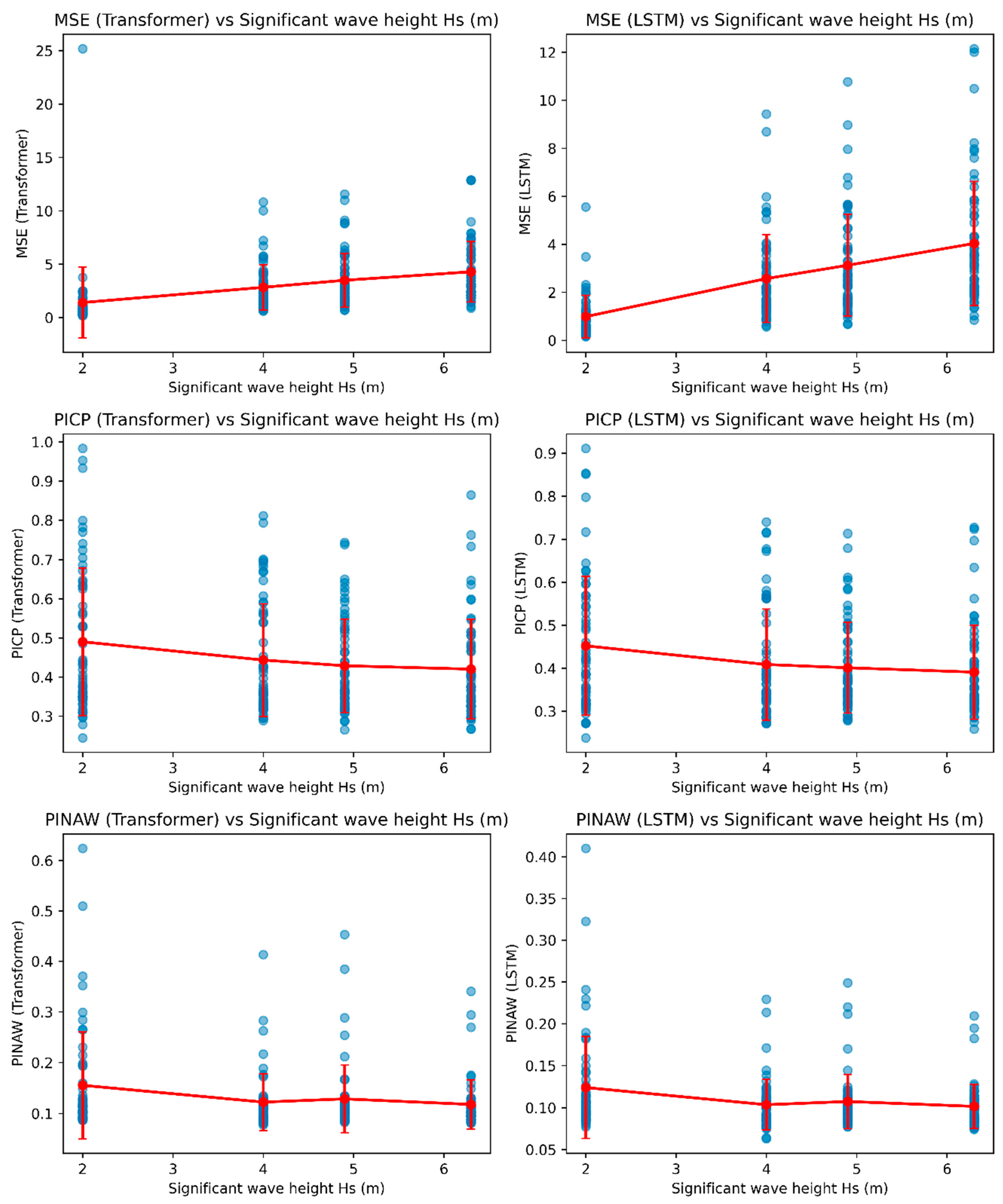
For Car Ferry A, both models exhibited an increase in MSE with rising wave height. As Hs increased from 2.0 m to 6.3 m, the Transformer consistently produced higher MSE than the LSTM, with an average difference of approximately 0.18. PICP values for both models were similar, although the Transformer’s mean PICP was marginally higher (+0.003), suggesting slightly broader confidence coverage. PINAW values were also higher for the Transformer (average +0.016), implying wider prediction intervals and a more conservative uncertainty estimation.

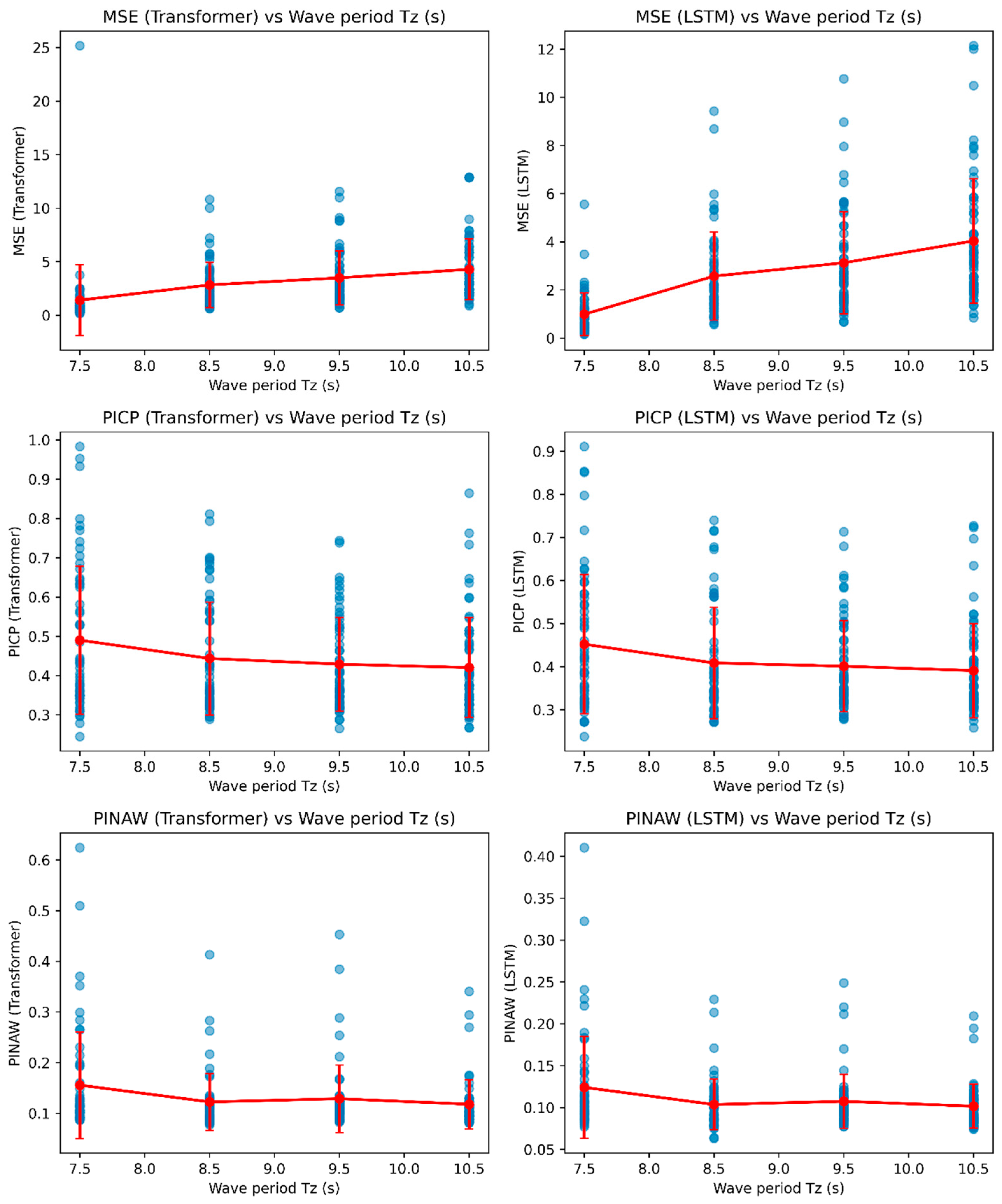
The analysis with respect to the wave period Tz showed comparable trends: MSE increased with longer periods (7.5 → 9.5 s), and the Transformer maintained a higher average MSE (+0.18). Overall, the LSTM achieved superior predictive accuracy, while the Transformer demonstrated broader but more conservative uncertainty bounds.

Figure 12 visualizes the variation in prediction performance metrics—MSE, PICP, and PINAW—with respect to significant wave height (Hs). Figure 13 presents the same performance metrics as a function of mean wave period (Tz), illustrating that prediction errors increase with longer wave periods.

4.2. Car Ferry A—Effect of Wave Direction

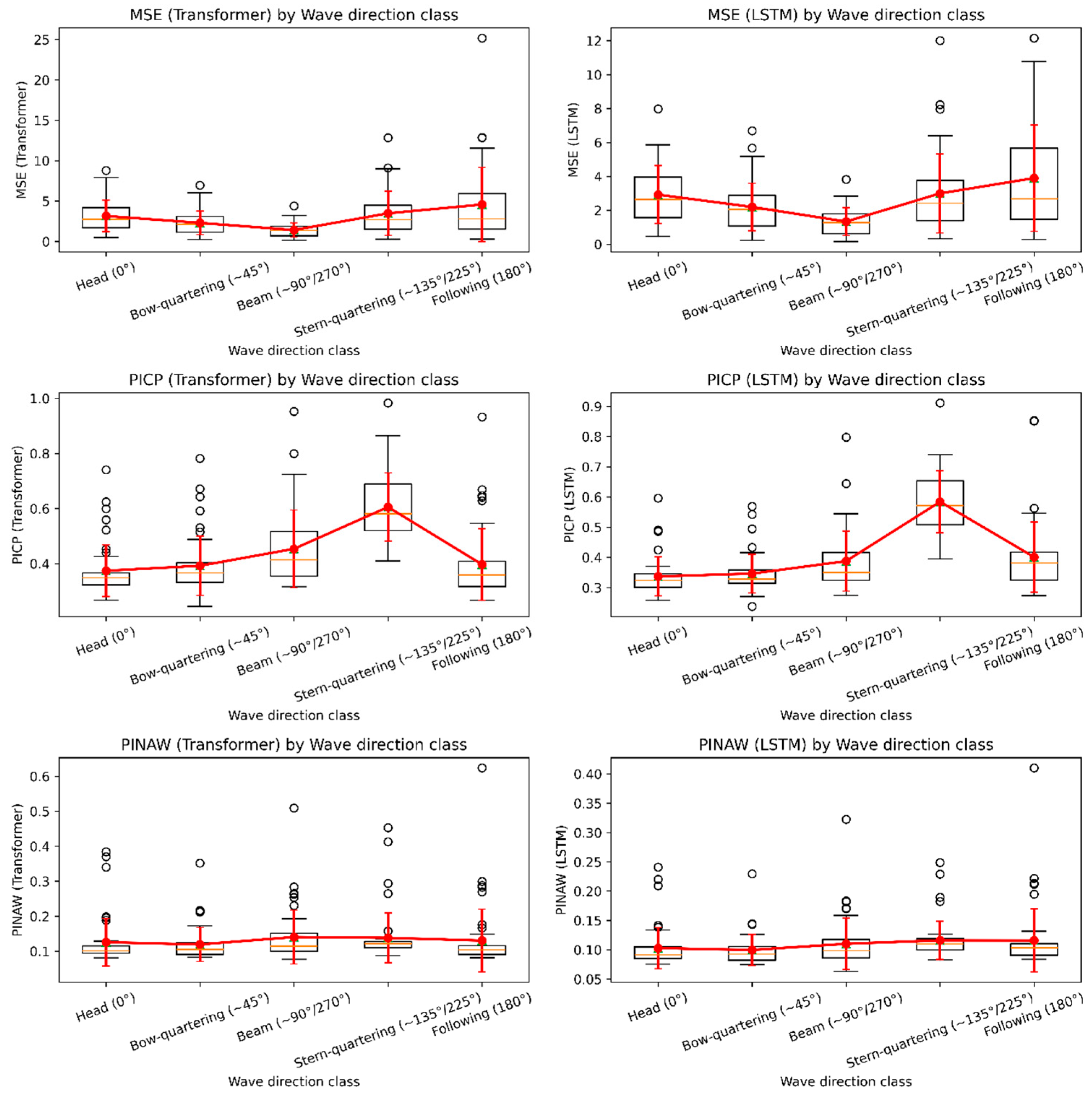
The predictive performance of the Transformer and LSTM models was compared with respect to wave direction (Figure 14).

Across all eight directional conditions, the Transformer consistently exhibited higher mean squared error (MSE) values than the LSTM. On average, the Transformer’s MSE was approximately 0.18 higher, indicating that the LSTM achieved greater predictive accuracy under varying directional conditions.

Although PICP values showed minor variations among directions, the Transformer recorded a slightly higher mean value of about +0.003, suggesting a marginally broader confidence coverage. In contrast, PINAW values were consistently larger for the Transformer by an average of 0.016, implying wider prediction intervals and a more conservative estimation of uncertainty.

In summary, the Transformer demonstrated a tendency toward broader but safer uncertainty bounds, while the LSTM maintained narrower intervals and higher prediction accuracy across all wave directions. Both models exhibited consistent directional trends, with the Transformer showing a more conservative and the LSTM a more efficient predictive behavior.

4.3. Car Ferry A—Effect of Ship Speed

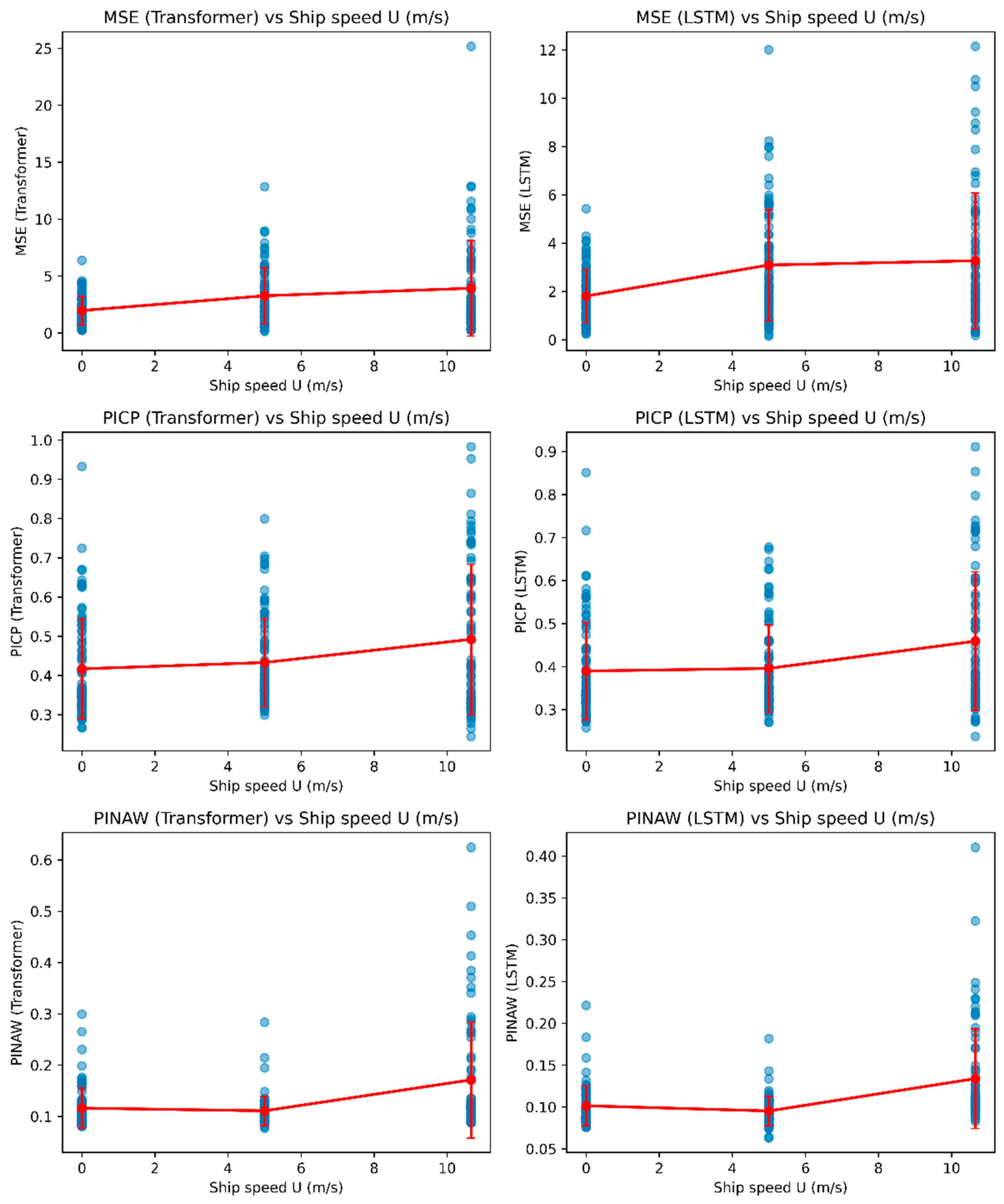
Both models showed decreasing MSE with increasing ship speed, indicating improved predictive stability at moderate and high speeds. LSTM consistently achieved lower MSE values by approximately 0.15–0.25, confirming its slightly better precision.

Meanwhile, PICP exhibited a mild decline as speed increased (−0.016 overall), with the Transformer maintaining a marginally higher average coverage (+0.003). PINAW widened progressively with speed, and the Transformer’s intervals were 0.015–0.02 broader than those of LSTM. Figure 15 illustrates these trends, showing the variation in prediction performance metrics (MSE, PICP, and PINAW) with ship speed (U).

4.4. Car Ferry A—Effect of Loading and Damage Condition

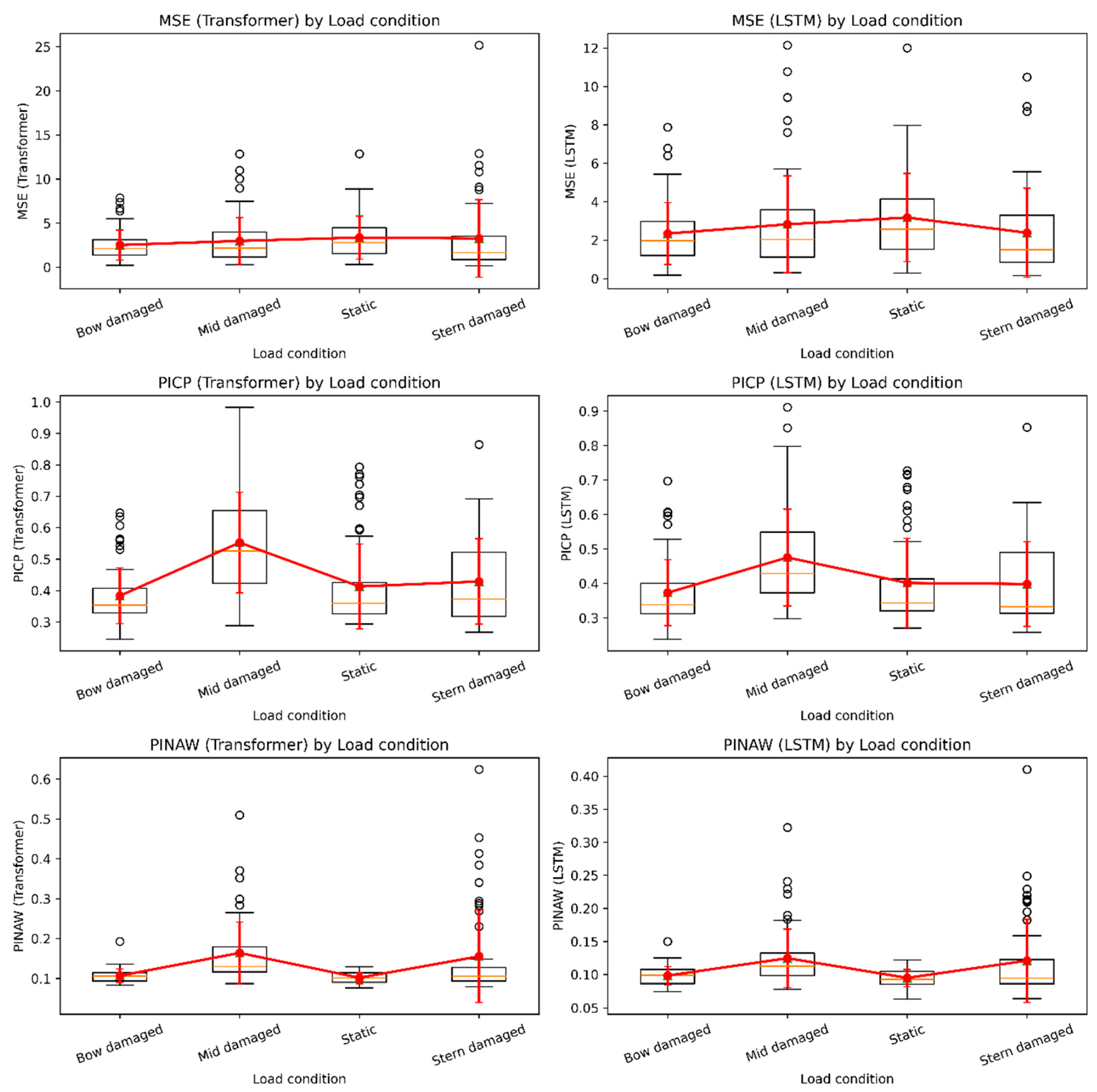
Across intact and flooded conditions (bow, midship, stern flooding), the LSTM model outperformed the Transformer in every scenario, with mean MSE differences around 0.18. The Transformer achieved slightly higher PICP (+0.005) and wider PINAW (+0.017). Thus, LSTM excels in predictive accuracy, while Transformer demonstrates superior robustness in uncertainty calibration (Figure 16).

4.5. Car Ferry B—Effect of Wave Height and Period

For Car Ferry B, a vessel with larger dimensions and lower transverse stability, both models showed increasing MSE with greater wave height. The Transformer’s mean MSE exceeded that of the LSTM by 0.32, reflecting amplified errors under nonlinear motion amplification. PICP values were 0.032 higher and PINAW 0.022 wider for the Transformer, confirming a conservative uncertainty evaluation. LSTM again achieved smaller prediction errors but narrower confidence intervals. Comparable patterns were observed for the wave period $T_z$: the Transformer exhibited higher MSE (+0.32), larger PICP (+0.032), and wider PINAW (+0.022). Hence, while LSTM ensures tighter accuracy, Transformer’s output intervals remain broader and safer under uncertainty.

The overall trends are visualized in Figure 17 and Figure 18, which show the variation in prediction performance metrics with respect to wave height and wave period, respectively.

4.6. Car Ferry B—Effect of Wave Direction

When analyzed by wave heading, Transformer produced larger errors in all cases, particularly in beam (90°, 270°) and quartering (45°, 315°) sea conditions that induce coupled roll–yaw motion. Mean MSE difference was +0.31, PICP +0.033, and PINAW +0.022. This again confirms the Transformer’s tendency to overestimate uncertainty while the LSTM maintains high accuracy with tighter bounds.

These directional trends are summarized in Figure 19, which visualizes model performance variations across wave headings for Car Ferry B.

4.7. Car Ferry B—Effect of Ship Speed

For Car Ferry B, both models exhibited a progressive increase in MSE with ship speed, indicating greater prediction variability under stronger dynamic conditions. The Transformer’s average MSE remained 0.30–0.40 higher than that of the LSTM, particularly at higher velocities where response nonlinearity intensified.

In contrast to Car Ferry A, where MSE decreased with speed, the larger hull form of Car Ferry B produced more complex motion responses, leading to increased error variance. PICP values rose slightly with speed, with the Transformer maintaining a consistently higher coverage (+0.03), while PINAW also expanded (+0.02–0.04), reflecting broader uncertainty intervals. Consequently, although the LSTM demonstrated superior accuracy across all velocity ranges, the Transformer provided more conservative uncertainty bounds, compensating for dynamic complexity through cautious prediction intervals. Figure 20 presents these results, showing the variation in MSE, PICP, and PINAW with ship speed (U) for Car Ferry B.

4.8. Car Ferry B—Effect of Loading and Damage Condition

Across all intact and damaged loading conditions, the Transformer exhibited higher mean MSE values (+0.25–0.40) than the LSTM, particularly under Stern damaged conditions, where nonlinear roll responses intensified error variability. PICP values were consistently higher for the Transformer (+0.03–0.08), indicating broader coverage and more cautious uncertainty estimates, while PINAW values were also larger by +0.02–0.04, confirming the conservative nature of the Transformer’s prediction intervals. In contrast, the LSTM achieved lower MSE across all conditions, providing more accurate deterministic predictions even when the ship’s stability was degraded. Compared with Car Ferry A, which exhibited more uniform uncertainty characteristics across loading conditions, Car Ferry B showed stronger sensitivity of both MSE and uncertainty width to structural damage.

Figure 21 presents these effects, showing the variation in prediction metrics (MSE, PICP, and PINAW) under different loading and damage conditions for Car Ferry B.

4.9. Summary of Car Ferry A and B

Table 8. Mean metric differences (Transformer−LSTM), Car Ferry A.

Parameter	ΔMSE (T−L)	ΔPICP (T−L)	ΔPINAW (T−L)
Significant wave height (Hs)	+0.182	+0.003	+0.016
Wave period (Tz)	+0.182	+0.003	+0.016
Wave direction	+0.182	+0.003	+0.016
Ship speed (U)	+0.177	+0.003	+0.016
Load condition (L/C)	+0.178	+0.005	+0.017

and

Table 9. Mean metric differences (Transformer−LSTM), Car Ferry B.

Parameter	ΔMSE (T−L)	ΔPICP (T−L)	ΔPINAW (T−L)
Significant wave height (Hs)	+0.323	+0.032	+0.022
Wave period (Tz)	+0.323	+0.032	+0.022
Wave direction	+0.315	+0.033	+0.022
Ship speed (U)	+0.338	+0.032	+0.022
Load condition (L/C)	+0.348	+0.032	+0.022

summarize the differences in prediction performance metrics between the Transformer and LSTM models for Car Ferry A and Car Ferry B, respectively. Across all environmental and operational parameters, both vessels exhibited consistent patterns in the trade-off between deterministic accuracy and uncertainty representation.

Overall, the LSTM model consistently demonstrated superior deterministic prediction accuracy (lower MSE) for both vessels, while the Transformer provided enhanced uncertainty calibration, yielding higher reliability in confidence intervals at the cost of wider bounds.

Thus, the two architectures reveal complementary behaviors:

• LSTM: Precise and efficient in short-term motion forecasting—suitable for real-time monitoring and onboard stability evaluation.
• Transformer: Effective in probabilistic representation—advantageous for risk-aware control, damage assessment, and safety margin estimation.

Across both Car Ferry A and B, these patterns were identical: LSTM consistently minimized numerical error, while Transformer provided broader confidence intervals and improved uncertainty calibration. The visualization file of the simulation data prediction result is attached to the Appendix A, Figure A1, Figure A2, Figure A3, Figure A4, Figure A5, Figure A6, Figure A7, Figure A8, Figure A9, Figure A10, Figure A11, Figure A12, Figure A13, Figure A14, Figure A15, Figure A16, Figure A17, Figure A18, Figure A19, Figure A20, Figure A21, Figure A22, Figure A23 and Figure A24.

4.10. Real-Voyage Data Evaluation

To verify the applicability of the proposed models under real operational conditions, the trained LSTM and Transformer networks were evaluated using measured roll-motion data from Car Ferry A and Car Ferry B. The measurements were obtained from MEMS-based electronic inclinometers sampled at 10 Hz and synchronized with GPS-based trajectories, thereby representing actual sea-state variability and maneuvering conditions.

(1)

Evaluation Overview

Table 10. Performance comparison of transformer and LSTM models for real data.

Vessel	Route	MSE (T)	MSE (L)	ΔMSE (T–L)	PICP (T)	PICP (L)	PINAW (T)	PINAW (L)
Car Ferry A	Entry to Jeju	0.2350	0.2638	−0.0288	0.345	0.388	0.100	0.125
	Departure from Jeju	0.2328	0.2515	−0.0187	0.207	0.264	0.096	0.124
Car Ferry B	Entry to Jeju	0.0384	0.0426	−0.0042	0.234	0.222	0.099	0.101
	Departure from Jeju	0.0167	0.0193	−0.0026	0.263	0.236	0.100	0.102

presents the results of the real-voyage validation for both ferries, including mean MSE, 95th-percentile MSE, PICP, and PINAW.

Each route segment (“Entry to Jeju” and “Departure from Jeju”) was analyzed independently to examine performance consistency across different navigation phases.

(2)

Comparative Analysis

The results show that both models maintained high predictive stability in real-sea conditions:

For Car Ferry A:

• Accuracy (MSE):

Transformer slightly outperformed LSTM, showing ΔMSE = −0.029 (Entry) and −0.019 (Departure). This indicates that the Transformer better captured the roll dynamics of the smaller ferry operating in higher-frequency motion.

• Uncertainty metrics:

The Transformer exhibited lower PICP (0.345 vs. 0.388 and 0.207 vs. 0.264), implying slightly under-confident intervals, yet achieved narrower PINAW (0.100 vs. 0.125 and 0.096 vs. 0.124), confirming more compact and stable uncertainty bounds.

Overall, Transformer maintained balanced predictive confidence without over-expanding its uncertainty range, whereas LSTM tended to provide wider but less calibrated confidence bands.

For Car Ferry B:

• Accuracy (MSE):

Both models achieved very low prediction errors (MSE < 0.05), with Transformer again showing marginally lower values (ΔMSE ≈ −0.003 to −0.004). This demonstrates excellent generalization under mild sea-states.

• Uncertainty metrics:

The Transformer maintained slightly higher PICP (0.234 vs. 0.222 and 0.263 vs. 0.236) and slightly narrower PINAW (≈0.099–0.100 vs. 0.101–0.102), resulting in tighter but well-calibrated prediction intervals. LSTM captured transient roll peaks more sharply but with broader confidence spreads.

These trends confirm the complementary behavior observed in simulation results: the LSTM offers stronger deterministic precision, whereas the Transformer exhibits more stable and probabilistically calibrated performance under uncertain sea states.

(3)

Visualization and Interpretation

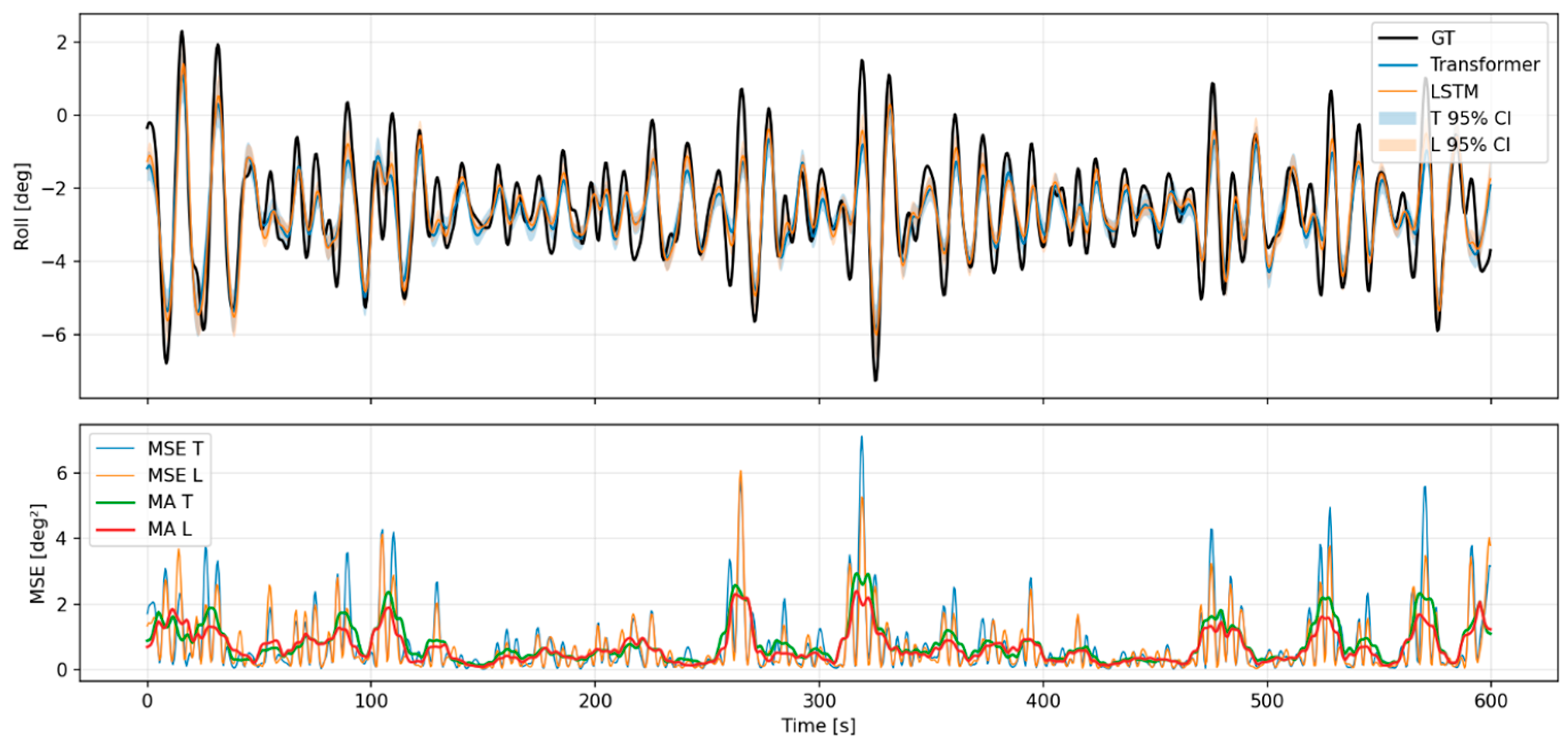
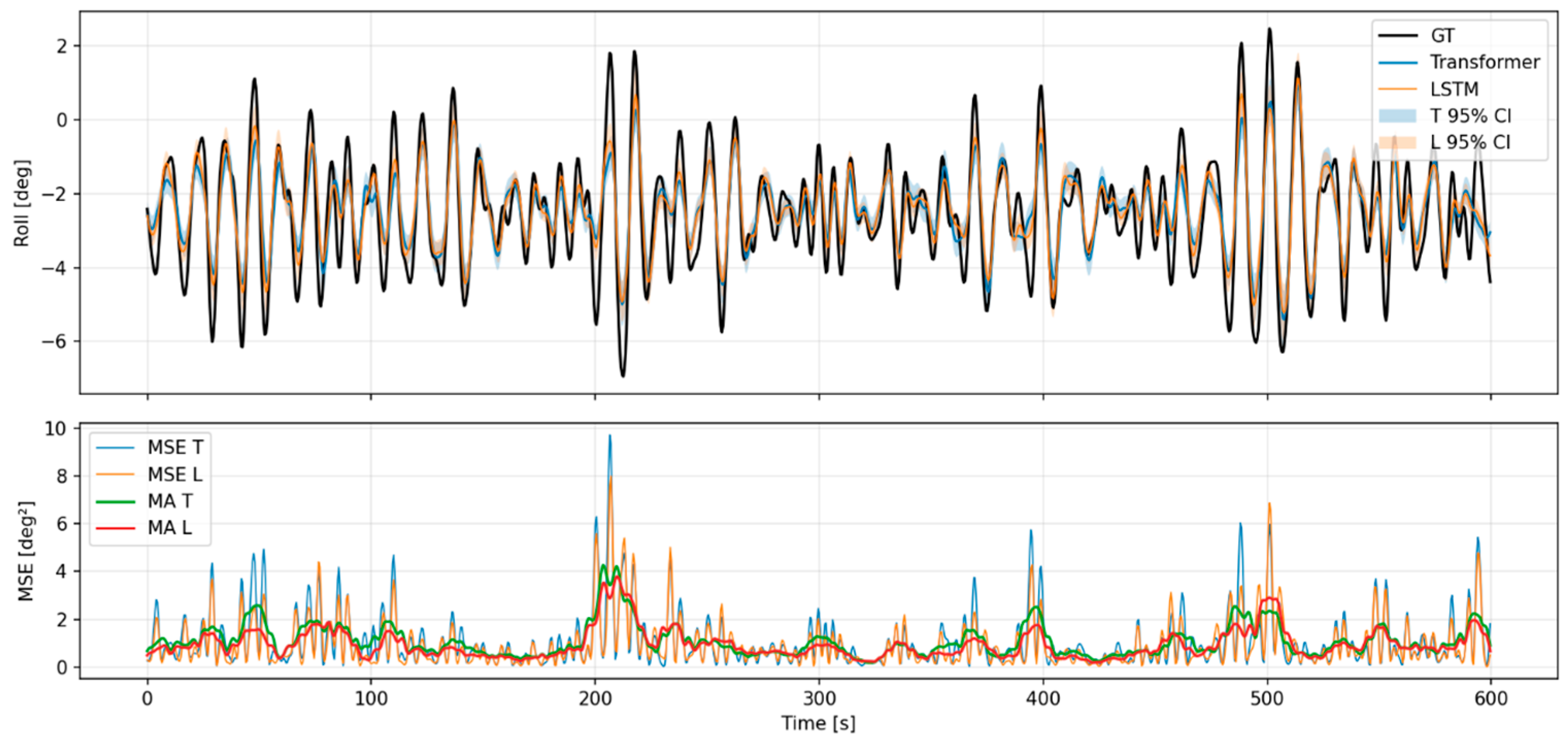
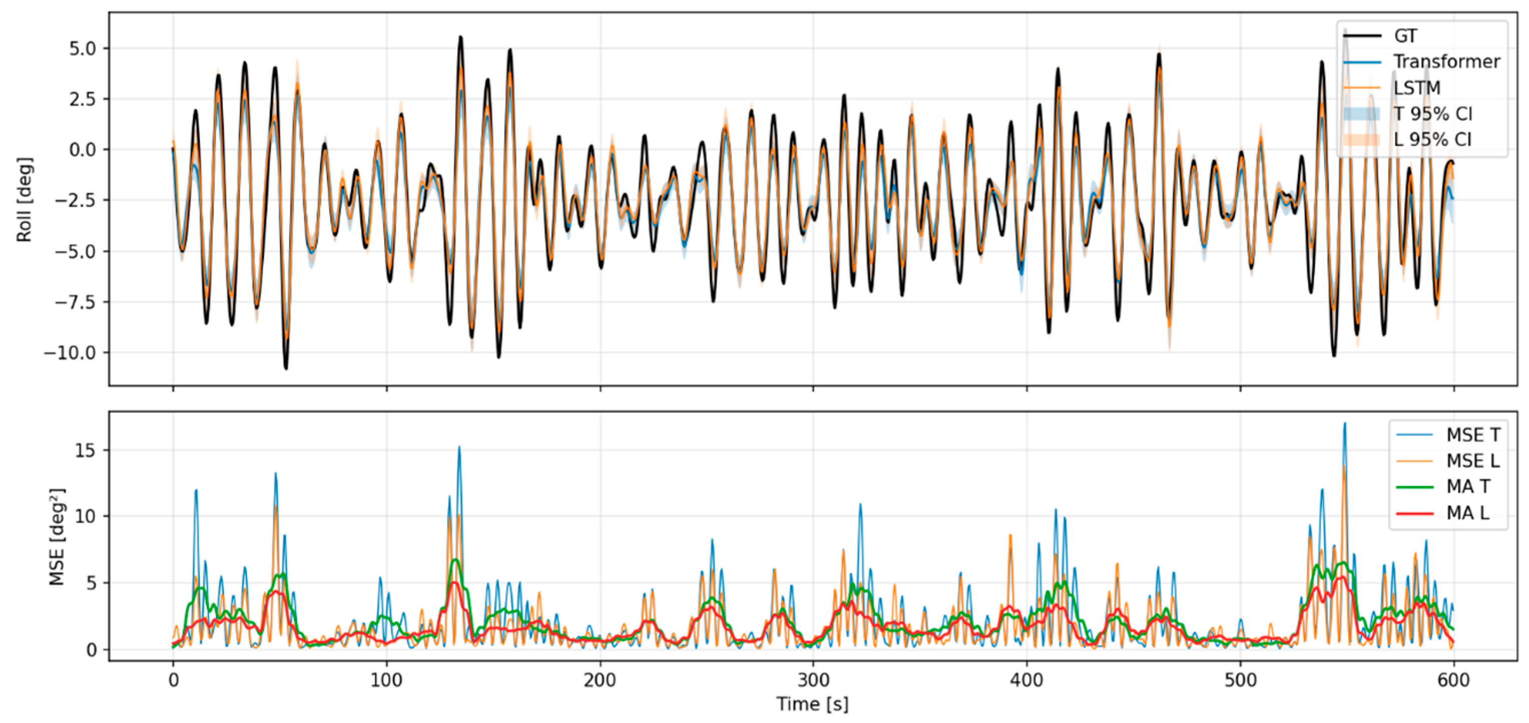
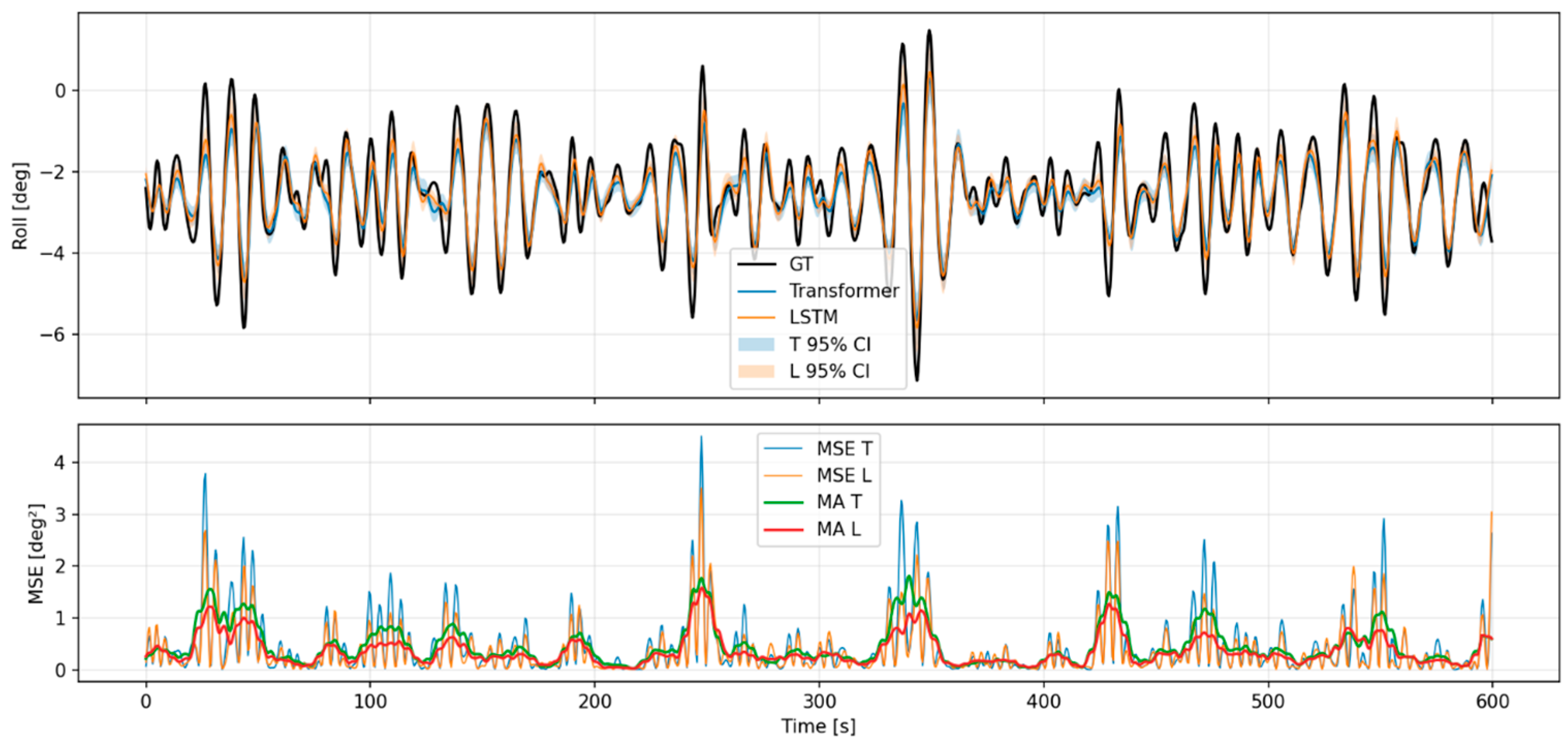
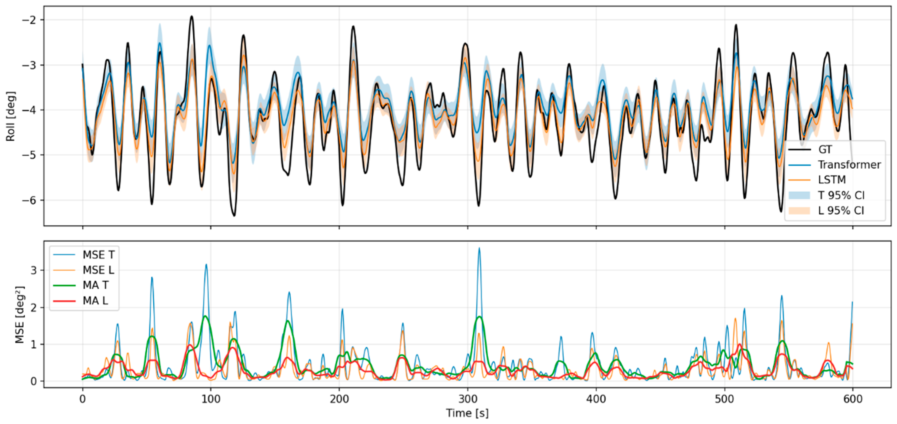
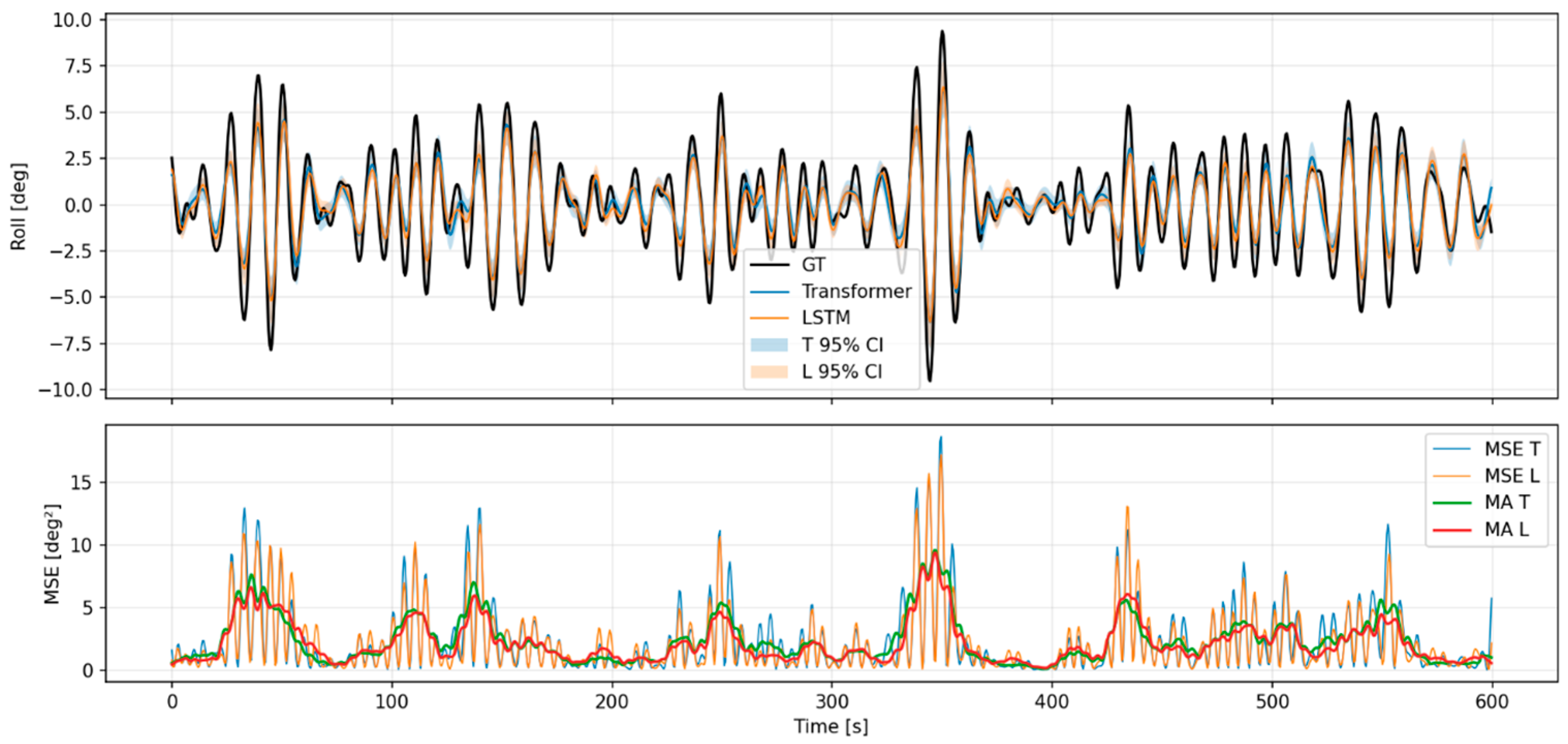
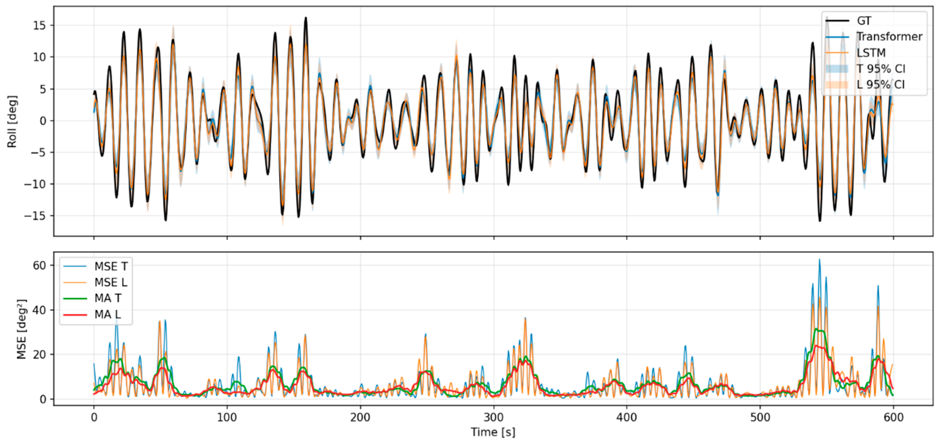
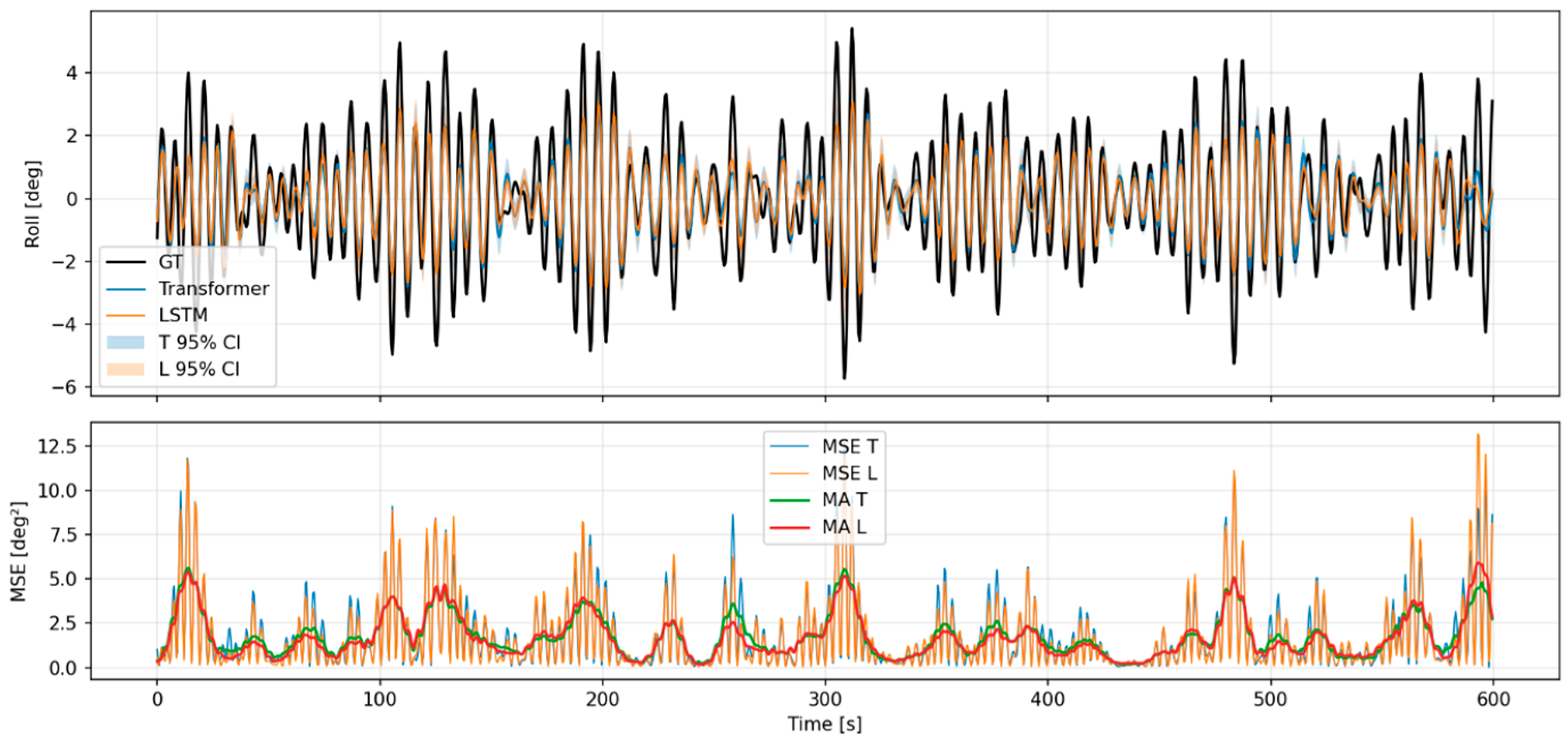
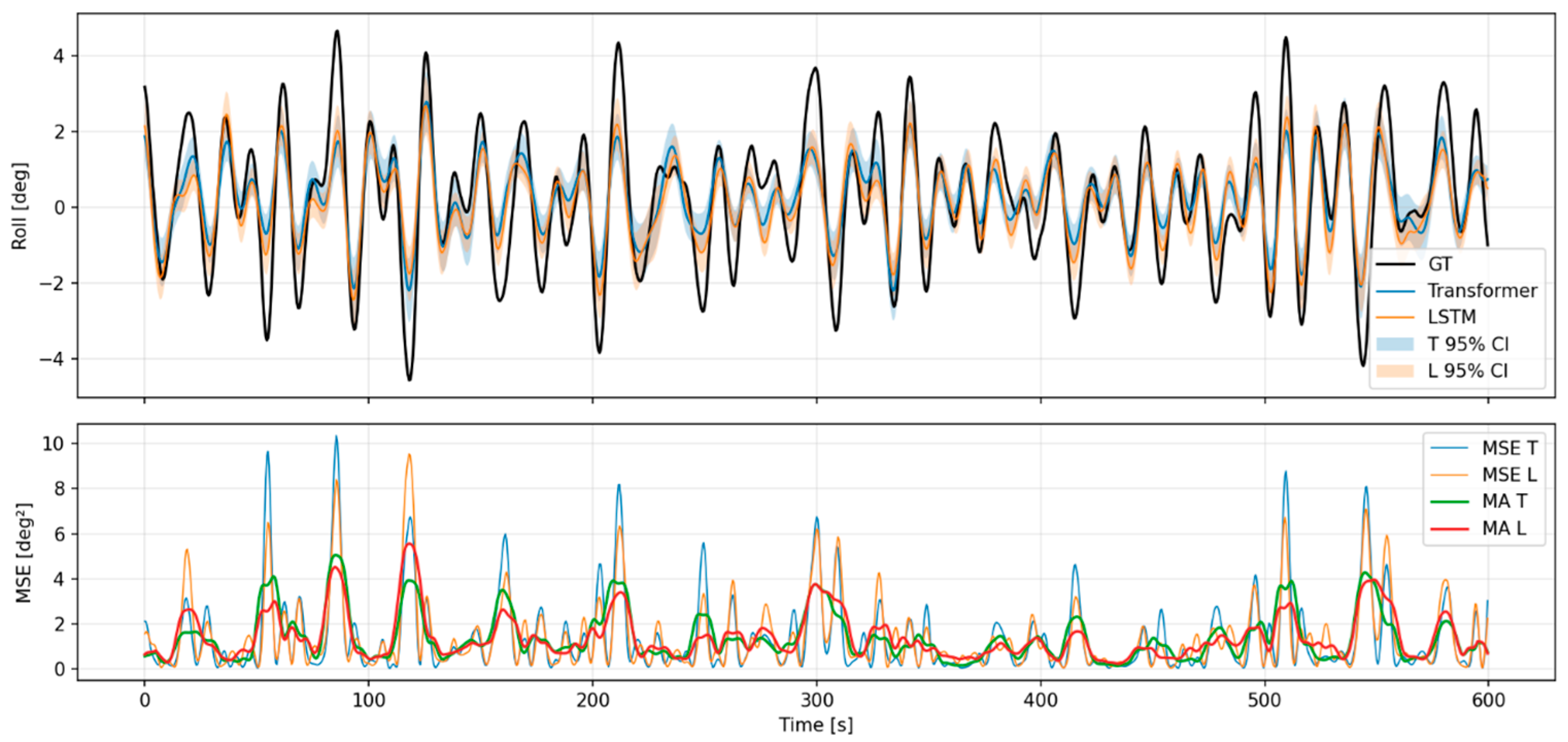
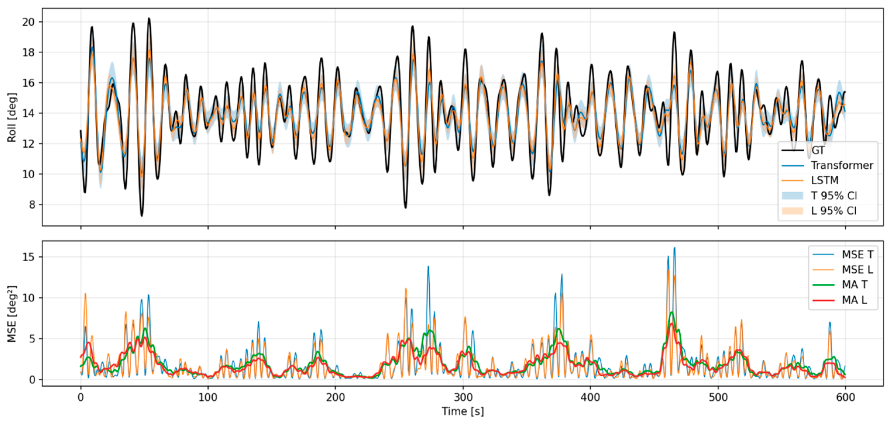
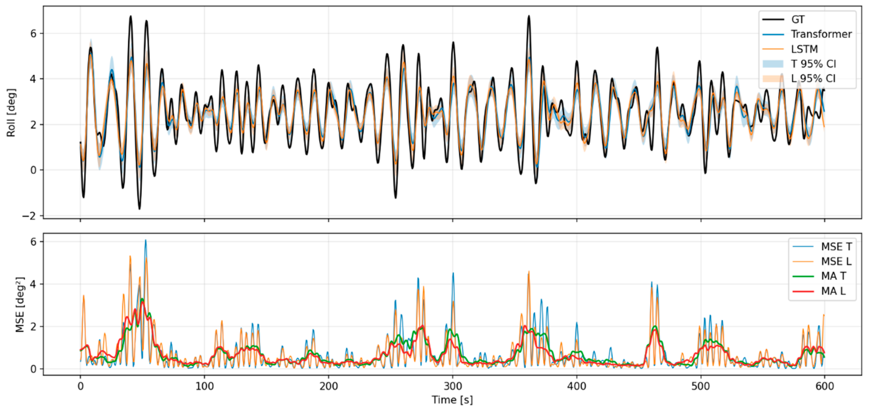
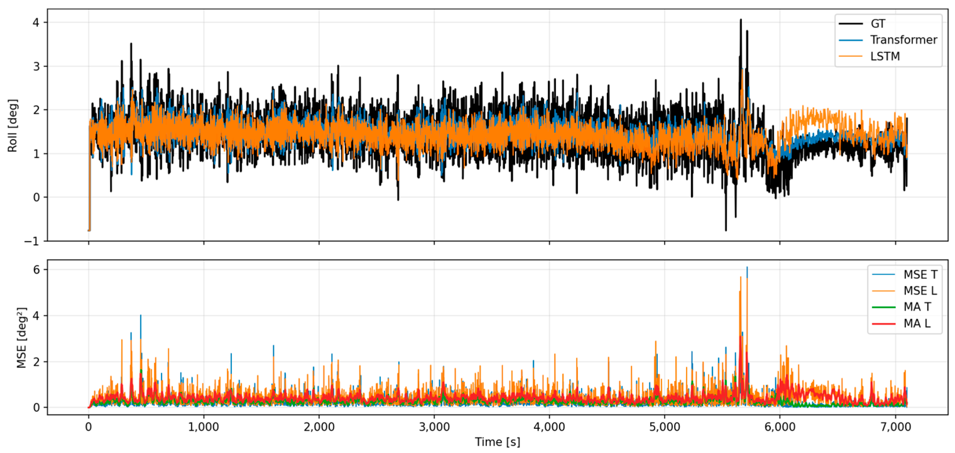
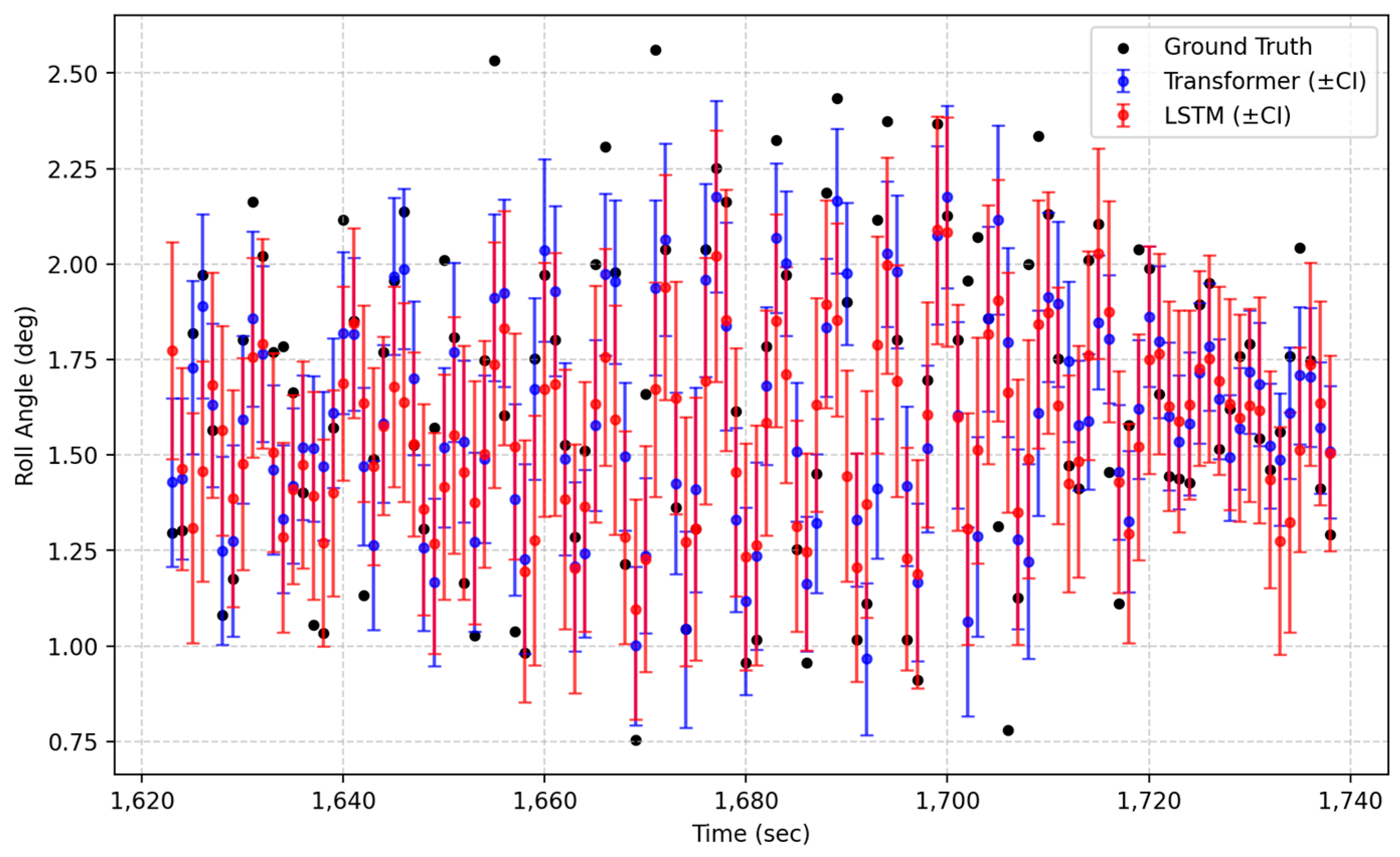
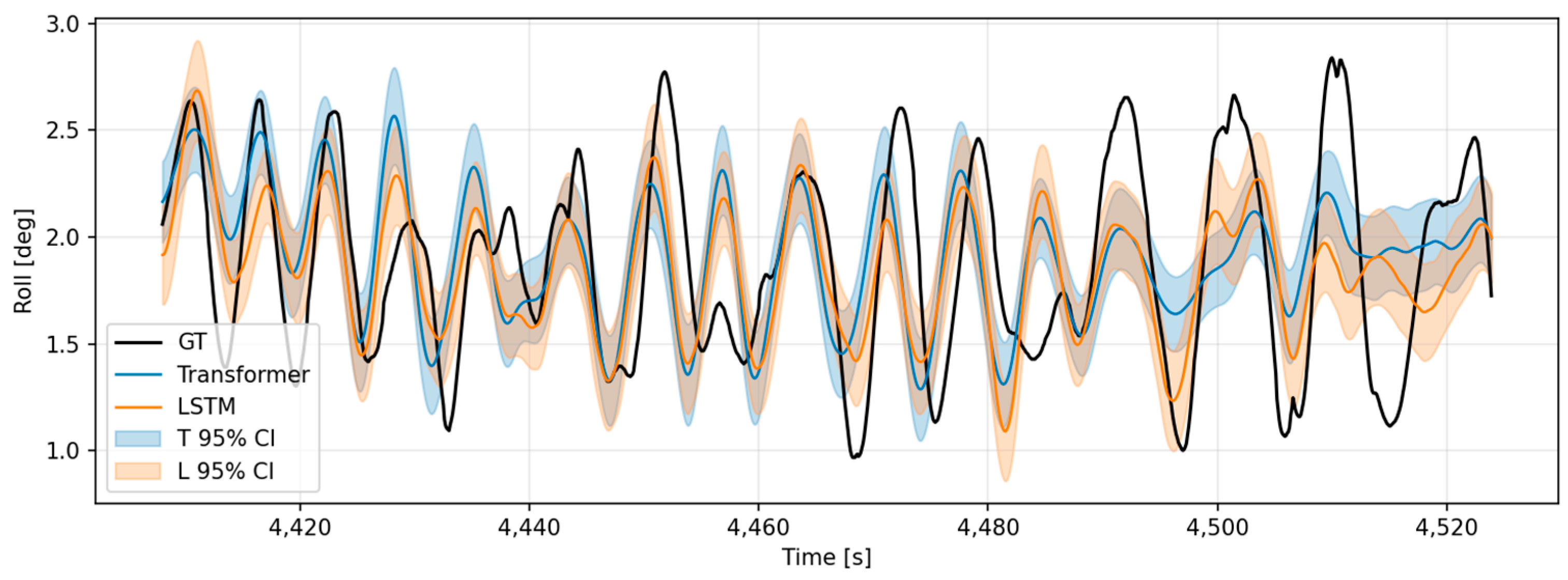
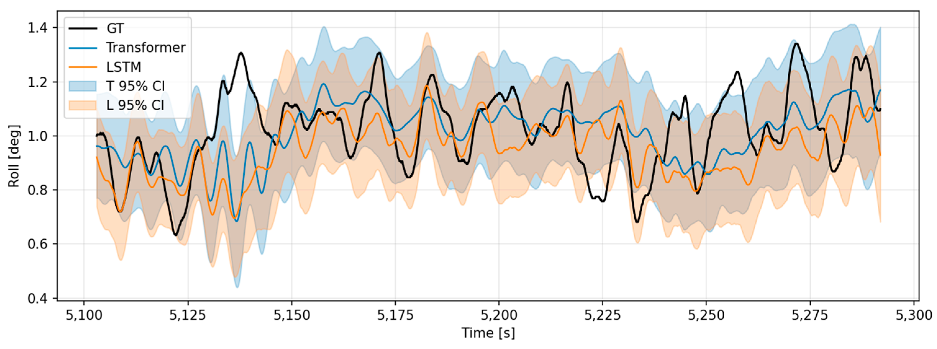
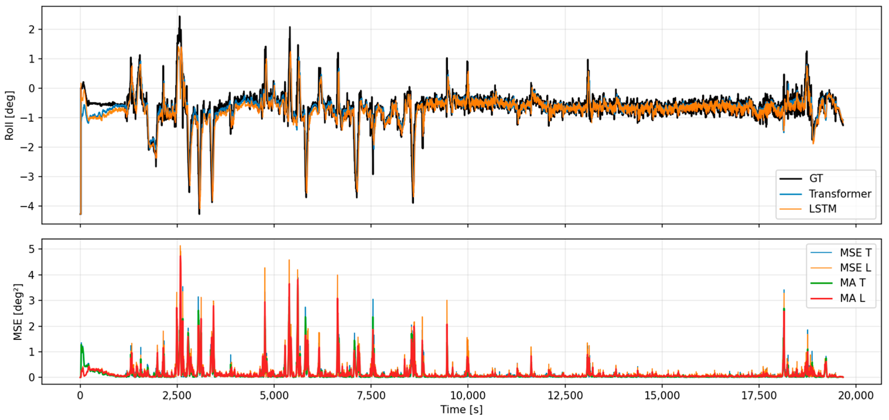
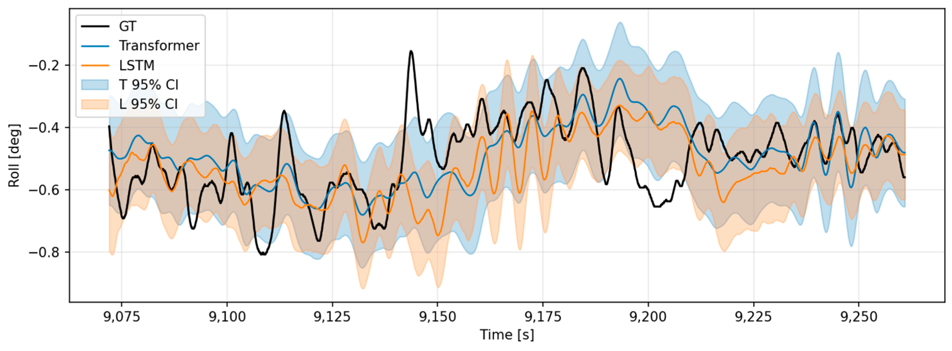
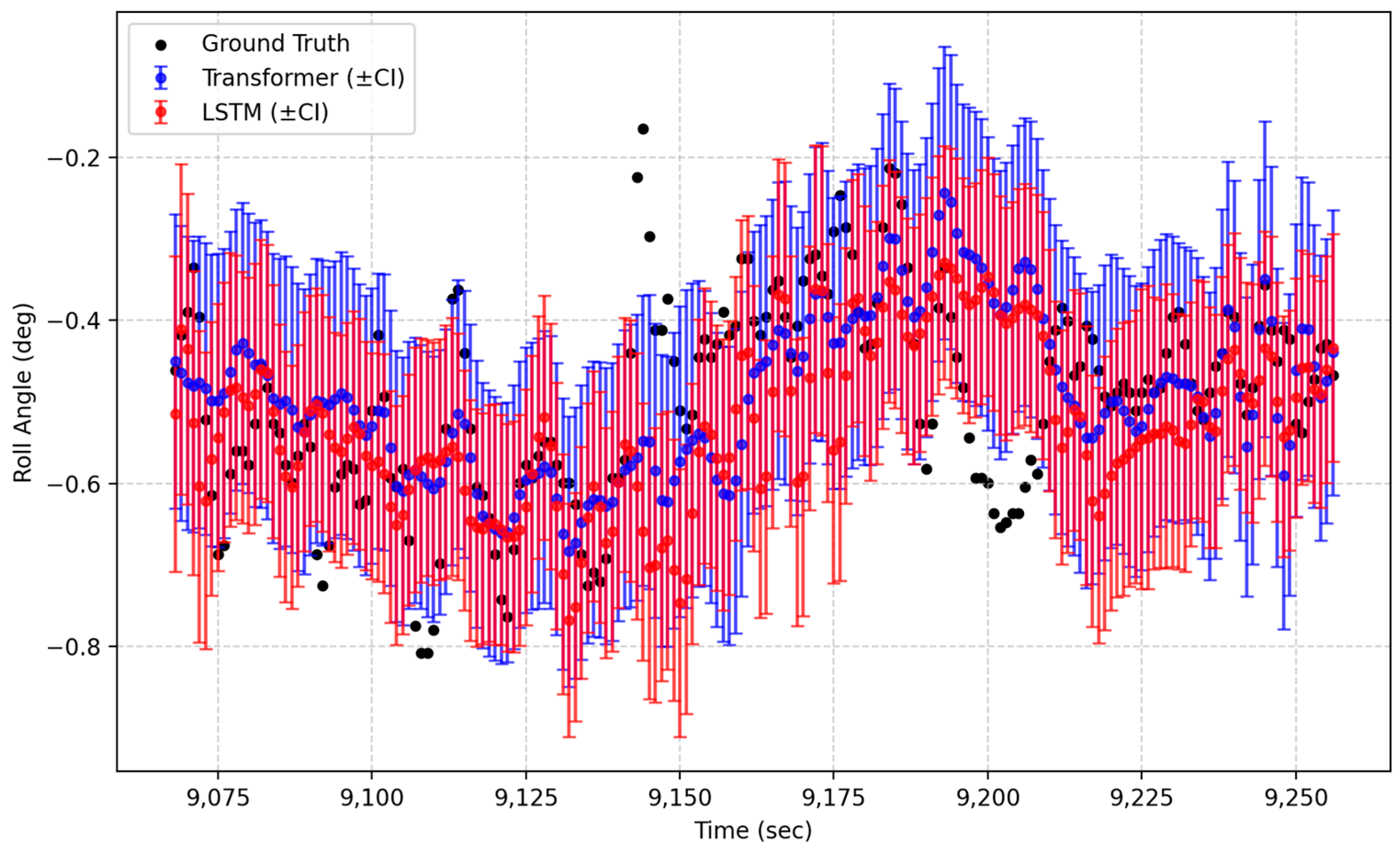
Figure 22, Figure 23, Figure 24, Figure 25, Figure 26, Figure 27, Figure 28, Figure 29, Figure 30, Figure 31, Figure 32 and Figure 33 present representative comparisons between the measured and predicted roll-motion time series for both ferries. Figure 22, Figure 25, Figure 28 and Figure 31 show the entire-sequence predictions, while Figure 23, Figure 26, Figure 29 and Figure 32 provide localized visualizations extracted from specific time segments of those sequences to highlight detailed variations in the predicted mean and variance obtained through Monte Carlo (MC) Dropout. Additionally, Figure 24, Figure 27, Figure 30 and Figure 33 illustrate the same prediction intervals using scatter-plot representations with error bars to depict the model-based uncertainty distributions at coarser temporal sampling rates.

In the full-sequence plots (Figure 22, Figure 25, Figure 28 and Figure 31), the upper panels illustrate the measured roll motions (black solid lines) together with the predicted trajectories produced by the Transformer (blue) and LSTM (orange) models. The shaded regions denote the 95% confidence intervals (mean ± 1.96 σ) derived from MC Dropout sampling, representing the predictive uncertainty of each model. From these results, the Transformer model demonstrates superior performance in reproducing the amplitude variations and phase alignment of the measured signals while maintaining narrower confidence intervals than the LSTM model. This indicates that the Transformer more effectively captures temporal dependencies in the time-series data and yields more stable probabilistic predictions.

The lower panels of each figure depict the point-wise mean-squared error (MSE) and its moving average (MA) for both models, providing insight into instantaneous prediction-error fluctuations and long-term accuracy trends. The comparative MSE–MA profiles quantitatively highlight the prediction stability and reliability of the Transformer model relative to the LSTM model. To further investigate local dynamics that are not clearly visible in the global plots, selected time segments were extracted and visualized separately: Segment 15/62 (t = 1624.0–1739.9 s) and 39/62 (t = 4408.0–4523.9 s) for Car Ferry A (Figure 23 and Figure 26), and Segment 28/81 (t = 5103.0–5291.9 s) and 49/105 (t = 9072.0–9260.9 s) for Car Ferry B (Figure 29 and Figure 32).

Complementary scatter-and-error-bar plots (Figure 24, Figure 27, Figure 30 and Figure 33) correspond to these local intervals, displaying the instantaneous predicted values from both models with their 95% confidence ranges at reduced temporal resolutions (Δt = 0.5–1.0 s). These figures visually emphasize how the Transformer and LSTM models express uncertainty across time while preserving the overall trend of the measured roll motion.

They reveal that the Transformer maintains smoother variance trends even under dynamically varying conditions, whereas the LSTM exhibits sharper variance spikes coinciding with transient roll peaks—reinforcing the complementary characteristics of deterministic accuracy (LSTM) and probabilistic stability (Transformer).

5. Conclusions

This study developed and validated a deep-learning framework for short-term ship roll motion prediction that explicitly quantifies epistemic uncertainty using Monte Carlo (MC) Dropout. Two representative architectures—Long Short-Term Memory (LSTM) and Transformer encoders—were trained on 384 HydroD–Wasim simulations and further validated with real-voyage measurements from two ferries to evaluate both deterministic accuracy and probabilistic reliability.

The results showed that the LSTM model consistently achieved lower mean squared errors (MSE) across all sea states, ship speeds, and loading conditions, demonstrating superior deterministic prediction capability. In contrast, the Transformer model exhibited higher Prediction Interval Coverage Probability (PICP) and wider Prediction Interval Normalized Average Width (PINAW), indicating more conservative and stable uncertainty estimation. These complementary characteristics suggest that the LSTM is advantageous for precise short-term motion forecasting, while the Transformer provides more reliable uncertainty representation and confidence calibration under diverse operational conditions.

The integration of MC Dropout proved to be an efficient Bayesian approximation method for quantifying model uncertainty without additional architectural modification or retraining. This approach successfully captured the reliability of deep-learning–based predictions, offering probabilistic insight into model confidence and error margins—an essential component for risk-aware maritime decision systems.

Validation using real-sea measurements confirmed that both models generalize well beyond simulated conditions. The Transformer showed slightly better performance under mild sea states, whereas the LSTM achieved higher accuracy under more dynamic roll responses. Moreover, a localized segment-wise visualization of the predictive mean and variance revealed that the Transformer maintains smoother uncertainty distributions, while the LSTM exhibits sharper sensitivity to transient roll peaks, reinforcing their complementary strengths in practical applications.

Overall, the findings demonstrate that deep-learning–based ship motion forecasting combined with uncertainty quantification can substantially enhance the safety, reliability, and interpretability of intelligent maritime systems. The proposed framework provides a robust foundation for real-time roll monitoring, onboard stability assessment, and predictive control in autonomous and remotely operated vessels. Furthermore, the demonstrated ability to characterize uncertainty and model the influence of unobserved factors suggests that the present results can serve as an initial step toward systematically analyzing external disturbances and their impact on vessel stability—an area that remains critical for advancing resilient control and safety assurance in future maritime operations.

Future work will train the model by adding a kinetic interpretation dataset under various vessels and conditions to improve generalization performance and improve prediction uncertainty. Another limitation identified in this study is that, although the actual ships employed rudder control during real-voyage operations, such control inputs were not included in the current learning models. Future work will address this limitation by incorporating rudder angle and steering dynamics as exogenous variables, thereby improving model fidelity and enhancing prediction accuracy under realistic maneuvering conditions.

References

1. Lee, H.; Ahn, Y. Comparative Study of RNN-Based Deep Learning Models for Practical 6-DOF Ship Motion Prediction. J. Mar. Sci. Eng. 2025, 13, 1792. [Google Scholar] [CrossRef]
2. Gao, N.; Chuang, Z.; Hu, A. Online Data-Driven Integrated Prediction Model for Ship Motion Based on Data Augmentation and Filtering Decomposition and Time-Varying Neural Network. J. Mar. Sci. Eng. 2024, 12, 2287. [Google Scholar] [CrossRef]
3. Guo, S.; Zhuang, S.; Wang, J.; Peng, X.; Liu, Y. Deep Learning-Based Non-Parametric System Identification and Interpretability Analysis for Improving Ship Motion Prediction. J. Mar. Sci. Eng. 2025, 13, 2017. [Google Scholar] [CrossRef]
4. Guo, Z.; Qiang, H.; Peng, X. Vessel Trajectory Prediction Using Vessel Influence Long Short-Term Memory with Uncertainty Estimation. J. Mar. Sci. Eng. 2025, 13, 353. [Google Scholar] [CrossRef]
5. Zhou, F.; Wang, S. A Hybrid Framework Integrating End-to-End Deep Learning with Bayesian Inference for Maritime Navigation Risk Prediction. J. Mar. Sci. Eng. 2025, 13, 1925. [Google Scholar] [CrossRef]
6. Xu, D.; Yin, J. Probabilistic Interval Prediction of Ship Roll Motion Using Multi-Resolution Decomposition and Non-Parametric Kernel Density Estimation. J. Mar. Sci. Appl. 2025, 24, 1–12. [Google Scholar] [CrossRef]
7. Xu, D.-X.; Yin, J.-C. Real-Time Ship Roll Prediction via a Novel Stochastic Trainer-Based Feedforward Neural Network. China Ocean Eng. 2025, 39, 608–620. [Google Scholar] [CrossRef]
8. Capobianco, S.; Forti, N.; Millefiori, L.M.; Braca, P.; Willett, P. Recurrent Encoder-Decoder Networks for Vessel Trajectory Prediction with Uncertainty Estimation. J. Mar. Sci. Eng. 2022, 10, 103222. [Google Scholar] [CrossRef]
9. Lu, Z.-F.; Yan, H.-C.; Xu, J.-B. A Heave Motion Prediction Approach Based on Sparse Bayesian Learning Incorporated with Empirical Mode Decomposition for an Underwater Towed System. J. Mar. Sci. Eng. 2025, 13, 1427. [Google Scholar] [CrossRef]
10. Fan, G.-J.; Yu, P.-Y.; Wang, Q.; Dong, Y.-K. Short-Term Motion Prediction of a Semi-Submersible by Combining LSTM Neural Network and Different Signal Decomposition Methods. Ocean Eng. 2023, 267, 113266. [Google Scholar] [CrossRef]
11. Li, S.-Y.; Wang, T.-T.; Li, G.-Y.; Skulstad, R.; Zhang, H.-X. Short-Term Ship Roll Motion Prediction Using the Encoder–Decoder Bi-LSTM with Teacher Forcing. Ocean Eng. 2024, 295, 116917. [Google Scholar] [CrossRef]
12. Zhang, T.; Zheng, X.-Q.; Liu, M.-X. Multiscale Attention-Based LSTM for Ship Motion Prediction. Ocean Eng. 2021, 230, 109066. [Google Scholar] [CrossRef]
13. Silva, K.M.; Maki, K.J. Data-Driven System Identification of 6-DoF Ship Motion in Waves with Neural Networks. Appl. Ocean Res. 2022, 125, 103222. [Google Scholar] [CrossRef]
14. Tian, J.; Song, S. Machine Learning for Short-Term Prediction of Ship Motion Combined with Wave Input. J. Mar. Sci. Eng. 2023, 11, 571. [Google Scholar] [CrossRef]
15. Sun, J.; Zeng, D.; Liu, H. Short-Term Ship Motion Attitude Prediction Based on LSTM and GPR. J. Ocean Res. 2022, 21, 1004–1012. [Google Scholar] [CrossRef]
16. Jiang, Z.; Ma, Y.; Li, W. A Data-Driven Method for Ship Motion Forecast. J. Mar. Sci. Eng. 2024, 12, 291. [Google Scholar] [CrossRef]
17. Shen, W.; Hu, X.; Liu, J.; Li, S.; Wang, H. A Pre-Trained Multi-Step Prediction Informer for Ship Motion Prediction with a Mechanism-Data Dual-Driven Framework. Eng. Appl. Artif. Intell. 2025, 139, 109523. [Google Scholar] [CrossRef]
18. Kim, S.; Lim, J. Prediction for Ship Roll Motion by Stacked Deep Learning Model. JKIIS 2023, 33, 320–335. [Google Scholar] [CrossRef]
19. DNV GL AS. Feature Description Software Suite for Hydrodynamic and Structural Analysis of Ships and Offshore Structures. DNV GL—Digital Solutions, 2020. Available online: https://share.google/PBITu308WJ8jzG4Of (accessed on 1 December 2025).
20. DNV. Hydrodynamic Analysis and Stability Analysis Software—HydroD. Available online: https://www.dnv.com/services/hydrodynamic-analysis-and-stability-analysis-software-hydrod-14492/ (accessed on 1 December 2025).
21. Greff, K.; Srivastava, R.K.; Koutník, J.; Steunebrink, B.R.; Schmidhuber, J. LSTM: A Search Space Odyssey. IEEE Trans. Neural Netw. Learn. Syst. 2017, 28, 2222–2232. [Google Scholar] [CrossRef]
22. Hochreiter, S.; Schmidhuber, J. Long Short-Term Memory. Neural Comput. 1997, 9, 1735–1780. [Google Scholar] [CrossRef]
23. Vaswani, A.; Shazeer, N.; Parmar, N.; Uszkoreit, J.; Jones, L.; Gomez, A.N.; Kaiser, Ł.; Polosukhin, I. Attention Is All You Need. Adv. Neural Inf. Process. Syst. 2017, 30, 5998–6008. [Google Scholar]
24. Devlin, J.; Chang, M.-W.; Lee, K.; Toutanova, K. BERT: Pre-training of Deep Bidirectional Transformers for Language Understanding. In Proceedings of the 2019 Conference of the North American Chapter of the Association for Computational Linguistics: Human Language Technologies, Minneapolis, MN, USA, 2–7 June 2019; pp. 4171–4186. [Google Scholar]
25. Shaw, P.; Uszkoreit, J.; Vaswani, A. Self-Attention with Relative Position Representations. In Proceedings of the 2018 Conference of the North American Chapter of the Association for Computational Linguistics: Human Language Technologies, New Orleans, LA, USA, 1–6 June 2018; pp. 464–468. [Google Scholar]
26. Der Kiureghian, A.; Ditlevsen, O. Aleatory or epistemic? Does it matter? Struct. Saf. 2009, 31, 105–112. [Google Scholar] [CrossRef]
27. Kendall, A.; Gal, Y. What uncertainties do we need in Bayesian deep learning for computer vision? In Advances in Neural Information Processing Systems 30 (NIPS 2017); Springer: Cham, Switzerland, 2017; pp. 5574–5584. [Google Scholar]
28. Gal, Y.; Ghahramani, Z. Dropout as a Bayesian Approximation: Representing Model Uncertainty in Deep Learning. In Proceedings of the 33rd International Conference on Machine Learning (ICML 2016), New York, NY, USA, 20–22 June 2016; Volume 48, pp. 1050–1059. [Google Scholar]
Figure 1. Car Ferry A (a) and B (b) roll time series data.
Jmse 13 02378 g001
Figure 2. Location of Chujado Marine Meteorological buoy (red circle).
Jmse 13 02378 g002
Figure 3. Heatmap of wave period versus significant wave height at Chujado, Jeju.
Jmse 13 02378 g003
Figure 4. Histogram of wave direction distribution at Chujado buoy.
Jmse 13 02378 g004
Figure 5. GEV fit to wave-height distribution (100-year return level).
Jmse 13 02378 g005
Figure 6. Car Ferry A PLN (a) and panel (b) model (HydroD).
Jmse 13 02378 g006
Figure 7. Car Ferry B PLN (a) and panel (b) model (HydroD).
Jmse 13 02378 g007
Figure 8. HydroD-Wasim time-domain motion-analysis results (Car Ferry A).
Jmse 13 02378 g008
Figure 9. Dataset partitioning for time-series data (train, validation, and test).
Jmse 13 02378 g009
Figure 10. Classification of uncertainty types (aleatoric vs. epistemic). The spread of data points reflects aleatoric uncertainty, with wide dispersion indicating high noise and narrow dispersion indicating low noise. Regions lacking training data—such as the central interval—exhibit high epistemic uncertainty due to limited model knowledge.
Jmse 13 02378 g010
Figure 11. Principle of MC Dropout—repeated stochastic inference generates a predictive distribution and confidence interval from the same input.
Jmse 13 02378 g011
Figure 12. Effect of significant wave height on prediction accuracy and uncertainty (Car Ferry A).
Jmse 13 02378 g012
Figure 13. Effect of mean wave period on prediction accuracy and uncertainty (Car Ferry A).
Jmse 13 02378 g013
Figure 14. Effect of wave direction on prediction accuracy and uncertainty (Car Ferry A).
Jmse 13 02378 g014
Figure 15. Effect of ship speed on prediction accuracy and uncertainty (Car Ferry A).
Jmse 13 02378 g015
Figure 16. Effect of loading and damage conditions on prediction accuracy and uncertainty (Car Ferry A).
Jmse 13 02378 g016
Figure 17. Effect of significant wave height on prediction accuracy and uncertainty (Car Ferry B).
Jmse 13 02378 g017
Figure 18. Effect of mean wave period on prediction accuracy and uncertainty (Car Ferry B).
Jmse 13 02378 g018
Figure 19. Effect of wave direction on prediction accuracy and uncertainty (Car Ferry B).
Jmse 13 02378 g019
Figure 20. Effect of ship speed on prediction accuracy and uncertainty (Car Ferry B).
Jmse 13 02378 g020
Figure 21. Effect of loading and damage conditions on prediction accuracy and uncertainty (Car Ferry B).
Jmse 13 02378 g021
Figure 22. Predicted roll motion of Car Ferry A (from Jeju; Hs = 1.4 m, Tz = 4.9 s, Dir = 85°, U = 10.5 m/s, L/C = Static).
Jmse 13 02378 g022
Figure 23. Predicted roll motion of Car Ferry A (from Jeju)—Segment 15/62 (t = 1624.0–1739.9 s).
Jmse 13 02378 g023
Figure 24. Scatter plot of Transformer and LSTM roll motion predictions with 95% confidence intervals of Car Ferry A (from Jeju, t = 1623.0–1738.0 s, sampled at Δt = 1.0 s).
Jmse 13 02378 g024
Figure 25. Predicted roll motion of Car Ferry A (to Jeju; Hs = 1.3 m, Tz = 4.2 s, Dir = 96°, U = 10.8 m/s, L/C = Static).
Jmse 13 02378 g025
Figure 26. Predicted roll motion of Car Ferry A (to Jeju)—Segment 39/62 (t = 4408.0~4523.9 s).
Jmse 13 02378 g026
Figure 27. Scatter plot of Transformer and LSTM roll motion predictions with 95% confidence intervals of Car Ferry A (to Jeju, t = 4404.0–4520.0 s, sampled at Δt = 1.0 s).
Jmse 13 02378 g027
Figure 28. Predicted roll motion of Car Ferry B (from Jeju; Hs = 0.6 m, Tz = 6.4 s, Dir = 142°, U = 11.3 m/s, L/C = Static).
Jmse 13 02378 g028
Figure 29. Predicted roll motion of Car Ferry B (from Jeju)—Segment 28/81 (t = 5103.0~5291.9 s).
Jmse 13 02378 g029
Figure 30. Scatter plot of Transformer and LSTM roll motion predictions with 95% confidence intervals of Car Ferry B (from Jeju, t = 5100.0–5289.0 s, sampled at Δt = 1.0 s).
Jmse 13 02378 g030
Figure 31. Predicted roll motion of Car Ferry B (to Jeju; Hs = 0.4 m, Tz = 5.0 s, Dir = 17°, U = 9.7 m/s, L/C = Static).
Jmse 13 02378 g031
Figure 32. Predicted roll motion of Car Ferry B (to Jeju)—segment 49/105 (t = 9072.0~9260.9 s).
Jmse 13 02378 g032
Figure 33. Scatter plot of Transformer and LSTM roll motion predictions with 95% confidence intervals of Car Ferry B (to Jeju, t = 9067.0–9256.0 s, sampled at Δt = 1.0 s).
Jmse 13 02378 g033