Underwater Sound Source Depth Estimation Using Deep Learning and Vector Acoustic Features

Abstract

Accurate estimation of underwater sound source depth plays a crucial role in ocean acoustic monitoring, underwater target localization, and marine environment exploration. This study exploits the capability of vector hydrophones to simultaneously and co-locally acquire both scalar and vector components of the underwater sound field. Based on the study of the line spectrum interference structure characteristics of the underwater sound field, the vertical sound intensity flux of the underwater sound source is extracted. Additionally, a parallel BiLSTM and ResNet network structure is proposed to train this feature and achieve depth estimation of underwater sound sources. Experimental results show that under ±10% and ±15% errors in the source–hydrophone distance, the proposed model maintains stable performance within a signal-to-noise ratio (SNR) range of −15 dB to +15 dB. Compared with the LSTM model, the ResNet model, and the matched-field processing (MFP) algorithm, the average RMSE of our model is reduced by 72.4%, 54.0%, and 64.1%, respectively. Furthermore, under 5% and 10% frequency estimation errors, the average RMSE of the proposed model within the same SNR range is reduced by 47.7%, 20.3%, and 79.3%, respectively. It effectively estimates the depth of underwater sound sources, with estimation errors below 5 m under non-extreme SNR conditions. These results fully demonstrate the robustness and effectiveness of the proposed method under practical uncertainties in the ocean environment.

1. Introduction

With the rapid development of underwater combat and marine intelligent equipment, underwater navigation devices are facing higher requirements for their ability to detect, locate, and identify targets [1]. To ensure their concealment and safety, such devices typically use passive acoustic methods to obtain environmental information. Among the various parameters, the depth of an underwater sound source is critical for accurate positioning and target classification, and its estimation accuracy directly influences overall system performance. Therefore, developing a depth estimation method with high reliability and robustness is of significant importance for enhancing the intelligent perception and decision-making capabilities of underwater vehicles.

Currently, depth estimation methods based on sound pressure hydrophones remain the mainstream approach. Li H et al. proposed a method to estimate the distance and depth of sound source simultaneously by using a vertical array deployed on the deep seabed. This method combines the angle of arrival of the direct wave and the interference characteristics generated by the direct wave and the sea-bottom reflection wave, and realises one-step inferential positioning and depth measurement [2]. At the same time, Kniffin et al. systematically investigated the algorithmic stability and applicability range of passive depth estimation based on the Generalised Fourier Transform (GFT). This method relies on the interference structure formed between direct waves and sea surface-seabed reflected waves to accurately estimate the source depth [3]. Emmettiere uses a horizontal array to address the issue of determining the depth attributes of sound sources in deep-sea environments. It is pointed out that under far-field low-frequency broadband conditions, waveguide invariants are highly correlated with sound source depth and can be used for depth determination. McCargar and Zurk introduced a physical FT variant, leveraging the depth modulation characteristics of direct waves and sea surface reflection waves to achieve passive signal depth separation and estimation without requiring environmental prior knowledge [4]. In shallow water environments, Byun et al. compared the localisation performance of array invariant-based and matched field processing methods. The results showed that when the array tilt angle is unknown, or the environmental model contains errors, the AI method exhibits stronger robustness and self-calibration capabilities. After compensating for the array tilt angle, MFP can approach the performance of AI in range estimation, but this requires a highly accurate environmental model [5]. Scalar hydrophones can only detect sound pressure signals and cannot obtain directional information about sound wave propagation, resulting in limited perception capabilities of the propagation paths and normalised wave mode characteristics [6]. Estimation accuracy is highly sensitive to changes in the marine environment, and the low input feature dimension is unfavourable for the construction and generalisation capability of deep learning models. Especially in complex shallow sea and low SNR environments, the performance of traditional methods is further constrained. In contrast, vector hydrophones, which can simultaneously acquire both sound pressure and particle velocity signals, offer higher information dimensions and directional sensitivity, making them an important development direction in underwater acoustic detection technology in recent years. Currently, there has been extensive research and application of vector hydrophones and vector signal processing technology in azimuth estimation. In recent years, the field of underwater depth estimation has developed rapidly. Rong et al. proposed a time-series estimation method based on interference pattern flow sequences, effectively addressing moving sound sources and frequency errors [7]. The line spectrum interference structure in the sound field is highly sensitive to frequency, and the interference fringes formed by the superposition of different modes can serve as important physical features for determining the depth attributes of sound sources and estimating depth. Hui Junying et al. proposed an algorithm for determining the depth attributes of targets in the very low-frequency band using the characteristics of line spectrum interference structures [8]. Shi proposed a depth classification method based on the cross-spectral distribution of sound pressure and horizontal particle velocity in the normal mode. This method is effective only when the first two normal modes are excited in the very low-frequency band and determines the target category by setting a critical depth [9]. Subsequently, Zhao extended this principle to the low-order mode region of the vertical vector intensity, achieving depth classification and improved robustness over a wider frequency band [10]. Domestic and international research indicates that the vector acoustic features provided by vector hydrophones have a significant advantage in reflecting the acoustic field structure. If combined with modern machine learning methods, this could significantly improve the accuracy and robustness of underwater sound source depth estimation. In recent years, deep learning methods have demonstrated powerful capabilities in the field of underwater sound source localisation [11]. Compared with traditional matched field processing (MFP) methods, deep learning can approximate complex nonlinear relationships without the need for precise environmental modelling and has strong noise resistance and generalisation performance. For example, Wenbo Wang et al. constructed an interference spectrum using low spatial frequency interference maps and combined it with an improved CNN architecture, significantly improving depth prediction accuracy [12]; Amir Weiss and Toros Arikan proposed an end-to-end convolutional neural network architecture, DLOC (Data-Driven Direct Localisation), which enables fast sound source localisation inference without relying on environmental prior information. Under multi-path propagation and high-noise conditions, this model demonstrates excellent robustness and inference efficiency, with performance approaching that of optimal model-driven methods [13].

In summary, although there has been considerable research on underwater sound source localization, most studies still rely on traditional scalar hydrophones and their associated algorithms. Compared with vector hydrophones, scalar hydrophones lack particle velocity information in different directions, which limits the stability of underwater sound field construction in complex environments and easily leads to environmental mismatches, resulting in depth estimation errors. In addition, current studies require high accuracy of prior information, such as the source–hydrophone distance and source frequency; when errors exist in distance or frequency measurements, the depth estimation accuracy can be significantly affected.

To address these limitations, this study proposes a depth estimation framework for underwater sound sources based on vector acoustic features, integrating BiLSTM and ResNet modules. In Section 2.1, through research and analysis of the interference structure characteristics of the marine acoustic field, the active component of the vertical complex sound intensity is selected as the key input feature. This feature, composed of sound pressure and vertical particle velocity, can represent the vertical propagation direction of sound energy in water and offers stronger depth discrimination capabilities [14,15,16]. Comparative simulation analyses further demonstrate the superiority of this feature over other features. In Section 2.3, to fully exploit the local information and spatial patterns within this feature, a fusion neural network architecture combining ResNet1D with a parallel bidirectional BiLSTM is designed. This structure simultaneously possesses the deep feature representation capability of residual networks and the temporal modeling capability of recurrent networks, effectively enhancing the model’s adaptability to complex acoustic field variations and its depth estimation accuracy. Section 3 validates the proposed method using experimental simulation data, showing excellent performance and robustness under various marine environments and different SNR conditions, thereby providing a novel and effective technical approach for underwater intelligent sensing.

2. Methods and Feature Verification

2.1. Theoretical Basis

Vector acoustic features refer to multi-dimensional acoustic field information collected using vector hydrophones, encompassing both scalar components (sound pressure) and vector components (particle velocity). Compared to traditional sound pressure measurement methods, vector acoustic features provide a more comprehensive description of underwater acoustic field structures. With the continuous development of vector hydrophone technology, vector acoustic features have demonstrated significant application potential in fields such as underwater target localisation, depth estimation, direction identification, and target recognition [17]. In this paper, to accurately characterise the underwater multipath propagation characteristics and interference structure, a three-layer medium model (seawater layer, sediment layer, and semi-infinite bottom layer) is used as the basis for modelling and simulating the underwater acoustic field using normal mode theory. The normalised wave model can effectively analyse the propagation behaviour of each modal order at different depths and frequencies, making it particularly suitable for describing the complex vertical propagation structure in marine waveguide environments. By numerically solving the modal functions of sound waves under boundary conditions, the sound pressure and particle velocity in the simulated underwater sound field are obtained, providing theoretical support for interference feature extraction and sound source depth estimation. In the three-layer medium model, it is assumed that both the seawater layer and the sediment layer are homogeneous media, with constant sound velocity and medium density in each layer. The model is shown in Figure 1.

Vector Sound Field Calculation Model Based on Normalised Wave Theory

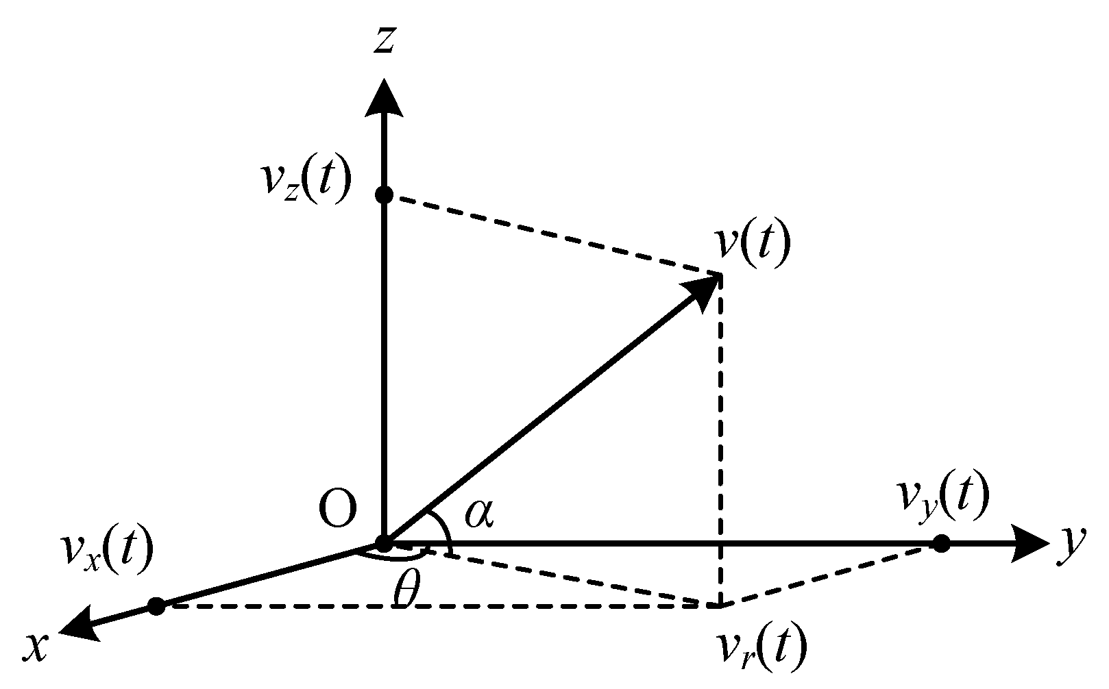
The vector hydrophone outputs sound pressure and orthogonal three-dimensional velocity components. The sound pressure signal $p(t)=x(t)$, where $x(t)$ is the target signal. The velocity signal $v(t)$ contains three orthogonal components:

$$v(t)=\left[\begin{array}{c}{v}_x(t)\\ v_y(t)\\ v_z(t)\end{array}\right]=\left[\begin{array}{c}{v}_r(t)\cos \theta \\ v_r(t)\sin \theta \\ v_z(t)\end{array}\right]=\left[\begin{array}{c}\cos \theta \cos \alpha \\ \sin \theta \cos \alpha \\ \sin \alpha \end{array}\right]{\displaystyle \frac{1}{{\rho }_1{c}_1}}x(t)$$

(1)

The geometric relationship between orthogonal components is shown in Figure 2. $\theta$ is the horizontal angle (range: 0° to 360°), with the positive direction of the x-axis being 0°, and $\alpha$ is the elevation angle (range: −90° to 90°), with the horizontal plane (xoy plane) being 0°.

The velocity potential $\phi$ of the underwater acoustic field excited by a target satisfies the wave equation:

$${\displaystyle \frac{1}{r}}{\displaystyle \frac{\partial }{\partial r}}(r{\displaystyle \frac{\partial \phi }{\partial r}})+{\displaystyle \frac{{\partial }^2\phi }{\partial z^2}}+k_i^2\phi =Q(r,z_0)$$

(2)

where $k_i={\displaystyle \frac{w}{c_i}},(i=0,1,2)$. In the medium layer containing the sound source $Q(r,z_0)=-4\pi \delta (r,z-z_0)$.

The expression for the velocity potential $\phi$ of the sound field excited by an underwater target in the water layer is given by:

$$\phi (r,z)={\displaystyle \sum _n\frac{2\pi j{\beta }_{1n}\sin ({\beta }_{1n}z)\sin ({\beta }_{1n}{z}_0)}{{\beta }_{1n}H-\sin ({\beta }_{1n}H)\cos ({\beta }_{1n}H)-b^2\tan ({\beta }_{1n}H){\sin }^2({\beta }_{1n}H)}}{H}^{(2)}({\xi }_{n}r)$$

(3)

where ${\beta }_i=\sqrt{k_i^2-{\xi }^2}$, $\xi$ represents the radial wavenumber. $b={\rho }_1/{\rho }_2$, ${\rho }_1$ denotes the density of the water layer, and ${\rho }_2$ denotes the density of the sediment layer. $H$ represents the water depth.

The sound pressure and particle velocity satisfy $p=\rho (\partial \phi /\partial t)$, $v_r=-(\partial \phi /\partial r)$, $v_z=-(\partial \phi /\partial z)$, so the expressions for the sound pressure field and vertical vibration velocity field excited by underwater targets received by underwater sensors in layered media [18] are:

$$P(z_0,z,r)=e^{j{\displaystyle \frac{\pi }{4}}}\sqrt{{\displaystyle \frac{8\pi }{r}}}\omega {\rho }_1{\displaystyle \sum _n\sqrt{\frac{1}{{\xi }_n}}{F}_n({\xi }_n){\mathsf{\Psi }}_n(z_0){\mathsf{\Psi }}_n(z)e^{-j{\xi }_{n}r}}$$

(4)

$$V_z(z_0,z,r)=-j{e}^{j{\displaystyle \frac{\pi }{4}}}\sqrt{{\displaystyle \frac{8\pi }{r}}}{\displaystyle \sum _n\sqrt{\frac{1}{{\xi }_n}}{F}_n({\xi }_n){\mathsf{\Psi }}_n(z_0){\mathsf{\Psi }}_n^{\prime }(z)e^{-j{\xi }_{n}r}}$$

(5)

$$F_n({\xi }_n)={\displaystyle \frac{{\beta }_{1n}}{\left[{\beta }_{1n}H-\sin ({\beta }_{1n}H)\cos ({\beta }_{1n}H)-b^2\tan ({\beta }_{1n}H){\sin }^2({\beta }_{1n}H)\right]}}$$

(6)

Here, $n$ denotes the serial number of the normal mode. ${\mathsf{\Psi }}_n(z)=\sin ({\beta }_{1n}z)$ represents the modal depth function. $r$ denotes the horizontal range between the source and the receiver, $z$ indicates the depth of the hydrophone, $z_0$ denotes the source depth, and ${\xi }_n$ represents the eigenvalue.

Assuming that there is only a single harmonic point source underwater and the receiving device is a three-dimensional vector hydrophone, the mutual spectrum signal between the received sound pressure and vertical particle velocity signals is called the vertical complex sound intensity. It consists of a real component $I_{zA}(r,w)$ and an imaginary component $I_{zR}(r,w)$, and the specific expression is as follows:

$$I_{zA}=\mathrm{Re}(P{V}^{*})=-{\displaystyle \frac{1}{r}}{\displaystyle \sum _{n,n\ne m}{\displaystyle \sum _m{A}_n{B}_m\sin (\Delta {\xi }_{mn}r)}}$$

(7)

$$I_{zR}=\mathrm{Im}(P{V}^{*})={\displaystyle \frac{1}{r}}[{\displaystyle \sum _n{A}_n{B}_n+}{\displaystyle \sum _{n,n\ne m}{\displaystyle \sum _m{A}_n{B}_m\sin (\Delta {\xi }_{mn}r)}}]$$

(8)

$$A_n(z_0,z)=\sqrt{{\displaystyle \frac{8\pi }{{\xi }_n}}}w{\rho }_1{F}_n({\xi }_n){\psi }_n(z_0){\psi }_n(z)$$

(9)

$$B_n(z_0,z)=\sqrt{{\displaystyle \frac{8\pi }{{\xi }_n}}}{F}_n({\xi }_n){\psi }_n(z_0){\psi }_n^{\prime }(z)$$

(10)

In the formula, $\Delta {\xi }_{mn}={\xi }_m-{\xi }_n$ represents the difference between the $m$ and $n$ eigenvalues.

Among these, the active component $I_{zA}$ reflects the actual transmission process of sound energy in the vertical direction, representing the net flow of energy density [19]. This component has strong directionality and can clearly describe the propagation path between the sound source and the receiving point. It can be seen that it is highly sensitive to changes in source depth and has a stable and significant interference fringe structure, which has high discriminating ability in depth estimation [20].

2.2. Depth Estimation of Underwater Sound Sources Based on Matching Field Algorithms

2.2.1. Matched Field Processing

To further validate the comprehensive advantages of vertical sound intensity flux characteristics $I_{zA}$, this paper employs the Matched Field Processing (MFP) algorithm to conduct simulations using different matching quantities: sound pressure, vertical particle velocity, the sum of sound pressure and vertical particle velocity, the reactive component of vertical complex sound intensity, and vertical sound intensity flux. The algorithm’s performance is analysed under various conditions, including different ranging errors, SNR, and source frequencies.

Matched Field Processing (MFP) is a source localisation method based on wave theory. It estimates the position of the target sound source by correlating the measured sound field collected by the receiving array with a series of pre-established theoretical sound field templates. The computational workflow of the target depth estimation algorithm based on matched field processing is shown in Figure 3.

The marine environmental parameters are shown in

Table 1. Marine Environment Simulation Parameters.

Parameters	Parameter Value
Depth of the sea H	200 m
Seawater density ρ1	1.026 g/cm3
Sediment density ρ2	1.769 g/cm3
Sound source frequency f	40 Hz
Sound velocity in seawater c1	1480 m/s
Sedimental acoustic velocity c2	1550 m/s
Sound source depth range	1~200 m
Horizontal distance range	2~8 km

:

At the optimal reception depth [21], the signal field data $I_{zR}$ and copy field data $I_{zR}^{match}(z_{mat})$ required for matching field processing can be calculated based on Equations (12) and (13), specifically expressed as:

$$I_{zR}^{match}(z_{mat})={\displaystyle \frac{1}{r}}[{\displaystyle \sum _n{C}_n(z_{mat})D_n(z_{mat})}+{\displaystyle \sum _{n,n\ne m}{\displaystyle \sum _m{C}_n(z_{mat})D_m(z_{mat})}\cos (\Delta {\xi }_{mn}r)}]$$

(11)

$$C_n(z_0,z)={\displaystyle \frac{1}{H_e\sqrt{2\pi {\xi }_n}}}{\mathsf{\Psi }}_n(z_0){\mathsf{\Psi }}_n(z)$$

(12)

$$D_n(z_0,z)={\displaystyle \frac{1}{\omega {\rho }_1{H}_e\sqrt{2\pi {\xi }_n}}}{\mathsf{\Psi }}_n(z_0){\mathsf{\Psi }}^{\prime }(z)$$

(13)

where $z_{mat}$ is the depth prediction value and $H_e$ is the optimal reception depth.

Correlate the signal field with the simulated copy field to find the best match depth. The best match point is the depth estimate result of the target.

$$C_{mat}(z_{mat})=corrcoef[I_{zR},I_{zR}^{match}(z_{mat})]$$

(14)

2.2.2. Depth Estimation Performance Analysis

The vertical acoustic intensity flow feature $I_{zA}(r,w)$ is not only affected by ocean environmental parameters but also influenced by the distance between the vector hydrophone and the sound source, as well as the unknown source frequency. In this section, the sensitivity of the vertical acoustic intensity flow feature to these two error sources under different signal-to-noise ratio (SNR) conditions is analyzed. This study primarily investigates the RMSE performance of four individual acoustic features—pressure p, particle velocity v, and the real and imaginary components of the vertical active intensity—under different ranging and frequency-measurement errors. In an underwater acoustic field, as shown in Equations (9) and (10), the vertical sound pressure p and vertical particle velocity v can be expressed using a normal-mode expansion.

$$P(z)={\displaystyle \sum _m{A}_m{\varphi }_m(z)}$$

(15)

$$V(z)={\displaystyle \sum _m{B}_m\frac{\partial {\varphi }_m}{\partial z}}(z)$$

(16)

Among them, ${\varphi }_m(z)$ denotes the corresponding mode function. At a modal node $\left|P(z)\right|\approx 0,\left|V(z)\right|\approx 0$. In other words, when only amplitude-based features such as p or v are used for matching, their values become extremely small near modal nodes, resulting in an almost negligible information content. Consequently, these features fail to provide effective depth-dependent information in the node region. The active component of the vertical complex acoustic intensity $I_{ZA}$ is defined as $\mathrm{Re}(PV*)=\left|P\right|\left|V\right|\cos ({\varphi }_P-{\varphi }_V)$. In the formula, ${\varphi }_P$ and ${\varphi }_V$ denote the phases of the sound pressure p and the vertical particle velocity v. At the modal nodes, provided that a stable coherent phase relationship between the sound pressure and vertical particle velocity is maintained, $\cos ({\varphi }_P-{\varphi }_V)$ can still take nonzero values. The reactive component $I_{ZR}$ of the vertical complex acoustic intensity is defined as $\mathrm{Im}(PV*)=\left|P\right|\left|V\right|\sin ({\varphi }_P-{\varphi }_V)$. Due to the sine term of its phase difference, $\sin ({\varphi }_P-{\varphi }_V)$, this value can rapidly drop to zero or even reverse sign under minimal phase perturbations, causing strong fluctuations of the feature near the modal nodes. Moreover, the amplitudes p or v at the nodes themselves are already close to zero, making the reactive intensity more prone to degradation and distortion. Based on these mathematical properties, $I_{ZR}$ exhibits much poorer stability than $I_{ZA}$ in the nodal regions and is therefore unsuitable as a robust feature for depth estimation. Mathematically, $I_{ZA}$ depends simultaneously on both amplitude and coherence information, making it more stable than features that rely solely on amplitude, such as sound pressure or particle velocity, or phase-sensitive features like complex pressure. In particular, it can still provide reliable estimates of energy flux direction and magnitude in nodal regions with weak signals, thereby exhibiting pronounced robustness. The corresponding simulation results are presented below.

The Impact of Distance Measurement Errors on Depth Estimation

The depth-matching results of different features under various range errors are shown in Figure 4.

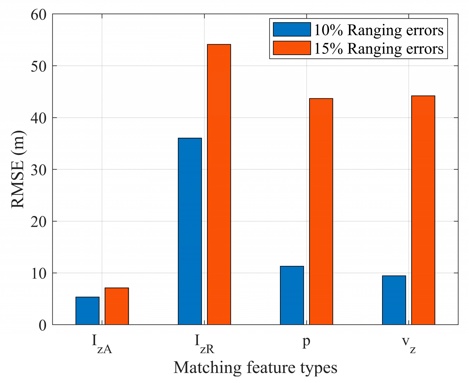
The RMSE of different matching features under different ranging errors is shown in Figure 5.

According to the simulation experiment results, the depth estimation performance of different matching features varies significantly under different ranging error conditions. Notably, the vertical sound intensity flux feature maintains an estimated RMSE of less than 10 m under 10% and 15% ranging error conditions. In contrast, the RMSE of other features, such as sound pressure, vertical particle velocity, and their combinations, is significantly higher than that of the vertical sound intensity flux. As the ranging error increases, their estimation accuracy decreases significantly. Furthermore, at modal nodes, the depth estimation of the vertical sound intensity flux feature exhibits minimal fluctuations, while other features show strong fluctuations. This indicates that the vertical sound intensity flux feature better reflects underwater depth information in depth estimation tasks and demonstrates strong robustness and resistance to ranging errors.

The Impact of Different SNR on Depth Estimation

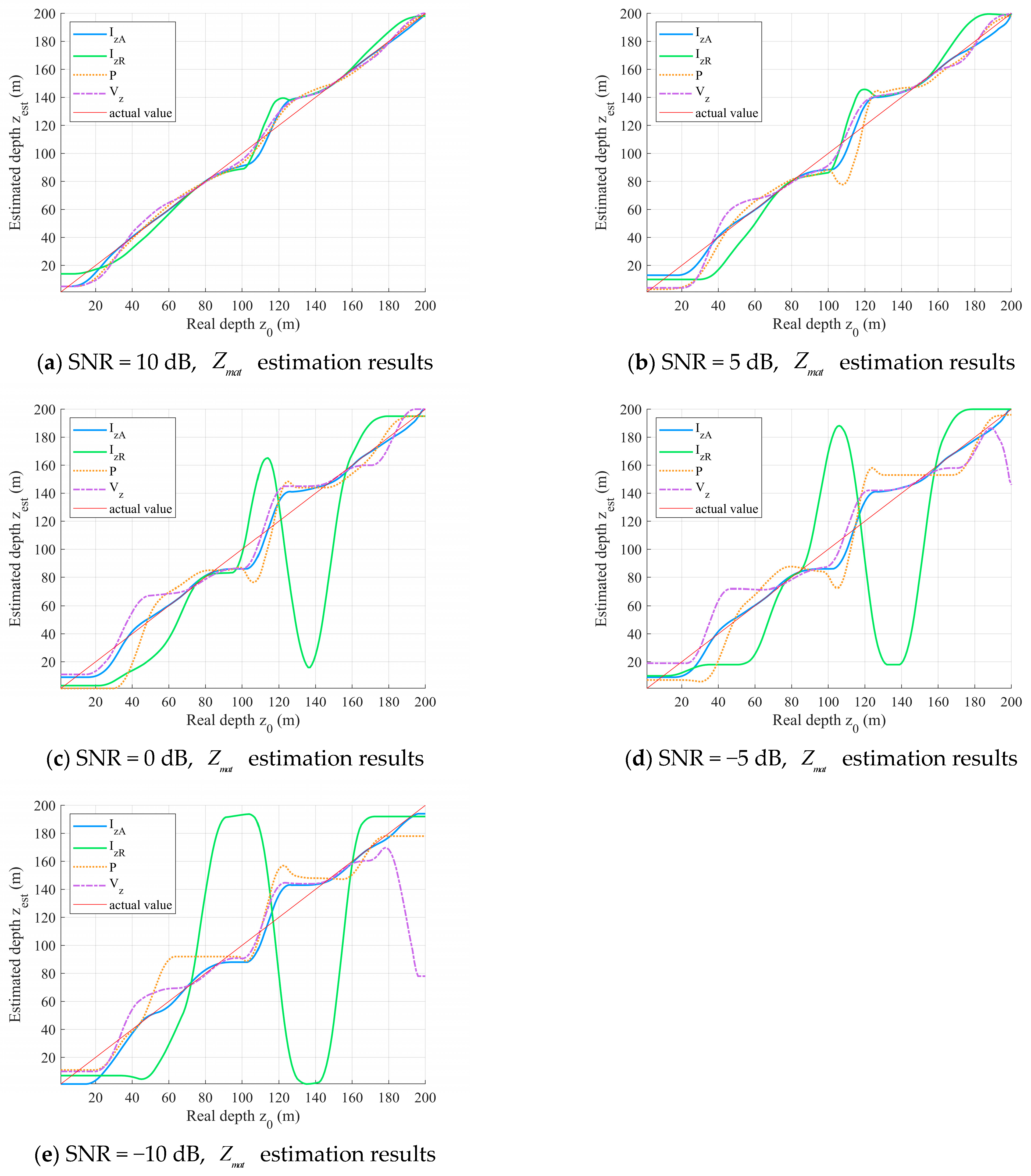
Assuming the target radiation noise is a continuous spectrum superimposed on a single-frequency line spectrum, simulation analysis was performed using four characteristics as matching quantities at SNR of −10 dB, −5 dB, 0 dB, 5 dB, and 10 dB. The specific results are shown in Figure 6.

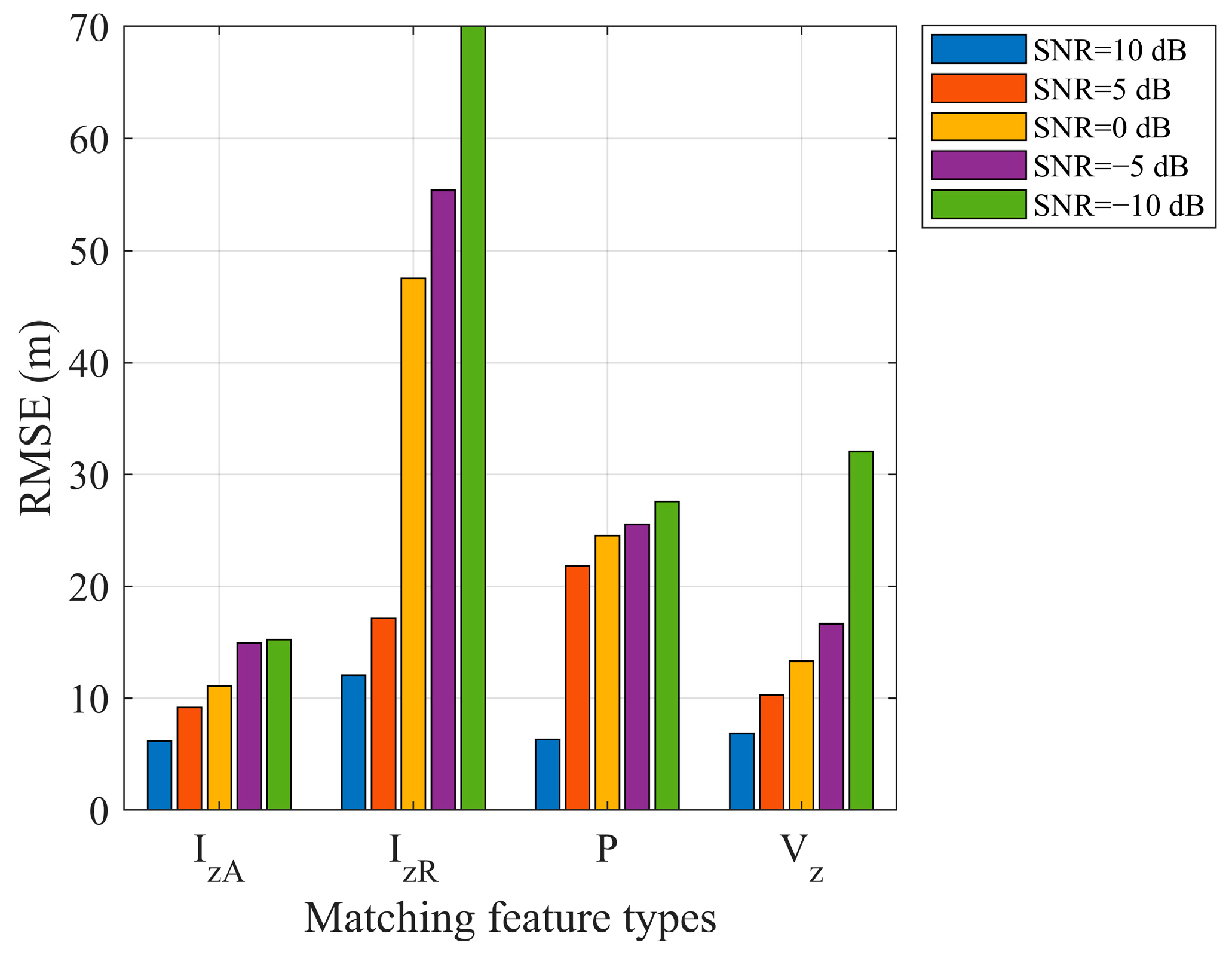
The RMSE of different matching features under different SNRs is shown in Figure 7.

According to the simulation results, it can be observed that under conditions with a high SNR, the performance differences among various matching features in depth estimation tasks are relatively small, with overall errors of approximately 10 m. However, as the SNR gradually decreases, the estimation accuracy of most matching features significantly deteriorates, exhibiting substantial deviations, and fails to meet the stability requirements for depth estimation in practical applications. In contrast, the estimation results using vertical sound intensity flux as the matching feature demonstrate excellent stability under various SNR conditions, with RMSE consistently maintained below 15 metres, highlighting its significant advantages in source depth estimation in complex underwater acoustic environments.

Impact of Sound Source Frequency Estimation Error on Depth Estimation

Since the matching field algorithm is highly dependent on the spatial structural characteristics of the sound field, the frequency of the sound source, as an important parameter affecting the sound propagation pattern, must be used as a known prior input model; otherwise, it will seriously affect the matching accuracy. For the frequency estimation of unknown underwater sound sources, errors are inevitable. This section analyses the depth estimation performance of different features under different sound source estimation errors. The specific results are shown in Figure 8.

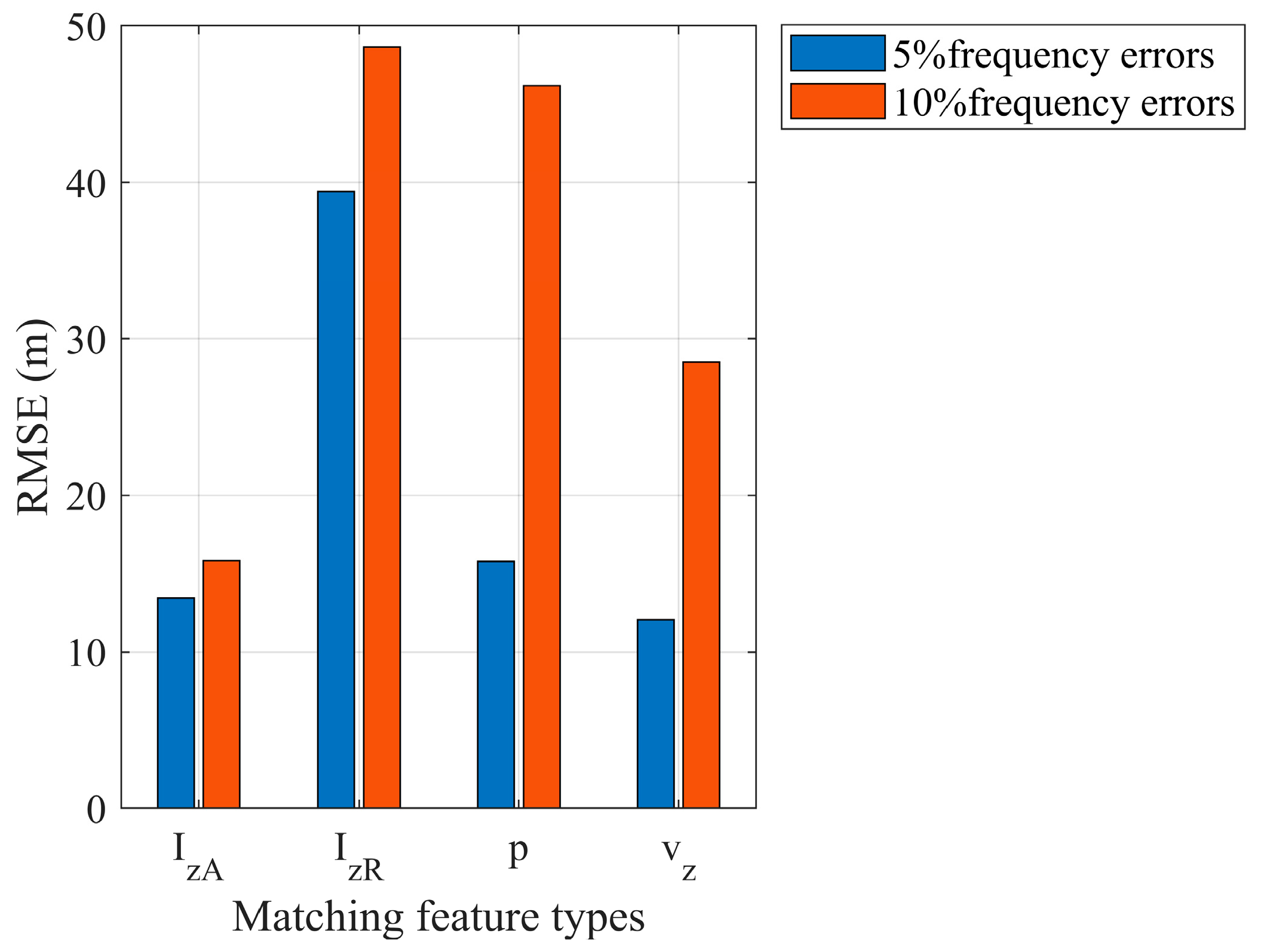
Under the same frequency estimation error, the RMSE of different matching features is shown in Figure 9.

According to the simulation results, all types of matching features exhibit significant performance degradation when frequency errors are present. Even a deviation of just a few Hz can cause significant shifts in the estimated source depth for some features, indicating that depth matching results are highly sensitive to frequency modelling. In contrast, although the RMSE of the vertical sound intensity stream feature is approximately 15 m when frequency errors are present, its error fluctuates relatively little under different frequency deviation conditions. Therefore, as a vector acoustic feature, the vertical sound intensity flux exhibits a certain degree of resistance to frequency modelling uncertainties and is suitable for complex or poorly defined acoustic localisation tasks.

This section validates the robustness and adaptability of the vertical sound intensity flow feature in underwater source depth estimation tasks through simulation analyses of different matching features under various disturbance conditions (range measurement errors, SNR variations, and frequency errors). Experimental results show: under ranging error perturbations, the RMSE of the vertical sound intensity stream feature remains within 10 m under 10% and 15% error conditions, significantly outperforming traditional features such as sound pressure, vertical velocity, and their combinations; in low SNR environments, the vertical sound intensity stream matching maintains relatively low error fluctuations (RMSE ≤ 15 metres), whereas other feature estimation results exhibit significant fluctuations and poor stability; Under frequency deviation, although all features are highly sensitive to frequency errors, the estimation results of vertical acoustic intensity flow exhibit relatively stable changes, demonstrating a certain degree of resistance to frequency modelling errors. These results fully highlight the adaptive advantages of vertical acoustic intensity flow features in complex environments, making them a deep estimation matching feature that combines both stability and precision.

2.3. Underwater Sound Source Depth Identification Based on Deep Learning and Vector Acoustic Features

Based on the above analysis, although the matching field algorithm exhibits excellent depth estimation performance under ideal conditions, it still faces several challenges in practical applications. Simulation experiments indicate that when the sound source is located near a modal node, the distribution of various acoustic field features becomes weak, exhibiting a minimum state, leading to significant fluctuations or a sharp increase in errors in the depth estimation results of the matching field algorithm in this region. This phenomenon stems from the node characteristics under the normalised wave theory, making traditional matching methods that rely on similarity metrics unable to accurately extract effective depth criteria in regions with weak interference. Additionally, traditional matching field algorithms generally rely on prior information such as the sound source frequency. When the actual frequency deviates or cannot be accurately obtained, model errors accumulate rapidly, leading to unstable or even completely ineffective estimation results, further limiting the applicability of this method in complex or unknown environments. To address these issues, this paper further introduces deep learning methods, constructing an end-to-end learning model to perform non-linear modelling of hidden features in complex interference structures. Specifically, considering that the vertical intensity flow exhibits stronger directionality and stability in characterising the vertical position of the sound source, this paper selects the vertical intensity flow as the network input feature, leveraging its stability under different frequencies and environmental errors to enhance the model’s perception capability of the modal node region. Compared to traditional physics-based matching algorithms, deep neural networks can learn complex feature representations under complex interference patterns through large-scale sample learning, demonstrating stronger generalisation and interference resistance capabilities. Next, this paper will provide a detailed introduction to the proposed source depth estimation model based on the ResNet-BiLSTM fusion structure (PB-RBLNet: Parallel BiLSTM and ResNet-based Branch Learning Network) and evaluate and analyse its performance under ranging errors and frequency errors.

2.3.1. Overall Framework

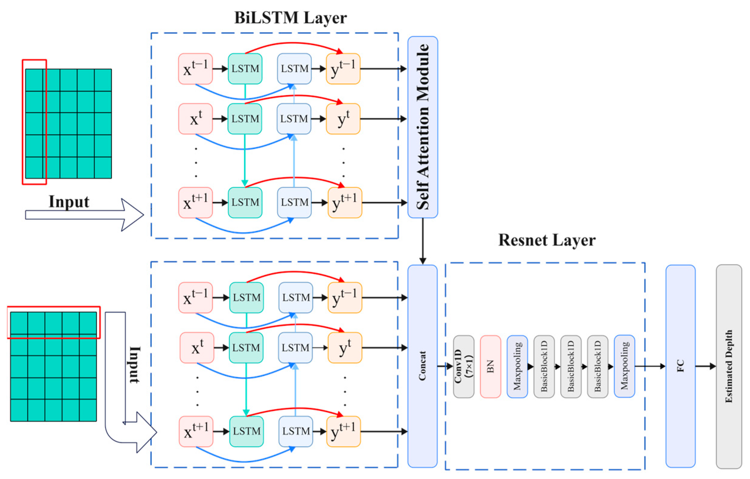
The model structure in this paper adopts a parallel dual-branch design: one BiLSTM network extracts deep-related features from the sound field sequence, while the other BiLSTM captures distance-related information. To extract deeper global depth information and address the issue of small feature values and weak feature representation capabilities at modal nodes, this model incorporates an attention mechanism, which is further concatenated with the original features and fed into the ResNet network. The ResNet module further extracts local features from the fused features, aiding in capturing more complex spatial variation patterns within the interference structure. Additionally, the residual connection structure of ResNet alleviates the vanishing gradient problem in deep network training, improving model training efficiency and generalisation capability. The final source depth prediction value is output through a fully connected layer. The overall block diagram is shown in Figure 10, and the detailed parameters are provided in

Table 2. PB-RBLNet Network Parameter Table.

Layer	Type	Input Shape	Output Shap
Input (vertical branch)		(1, 200, 1500)
BiLSTM1 (bidirectional, H = 128)	BiLSTM	(1, 200, 1500)	(1, 200, 256)
Self-attention module	Attention	(1, 200, 256)	(1, 256)
Input (horizontal branch)		(1, 1500, 200)
BiLSTM2 (bidirectional, H = 128)	BiLSTM	(1, 1500, 200)	(1, 1500, 256)
AvgPool	AvgPool1D	(1, 1500, 256)	(1, 256)
feature fusion	Concatenation	(1, 256) + (1, 256)	(1, 512)
ResNet module	Multi-layer residual blocks	(1 × 512)	(1 × 512)
Fully connected layer 1 (ReLU)	FC + ReLU	(1 × 512)	(1 × 256)
Fully connected layer 2	FC2	(1 × 256)	1 × 1 (output)

.

2.3.2. Network Model Structure Design

To estimate the depth of underwater sound sources, this paper proposes a neural network architecture that combines bidirectional temporal modelling with deep convolutional feature extraction. The overall structure of the network includes: a dual-branch BiLSTM module, a Scaled Dot-Product Attention module, a feature fusion layer, a ResNet1D module, and a fully connected regression layer. The model structure is shown in Section 2.3.1, and the functions of each module in the network are described below.

The model input is a two-dimensional matrix of size 200 × 1500, where 200 represents the number of depth points, and 1500 represents the acoustic features on the distance vector corresponding to each depth point. Each sample is a two-dimensional matrix, and the model processes one sample at a time, with a total of 50 groups and 10,000 data points. To simultaneously model the trends of sound field changes in both the distance and depth directions, the network is designed with two independent BiLSTM branches. Horizontal BiLSTM: Each row is treated as a sequence input, processing a total of 200 sequences. The vertical BiLSTM: each column is treated as a sequence input, processing a total of 1500 sequences. The attention mechanism module further introduces the Scaled Dot-Product Attention mechanism to achieve feature-weighted aggregation based on the output of the vertical BiLSTM. Let $Q$, $K$ and $V$ represent the query matrix, key matrix, and value matrix, respectively. The attention output vector is:

$$Attention(Q,K,V)=\mathit{Soft}\max ({\displaystyle \frac{Q{K}^T}{\sqrt{d_k}}})V$$

(17)

In the above equation, $\sqrt{d_k}$ is the feature dimension. Since Attention has already performed feature-weighted aggregation, no additional pooling operations are required. The result is a weighted sum that reflects the importance of each depth position. The output vectors from both directions are concatenated to form a 512-length fused feature input for the ResNet1D module. To further learn the higher-order nonlinear expressions of the fused features, a ResNet module based on 1D convolution is designed, consisting of multiple residual blocks. Each residual block includes: Conv1D, BatchNorm, ReLU activation function, and residual connection; All residual blocks maintain the same number of input and output channels (512), ensuring that the feature dimension remains unchanged during residual propagation. Regression prediction layer: The 512-dimensional feature vector output by the ResNet1D module is mapped to the final deep regression output through two fully connected layers: Fully connected layer 1: 512 → 256, with the ReLU activation function; Fully connected layer 2: 256 → 1, outputting the deep estimation value of the sound source.

2.3.3. Evaluation Criteria

This paper uses the following indicators to comprehensively evaluate the performance of the model: accuracy within a certain threshold (Precision within ± X m, PAE) and root mean square error (RMSE). These indicators are defined as follows:

$$RMSE=\sqrt{{\displaystyle \frac{1}{N}}{{\displaystyle \sum _{i=1}^N({\widehat{y}}_i-y_i)}}^2}$$

(18)

RMSE can effectively measure the average deviation between model predictions and actual values, but this metric is sensitive to outliers and can be significantly affected by a few extreme error samples, limiting its ability to reflect overall estimation performance. To further evaluate the practicality and robustness of the model in actual engineering applications, this paper introduces depth prediction accuracy (DPA) as a supplementary evaluation metric. DPA represents the proportion of samples whose prediction errors fall within a given error threshold, providing an intuitive reflection of the model’s applicability under different precision requirements. Compared to RMSE, DPA aligns more closely with the ‘usability’ standards in engineering applications, aiding in a comprehensive evaluation of the model’s actual performance in complex acoustic environments from multiple dimensions. Therefore, the combined analysis of RMSE and DPA can more comprehensively reflect the model’s depth estimation capability and stability under different SNR and ranging error conditions.

$$DP{A}_{xm}={\displaystyle \frac{1}{N}}{\displaystyle \sum _{i=1}^N\partial (\left|{\widehat{y}}_i-y_i\right|<x)}$$

(19)

where $\partial (·)$ is an indicator function.

3. Experimental Results and Discussion

To comprehensively evaluate the source depth estimation performance of the proposed model in complex marine environments, this paper constructs a simulation dataset based on the marine acoustic field parameters shown in Table 1. using normalised wave theory. The source depth range is set from 1 to 200, and the training set covers an SNR range from −15 dB to 15 dB. To simulate the acoustic field characteristics under various underwater acoustic channels and test the model’s stability and generalisation capability, three typical non-ideal error conditions are introduced in the test set: (1) ±10% and ±15% ranging errors; (2) frequency shifts within the range of −5 Hz to +5 Hz; (3) SNR perturbations within the same range (−15 dB to 15 dB). The training set and test set are in an 8:1 ratio, ensuring that the test set is representative while retaining sufficient samples for model training.

3.1. Performance Analysis Under Different SNR

In this section, under a ±10% ranging error condition, the system compares the depth estimation performance of the proposed PB-RBLNet model at different SNRs and compares it with the RMSE of ResNet, LSTM, and traditional matching field algorithms. The specific results are shown in Figure 11 and

Table 3. DPA_5m for different algorithms.

SNR (dB)	PB-RBLNet	ResNet	LSTM	MFP
15	96.32%	95.44%	88.12%	84.10%
10	92.96%	89.75%	84.23%	78.76%
5	88.17%	70.59%	53.14%	51.98%
0	70.22%	32.21%	42.17%	42.28%
−5	49.53%	26.13%	38.53%	36.51%
−10	38.39%	18.89%	30.94%	28.49%
−15	35.51%	12.14%	9.68%	8.4%

:

By comparing the RMSE curves of the four different algorithms under different SNRs, it can be observed that: under higher SNR conditions, all algorithms can achieve relatively accurate depth estimation, with RMSE generally maintained within 5 m or even lower, demonstrating stable overall performance. However, as the SNR decreases, the estimation accuracy of all algorithms exhibits varying degrees of fluctuation. Among them, the Matching Field Processor (MFP) and LSTM models are particularly sensitive to changes in the SNR, with the RMSE rising to approximately 10 m at 0 dB, resulting in a significant decline in accuracy. In contrast, the ResNet model performs similarly to the proposed PB-RBLNet model in the SNR range below 0 dB. However, under lower SNR conditions, the RMSE of all algorithms except the PB-RBLNet model exceeds 15 m, failing to meet the accuracy requirements of practical engineering applications. Further observation of the stability of each algorithm under different ranging error conditions reveals that the PB-RBLNet model exhibits smaller error fluctuations at all SNR levels, especially in the low SNR range, where its estimation accuracy decline trend is more stable, demonstrating excellent stability. As shown in Table 3, under high SNR conditions (15 dB), the PB-RBLNet model performs exceptionally well, achieving an effectiveness of 96.32%, significantly outperforming traditional methods, indicating that the integration of deep learning architectures can more effectively capture and utilise the multi-dimensional feature information of signals. As the SNR decreases to medium-low levels (5 dB and below), performance differences among the models gradually become apparent. The PB-RBLNet model demonstrates strong stability, maintaining an effectiveness of 35.51% even in an extremely low SNR environment of −15 dB, far exceeding ResNet (12.14%), LSTM (9.68%), and traditional MFP (8.40%). This indicates that the PB-RBLNet model, combining convolutional neural networks and bidirectional long short-term memory networks, can still stably extract effective features even under severe noise interference. Additionally, the overall performance of the traditional MFP method is relatively low, with accuracy significantly decreasing under high-noise conditions, reflecting its sensitivity to changes in environmental parameters and noise. Overall, the PB-RBLNet model outperforms other comparison algorithms in terms of noise resistance and ranging error adaptability, with more stable depth estimation performance and higher engineering application potential.

3.2. Performance Analysis Under Different Ranging Errors

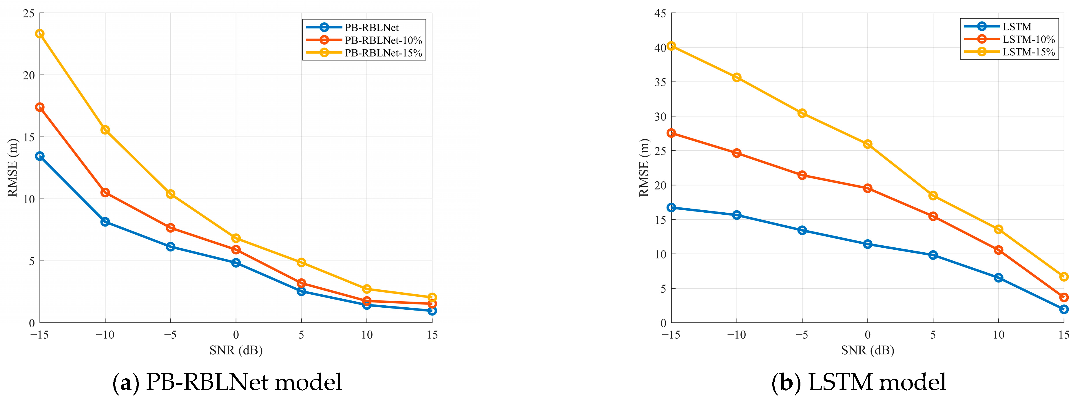
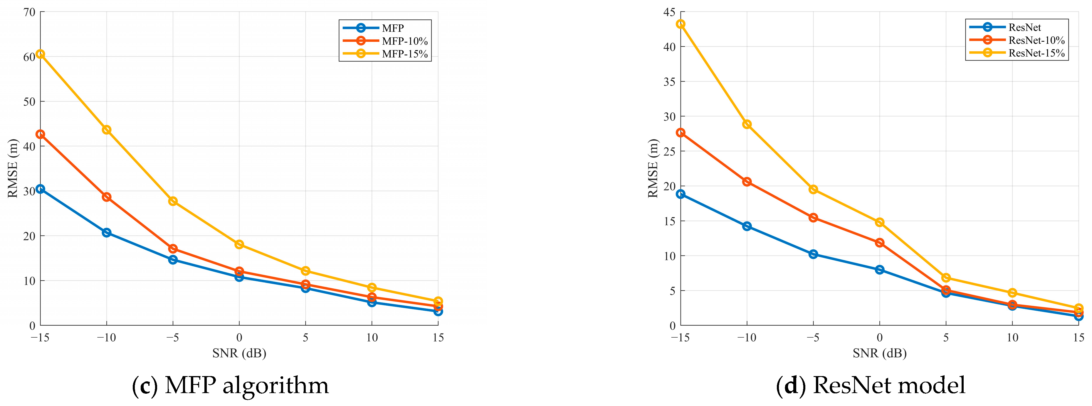
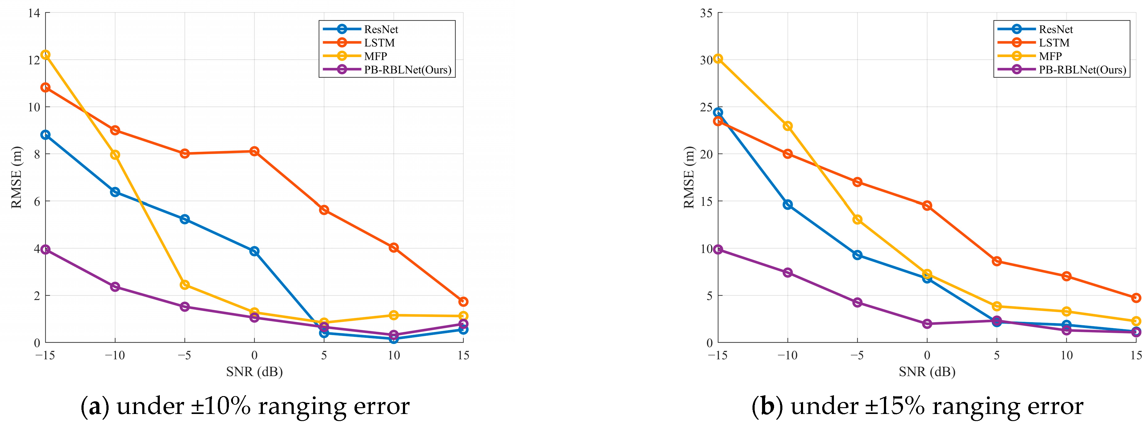
To evaluate the performance of different algorithms under varying error conditions, this section compares the depth estimation performance of different models at different SNR levels under ±10% and ±15% ranging error scenarios. The analysis is based on the differences in RMSE caused by ranging error changes to quantify the stability and interference resistance of each model to ranging error interference. The experimental results of different models under different ranging errors are shown in Figure 12 and Figure 13:

By comparing the RMSE curves of different models and algorithms under various SNR conditions with different ranging errors, it can be observed that the PB-RBLNet model demonstrates superior estimation accuracy in high-SNR regions (SNR > 0 dB), with its RMSE consistently maintained at a low level. As the SNR decreases, although the RMSE values of all models show an increasing trend, the error growth rate of the proposed PB-RBLNet model is significantly lower, with the overall RMSE consistently controlled within 15 m, while the remaining models exceed this threshold. Additionally, the RMSE difference plot further validates that the proposed model exhibits the lowest RMSE fluctuation range under different ranging error conditions, demonstrating excellent error stability and consistency. Finally, the comparison table of $DP{A}_{5m}$ under different ranging errors shows that the PB-RBLNet model has a higher probability than the other models under different ranging errors, as detailed in

Table 4. DPA_5m Comparison table under different ranging errors.

	$\left|\frac{\Delta \mathbf{r}}{\mathbf{r}}\right|<10\mathbf{\%}$				$\left|\frac{\Delta \mathbf{r}}{\mathbf{r}}\right|<15\mathbf{\%}$
SNR (dB)	PB-RBLNet	ResNet	LSTM	MFP	PB-RBLNet	ResNet	LSTM	MFP
15	96.32%	95.44%	88.12%	84.10%	94.47%	93.97%	68.69%	61.47%
10	92.96%	89.75%	84.23%	78.76%	92.17%	84.36%	58.18%	46.84%
5	88.17%	70.59%	53.14%	51.98%	86.55%	66.18%	20.91%	32.41%
0	70.22%	32.21%	42.17%	42.28%	61.31%	30.87%	13.54%	21.64%
−5	49.53%	26.13%	38.53%	36.51%	41.34%	20.11%	11.42%	11.77%
−10	38.39%	18.89%	30.94%	28.49%	27.63%	17.45%	8.34%	6.23%
−15	35.51%	12.14%	9.68%	8.4%	17.51%	8.17%	6.75%	4.25%

. As shown above, the proposed structure demonstrates strong interference resistance when faced with ranging error disturbances, effectively enhancing the reliability and effectiveness of sound source depth estimation.

3.3. Performance Analysis Under Different Frequency Errors

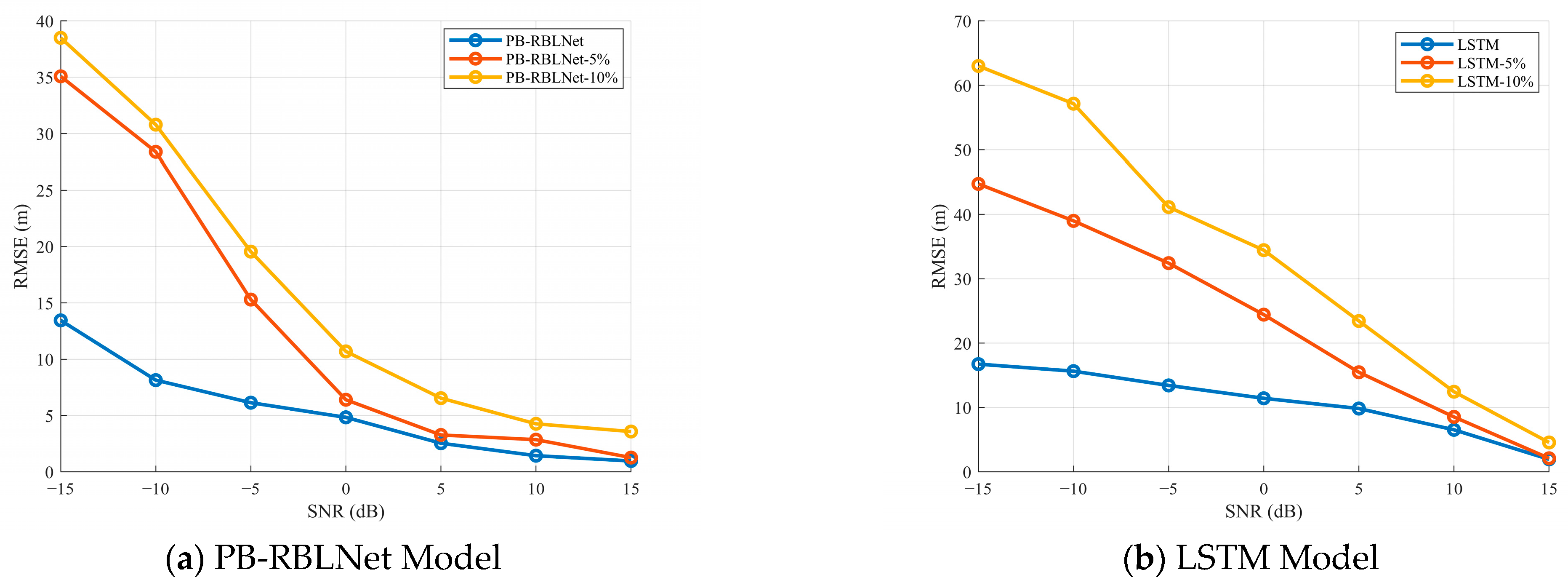
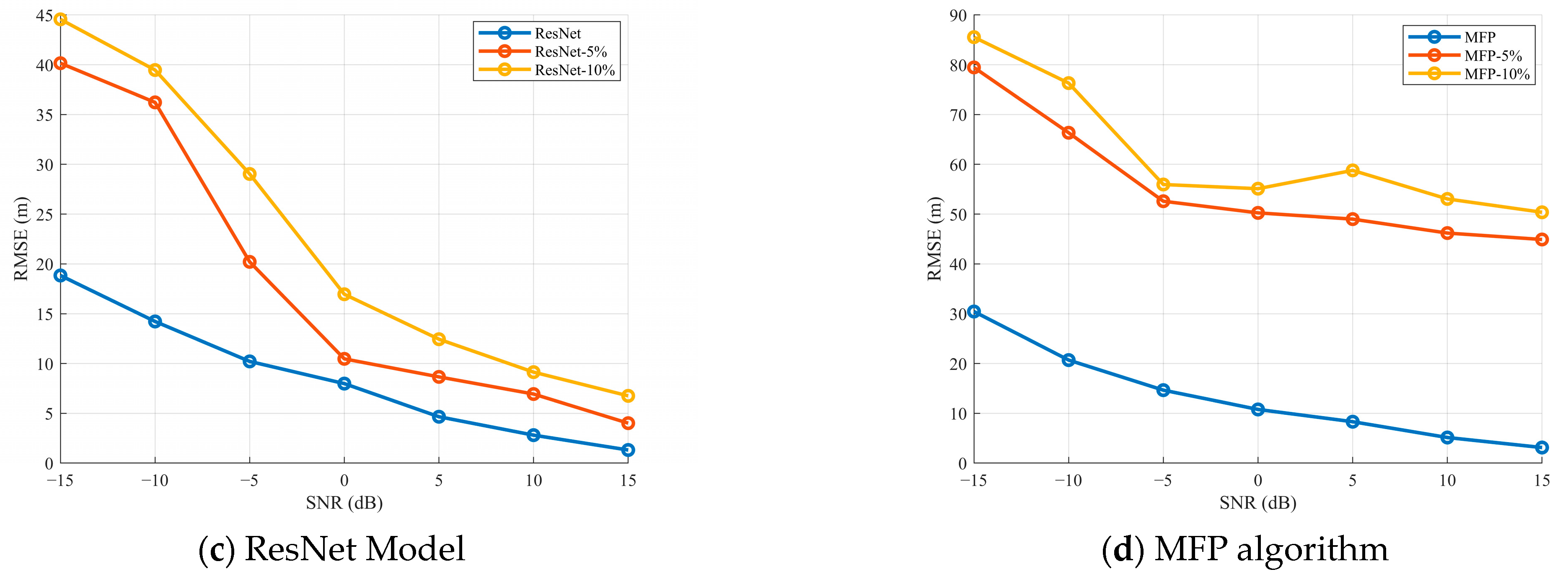
In this section, the proposed PB-RBLNet model is compared with other models in terms of depth estimation performance under different SNR conditions, with frequency estimation errors of 5% and 10%. The specific experimental results are as follows:

As shown in Figure 14 and Figure 15, under high SNR conditions, despite the presence of frequency errors, the depth estimation accuracy of the deep learning algorithm is significantly superior to that of the matching field algorithm, exhibiting a lower RMSE. However, under low SNR conditions, the estimation accuracy decreases significantly, and the impact of frequency errors on model performance becomes markedly more pronounced. This phenomenon stems from the fact that the interference fringe structure in the sound field is highly sensitive to frequency. Interference fringes are formed by the superposition of multiple modes, and their spatial distribution shifts noticeably with even minor changes in frequency, leading to changes in the received features. Under high SNR conditions, despite slight shifts in features, the model may still capture their overall structure; however, under low SNR conditions, the interference structure is overwhelmed by noise, and the accumulation of frequency errors causes a severe mismatch between the signal and the template, significantly weakening the model’s discriminative capability. In contrast, the PB-RBLNet model proposed in this paper can still keep the RMSE within 5 m when the SNR is above 0 dB and demonstrates greater stability and robustness under different frequency error conditions.

3.4. Computational Complexity Analysis

The proposed PB-RBLNet model is relatively complex, as it integrates parallel BiLSTM layers with a ResNet1D module, introducing additional parameters compared to standalone LSTM or ResNet architectures. The theoretical computational cost can be evaluated in terms of floating-point operations (FLOPs) and the number of parameters. Specifically, for a BiLSTM layer with $h$ hidden units and input feature dimension $d$ over a sequence length of $T$, the approximate FLOPs are $O(4\cdot h\cdot (h+d)\cdot T)$. The ResNet1D module adds convolutional operations, resulting in a moderate increase in total FLOPs. Despite the increased complexity, the model maintains practical inference speed.

The input shape of PB-RBLNet is (batch_size, sequence_length, feature_dim) = (1, 200, 1500), where sequence_length = 200 represents vertical depth points, and feature_dim = 1500 corresponds to horizontal distance samples. The BiLSTM hidden units are set to 256, and ResNet1D has 4 convolutional layers with 256 output channels each. The detailed parameter counts and FLOPs for PB-RBLNet and benchmark models are summarized in

Table 5. Parameter counts and FLOPs for PB-RBLNet and benchmark models.

Model	Parameters	FLOPs
PB-RBLNet	3,650,896	1.34 G
LSTM	1,798,912	719 M
ResNet1D	1,742,848	697 M

.

On a standard GPU, the average prediction time per sample is in the millisecond range, demonstrating its feasibility for near real-time processing. Compared with benchmark methods, PB-RBLNet requires more computations than a single LSTM due to its deeper architecture, but it achieves significantly improved estimation accuracy and robustness. Compared to ResNet1D, the parallel BiLSTM branch enhances temporal modeling capability while maintaining moderate computational cost. Although MFP (matched-field processing) has fewer parameters, it requires extensive correlation calculations at runtime, resulting in high computational overhead; once PB-RBLNet is trained, its inference is much faster, avoiding the online computational burden of MFP. Overall, considering the substantial gains in RMSE and robustness, the additional computational cost of PB-RBLNet is acceptable, making it practical for real-world applications, especially those requiring near real-time operation.

3.5. Discussion

PB-RBLNet mitigates the modal node problem by using active acoustic intensity as its input feature, which preserves stable depth-sensitive information even when the source is located near a modal node. Active intensity represents the net energy flow rather than locally stored reactive energy; therefore, even when the individual amplitudes of pressure p or particle velocity v approach zero near a node, the coherent relationship between p and v still forms a non-zero, directionally meaningful energy-flow feature. The vertical component of active intensity further suppresses phase-only noise caused by phase fluctuations, improving the effective SNR in the nodal region. This provides PB-RBLNet with a robust, non-degenerate input representation, significantly alleviating the feature-vanishing issue associated with modal nodes.

Within the network, the ResNet1D branch extracts higher-order local structures through stacked convolutions and residual connections, effectively learning local filters analogous to first- and second-order derivatives. Even when feature amplitudes are near zero at modal nodes, spatial variations such as slope, curvature, or inflection remain non-zero and identifiable. Unlike traditional MFP, which relies on point-to-point amplitude matching and cannot exploit weak but distributed patterns, ResNet1D captures these higher-order variations, recovering meaningful structural information from regions with near-zero absolute feature values. Meanwhile, the BiLSTM branch leverages bidirectional contextual modeling and gated information flow to integrate neighboring high-energy regions, reinforcing weak signals at modal nodes. This neighborhood-based enhancement is unattainable for traditional MFP, which lacks mechanisms for cross-sample contextual integration.

The fusion of ResNet1D and BiLSTM generates a feature space that is simultaneously noise-resistant, sensitive to weak patterns, and spatially consistent, enabling PB-RBLNet to maintain smooth and stable depth estimation performance even near modal nodes. Compared with traditional scalar acoustic features such as sound pressure or single-component particle velocity, vertical acoustic intensity flow inherently provides a more stable and robust representation of the underwater acoustic field. Physically, it integrates both pressure and velocity components to describe the net energy flux, effectively reflecting the vertical interference structure. Derived from the real part of the complex sound intensity, it suppresses phase ambiguities and random noise fluctuations, improving robustness against environmental variations, measurement noise, and frequency deviations.

Moreover, the stability of vertical acoustic intensity flow stems from its energy-based nature—it reflects net acoustic power flow rather than instantaneous oscillations. Consequently, even under low SNR conditions or slight deviations in source–receiver geometry, the vertical acoustic intensity flow maintains a consistent interference pattern closely related to source depth, making it particularly suitable for depth estimation in complex and uncertain ocean environments. The proposed deep learning framework further demonstrates clear advantages over traditional MFP. While MFP relies heavily on accurate environmental modeling and is highly sensitive to sound speed profile or bathymetry mismatches, PB-RBLNet can directly learn nonlinear mappings from vertical acoustic intensity flow patterns to source depth, effectively compensating for modeling uncertainties. By combining vertical acoustic intensity flow features with PB-RBLNet, the model captures both temporal dependencies and local spatial correlations, achieving superior estimation accuracy, faster inference, and better generalization under variable environmental conditions compared with MFP-based approaches.

Nevertheless, the method has several limitations. It relies on vertical particle velocity measurements, requiring vector hydrophones, which are more expensive and complex to deploy than conventional scalar sensors. Multi-depth and multi-range data acquisition is experimentally challenging. PB-RBLNet, while improving depth estimation accuracy, also increases computational and memory demands, potentially limiting real-time deployment on resource-constrained platforms. Although the method shows robustness to distance and frequency errors, its performance may degrade in highly dynamic or strongly range-dependent ocean environments, particularly at low SNR, unless additional environmental adaptation is applied. Furthermore, deep learning models require extensive and diverse training datasets, and collecting such data in real ocean settings entails considerable cost and effort.

4. Conclusions

This paper addresses the issue of low utilisation of underwater acoustic field information by fully leveraging the advantage of vector hydrophones, which can simultaneously collect sound pressure and velocity data. It selects vertical sound intensity flux as a key feature and verifies its effectiveness in depth estimation compared to other acoustic features. Based on this, the PB-RBLNet structure, combining parallel dual-layer BiLSTM and ResNet (PB-RBLNet), is proposed. This model can jointly explore the coupling relationship between depth and distance, effectively improving estimation performance. Through extensive simulation experiments, this paper systematically evaluates the depth estimation accuracy of the PB-RBLNet model under different SNR conditions and further examines its stability under ranging errors and frequency errors. The results show that when the SNR is above 0 dB, PB-RBLNet can stably control the RMSE within 5 m, and it still demonstrates superior stability under distance and frequency disturbances. In low SNR environments, the model also maintains better interference resistance compared to other comparison methods. However, it should be noted that at low SNR, PB-RBLNet remains sensitive to frequency errors, which provides a research direction for future improvements in algorithm robustness.

References

1. Yuan, X.; Guo, L.; Luo, C.; Zhou, X.; Yu, C. A Survey of Target Detection and Recognition Methods in Underwater Turbid Areas. Appl. Sci. 2022, 12, 4898. [Google Scholar] [CrossRef]
2. Li, H.; Yang, K.; Duan, R.; Lei, Z. Joint Estimation of Source Range and Depth Using a Bottom-Deployed Vertical Line Array in Deep Water. Sensors 2017, 17, 1315. [Google Scholar] [CrossRef] [PubMed]
3. Kniffin, G.P.; Boyle, J.K.; Zurk, L.M.; Siderius, M. Performance metrics for depth-based signal separation using deep vertical line arrays. J. Acoust. Soc. Am. 2016, 139, 418–425. [Google Scholar] [CrossRef] [PubMed]
4. McCargar, R.; Zurk, L.M. Depth-based signal separation with vertical line arrays in the deep ocean. J. Acoust. Soc. Am. 2013, 133, EL320–EL325. [Google Scholar] [CrossRef] [PubMed]
5. Byun, G.; Song, H.C.; Kim, J.S. Performance comparisons of array invariant and matched field processing using broadband ship noise and a tilted vertical array. J. Acoust. Soc. Am. 2018, 144, 3067–3074. [Google Scholar] [CrossRef] [PubMed]
6. Santos, P.; Felisberto, P.; Jesus, S.M. Vector Sensor Arrays in Underwater Acoustic Applications. In Emerging Trends in Technological Innovation; Camarinha-Matos, L.M., Pereira, P., Ribeiro, L., Eds.; DoCEIS 2010. IFIP Advances in Information and Communication Technology; Springer: Berlin/Heidelberg, Germany, 2010; Volume 314. [Google Scholar] [CrossRef]
7. Rong, L.; Lei, B.; Gu, T.; He, Z. Depth Estimation of an Underwater Moving Source Based on the Acoustic Interference Pattern Stream. Electronics 2025, 14, 2228. [Google Scholar] [CrossRef]
8. Yu, Y.; Ling, Q.; Xu, J. Pressure and velocity cross-spectrum of normal modes in low-frequency acoustic vector field of shallow water and its application. J. Syst. Eng. Electron. 2015, 26, 241–249. [Google Scholar] [CrossRef]
9. Yang, G.; Yin, J.; Yu, Y.; Shi, Z. Depth classification of underwater targets based on complex acoustic intensity of normal modes. J. Ocean Univ. China 2016, 15, 241–246. [Google Scholar] [CrossRef]
10. Zhao, A.; Bi, X.; Hui, J.; Zeng, C.; Ma, L. Application and Extension of Vertical Intensity Lower-Mode in Methods for Target Depth-Resolution with a Single-Vector Sensor. Sensors 2018, 18, 2073. [Google Scholar] [CrossRef] [PubMed]
11. Lu, Y.; Yuan, Y.; Liu, M.; Wei, Y.; Tu, X.; Qu, F. An Underwater Wideband Sound Source Localization Method Based on Light Neural Network Structure. IEEE Sens. J. 2024, 24, 20970–20980. [Google Scholar] [CrossRef]
12. Wang, W.; Wang, Z.; Su, L.; Hu, T.; Ren, Q.; Gerstoft, P.; Ma, L. Source depth estimation using spectral transformations and convolutional neural network in a deep-sea environment. J. Acoust. Soc. Am. 2020, 148, 3633–3644. [Google Scholar] [CrossRef] [PubMed]
13. Weiss, A.; Arikan, T.; Wornell, G.W. Direct Localization in Underwater Acoustics Via Convolutional Neural Networks: A Data-Driven Approach. In Proceedings of the 2022 IEEE 32nd International Workshop on Machine Learning for Signal Processing (MLSP), Xi’an, China, 22–25 August 2022; pp. 1–6. [Google Scholar]
14. Liang, Y.; Chen, Y.; Meng, Z.; Zhou, X.; Zhang, Y. A Deep-Sea Broadband Sound Source Depth Estimation Method Based on the Interference Structure of the Compensated Beam Output. J. Mar. Sci. Eng. 2023, 11, 2059. [Google Scholar] [CrossRef]
15. Bi, X.; Hui, J.; Zhao, A.; Wang, B.; Ma, L.; Li, X. Underwater Target Depth Classification Method Based on Vertical Acoustic Intensity Flux. J. Electron. Inf. Technol. 2021, 43, 3237–3246. [Google Scholar] [CrossRef]
16. Bi, X.; Hui, J.; Zhao, A.; Wang, B.; Ma, L.; Li, X. Research on Acoustic Target Depth Classification Method Based on Matching Field Processing in Shallow Water. J. Electron. Inf. Technol. 2022, 44, 3917–3930. [Google Scholar] [CrossRef]
17. Gur, B. Particle velocity gradient based acoustic mode beamforming for short linear vector sensor arrays. J. Acoust. Soc. Am. 2014, 135, 3463–3473. [Google Scholar] [CrossRef] [PubMed]
18. Chapman, D.M.F.; Thomson, D.J.; Ellis, D.D. Modeling air-to-water sound transmission using standard numerical codes of underwater acoustics. J. Acoust. Soc. Am. 1992, 91, 1904–1910. [Google Scholar] [CrossRef]
19. Dall’osto, D.R.; Dahl, P.H.; Choi, J.W. Properties of the acoustic intensity vector field in a shallow water waveguide. J. Acoust. Soc. Am. 2012, 131, 2023–2035. [Google Scholar] [CrossRef] [PubMed]
20. Jensen, F.B.; Kuperman, W.A.; Porter, M.B.; Schmidt, H.; Tolstoy, A. Computational Ocean Acoustics. Phys. Today 1994, 47, 91–92. [Google Scholar] [CrossRef]
21. Buckingham, M.J.; Giddens, E.M. On the acoustic field in a Pekeris waveguide with attenuation in the bottom half-space. J. Acoust. Soc. Am. 2006, 119, 123–142. [Google Scholar] [CrossRef] [PubMed]
Figure 1. Three-layer medium model.
Jmse 13 02284 g001
Figure 2. Projection diagram of vibration velocity v and its three orthogonal components v x , v y , and v z .
Jmse 13 02284 g002
Figure 3. Computational process for estimating the depth of underwater deep sources based on matching fields.
Jmse 13 02284 g003
Figure 4. Depth estimation results for different matching amounts under different ranging errors.
Jmse 13 02284 g004aJmse 13 02284 g004b
Figure 5. RMSE results for different matching features under various range errors.
Jmse 13 02284 g005
Figure 6. Deep estimation results for different matching features at different SNRs.
Jmse 13 02284 g006
Figure 7. RMSE results for different matching features under various SNR.
Jmse 13 02284 g007
Figure 8. Deep estimation results for different matching features under different frequency estimation errors.
Jmse 13 02284 g008
Figure 9. Depth estimation results for different matching features under different frequency estimation errors.
Jmse 13 02284 g009
Figure 10. Overall framework diagram of the model.
Jmse 13 02284 g010
Figure 11. RMSE curves of different algorithms under different SNRs.
Jmse 13 02284 g011
Figure 12. Comparison of RMSE between different models under different ranging errors.
Jmse 13 02284 g012aJmse 13 02284 g012b
Figure 13. RMSE difference curves for different models under different ranging errors.
Jmse 13 02284 g013
Figure 14. Comparison of RMSE for different models at different frequency errors.
Jmse 13 02284 g014aJmse 13 02284 g014b
Figure 15. RMSE difference curves for different models at different frequency errors.
Jmse 13 02284 g015