Article

Intelligent Diagnosis of Ship Propulsion Motor Bearings Based on Dynamic Class Weights

by
Guohua Yan
1,
Xiaoding Wang
1,
Kai Liu
2,
Jingran Kang
3 and
Xinhua Yi
1,*
1
Department of Mechanical and Automotive Engineering, NingBo University of Technology, Ningbo 315211, China
2
Navigation Technology Department, Tianjin Maritime College, Tianjin 300355, China
3
Geely Automobile Research Institute (Ningbo) Co., Ltd., Ningbo 315211, China
*
Author to whom correspondence should be addressed.
J. Mar. Sci. Eng. 2025, 13(11), 2204; https://doi.org/10.3390/jmse13112204
Submission received: 27 October 2025 / Revised: 14 November 2025 / Accepted: 16 November 2025 / Published: 19 November 2025

Abstract

As an important part of the ship’s power system, the bearing operation status of the propulsion motor is directly related to the reliability and safety of the whole system. However, in the field of marine propulsion motor bearing fault diagnosis, the data imbalance problem seriously affects the performance of the fault detection model. Due to the scarcity of fault data relative to normal operation data, traditional diagnostic methods are ineffective in dealing with unbalanced data. To solve this problem, a dynamic class weighting solution is proposed. The dynamic class weighting method introduces the weight coefficient λ on the basis of the traditional class weighting, which can adjust the class weight value in real time according to the training situation, and comprehensively considers the data distribution and the training situation to ensure that the model can learn better even in the case of insufficient data. Testing on the imbalanced distribution of bearing natural-failure data shows that the proposed method achieves a 5.25% improvement in diagnostic accuracy compared to direct training. Compared with traditional class-weighted approaches, diagnostic accuracy is enhanced by 3.56%, effectively mitigating the impact of scarce and unevenly distributed failure data on model training.

1. Introduction

Permanent magnet synchronous motors (PMSMs) are indispensable key devices in modern industry due to their high efficiency, high performance, compact design, and rapid response [1], and play a key role in the aerospace, marine, and automotive fields. As the core component of the modern ship power system, the ship permanent magnet propulsion motor bears the important task of energy conversion and transfer, provides reliable and efficient power for ships, and plays an important role in ship performance, economy and environmental protection. However, due to the special working environment of the ship and the complex and changeable navigational conditions, the propulsion motor works in an unfavourable environment with high temperatures, high humidity, salt spray corrosion, and overload, etc. The bearings are subject to friction and impact from the rotating body over a long period, which can easily damage them, leading to faults. Bearings are the most fault-prone components in motors, accounting for about 30–40% of motor failures [2]. Therefore, it is crucial to ensure the reliability and stability of motor bearings under harsh environmental conditions. There is an urgent need for academia and industry to enhance in-depth research and continuous advancement of fault analysis in this area in order to improve fault diagnosis techniques and methods, effectively address challenges and risks, and ensure the safe operation and sustained performance of ship propulsion systems.
Bearings are important components of electric motors, and researchers and scholars have been conducting extensive studies to improve their performance and reliability. Zhao et al. [3] used the EMD method to process the vibration signals of bearings, calculated the sample entropy of IMF components as fault characteristics, and then combined it with Back Propagation Neural Network (BPNN) to achieve fault identification, while optimising the key parameters in BPNN using a hybrid frog hopping algorithm. Mohammad-Alikhani et al. [4] proposed a generalised fault diagnosis method for deep residual networks with long and short term memory conditioning, which was evaluated using the motor turn-to-turn short circuit fault test and the Case Western Reserve University bearing fault dataset in the USA, and achieved an accuracy of 100 per cent on both datasets, which were different in terms of both fault types and signal types. Verstraete et al. [5] processed the vibration signals of bearings using STFT, CWT and Hilbert–Huang Transform (HHT), respectively, and generated the corresponding 2D images, which were then fed into a CNN architecture for classification and fault diagnosis, and explored the diagnostic effects of three time-frequency analysis methods. Ayas et al. [6] designed a deep residual CNN for bearing fault diagnosis, which transformed vibration signals into grayscale maps as inputs to the network, achieving diagnostic accuracy of 99.98%. Celtikoglu et al. [7] used a total of 18 commonly used time-frequency and frequency domain analysis methods to process the vibration signals of the bearings and generate the corresponding images, respectively, and then used the migration learning method based on the ResNet-99 network to identify the fault types, in order to explore a more suitable signal visualisation method for bearing fault diagnosis. Kim et al. [8] designed a one-dimensional dilated CNN using the original vibration signals of the bearings as inputs to the network, and the diagnostic accuracy reached 100% even in the presence of noise, and the diagnostic accuracy reached 99%. Guo et al. [9] designed a diagnostic method combining a CNN and BiLSTM, using the vibration signals of bearings as inputs to the network, achieving an average diagnostic accuracy of more than 99.78%, which is 96.58% even under strong noise interference. Wang et al. [10] designed a novel multiscale CNN that can be used to analyse vibration signals from bearings, achieving an average diagnostic accuracy of more than 99.78%. The multi-scale CNN network adopts two parallel CNN structures; the information from the two CNN columns during feature extraction can be exchanged in real time, and the diagnostic accuracy reaches 100%. At present, most of the research on bearings is carried out under the circumstance of data reorganisation; however, ship propulsion motors are in normal operation most of the time, and the data of various aspects of the equipment are very sufficient. The vast majority of bearing research is currently conducted with ample data available. However, marine propulsion motors operate under normal conditions for the majority of their service life, during which comprehensive data on all aspects of the equipment is readily available. A fault represents a specific condition occurring during a device’s entire lifecycle, characterised by a very small proportion of operational time and rapid progression. It exhibits numerous fault types yet yields limited and unevenly distributed fault data. In actual ship operations, it proves challenging to obtain abundant and uniformly distributed data samples across all possible motor fault states. The distribution characteristics of normal and fault states of the propulsion motor make the data imbalance problem occur in the sample collection process. Data imbalance is a common and unavoidable problem in fault diagnosis [11,12,13], and the use of imbalanced datasets to train deep learning fault diagnosis models can lead to their failure to adequately learn the distribution of the data, with the model paying excessive attention to categories with many data samples and insufficient attention to categories with few data samples, leading to inadequate learning and overfitting, thus affecting the classification effect of the fault diagnosis model.
Class weighting is an effective measure to address data imbalance by adjusting the class weights in the loss function to give more weight to classes with fewer data samples, thereby balancing the importance of different classes. This method has gained widespread application [14,15]; however, this method only focuses on the distribution of the original data. The traditional class weight method calculates the class weight value according to the number of samples in each category, ignoring the influence of data characteristics and the training process. Deep learning-based fault diagnosis usually requires a large amount of labelled data for training to achieve excellent performance; however, when the amount of data is insufficient, deep neural networks are prone to overfitting, which is especially evident on small-scale datasets. Quality classification results in data-based fault diagnosis classification tasks that require having sufficient training data and ensuring that the number of samples from different classes is balanced and evenly distributed, which helps the network learn balanced features from various types of data during training.
Data sample distribution imbalance has long been a persistent challenge in the field of fault diagnosis. Traditional class weighting methods focus solely on the distribution of the original samples, assigning identical weights to each category during training, which results in inadequate model training [16]. To address this, this paper proposes a solution based on dynamic class weights. The introduced weighting coefficient λ integrates both class weighting factors and the model evaluation metric F1 score. This enables the model to simultaneously consider the original sample distribution and the training process during training. It dynamically adjusts category weights in real time based on training performance, amplifying the weights of underperforming fault categories in low-sample scenarios. This increased “attention” during training enables the model to learn the fault more thoroughly, mitigating the impact of sample imbalance from both the distribution and training perspectives.

2. Bearing Fault Test

High-quality data is the basis for constructing accurate and robust fault diagnosis models, which can effectively improve the reliability and validity of the models. However, obtaining high-quality bearing fault signals remains difficult due to limitations in data-acquisition techniques and the high cost of acquiring natural fault data. Fortunately, some research institutes and universities have made their own bearing fault diagnosis datasets publicly available, such as Case Western Reserve University (USA) and the University of Paderborn (Germany). Among them, the bearing fault diagnosis dataset from the University of Paderborn in Germany is more comprehensive, containing a variety of bearing fault types, fault severities, and operating conditions, and consists of two parts: the man-made damage fault dataset and the natural damage fault dataset. Lessmeier et al. [14] investigated the cross-application of the man-made and natural datasets by adopting the bearing dataset of the University of Paderborn, i.e., using the man-made damage dataset for training and using the natural damage dataset for testing; however, the diagnostic results were poor under several fault diagnosis methods. The results suggest that there are x-pressure differences between the two fault forms, and the fault diagnosis model that performs well on the man-made damage dataset is not effective when applied to the natural damage dataset. Therefore, in order to be closer to the real ship propulsion motor bearing faults, the natural fault dataset of bearings from the University of Paderborn, Germany, was chosen to carry out the study, so as to better improve the accuracy and reliability of the fault diagnostic model to meet the needs of practical applications.
The bearing accelerated life test rig, shown in Figure 1a, consists of a bearing housing and a drive motor, using grooved ball bearings of type 6203, as shown in Figure 1b. The drive motor provides power for the test bearing in the housing, and a spring-screw mechanism is installed above the housing, through which a radial load force larger than the rated value is applied to the bearing to accelerate the onset of fatigue damage, thereby simulating the natural failure of the bearing.
In total, the tests yielded a variety of failure locations and forms, including one and multiple damages on the inner ring, one and multiple damages on the outer ring, and damages on both the inner and outer rings. The damage grades describe a standardised level of damage, independent of bearing size. These grades are based on damage length, and failures are categorised into five grades based on the size of the percentage of damage length to the circumference of the bearing pitch to indicate the severity of bearing failure. Once a specific bearing type has been identified, it must be converted to its actual size. Table 1 shows the classification of failure severity levels and the range of damage lengths for test bearings within the corresponding levels.
Following accelerated life testing to induce natural failures in bearings, vibration data under various fault conditions are subsequently obtained via a bearing test rig. The rig comprises modules, including an electric motor, a torque measurement shaft, a rolling bearing test module, a flywheel, and a load motor, as illustrated in Figure 2. The drive motor is a 425 W permanent magnet synchronous motor (PMSM) with a rated torque T = 1.35 Nm, rated speed n = 3000 rpm, and rated current I = 2.3 A. Bearing housing acceleration was measured using a piezoelectric accelerometer (Model 336C04, PCB Piezotronics, Depew, NY, USA) coupled with a charge amplifier (Model 5015A, Kistler Group, Winterthur, Switzerland). The flywheel and load machine, respectively, simulated the inertia and load of the driven equipment. The load motor was a permanent magnet synchronous motor with a rated power of 1.7 kW and a rated torque of 6 Nm. By installing ball bearings exhibiting different damage types within the bearing test module and adjusting the load motor torque, multiple faulted bearings can be tested under diverse operating conditions.
The test rig replicates four typical operation conditions by adjusting the drive motor’s rotational speed and load torque: a load torque of 0.7 Nm at 900 r/min, and load torques of 0.1 Nm and 0.7 Nm at 1500 r/min. Detailed bearing test conditions are specified in Table 2.
The vibration signals are collected at 64 kHz, 4 s each time, and 20 times for each operation condition. The bearing has nine states, and each state has three operational conditions. The detailed information of the bearing test is shown in Table 3. A variety of fault types and operating conditions make the bearing’s operating characteristics more diverse, but this also increases the difficulty of fault diagnosis. The greater the number of operating conditions a bearing undergoes, the closer it approximates its actual operation scenario. Therefore, we randomly partition all vibration signals from the same bearing across the four operation conditions into training and test sets, thereby evaluating the model’s diagnostic performance under diverse operation conditions.

3. Fault Diagnosis Model Migration Performance Analysis

Motor bearing is a mechanical component; its fault characterisation is mainly reflected in the vibration signal. Most of the domestic and international studies also use the vibration signal to carry out fault monitoring and diagnostic studies in the literature [3,5,18,19,20,21,22,23] only use the vibration signal to diagnose bearing faults; some fault diagnostic models, even in the presence of noise interference, can still achieve 100% diagnostic accuracy, indicating that the vibration signal contains almost all the information of bearing faults. When using vibration signals for condition monitoring and diagnosis of motor bearings, due to the small size of the balls in the bearings, it is usually necessary to collect a high enough sampling frequency to capture details such as small vibrations, shocks and resonance phenomena during the rotation process so as to provide more accurate information about the bearing condition. When employing vibration signals for motor condition monitoring, bearing faults typically require a higher sampling frequency compared to interturn short circuits and demagnetisation faults.
‘End-to-end’ fault diagnosis predicts faults directly from the raw input data to the final fault diagnosis results without intermediate steps or feature engineering. The advantage of this fault diagnosis approach is that it simplifies the process of system design and diagnosis, and it can automatically learn feature representations and perform pattern recognition through deep learning models. Yan et al. [24] proposed a multi-algorithm fusion fault diagnosis method called ‘MD-CNN-BiLSTM’ for the diagnosis of turn-to-turn short circuit and demagnetisation faults of the ship permanent magnet propulsion motor, whose accuracy rate reaches 98.53%, which has a good diagnosis effect. When vibration signals are used for motor condition monitoring, unlike turn-to-turn short-circuit and demagnetisation faults, bearing faults usually require a higher sampling frequency. The bearing is one of the important components of the motor, and it is necessary to test the migration effect of the model on the bearing.

3.1. Impact Analysis of Sample Duration

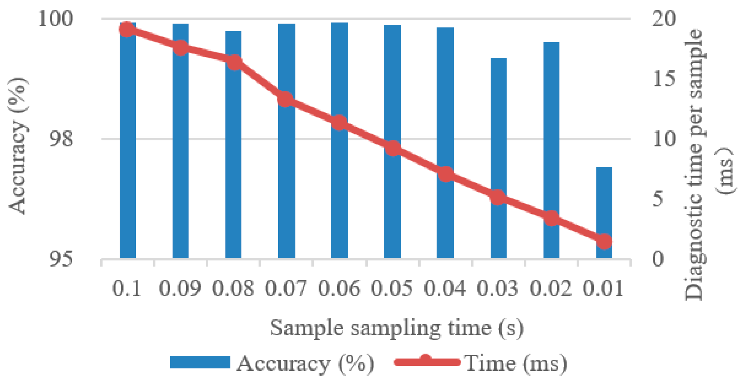
The data of 15 s for each operation condition is selected as a fault sample, and 0.1 s vibration signal is selected as a sample length. The dataset is divided into training, testing, and validation sets at a 5:2:3 ratio. The MD-CNN-BiLSTM method is used to train and test the dataset, and its accuracy is 99.94%. Because of the high sampling frequency of the vibration signal, the selection of the sample sampling duration affects the efficiency and accuracy of fault diagnosis. In order to test the effect of different sampling time frequencies of each sample on fault diagnosis, 10 kinds of sample lengths were selected according to the sampling time lengths of 0.01~0.1 s, with 0.01 s as the interval, which were trained and tested, respectively, and the results are shown in Figure 3. The proposed fault diagnosis model also achieves very good diagnostic results on the bearing natural-fault dataset, indicating that the proposed fault diagnosis model has good migration performance. When the sample sampling length is between 0.02 and 0.1 s, it has little effect on the model’s diagnostic performance, and accuracy remains above 99%. When the sample sampling length is lower than 0.02 s, the amount of information contained in each sample decreases as the amount of data decreases, and the network structure is relatively complex, which makes the model’s ability to extract fault characteristic information from a small amount of data decrease, resulting in poorer diagnostic results.

3.2. Generalisation Performance Test

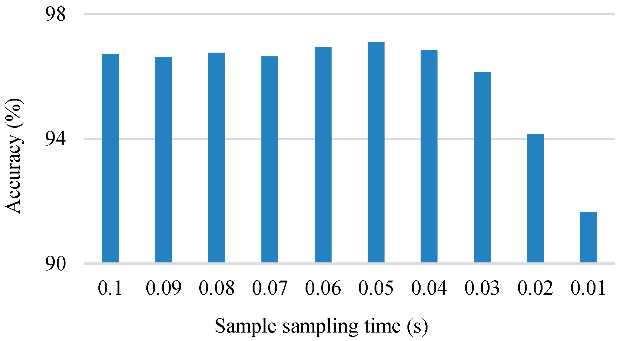
In order to test the generalisation ability of the model, the bearing data under three operation conditions were used for training, and then the data under another operation condition were used for testing. The test was conducted 10 times, and the average accuracy was calculated. The results are shown in Figure 4. The average diagnostic accuracy of the model under 10 sample sampling lengths is above 90%, with good generalisation ability. The diagnostic accuracy of the model increases with the increase in the sample length when the sample sampling length is between 0.01 and 0.06 s. When the sample sampling length is higher than 0.06 s, the average diagnostic accuracy, however, shows a decreasing trend.

3.3. Anti-Noise Test

From Figure 3 and Figure 4, it can be seen that the selection of the sample length affects the effectiveness of model fault diagnosis, and when the sample sampling length is 0.06 s, the model has better diagnostic accuracy and generalisation performance. In order to test the model’s ability to resist noise interference, the sample sampling length of 0.06 s is selected, and the Gaussian white noise signal with SNR of 10~80 dB and 10 dB intervals is added to the original vibration signals of the test set, respectively, and the bearing data under the three operation conditions (operation condition 1, 2, 3) are used for training and validation, and then the data under the other operation condition (operation condition 4) with the addition of different strengths of noise are used for testing, and the specific distribution of the dataset is shown in Table 4.
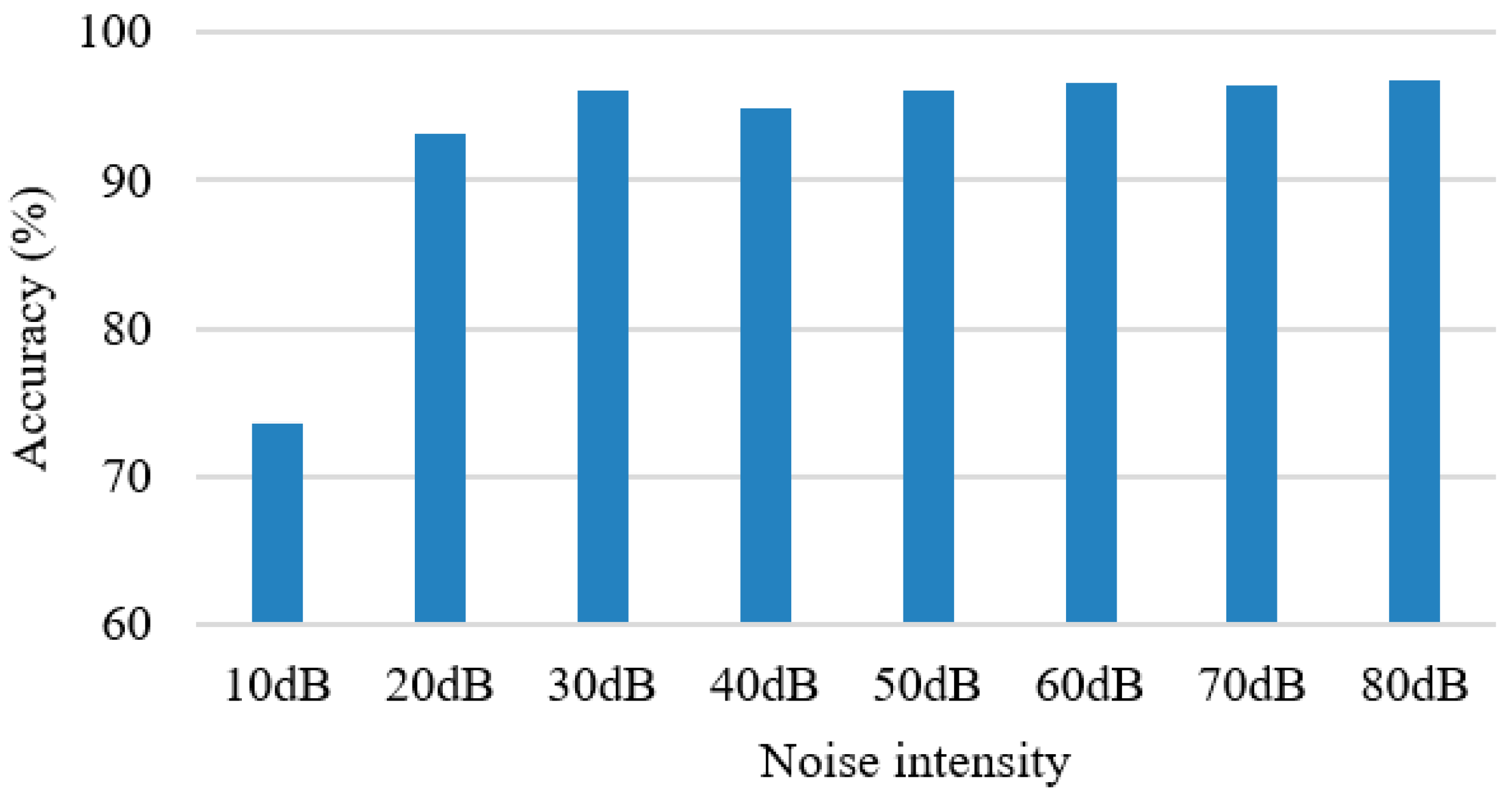
Each group of noise intensity test is also carried out 10 times, and the average accuracy is shown in Figure 5. The model can still maintain more than 90% diagnostic accuracy under noise interference between 20 and 80 dB, indicating that the model has both better noise resistance and generalisation ability. When the noise intensity is higher than 10 dB, the diagnostic accuracy and generalisation ability of the model decrease.

4. Data Imbalance Test for Traditional Class Weights

When the number of samples from different categories in a dataset varies greatly, the model may tend to favour the category with more data, resulting in insufficient learning of the category with fewer samples during training. Class weighting is one of the commonly used techniques when dealing with unbalanced datasets. By giving greater weight to fewer sample categories during training, the model pays more attention to a few categories of samples during training, thus balancing the influence of different categories and improving the model’s ability to learn from them. The class weights define the relative importance of each class for training, and the importance of different classes is balanced by adjusting the weights of the different classes in the loss function, which centres on assigning an appropriate weight value to each class, the value of which is usually proportional to the inverse of the number of samples in each class:
w i = N K n = 1 N t n i
where wi is the weight of the i-th category, K is the number of categories; N is the total number of samples; and tni is the n-th sample in the ith category.
Most deep learning-based fault diagnosis models are multi-classification networks, where the classification layer is usually located after the Softmax layer, and the cross-entropy function is used as the loss function. During network training, the classification layer computes cross-entropy loss by receiving values from the Softmax layer and assigns each input value to one of the K mutually independent categories using a 1-K coding scheme.
l o s s = 1 N n = 1 N i = 1 K w i t n i l n y n i
where is the probability that the nth sample output from the Softmax layer belongs to category i.
Various equipment of a ship is in normal operation most of the time, so the monitoring system can obtain a large amount of fault-free data, while the fault data is relatively very scarce. A high-performance condition monitoring system can accurately diagnose early equipment failures in a timely manner, so that repairs or replacements can be carried out even if they are needed to avoid further escalation of failures. However, due to conditions such as navigational conditions or mission requirements, the equipment needs to continue to operate with faults, which makes the faults more and more serious, and even leads to other component failures. Therefore, the amount and types of data for early failures are more than those for serious failures.

4.1. Test Analyses

Considering that the more serious and complex the faults of the equipment, the more difficult it is to obtain and the rarer the data, the training datasets with different percentage intervals are selected, and then a percentage number within the interval is randomly determined, and then samples with this percentage number are randomly selected from the dataset to simulate the data imbalance situation. All the data in the four states are used for training and testing, and the samples of the validation set and test set in each state are 200 and 300, respectively. The selection of the amount of unbalanced data in the training set is specified in Table 5.
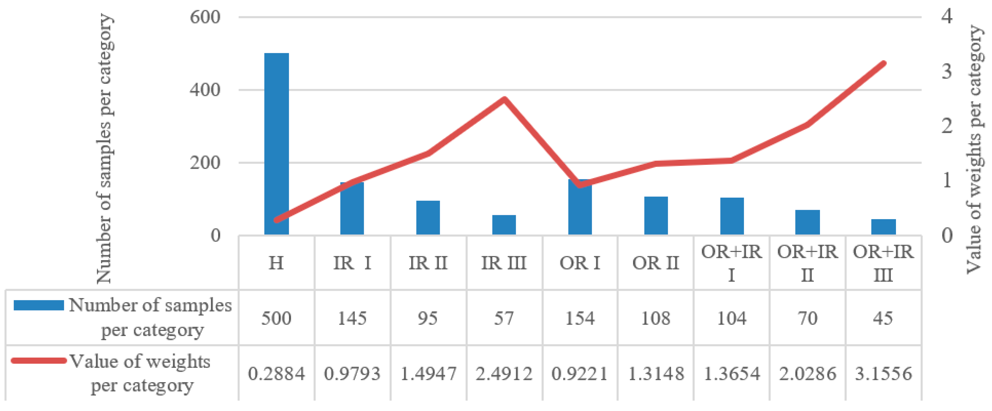
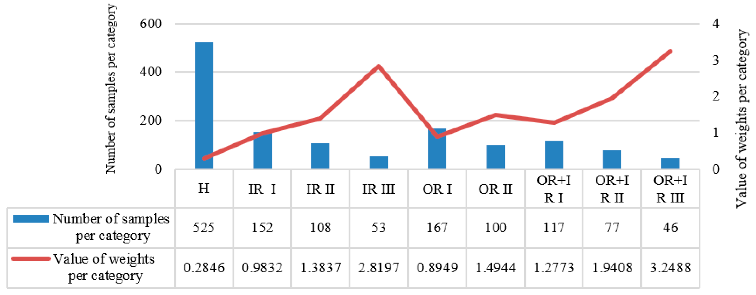
Figure 6 shows the number of data imbalance samples and their corresponding class weight values for each class in the training set; the fault severity is inversely proportional to the number of samples, which is consistent with the real fault data distribution. The class with fewer training samples has a larger corresponding weight value and can be more focused by the model during training.
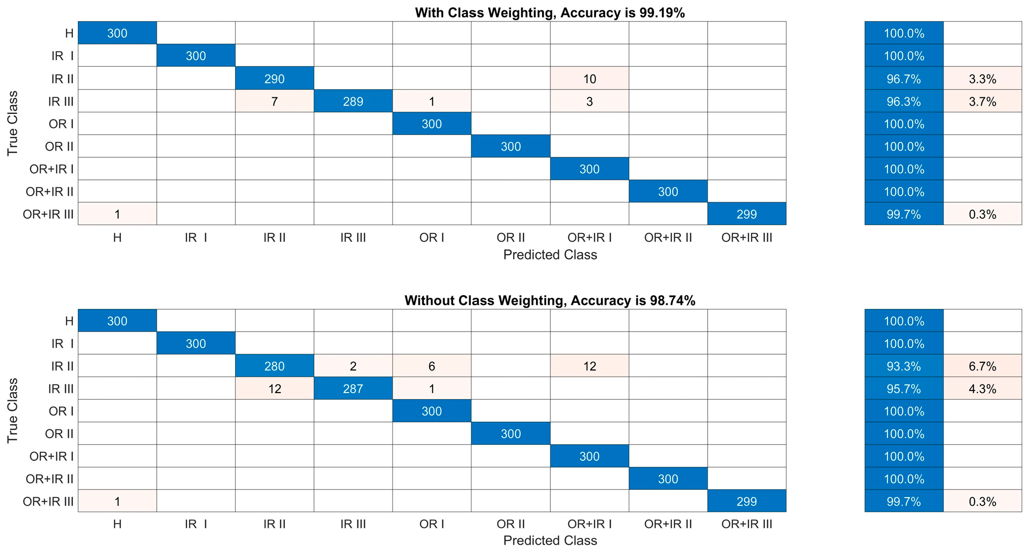
Figure 7 shows the diagnostic results of the model in both cases of adding class weights and no class weights, and the diagnostic accuracies of the model can maintain more than 98%, indicating that the model still has relatively high diagnostic accuracy even in the case of data imbalance when the training set contains all the operation condition data. In cases of data imbalance, adding class weights during training can improve learning for underrepresented classes, thereby enhancing the model’s fault diagnosis performance.
Precision and Recall are two other important metrics used to evaluate the performance of fault diagnosis models. Precision is concerned with the accuracy of the model in predicting positive categories and is defined as the ratio of the number of samples correctly predicted as faults by the model (True Positives, TP) to the number of all samples predicted as faults by the model (True Positives + False Positives, TP + FP), with the mathematical expression:
P r e c i s i o n = T P T P + F P
where TP is the number of faulty samples correctly predicted as faults by the model, and FP is the number of normal samples incorrectly predicted as faults by the model.
Recall measures the proportion of faulty samples correctly identified by the model to all actual faulty samples and reflects the ability to detect and identify faults. A higher recall rate means that the model is better able to capture fault samples, reduce missed diagnoses, and improve the comprehensiveness and reliability of fault diagnosis:
R e   c a l l = T P T P + F N
where False Negatives (FNs) is the number of faulty samples that the model predicts as normal.
In fault diagnosis, it is often desirable for the model to have high precision and recall. However, a high precision rate may be accompanied by a low recall rate (i.e., the model may miss some real faults). The F1 score, which is the reconciled average of the precision rate and the recall rate, is a metric that integrates the precision rate and the recall rate, avoids the limitations of a single metric, and enables a more comprehensive assessment of the model’s classification performance:
F 1 = 2 P r   e c i s i o n R e   c a l l P r   e c i s i o n + R e   c a l l
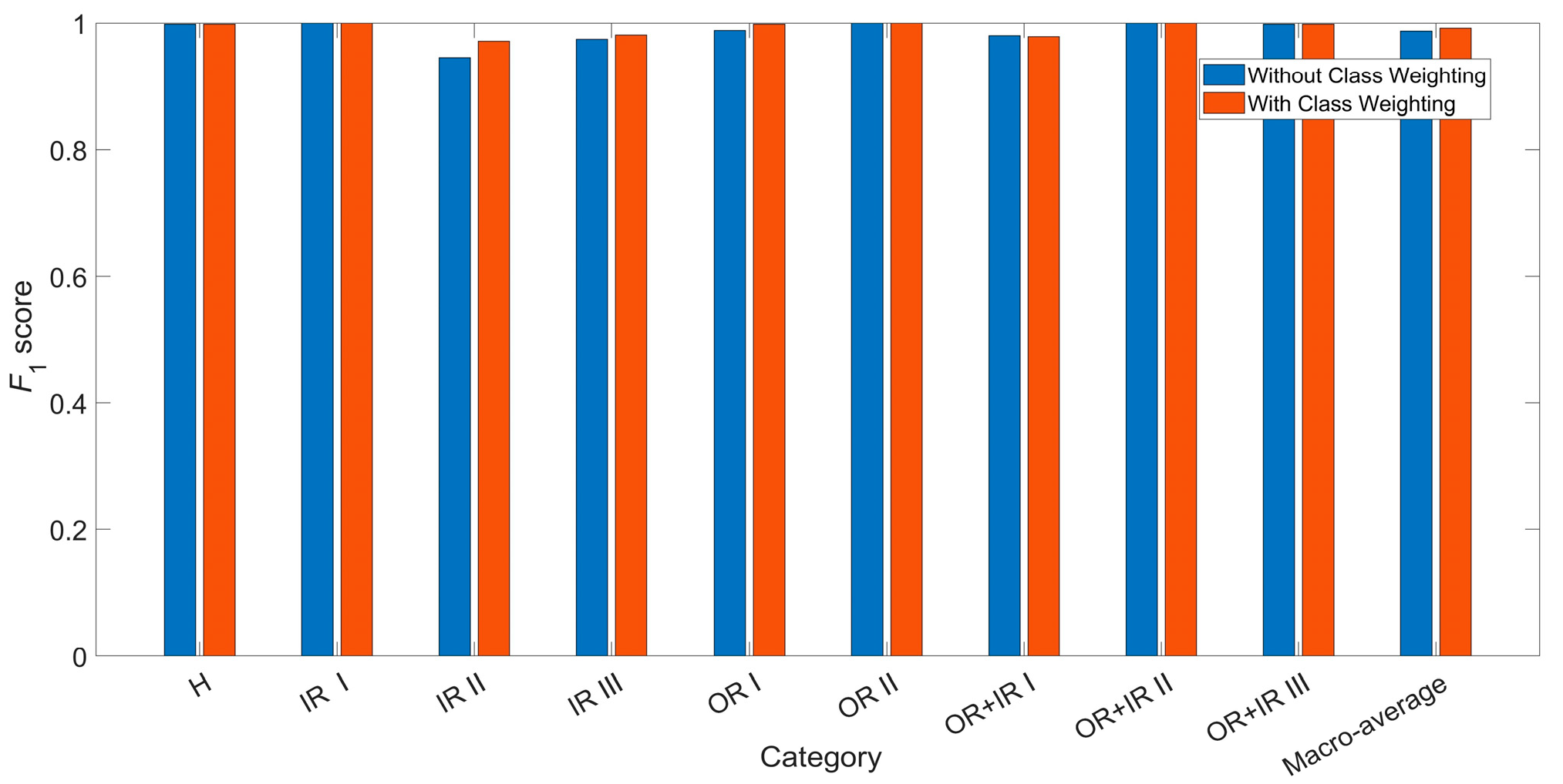
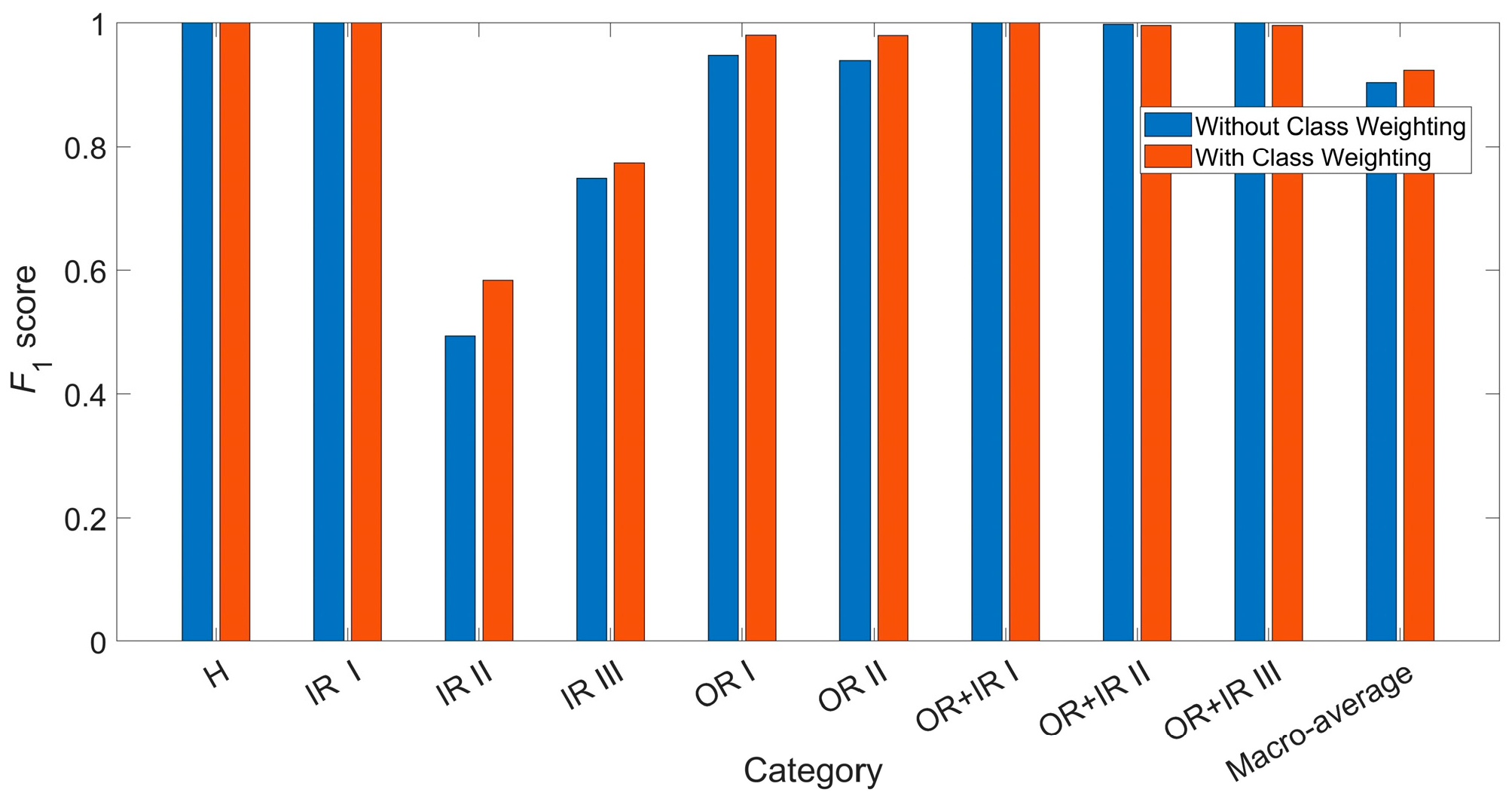
The F1 score ranges between 0 and 1, with values closer to 1 indicating better performance of the model. When both precision and recall are high, the F1 score will be closer to 1, indicating that the model performs better in terms of both precision and recall. Figure 8 shows the F1 scores for each category and the average obtained for both training methods of the model with the introduction of class weights and without class weights. Among the several states of the bearing, the lowest F1 score is obtained for the inner ring with class 2 failure, which has a small increase after the introduction of class weights. From the average F1 score, it can be seen that its value has increased to a certain extent after the introduction of class weights, which indicates that the introduction of class weights can improve the diagnostic effect of the model.

4.2. Generalisation Performance Test

Data from three states were used for training and validation, and data from another state was used for testing, so that the generalisation ability of the model could be tested. The samples of the validation and test sets for each state are 225 and 250, and the selection of the amount of unbalanced data in the training set is specified in Table 6.
Figure 9 shows the number of data imbalance samples and the corresponding weight values for each category of the training set, which still follows the principle that there are more normal samples than faulty samples, and more severe faulty samples than minor samples, which is in line with the distribution of real samples.
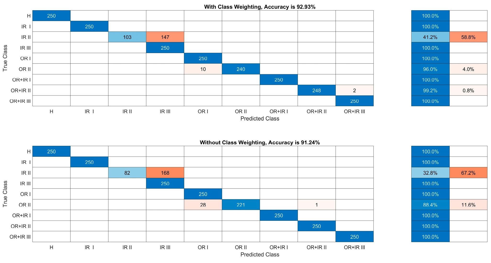
Figure 10 shows the diagnostic results of the model in both cases of adding class weights and no class weights. Before the introduction of class weights, the model was less effective in diagnosing class 2 faults in the outer ring and class 2 faults in the inner ring, with accuracy rates of 88.4% and 32.8%, respectively. After the introduction of class weights, the diagnostic effectiveness of these two classes of faults is significantly improved to 96.0% and 41.2%, which indicates that adding class weights during training can enhance the generalisation ability of the model and improve diagnostic accuracy. However, the diagnostic accuracy of inner-ring class 2 faults is very low regardless of whether class weights are added or not, and the model misdiagnoses inner-ring class 2 as inner-ring class 3 faults, because both faults are inner-ring faults with very similar vibration characteristics, but inner-ring class 2 faults have more samples, and the model is more sensitive to them, which may result in poorer performance on the category with more samples during testing.
Figure 11 shows the F1 scores for each category and the average obtained for both training methods of the model, introducing class weights and no class weights. It can be found that the F1 scores of the inner circle class 2, inner circle class 3 and outer circle class 1 faults are also affected by data balancing, with the inner circle class 2 having the lowest F1 score, indicating that this category is most affected by data imbalance and has the worst diagnostic effect. The introduction of class weights during the training process can improve the F1 scores to some extent, i.e., enhance the generalisation ability of the model, compared with the approach without class weights.

5. Data Imbalance Test for Dynamic Class Weights

5.1. Dynamic Class Weights

Too small weights may not be able to solve the class imbalance problem, while too large weights may cause the model to focus too much on a few classes, affecting generalisation performance for the majority. Traditional approaches to class weighting consider only the distribution of sample imbalances in each state of the device and do not take into account data characteristics and training situations. The fault characteristics between multiple states may be very similar; however, due to the effect of fixed class weights, it is easy for a certain class or some classes to have too much or too little weight during the training process, which affects the training effect of the model.
In order to solve the shortcomings of traditional fixed class weights, a dynamic class weighting method is proposed. The main idea of the method is to automatically and dynamically increase the weights of poorly trained classes during the training process so that they can receive more attention from the model and thus be fully learnt. The weight coefficient λ is introduced on the basis of the traditional class weights, which is used to correct the problem of too large or too small weights of certain classes in the training process. The weight coefficient λ consists of class weights w and F1 scores, and the F1 scores are usually used to comprehensively assess the diagnostic performance of the model, which can also reflect its training effect, and λ is expressed as follows:
λ i n = w i n F 1 i n
where λin is the weight coefficient of the n-th, i-th class, F1 in is the F1 score of the n-th, i-th class, and n is the number of updates of the dynamic class weights. When n is 1, it is the traditional class weight.
After each update, the new class weights are as follows:
w i n + 1 = w i n λ i n
By introducing the weight coefficient λ, it is able to adjust the class weight value according to the training situation. The weight coefficient λ enables increasing the weight of the poorly trained class in real time during the training process, and the worse the training effect, the larger its class weight becomes, ensuring the model learns better.

5.2. Test Analyses

All the data in the four bearing states are used for training and testing, and the validation set can reflect the current training effect and generalisation ability of the model, thus helping to adjust the model structure and parameters. The F1 scores of the validation set during the training process are used to adjust the dynamic weight coefficient λ. The validation set is validated every 2 iteration cycles during training, and the F1 scores of the validation set in the 10th, 20th, 30th, and 40th iteration cycles are selected to update the dynamic class weights, i.e., the new current class weights are calculated according to Equations (6) and (7). Table 7 shows changes in the class weights during the training process. Dynamic class weights can automatically adjust the class weight values according to the training effect during the training process to avoid the problem that some class weight values are too small. As the training proceeds, the class weights are constantly updated, and the F1 score of the validation set then gradually converges to 1, indicating that the training effect improves.
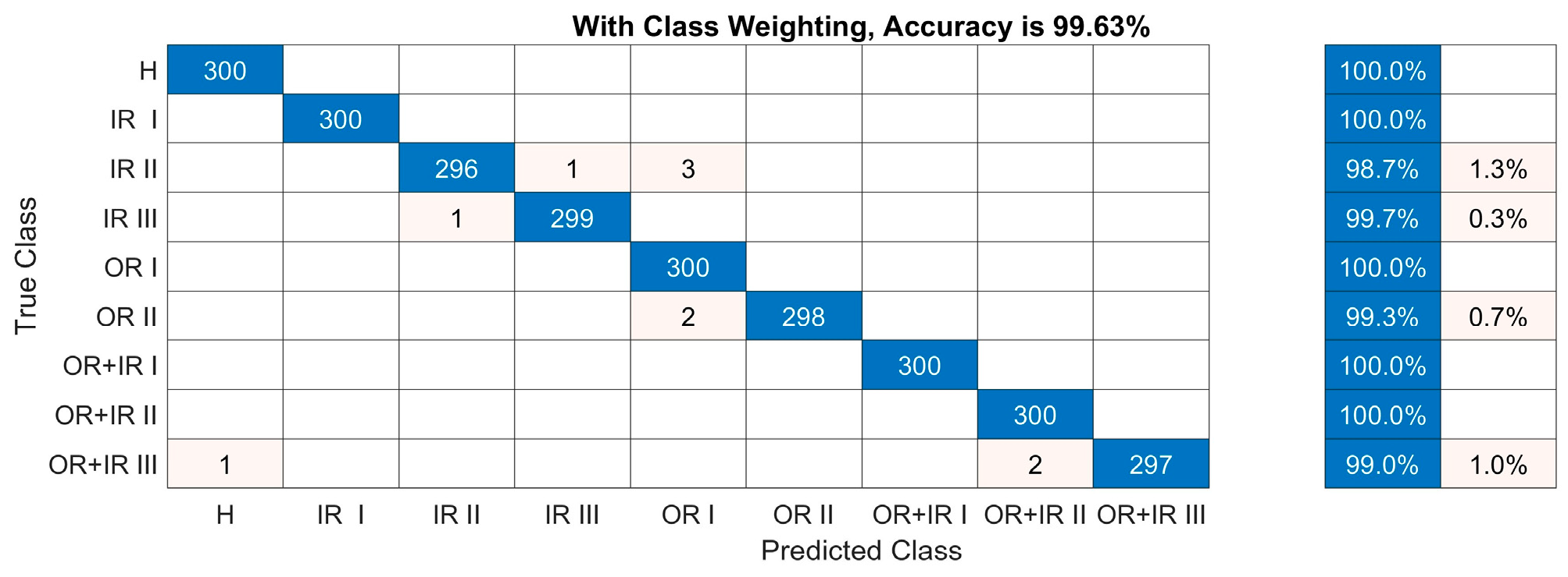
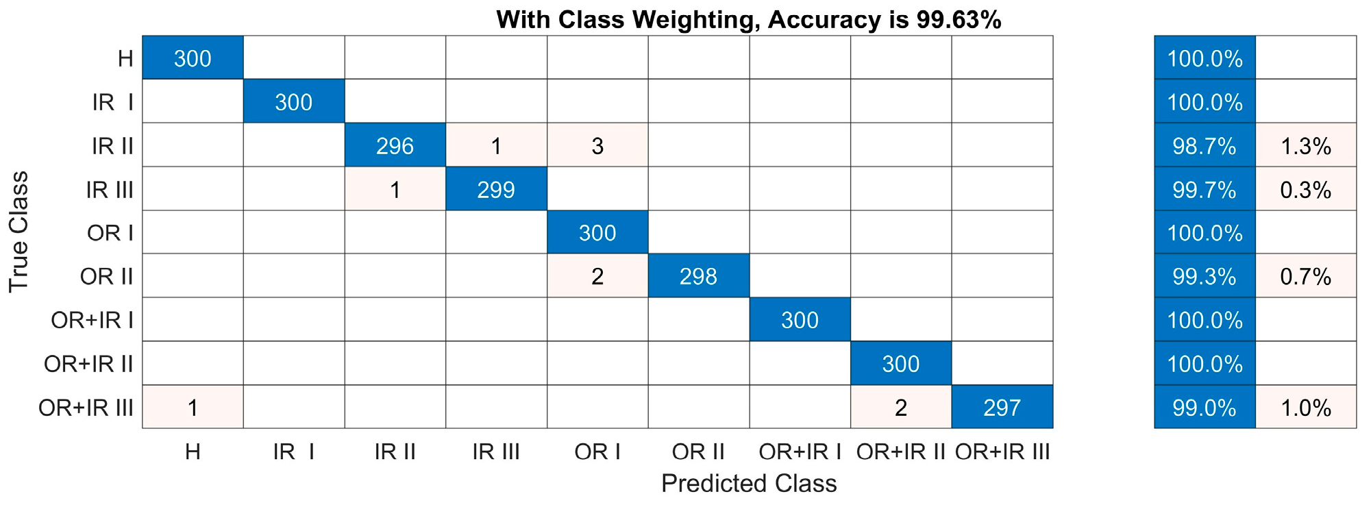
Figure 12 shows the diagnostic accuracy of the model introducing dynamic class weights, which reaches 99.63%, and provides very good diagnostic results. Compared with the diagnosis without class weights and traditional class weights, the proposed dynamic class weights method is more effective.
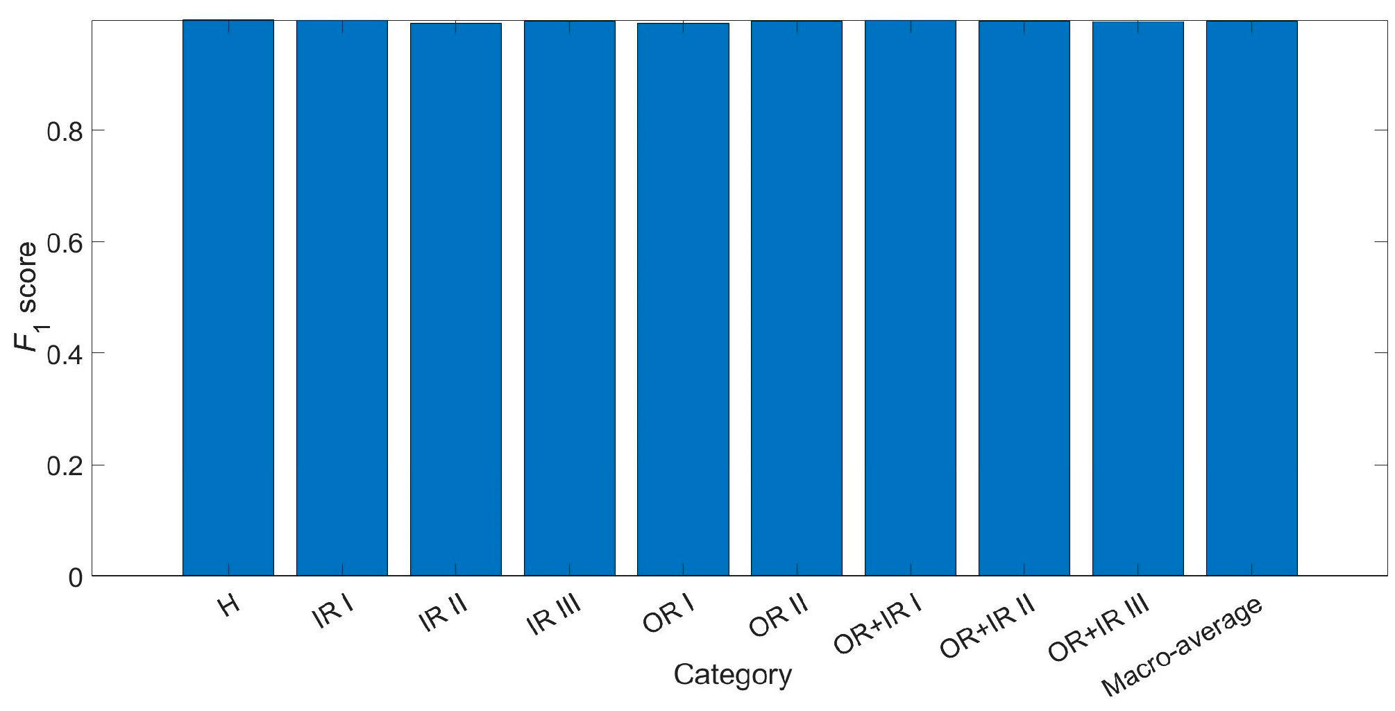
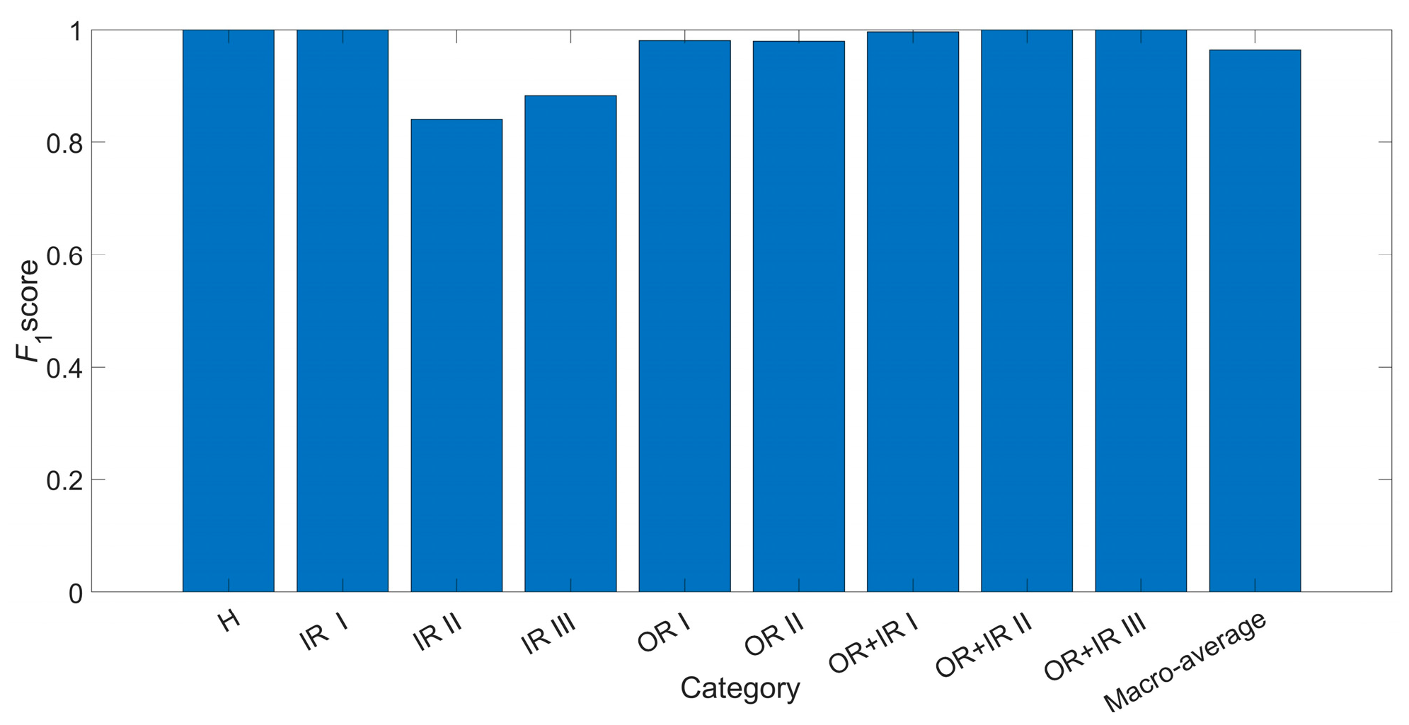
Figure 13 shows the F1 scores of the test set after the introduction of dynamic class weights to the model, and the F1 scores for each state of the bearing are very high, indicating that the trained model has both very good precision and recall and good overall performance.

5.3. Generalisation Test

Data from three states were used for training and validation, and then data from another state was used to test the generalisation ability of the model. The F1 scores of the validation set during training were also used to dynamically weight the coefficients λ. The class weights were updated at the 10th, 20th, 30th and 40th iteration cycles, and Table 8 shows the changes in the class weights during training. The dynamic class weights are continuously updated as the training proceeds, and the F1 scores for each class in the validation set gradually converge to 1, indicating that the accuracy and precision of the validation set are very high, and the training effect is better.
Figure 14 shows the diagnostic results of the model under brand-new operating conditions, and the diagnostic accuracy with the introduction of dynamic class weights reaches 96.49%, which has a very good generalisation ability. The inner circle class 2 fault is still the most misdiagnosed category; however, compared with the diagnostic results in Figure 6, Figure 7 and Figure 8 with no class weights and traditional class weights, the accuracy of this category has been greatly improved, with an accuracy of 72.4%, and the overall diagnostic accuracy has been increased by 3.56%.
Figure 15 shows the F1 scores for the test set after the introduction of dynamic class weights, and the inner circle class 2 and inner circle class 3 faults, although still two of the lower overall classes, show a very large improvement over the F1 scores of Figure 11 with no class weights and traditional class weights, suggesting that the dynamic class weights also improve the model’s performance by increasing both the precision and the recall of the model.

6. Conclusions

Class weighting is an effective measure to address data imbalance by adjusting the weight value of each class in the loss function to give more attention and importance to the classes with fewer data samples, thus balancing the importance of different classes. The traditional class weighting method calculates class weights based on the number of samples in each category; however, it ignores the influence of data characteristics and the training process. To address this issue, a dynamic class weighting method is proposed that enables traditional class weighting methods to adjust weight values.
A class weight coefficient λ is introduced on the basis of traditional class weights, which is obtained from the F1 scores of the validation set during the training process, because the validation set reflects the training effect of the model, and the F1 scores comprehensively assess the classification results of the validation set. The class weight coefficient λ is used to update the class weight value according to the validation set results of a specific iteration cycle during the training process so that poorly trained classes receive a larger weight and gain more attention from the model and thus are adequately learnt. The experimental results show that the method of dynamic class weighting can effectively improve the training effect of the model, and the diagnostic results under brand-new operation conditions show that the accuracy rate is 5.25% higher than that of no class weighting and 3.56% higher than that of the traditional class weighting method, which makes the model have better generalisation performance.

Author Contributions

Methodology, G.Y. and J.K.; Software, G.Y.; Validation, J.K.; Formal analysis, X.W. and K.L.; Writing—original draft, G.Y.; Writing—review & editing, X.W. and K.L.; Visualization, X.W.; Supervision, X.Y.; Project administration, X.Y.; Funding acquisition, X.Y. All authors have read and agreed to the published version of the manuscript.

Funding

This research was funded by [Ningbo Key R&D Programme Project] grant number [2023Z036].

Data Availability Statement

The data presented in this study are openly available in [Data Sets and Download] at [https://mb.uni-paderborn.de/kat/forschung/kat-datacenter/bearing-datacenter/data-sets-and-download].

Conflicts of Interest

Author Jingran Kang was employed by the company Geely Automobile Research Institute (Ningbo) Co., Ltd. The remaining authors declare that the research was conducted in the absence of any commercial or financial relationships that could be construed as a potential conflict of interest.

References

  1. Orlowska-Kowalska, T.; Wolkiewicz, M.; Pietrzak, P.; Skowron, M.; Ewert, P.; Tarchala, G.; Krzysztofiak, M.; Kowalski, C.T. Fault Diagnosis and Fault-Tolerant Control of PMSM Drives–State of the Art and Future Challenges. IEEE Access 2022, 10, 59979–60024. [Google Scholar] [CrossRef]
  2. Zhang, S.; Zhang, S.; Wang, B.; Habetler, T.G. Deep Learning Algorithms for Bearing Fault Diagnostics—A Comprehensive Review. IEEE Access 2020, 8, 29857–29881. [Google Scholar] [CrossRef]
  3. Zhao, Z.; Xu, Q.; Jia, M. Improved shuffled frog leaping algorithm-based BP neural network and its application in bearing early fault diagnosis. Neural Comput. Appl. 2016, 27, 375–385. [Google Scholar] [CrossRef]
  4. Mohammad-Alikhani, A.; Nahid-Mobarakeh, B.; Hsieh, M.F. One-Dimensional LSTM-Regulated Deep Residual Network for Data-Driven Fault Detection in Electric Machines. IEEE Trans. Ind. Electron. 2024, 71, 3083–3092. [Google Scholar] [CrossRef]
  5. Verstraete, D.; Ferrada, A.; Droguett, E.L.; Meruane, V.; Modarres, M. Deep Learning Enabled Fault Diagnosis Using Time-Frequency Image Analysis of Rolling Element Bearings. Shoc. Vib. 2017, 2017, 5067651. [Google Scholar] [CrossRef]
  6. Ayas, S.; Ayas, M.S. A novel bearing fault diagnosis method using deep residual learning network. Multimed. Tools Appl. 2022, 81, 22407–22423. [Google Scholar] [CrossRef]
  7. Deveci, B.U.; Celtikoglu, M.; Albayrak, O.; Unal, P.; Kirci, P. Transfer Learning Enabled Bearing Fault Detection Methods Based on Image Representations of Single-Dimensional Signals. Inf. Syst. Front. 2024, 26, 1345–1397. [Google Scholar] [CrossRef]
  8. Khan, M.A.; Kim, Y.-H.; Choo, J. Intelligent fault detection using raw vibration signals via dilated convolutional neural networks. J. Supercomput. 2020, 76, 8086–8100. [Google Scholar] [CrossRef]
  9. Guo, Y.; Mao, J.; Zhao, M. Rolling Bearing Fault Diagnosis Method Based on Attention CNN and BiLSTM Network. Neural Process. Lett. 2023, 55, 3377–3410. [Google Scholar] [CrossRef]
  10. Wang, Y.; Cao, G. A multiscale convolution neural network for bearing fault diagnosis based on frequency division denoising under complex noise conditions. Complex Intell. Syst. 2023, 9, 4263–4285. [Google Scholar] [CrossRef]
  11. Van Horn, G.; Mac Aodha, O.; Song, Y.; Cui, Y.; Sun, C.; Shepard, A.; Adam, H.; Perona, P.; Belongie, S. The inaturalist species classification and detection dataset. In Proceedings of the IEEE Conference on Computer Vision and Pattern Recognition, Salt Lake City, UT, USA, 18–23 June 2018; pp. 8769–8778. [Google Scholar]
  12. Gupta, A.; Dollar, P.; Girshick, R. Lvis: A dataset for large vocabulary instance segmentation. In Proceedings of the IEEE/CVF Conference on Computer Vision and Pattern Recognition, Long Beach, CA, USA, 15–20 June 2019; pp. 5356–5364. [Google Scholar]
  13. Bansal, M.A.; Sharma, D.R.; Kathuria, D.M. A systematic review on data scarcity problem in deep learning: Solution and applications. ACM Comput. Surv. (CSUR) 2022, 54, 208. [Google Scholar] [CrossRef]
  14. Mahajan, D.; Girshick, R.; Ramanathan, V.; He, K.; Paluri, M.; Li, Y.; Bharambe, A.; Van Der Maaten, L. Exploring the limits of weakly supervised pretraining. In Proceedings of the European Conference on Computer Vision (ECCV), Munich, Germany, 8–14 September 2018; pp. 181–196. [Google Scholar]
  15. Mikolov, T.; Sutskever, I.; Chen, K.; Corrado, G.S.; Dean, J. Distributed representations of words and phrases and their compositionality. In Proceedings of the Advances in Neural Information Processing Systems 26, Lake Tahoe, NV, USA, 5–10 December 2013. [Google Scholar]
  16. Fan, B.; Ma, H.; Liu, Y.; Yuan, X. BWLM: A Balanced Weight Learning Mechanism for Long-Tailed Image Recognition. Appl. Sci. 2024, 14, 454. [Google Scholar] [CrossRef]
  17. Lessmeier, C.; Kimotho, J.K.; Zimmer, D.; Sextro, W. Condition monitoring of bearing damage in electromechanical drive systems by using motor current signals of electric motors: A benchmark data set for data-driven classification. In Proceedings of the PHM Society European Conference, Bilbao, Spain, 5–8 July 2016; Volume 3. [Google Scholar]
  18. Zhang, W.; Li, X.; Ding, Q. Deep residual learning-based fault diagnosis method for rotating machinery. ISA Trans. 2019, 95, 295–305. [Google Scholar] [CrossRef] [PubMed]
  19. Huang, R.; Liao, Y.; Zhang, S.; Li, W. Deep Decoupling Convolutional Neural Network for Intelligent Compound Fault Diagnosis. IEEE Access 2019, 7, 1848–1858. [Google Scholar] [CrossRef]
  20. Ding, X.; He, Q. Energy-Fluctuated Multiscale Feature Learning with Deep ConvNet for Intelligent Spindle Bearing Fault Diagnosis. IEEE Trans. Instrum. Meas. 2017, 66, 1926–1935. [Google Scholar] [CrossRef]
  21. Yuan, J.; Yao, Z.; Zhao, Q.; Xu, Y.; Li, C.; Jiang, H. Dual-Core Denoised Synchrosqueezing Wavelet Transform for Gear Fault Detection. IEEE Trans. Instrum. Meas. 2021, 70, 3521611. [Google Scholar] [CrossRef]
  22. Smith, W.A.; Randall, R.B. Rolling element bearing diagnostics using the Case Western Reserve University data: A benchmark study. Mech. Syst. Signal Process. 2015, 64–65, 100–131. [Google Scholar] [CrossRef]
  23. Zhao, Z.; Jiao, Y.; Zhang, X. A Fault Diagnosis Method of Rotor System Based on Parallel Convolutional Neural Network Architecture with Attention Mechanism. J. Signal Process. Syst. 2023, 95, 965–977. [Google Scholar] [CrossRef]
  24. Yan, G.; Hu, Y. Inter-turn short circuit and demagnetization fault diagnosis of ship PMSM based on multiscale residual dilated CNN and BiLSTM. Meas. Sci. Technol. 2024, 35, 046105. [Google Scholar] [CrossRef]
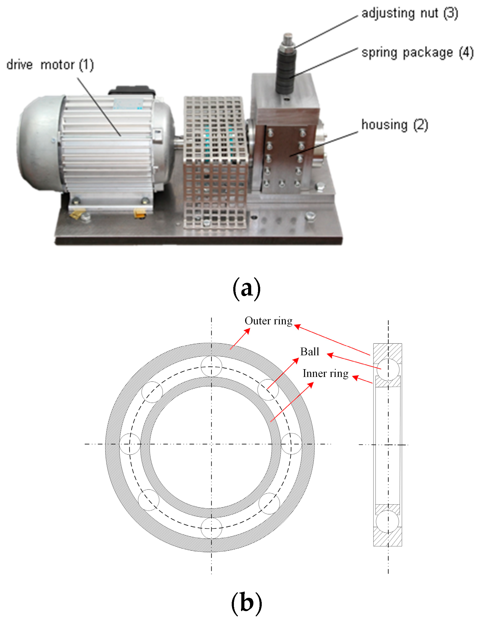
Figure 1. Apparatus for accelerated life time test. (a) Bearing accelerated life test rig [17]. (b) Schematic diagram of grooved ball bearings.
Jmse 13 02204 g001
Figure 2. Bearing test rig [17].
Jmse 13 02204 g002
Figure 3. Model at different sampling times, diagnostic accuracy and diagnostic time consumption.
Jmse 13 02204 g003
Figure 4. Generalisation performance of the model with different sampling times.
Jmse 13 02204 g004
Figure 5. Generalisation ability of the model in the presence of noise.
Jmse 13 02204 g005
Figure 6. The number of samples in each category of the training set and the corresponding class weight values.
Jmse 13 02204 g006
Figure 7. Diagnostic accuracy in two scenarios.
Jmse 13 02204 g007
Figure 8. F1 scores for each state and the average of the bearings.
Jmse 13 02204 g008
Figure 9. The number of samples in each category of the training set and the corresponding class weight values.
Jmse 13 02204 g009
Figure 10. Diagnostic accuracy in two scenarios.
Jmse 13 02204 g010
Figure 11. F1 scores for each state and the average of the bearings.
Jmse 13 02204 g011
Figure 12. Diagnostic accuracy with the introduction of dynamic class weights.
Jmse 13 02204 g012
Figure 13. Test set F1 scores after introducing dynamic class weights.
Jmse 13 02204 g013
Figure 14. Diagnostic accuracy with the introduction of dynamic class weights.
Jmse 13 02204 g014
Figure 15. Test set F1 scores after introducing dynamic class weights.
Jmse 13 02204 g015
Table 1. Bearing Fault Levels [17].
Damage LevelPercentage of Damage Length to Pitch CircumferenceCorresponding Damage Range of Test Bearing
10~2%≤2 mm
22~5%>2 mm
35~15%>4.5 mm
415~35%>13.5 mm
5>35%>31.5 mm
Table 2. Test conditions [17].
Test Operation ConditionSpeed (r/min)Load Torque (Nm)Radial Force (N)
115000.71000
29000.71000
315000.11000
415000.7400
Table 3. Bearing test details [17].
StatusDamage LevelCode
Health H
Inner ring damage1IR I
2IR II
3IR III
Outer ring damage1OR I
2OR II
Damage to both inner and outer rings1IR + OR I
2IR + OR II
3IR + OR III
Table 4. Bearing fault types and the number of samples.
Fault TypeTraining SamplesValidation SamplesTest SampleStatus Code
Health525225250H
Inner ring level 1525225250IR I
Inner ring level 2525225250IR II
Inner ring level 3525225250IR III
Outer ring level 1525225250OR I
Outer ring level 2525225250OR II
Compound fault level 1525225250IR + OR I
Compound fault level 2525225250IR + OR II
Compound fault level 3525225250IR + OR III
Table 5. Training set sample imbalance settings.
Fault TypeTraining SamplesPercentage Range (%)Unbalanced Sample IntervalsStatus Code
Health500100500H
Inner ring level 150020~30100~150IR I
Inner ring level 250010~2050~100IR II
Inner ring level 35005~1025~50IR III
Outer ring level 150020~30100~150OR I
Outer ring level 250010~2050~100OR II
Compound fault level 150015~2075~100IR + OR I
Compound fault level 250010~1550~75IR + OR II
Compound fault level 35005~1025~50IR + OR III
Table 6. Training set sample imbalance settings.
Fault TypeTraining SamplesPercentage Range (%)Unbalanced Sample IntervalsStatus Code
Health525100525H
Inner ring level 152520~30105~158IR I
Inner ring level 252510~2053~105IR II
Inner ring level 35255~1026~53IR III
Outer ring level 152520~30105~158OR I
Outer ring level 252510~2053~105OR II
Compound fault level 152515~2079~105IR + OR I
Compound fault level 252510~1553~79IR + OR II
Compound fault level 35255~1026~53IR + OR III
Table 7. Dynamic class weight changes during model training and F1 scores for the validation set.
Iteration PeriodItemsHealthInner Ring Level 1Inner Ring Level 2Inner Ring Level 3Outer Ring Level 1Outer Ring Level
2
Compound Fault Level 1Compound Fault Level 2Compound Fault Level 3
1Number of class samples5001639744149971047456
Initial class weights0.290.951.442.800.941.321.371.972.47
10F1 scores1.001.000.720.760.970.990.951.001.00
Updated category weights0.290.951.923.250.981.361.421.972.48
20F1 scores1.000.990.830.740.990.980.930.990.99
Updated category weights0.290.962.343.850.981.381.511.982.47
30F1 scores1.001.000.950.880.991.000.991.001.00
Updated category weights0.290.962.714.661.011.381.531.982.47
40F1 scores1.001.000.991.001.001.001.001.001.00
Updated category weights0.290.962.734.681.021.391.531.982.48
Table 8. Dynamic class weight changes during model training and F1 scores for the validation set.
Iteration PeriodItemsHealthInner Ring Level 1Inner Ring Level 2Inner Ring Level 3Outer Ring Level 1Outer Ring Level
2
Compound Fault Level 1Compound Fault Level 2Compound Fault Level 3
1Number of class samples525146110451661111177452
Initial class weights0.291.021.353.320.901.351.282.022.88
10F1 scores0.991.000.680.870.920.980.901.001.00
Updated category weights0.291.031.993.820.971.371.422.022.89
20F1 scores1.001.000.990.980.920.941.001.001.00
Updated category weights0.291.031.993.871.061.461.422.022.89
30F1 scores1.001.000.990.991.001.001.001.001.00
Updated category weights0.291.032.013.891.061.461.422.022.90
40F1 scores1.001.000.991.001.001.000.991.001.00
Updated category weights0.291.032.033.901.061.461.442.022.91
Disclaimer/Publisher’s Note: The statements, opinions and data contained in all publications are solely those of the individual author(s) and contributor(s) and not of MDPI and/or the editor(s). MDPI and/or the editor(s) disclaim responsibility for any injury to people or property resulting from any ideas, methods, instructions or products referred to in the content.